Sneutrino Inflation

SNEUTRINO INFLATION

Abstract

The seesaw model of neutrinos might explain the size, age, flatness and near-homogeneity of the Universe via sneutrino inflation, as well as explaining the origin of matter via leptogenesis. The sneutrino inflation hypothesis makes specific, testable predictions for cosmic microwave background observables, which are compatible with the first release of data from WMAP, and for flavour-violating charged-lepton decays. In particular, $\mu\to e\gamma$ should occur with a branching ratio very close to the present experimental upper limit, whilst $\tau\to\mu\gamma$ and $e\gamma$ should occur further below the present limits.

Invited talk at the Fujihara Seminar on Neutrino Mass and Seesaw Mechanism, KEK, Feb. 23-25, 2004

1 INTRODUCTION

What is the connection between the data on the cosmic microwave background (CMB) from WMAP [1] and searches for $\mu\to e\gamma$ and other charged-lepton flavour-violating (LFV) processes? One may be provided by sneutrino inflation, an idea first proposed by Murayama-san, Suzuki-san, Yanagida-san and Yokoyama-san [2, 3]. This appealing idea languished in obscurity for over a decade, for reasons that are unknown to me. Personally, although I have always been attracted towards inflationary cosmology, I have been reluctant to embrace it wholeheartedly, largely because of the absence of a convincing candidate for the inflaton field. Only recently did it dawn upon me that the supersymmetric spin-zero partner of one of the heavy singlet neutrinos in the seesaw might be a suitable candidate. My interest was then stimulated by the first release of data from the WMAP satellite [1], which were consistent with many key inflationary predictions, such as the Gaussian nature and almost scale invariance of the primordial density perturbations. Moreover, the WMAP data excluded many rival inflationary models, such as those with a simple quartic potential, for example.

Last year, Raidal, Yanagida-san and I [4] revived the sneutrino inflation idea, calculated several inflationary observables such as the scalar spectral index (tilt) and the magnitude of the tensor perturbations relative to the scalar modes, showed they were consistent with the WMAP data, used the model to constrain the seesaw parameters, and finally calculated LFV processes showing, for example, that $\mu\to e\gamma$ might occur not far below the present experimental limit. More recently, Chankowski, Pokorski, Raidal, Turzynski and I [5] have explored in more detail the sneutrino inflation predictions for LFV processes. This talk is based on these two papers.

First, however, I summarize the basic features of inflation [6]. Then I recall the 18 parameters of the minimal three-generation seesaw model [7], and how they appear in low-energy LFV observables as well as neutrino oscillations and leptogenesis [8, 9]. Then I compare the predictions of sneutrino inflation [4] with WMAP data [1] and recall that the gravitino problem [10] favours non-thermal scenarios for leptogenesis [4]. Finally, I dissect [5] the predictions of sneutrino inflation for various LFV processes [4], showing how they follow from the (near) decoupling of the sneutrino inflaton, which is motivated by the gravitino problem and some approaches to neutrino masses within the seesaw model [11].

2 SUMMARY OF INFLATIONARY COSMOLOGY

The basic idea of cosmological inflation [12] is that, at some early epoch in the history of the Universe, its energy density may have been dominated by an almost constant term:

$$\left({{\dot{a}}\over a}\right)^{2}\;=\;{8\pi G_{N}\rho\over 3}-{k\over a^{2}}:\;\;\rho\;=\;V,$$ (1)

leading to a phase of near-exponential de Sitter expansion. It is easy to see that the second (curvature) term in (1) rapidly becomes negligible, and that

$$a\;\simeq\;a_{I}e^{Ht}:\;\;H\;=\;\sqrt{{8\pi G_{N}\over 3}V}$$ (2)

during this inflationary expansion, if $V$ is really constant.

In this case, the horizon would also have expanded (near-) exponentially, so that the entire visible Universe might have been within our pre-inflationary horizon:

$$a_{H}\;\simeq\;a_{I}e^{H\tau}\;\gg\;c\tau,$$ (3)

where $H\tau$ is the number of e-foldings during inflation. This would have enabled our observable universe to appear (almost) homogeneous. Since the $-{k\over a^{2}}$ term in (1) becomes negligible, the Universe may now appear almost flat with $\Omega_{tot}\simeq 1$. However, as we see later, perturbations during inflation generate a small deviation from unity: $|\Omega_{tot}-1|\simeq 10^{-5}$. Following inflation, the conversion of the inflationary vacuum energy into particles reheats the Universe, filling it with the required entropy. Finally, the closest pre-inflationary monopole or gravitino is pushed away, further than the origin of the CMB, by the exponential expansion of the Universe.

The above description is quite classical. In fact, one should expect quantum fluctuations in the initial value of the inflaton field $\phi$, which would cause the inflationary expansion to be slightly inhomogeneous [6], with different parts of the Universe expanding at slightly different rates. These quantum fluctuations would give rise to a Gaussian random field of density perturbations with similar magnitudes on different scale sizes, just as the astrophysicists have long wanted [13]. The magnitudes of these perturbations would be linked to the value of the effective potential during inflation, and would be visible in the CMB as adiabatic temperature fluctuations [6]:

$${\delta T\over T}\;\sim\;{\delta\rho\over\rho}\;\sim\;\mu^{2}G_{N},$$ (4)

where $\mu\equiv V^{1/4}$ is a typical vacuum energy scale during inflation. Consistency with the cosmic microwave background (CMB) data from COBE et al., that find $\delta T/T\simeq 10^{-5}$, is obtained if

$$\mu\;\simeq\;10^{16}~{}{\rm GeV},$$ (5)

comparable with the GUT scale.

One example of such a scenario is chaotic inflation [14], according to which there is no special structure in the effective potential $V(\phi)$, which might be a simple power $V\sim\phi^{n}$ or exponential $V\sim e^{\alpha\phi}$. In this scenario, any given region of the Universe is assumed to start with some random value of the inflaton field $\phi$ and hence the potential $V(\phi)$, which decreases monotonically to zero. The equation of motion of the inflaton field is

$${\ddot{\phi}}\;+\;3H{\dot{\phi}}\;+\;V^{\prime}(\phi)\;=\;0,$$ (6)

and (our part of) the Universe undergoes sufficient expansion if the initial value of $V(\phi)$ is large enough, and the potential flat enough. The first term in (6) is assumed to be negligible, in which case the equation of motion is dominated by the second (Hubble drag) term, and one has

$${\dot{\phi}}\;\simeq\;-{V^{\prime}\over 3H}.$$ (7)

In this slow-roll approximation, $\phi$ rolls slowly down the potential if

$$\epsilon\; \equiv \;{1\over 2}M_{P}^{2}\left({V^{\prime}\over V}\right)^{2},\;\eta\;\equiv M_{P}^{2}\left({V^{\prime\prime}\over V}\right)~{},$$ (8)

$$\xi\; \equiv \;M_{P}^{4}\left({VV^{\prime\prime\prime}\over V^{2}}\right)$$

are all $\ll 1$, where $M_{P}\equiv 1/\sqrt{8\pi G_{N}}\simeq 2.4\times 10^{18}$ GeV. Various observable quantities can then be expressed in terms of $\epsilon,\eta$ and $\xi$ [6], including the spectral index for scalar density perturbations:

$$n_{s}\;=\;1\;-\;6\epsilon\;+\;2\eta,$$ (9)

the ratio of scalar and tensor perturbations at the quadrupole scale:

$$r\;\equiv{A_{T}\over A_{S}}=16\epsilon,$$ (10)

the spectral index of the tensor perturbations:

$$n_{T}\;=\;-2\epsilon,$$ (11)

and the running parameter for the scalar spectral index:

$${dn_{s}\over d{\rm ln}k}\;=\;{2\over 3}\left[\left(n_{s}-1\right)^{2}-4\eta^{2}\right]+2\xi.$$ (12)

The amount $e^{N}$ by which the Universe expanded during inflation is also controlled [6] by the slow-roll parameter $\epsilon$:

$$e^{N}:\;N\;=\;\int Hdt\;=\;{2\sqrt{\pi}\over m_{P}}\int^{\phi_{final}}_{\phi_{initial}}{d\phi\over\sqrt{\epsilon(\phi)}}.$$ (13)

In order to explain the size of a feature in the observed Universe, one needs:

$$N\; = \;62-{\rm ln}{k\over a_{0}H_{0}}-{\rm ln}{10^{16}{\rm GeV}\over V_{k}^{1/4}}+{1\over 4}{\rm ln}{V_{k}\over V_{e}}$$ (14)

$$- {1\over 3}{\rm ln}{V_{e}^{1/4}\over\rho_{RH}^{1/4}}\sim 50\;{\rm to}\;70,$$

where $k$ characterizes the size of the feature, $V_{k}$ is the magnitude of the inflaton potential when the feature left the horizon, $V_{e}$ is the magnitude of the inflaton potential at the end of inflation, and $\rho_{RH}$ is the density of the Universe immediately following reheating after inflation.

As an example of the above general slow-roll theory, let us consider chaotic inflation [14] with a $V={1\over 2}m^{2}\phi^{2}$ potential, as appears in the sneutrino inflation model [4] discussed later. In this model, the conventional slow-roll inflationary parameters are

$$\epsilon\;=\;{2M_{P}^{2}\over\phi_{I}^{2}},\;\eta\;=\;{2M_{P}^{2}\over\phi_{I}^{2}},\;\xi\;=\;0,$$ (15)

where $\phi_{I}$ denotes the a priori unknown inflaton field value during inflation at a typical CMB scale $k$. The overall scale of the inflationary potential is normalized by the WMAP data on density fluctuations:

$$\Delta_{R}^{2} = {V\over 24\pi^{2}M_{P}^{2}\epsilon}=2.95\times 10^{-9}A~{},$$ (16)

$$A = 0.77\pm 0.07,$$

yielding

$$V^{1\over 4} = M_{P}^{4}\sqrt{\epsilon\times 24\pi^{2}\times 2.27\times 10^{-9}}$$

$$= 0.027M_{P}\times\epsilon^{1\over 4},$$

corresponding to

$$m^{1\over 2}\phi_{I}\;=\;0.038\times M_{P}^{3\over 2}$$ (18)

in any simple chaotic $\phi^{2}$ inflationary model. The above expression (14) for the number of e-foldings after the generation of the CMB density fluctuations observed by COBE could be as low as $N\simeq 50$ for a reheating temperature $T_{RH}$ as low as $10^{6}$ GeV. In the $\phi^{2}$ inflationary model, this value of $N$ would imply

$$N\;={1\over 4}{\phi^{2}_{I}\over M_{P}^{2}}\simeq\;50,$$ (19)

corresponding to

$$\phi^{2}_{I}\simeq 200\times M_{P}^{2}.$$ (20)

Inserting this requirement into the WMAP normalization condition (2), we find [4] the following required mass for any inflaton with a simple quadratic potential:

$$m\;\simeq 2\times 10^{13}~{}{\rm GeV}.$$ (21)

This is comfortably within the range of heavy singlet (s)neutrino masses usually considered, namely $m_{N}\sim 10^{10}$ to $10^{15}$ GeV, motivating the sneutrino inflation model discussed below.

Is this simple $\phi^{2}$ model compatible with the WMAP data? It predicts the following values for the primary CMB observables [4]: the scalar spectral index

$$n_{s}\;=\;1-{8M_{P}^{2}\over\phi^{2}_{I}}\simeq 0.96,$$ (22)

the tensor-to scalar ratio

$$r\;=\;{32M_{P}^{2}\over\phi^{2}_{I}}\;\simeq\;0.16,$$ (23)

and the running parameter for the scalar spectral index:

$${dn_{s}\over d{\rm ln}k}\;=\;{32M_{P}^{4}\over\phi^{4}_{I}}\simeq 8\times 10^{-4}.$$ (24)

The value of $n_{s}$ extracted from WMAP data depends whether, for example, one combines them with other CMB and/or large-scale structure data. However, the $\phi^{2}$ model value $n_{s}\simeq 0.96$ appears to be compatible with the data at the 1-$\sigma$ level [1]. The $\phi^{2}$ model value $r\simeq 0.16$ for the relative tensor strength is also compatible with the WMAP data. In fact, we note that the favoured individual values for $n_{s},r$ and ${dn_{s}/d{\rm ln}k}$ reported in an independent analysis [15] all coincide with the $\phi^{2}$ model values, within the latter’s errors!

One of the most interesting features of the WMAP analysis is the possibility that ${dn_{s}/d{\rm ln}k}$ might differ from zero [1]. The $\phi^{2}$ model value ${dn_{s}/d{\rm ln}k}\simeq 8\times 10^{-4}$ derived above is negligible compared with the WMAP preferred value and its uncertainties. However, ${dn_{s}/d{\rm ln}k}=0$ still appears to be compatible with the WMAP analysis at the 2-$\sigma$ level or better, so we do not regard this as a death-knell for the $\phi^{2}$ model. On the other hand, all higher-order power-law potentials $V\sim\phi^{n}:n>2$ do seem to be excluded by the WMAP data [1].

3 PARAMETERS IN THE SEESAW MODEL

A generic seesaw model has a mass matrix [16]:

$$\left(\nu_{L},N\right)\left(\begin{array}[]{cc}0&M_{D}\\ M_{D}^{T}&M\end{array}\right)\left(\begin{array}[]{c}\nu_{L}\\ N\end{array}\right),$$ (29)

where each of the entries should be understood as a matrix in generation space. In order to provide the two measured differences in neutrino masses-squared, there must be at least two non-zero masses, and hence at least two heavy singlet neutrinos $N_{i}$ [17, 18]. Presumably, all three light neutrino masses are non-zero, in which case there must be at least three $N_{i}$. This is indeed what happens in simple GUT models such as SO(10), but some models [19] have more singlet neutrinos [20]. Here, for simplicity we consider just three $N_{i}$.

The effective mass matrix for light neutrinos in the seesaw model may be written as:

$${M}_{\nu}\;=\;Y_{\nu}^{T}{1\over M}Y_{\nu}v^{2},$$ (30)

where we have used the relation $m_{D}=Y_{\nu}v$ with $v\equiv\langle 0|H|0\rangle$. Taking $m_{D}\sim m_{q}$ or $m_{\ell}$ and requiring light neutrino masses $\sim 10^{-1}$ to $10^{-3}$ eV, we find that heavy singlet neutrinos weighing $\sim 10^{10}$ to $10^{15}$ GeV seem to be favoured, comparable with the $\phi^{2}$ inflaton mass inferred above CMB data.

It is convenient to work in the field basis where the charged-lepton masses $m_{\ell^{\pm}}$ and the heavy singlet-neutrino mases $M$ are real and diagonal. The seesaw neutrino mass matrix ${M}_{\nu}$ (30) may then be diagonalized by a unitary transformation $U$:

$$U^{T}{M}_{\nu}U\;=\;{M}_{\nu}^{d}.$$ (31)

This diagonalization is reminiscent of that required for the quark mass matrices in the Standard Model. In that case, it is well known that one can redefine the phases of the quark fields [21] so that the mixing matrix $U_{CKM}$ has just one CP-violating phase [22]. However, in the neutrino case, there are fewer independent field phases, and one is left with 3 physical CP-violating parameters:

$$U\;=\;U_{\nu}P_{0}:\;P_{0}\equiv{\rm Diag}\left(e^{i\phi_{1}},e^{i\phi_{2}},1\right).$$ (32)

Here $U_{\nu}$ is the light-neutrino mixing matrix first considered by Maki, Nakagawa and Sakata (MNS) [23], and $P_{0}$ contains 2 CP-violating phases $\phi_{1,2}$ that are in principle observable at low energies, e.g., in neutrinoless double-$\beta$ decay. The MNS matrix describing neutrino oscillations may be written as

$$U_{\nu} = \left(\begin{array}[]{ccc}c_{12}&s_{12}&0\\ -s_{12}&c_{12}&0\\ 0&0&1\end{array}\right)\left(\begin{array}[]{ccc}1&0&0\\ 0&c_{23}&s_{23}\\ 0&-s_{23}&c_{23}\end{array}\right)\times$$ (39)

$$\times \left(\begin{array}[]{ccc}c_{13}&0&s_{13}\\ 0&1&0\\ -s_{13}e^{-i\delta}&0&c_{13}e^{-i\delta}\end{array}\right),$$ (43)

where $c_{ij}\equiv\cos\theta_{ij},s_{ij}\equiv\sin\theta_{ij}$.

The CP-violating phase $\delta$ could in principle be measured by comparing the oscillation probabilities for neutrinos and antineutrinos and computing the CP-violating asymmetry [24]:

$$P\left(\nu_{e}\to\nu_{\mu}\right)-P\left({\bar{\nu}}_{e}\to{\bar{\nu}}_{\mu}\right)\;=\;$$

$$16s_{12}c_{12}s_{13}c^{2}_{13}s_{23}c_{23}\sin\delta$$

$$\sin\left({\Delta m_{12}^{2}\over 4E}L\right)\sin\left({\Delta m_{13}^{2}\over 4E}L\right)\sin\left({\Delta m_{23}^{2}\over 4E}L\right).$$

(44)

The measurement of $\delta$ is the Holy Grail of neutrino-oscillation physics, but does it have anything to do with leptogenesis, as has often been hoped? The answer is ‘no’, unless one makes some supplementary hypothesis [17, 18].

We have seen above that the effective low-energy mass matrix for the light neutrinos contains 9 parameters, 3 mass eigenvalues, 3 real mixing angles and 3 CP-violating phases. However, these are not all the parameters in the minimal seesaw model. As shown in Fig. 1, this model has a total of 18 parameters [7, 8]. The additional 9 parameters comprise the 3 masses of the heavy singlet ‘right-handed’ neutrinos $M_{i}$, 3 more real mixing angles and 3 more CP-violating phases.

To see how the extra 9 parameters appear [8], we reconsider the full lepton sector, assuming that we have diagonalized the charged-lepton mass matrix:

$$\left(Y_{\ell}\right)_{ij}\;=\;Y^{d}_{\ell_{i}}\delta_{ij},$$ (45)

as well as that of the heavy singlet neutrinos:

$$M_{ij}\;=M^{d}_{i}\delta_{ij}.$$ (46)

We can then parametrize the neutrino Dirac coupling matrix $Y_{\nu}$ in terms of its real and diagonal eigenvalues and unitary rotation matrices:

$$Y_{\nu}\;=\;Z^{*}Y^{d}_{\nu_{k}}X^{\dagger},$$ (47)

where $X$ has 3 mixing angles and one CP-violating phase, just like the CKM matrix, and we can write $Z$ in the form

$$Z\;=\;P_{1}{\bar{Z}}P_{2},$$ (48)

where ${\bar{Z}}$ also resembles the CKM matrix, with 3 mixing angles and one CP-violating phase, and the diagonal matrices $P_{1,2}$ each have two CP-violating phases:

$$P_{1,2}\;=\;{\rm Diag}\left(e^{i\theta_{1,3}},e^{i\theta_{2,4}},1\right).$$ (49)

In this parametrization, we see explicitly that the neutrino sector has 18 parameters: the 3 heavy-neutrino mass eigenvalues $M^{d}_{i}$, the 3 real eigenvalues of $Y^{D}_{\nu_{i}}$, the $6=3+3$ real mixing angles in $X$ and ${\bar{Z}}$, and the $6=1+5$ CP-violating phases in $X$ and ${\bar{Z}}$ [8].

As illustrated in Fig. 1, many of the extra seesaw parameters may be observable via renormalization in supersymmetric models [25, 26, 8, 27, 28], which may generate observable rates for flavour-changing lepton decays such as $\mu\to e\gamma,\tau\to\mu\gamma$ and $\tau\to e\gamma$, and CP-violating observables such as electric dipole moments for the electron and muon. In leading order, the extra seesaw parameters contribute to the renormalization of soft supersymmetry-breaking masses, via a combination which depends on just 1 CP-violating phase. However, two more phases appear in higher orders, when one allows the heavy singlet neutrinos to be non-degenerate [27]. Some of these extra parameters may also have controlled the generation of matter in the Universe via leptogenesis [29].

Figure 1: Roadmap for the physical observables derived from $Y_{\nu}$ and $N_{i}$ [9].

As discussed by many speakers here, the decays of the heavy singlet neutrinos $N$ provide a mechanism for generating the baryon asymmetry of the Universe, namely leptogenesis [29]. In the presence of C and CP violation, the branching ratios for $N\to{\rm Higgs}+\ell$ may differ from that for $N\to{\rm Higgs}+{\bar{\ell}}$, producing a net lepton asymmetry in the very early Universe. This is then transformed (partly) into a quark asymmetry by non-perturbative electroweak sphaleron interactions during the period before the electroweak phase transition.

The total decay rate of a heavy neutrino $N_{i}$ may be written in the form

$$\Gamma_{i}\;=\;{1\over 8\pi}\left(Y_{\nu}Y^{\dagger}_{\nu}\right)_{ii}M_{i}.$$ (50)

One-loop CP-violating diagrams involving the exchange of a heavy neutrino $N_{j}$ would generate an asymmetry in $N_{i}$ decay of the form:

$$\epsilon_{ij}\;=\;{1\over 8\pi}{1\over\left(Y_{\nu}Y^{\dagger}_{\nu}\right)_{ii}}{\rm Im}\left(\left(Y_{\nu}Y^{\dagger}_{\nu}\right)_{ij}\right)^{2}f\left({M_{j}\over M_{i}}\right),$$ (51)

where $f(M_{j}/M_{i})$ is a known kinematic function.

Thus we see that leptogenesis [29] is proportional to the product $Y_{\nu}Y^{\dagger}_{\nu}$, which depends on 13 of the real parameters and 3 CP-violating phases. However, as seen in Fig. 2, the amount of the leptogenesis asymmetry is explicitly independent of the CP-violating phase $\delta$ that is measurable in neutrino oscillations [9]. The basic reason for this is that one makes a unitary sum over all the light lepton species in evaluating the asymmetry $\epsilon_{ij}$. This does not mean that measuring $\delta$ is of no interest for leptogenesis: if it is found to be non-zero, CP violation in the lepton sector - one of the key ingredients in leptogenesis - will have been established. On the other hand, the phases responsible directly for leptogenesis are not related directly to $\delta$, though they may contribute to other low-energy CP-violating observables such as the electric dipole moments of leptons.

Figure 2: Comparison of the CP-violating asymmetries in the decays of heavy singlet neutrinos giving rise to the cosmological baryon asymmetry via leptogenesis (left panel) without and (right panel) with maximal CP violation in neutrino oscillations [9]. They are indistinguishable.

Let us now discuss the renormalization of soft supersymmetry-breaking parameters $m_{0}^{2}$ and $A$ in more detail, assuming that the input values at the GUT scale are flavour-independent [25]. If they are not, there will be additional sources of flavour-changing processes, beyond those discussed here [30, 31]. In the leading-logarithmic approximation, and assuming for simplicity degenerate heavy singlet neutrinos, one finds the following radiative corrections to the soft supersymmetry-breaking terms for sleptons:

$$\left(\delta m^{2}_{\tilde{L}}\right)_{ij} \ni -{1\over 8\pi^{2}}\left(3m_{0}^{2}+A_{0}^{2}\right)\left(Y_{\nu}^{\dagger}Y_{\nu}\right)_{ij}$$

$${\rm Ln}\left({M_{GUT}\over M}\right),$$

$$\left(\delta A_{\tilde{L}}\right)_{ij} \ni -{1\over 8\pi^{2}}A_{0}Y_{\ell_{i}}\left(Y_{\nu}^{\dagger}Y_{\nu}\right)_{ij}{\rm Ln}\left({M_{GUT}\over M}\right).$$

In this case of approximately degenerate heavy singlet neutrinos with a common mass $M\ll M_{GUT}$, as already mentioned, there is a single analogue of the Jarlskog invariant of the Standard Model [32]:

$$J_{\tilde{L}}\;\equiv\;{\rm Im}\left[\left(m_{\tilde{L}}^{2}\right)_{12}\left(m_{\tilde{L}}^{2}\right)_{23}\left(m_{\tilde{L}}^{2}\right)_{31}\right],$$ (53)

which depends on the single phase that is observable in this approximation. There are other Jarlskog invariants defined analogously in terms of various combinations with the $A_{\ell}$, but these are all proportional [8].

There are additional contributions if the heavy singlet neutrinos are not degenerate, which contain the matrix factor

$$Y^{\dagger}LY\;=\;XY^{d}P_{2}{\bar{Z}}^{T}L{\bar{Z}}^{*}P_{2}^{*}y^{d}X^{\dagger},$$ (54)

which introduces dependences on the phases in ${\bar{Z}}P_{2}$, though not $P_{1}$. In this way, the renormalization of the soft supersymmetry-breaking parameters becomes sensitive to a total of 3 CP-violating phases [27].

4 Could the Inflaton be a Sneutrino?

This ‘old’ idea [2, 3] has recently been resurrected [4]. We recall that seesaw models [16] of neutrino masses involve three heavy singlet right-handed neutrinos weighing around $10^{10}$ to $10^{15}$ GeV, which certainly includes the preferred inflaton mass found above (21). In addition, singlet (s)neutrinos have no interactions with vector bosons, and have no cubic or higher-order interactions in the minimal seesaw model. Hence the effective potential for each sneutrino ${\tilde{N}}$ is simply $V=1/2|{\tilde{N}}|^{2}$, as in the $\phi^{2}$ inflation model discussed earlier.

Moreover, the Yukawa interaction $Y_{\nu}$ of the sneutrino is eminently suitable for converting the inflaton energy density into particles via $N\to H+\ell$ decays and their supersymmetric variants. Inflation ends when the Hubble expansion rate $H\sim m_{\tilde{N}}$, and the sneutrino inflaton field then oscillates around its minimum with an energy density that evolves like non-relativistic matter:

$$\rho_{\tilde{N}}\sim\rho_{I}\left(\frac{a_{I}}{a}\right)^{3}.$$ (55)

The oscillations continue until the inflaton decays, when the Hubble expansion rate becomes comparable with the sneutrino decay rate: $H\sim\Gamma_{\tilde{N}}$. The sneutrino decay products then thermalize rapidly, reheating the Universe to a temperature $T_{RH}$ given by

$$T_{RH}^{4}\propto\left(\frac{g^{2}_{\tilde{N}}}{8\pi}m_{\tilde{N}}\right)^{2}m_{P}^{2}.$$ (56)

Since the magnitudes of these Yukawa interactions are not completely determined, there is flexibility in the reheating temperature after inflation, as we see in Fig. 3 [4]. Leptogenesis may be driven by a CP-violating asymmetry in the decays of the sneutrino inflaton. However, low reheating temperatures are favoured by considerations of the gravitino problem [10], as we discuss next, suggesting that leptogenesis is not thermal.

Figure 3: The solid curve bounds the region allowed for leptogenesis in the $(T_{RH},\,M_{N_{1}})$ plane, assuming a baryon-to-entropy ratio $Y_{B}>7.8\times 10^{-11}$ and the maximal CP asymmetry $\epsilon_{1}^{max}(M_{N_{1}}).$ Leptogenesis is entirely thermal in the area bounded by the (red) dashed curve [4, 33].

5 THE GRAVITINO PROBLEM

In models based on supergravity, the abundance of the gravitino ${\tilde{G}}$ presents a problem [10], whether or not it is the lightest sparticle. Let us now consider these two different cases.

5.1 The Gravitino is not the Lightest Sparticle

In this case, the gravitino is unstable, and the lifetime for the simplest radiative decay into the lightest sparticle, assumed to the lightest neutralino $\chi$, is:

$$\tau_{{\tilde{G}}\to\chi\gamma}\;\sim 3\times 10^{8}\times\left(\frac{100~{}{\rm GeV}}{m_{\tilde{G}}}\right)^{3}~{}{\rm s}.$$ (57)

There is a tight limit on the gravitino abundance before decay that is imposed by the consistency of the cosmological light-element abundances with the values calculated on the basis of the baryon-to-photon ratio inferred from CMB measurements, which might have been altered by photo-dissociation and other reactions. For a typical $\tau_{\tilde{G}}=10^{8}$ s, one has [34]:

$$Y_{\tilde{G}}\equiv\frac{n_{\tilde{G}}}{n_{\gamma}}\;<\;5\times 10^{-14}\times\left(\frac{100~{}{\rm GeV}}{m_{\tilde{G}}}\right).$$ (58)

This must be compared with the rate for thermal gravitino production following reheating after inflation [35]:

$$Y_{\tilde{G}}\;\mathrel{\raise 1.29167pt\hbox{$>$\kern-7.5pt\lower 4.30554pt\hbox{$\sim$}}}\;10^{-11}\times\left(\frac{T_{RH}}{10^{10}~{}{\rm GeV}}\right),$$ (59)

leading to the strong constraint [34]

$$T_{RH}\;\mathrel{\raise 1.29167pt\hbox{$<$\kern-7.5pt\lower 4.30554pt\hbox{$\sim$}}}\;{\rm few}\times 10^{7}~{}{\rm GeV}.$$ (60)

This would be strengthened by several orders of magnitude if hadronic gravitino decays become important [36].

5.2 The Gravitino is the Lightest Sparticle

In this case, one must consider two important contributions to the relic gravitino abundance, from primordial production following inflationary reheating and from decays of the next-to-lightest sparticle (NSP), which might be the lightest neutralino $\chi$ or the lighter stau slepton ${\tilde{\tau}}_{1}$ [37]. In the latter mechanism, the NSP lifetime is typically

$$\tau_{NSP}\;\sim\;10^{4}\;{\rm to}\;10^{8}~{}{\rm s},$$ (61)

and one can recycle the previous light-element constraint on unstable relics to infer [37]:

$$\Omega^{0}_{NSP}\;\mathrel{\raise 1.29167pt\hbox{$<$\kern-7.5pt\lower 4.30554pt\hbox{$\sim$}}}\;10^{-2}\times\Omega_{B}h^{2},$$ (62)

where $\Omega^{0}_{NSP}$ is the density the NSP would have had today, if the NSP had been stable. This is to be compared with standard calculations of relic sparticle abundances, which generally yield $\Omega_{LSP}\sim 5\Omega_{B}h^{2}$. Clearly, the requirement (62) is an important constraint on the supersymmetric model parameters. Indeed, it is generically much stronger than simply requiring $\Omega_{\tilde{G}}\leq\Omega_{CDM}$, as illustrated in Fig. 4 for the particular case of $\tan\beta=10,\mu>0$.

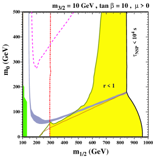
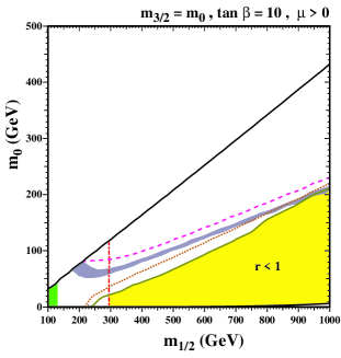
Figure 4: The $(m_{1/2},m_{0})$ planes for $\tan\beta=10,\mu>0$ and the choices (a) $m_{\tilde{G}}=10$ GeV, (b) $m_{\tilde{G}}=m_{0}$, assuming that the gravitino is the LSP [37]. In each panel, we show $m_{h}=114$ GeV calculated using FeynHiggs [38], as a near-vertical (red) dot-dashed line, the region excluded by $b\to s\gamma$ is darkly shaded(green), and the region where the NSP density before decay lies in the range $0.094<\Omega^{0}_{NSP}h^{2}<0.129$ is medium shaded (grey-blue). The (purple) dashed line is the contour where gravitinos produced in NSP decay have $\Omega_{3/2}h^{2}=0.129$, and the grey (khaki) solid line ($r=1$) is the constraint on NSP decays provided by Big-Bang nucleosynthesis and CMB observations. The light (yellow) shaded region is allowed by all the constraints. The contour where $m_{\chi}=m_{\tilde{\tau}_{1}}$ is shown as a (red) diagonal dotted line. Panel (a) shows as a black solid line the contour beyond which $\tau_{NSP}\mathrel{\raise 1.29167pt\hbox{$<$\kern-7.5pt\lower 4.30554pt\hbox{$\sim$}}}10^{4}$ s, a case not considered here. Panel (d) shows black lines to whose left the gravitino is no longer the LSP.

In this case, the constraint on the relic gravitino density from primordial thermal production is correspondingly weaker. For $\Omega_{\tilde{G}}\mathrel{\raise 1.29167pt\hbox{$<$\kern-7.5pt\lower 4.30554pt\hbox{$\sim$}}}0.1$ as required by the astrophysical cold dark matter density, and $Y_{\tilde{G}}\mathrel{\raise 1.29167pt\hbox{$>$\kern-7.5pt\lower 4.30554pt\hbox{$\sim$}}}10^{-11}\times(T_{RH}/10^{10}~{}{\rm GeV})$, so that the reheating temperature is bounded by [37]

$$T_{RH}\;\mathrel{\raise 1.29167pt\hbox{$<$\kern-7.5pt\lower 4.30554pt\hbox{$\sim$}}}10^{10}~{}{\rm GeV}\times\left(\frac{100~{}{\rm GeV}}{m_{\tilde{G}}}\right).$$ (63)

Although this is considerably larger than the bound in the case when the gravitino is not the lightest sparticle, it is still much lower than the expected inflaton sneutrino mass.

5.3 Implications for Leptogenesis

Some can be inferred from Fig. 3, where the regions of thermal and non-thermal leptogenesis are delineated [4]. If the lightest sneutrino were lighter than about $10^{10}$ GeV, there would be a small region where the gravitino LSP constraint (63) could be satisfied. However, the stronger gravitino NSP constraint is never compatible with thermal leptogenesis. Moreover, if the lightest sneutrino is responsible for inflation, with a mass $\sim 2\times 10^{13}$ GeV as estimated earlier, leptogenesis would have to be non-thermal, in both the gravitino LSP and NSP scenarios described above.

5.4 Implications for LFV

The hypothesis of sneutrino inflation constrains significantly the extra parameters in the seesaw model. One of the heavy singlet (s)neutrino masses is fixed at $\sim 2\times 10^{13}$ GeV and, in the simplest case, the other two must be heavier. Moreover, in order for the reheating temperature after inflation to be acceptably low, the couplings of the inflaton sneutrino must be quite small. Fig. 5 shows the implications for the LFV decays $\mu\to e\gamma$ and $\tau\to\mu\gamma$ [4]. In both cases, we see that the LFV decays are essentially independent of $T_{RH}$ once it is less than about $10^{12}$ GeV, so the predictions would be similar in the gravitino LSP and NSP scenarios decsribed above. Comparing the top and bottom bands in the first panel, we see that the branching ratio of $\mu\to e\gamma$ has considerable sensitivity to $\sin\theta_{13}$ and, comparing the bottom two bands, also to the mass $M_{3}$ of the heaviest singlet neutrino. In the second panel, we see that the branching ratio for $\tau\to\mu\gamma$ depends differently on $\sin\theta_{13}$ and is much more sensitive to $M_{3}$.

Figure 5: Calculations of BR$(\mu\to e\gamma)$ and BR$(\tau\to\mu\gamma)$ in the left and right panels, respectively [4]. Black points correspond to $\sin\theta_{13}=0.0$, $M_{2}=10^{14}$ GeV, and $5\times 10^{14}$ GeV $<M_{3}<5\times 10^{15}$ GeV. Red points correspond to $\sin\theta_{13}=0.0$, $M_{2}=5\times 10^{14}$ GeV and $M_{3}=5\times 10^{15}$ GeV, while green points correspond to $\sin\theta_{13}=0.1$, $M_{2}=10^{14}$ GeV, and $M_{3}=5\times 10^{14}$ GeV.

6 LFV IN DECOUPLING MODELS

Sneutrino inflation is one hypothesis motivating the (near-)decoupling of one heavy singlet sneutrino, which is also motivated by some flavour models of neutrino masses within the seesaw model [11]. In this Section, we explore in more detail the implications of such decoupling for LFV processes [5].

We may write the neutrino Yukawa coupling matrix in the general form

$$Y_{\nu}\;\propto M_{N}^{1/2}\Omega U_{\nu},$$ (64)

where $U_{\nu}$ is the MNS neutrino mixing matrix:

$${U}_{\nu} = \left(\matrix{c_{12}&s_{12}&s_{13}e^{-i\delta}\cr-\frac{s_{12}}{\sqrt{2}}+\dots&\frac{c_{12}}{\sqrt{2}}+\dots&{1\over\sqrt{2}}\cr{s_{12}\over\sqrt{2}}+\dots&-{c_{12}\over\sqrt{2}}+\dots&{1\over\sqrt{2}}}\right)$$ (65)

$$\cdot \mathrm{diag}(e^{i\phi_{1}},e^{i\phi_{2}},1),$$

where neutrino data suggest that $\sin^{2}\theta_{13}\sim 0.315$, the Majorana phases $\phi_{1,2}$ are unknown, and we consider two extreme hypotheses for $\theta_{13}$ and the CP-violating phase $\delta$ [5]:

$${\rm a):}\;\sin\theta_{13}=0,\;{\rm b):}\;\sin\theta_{13}=0.1,\delta=\frac{\pi}{2}.$$ (66)

Furthermore, we assume

$$m_{\nu_{1}}\ll m_{\nu_{2}}<m_{\nu_{3}},\;M_{1}\leq M_{2}<M_{3}.$$ (67)

Finally, we assume that one of the flavours (almost) decouples from the other two in the unknown matrix $\Omega$. The (almost) decoupled flavour may be any one of the three:

decoupling of $$N_{1} \Omega_{\nu}=\left(\begin{array}[]{ccc}1&0&0\\ 0&z&p\\ 0&\mp p&\pm z\end{array}\right)$$ (71)

decoupling of $$N_{2} \Omega_{\nu}=\left(\begin{array}[]{ccc}0&z&p\\ 1&0&0\\ 0&\mp p&\pm z\end{array}\right)$$ (75)

decoupling of $$N_{3} \Omega_{\nu}=\left(\begin{array}[]{ccc}0&z&p\\ 0&\pm p&\mp z\\ 1&0&0\end{array}\right)$$ (79)

where $z^{2}+p^{2}=1$. The first of these options was that explored in [4], and will be studied further here: the other options were discussed in [5].

To a good approximation, the LFV branching ratios for $\ell_{A}\to\ell_{B}+\gamma$ processes are proportional to the off-diagonal soft supersymmetry-breaking quantities $|{\tilde{m}}^{2}_{AB}|^{2}$, where in a leading-logarithmic approximation

$$\tilde{m}^{2}_{AB}\propto\Sigma_{C}(Y^{CA}_{\nu})^{*}\ln(m_{X}/M_{C})(Y^{CB}_{\nu})~{}.$$ (80)

This is a useful guide to understanding the results shown below, which are however based on calculations using the full one-loop renormalization-group equations.

6.1 $\tau\to\mu\gamma$

In the first decoupling pattern (71), we have [5]

$${\tilde{m}}^{2}_{AB}\,\approx\,\left[U_{\nu}^{33}U_{\nu}^{23\ast}\left(|z|^{2}+S|1-z^{2}|\right)\right.+$$

$$+ R\,U_{\nu}^{33}U_{\nu}^{22\ast}\left(Sz\sqrt{1-z^{2}}^{\ast}-z^{\ast}\sqrt{1-z^{2}}\right)+$$

$$+ R\,U_{\nu}^{32}U_{\nu}^{23\ast}\left(Sz^{\ast}\sqrt{1-z^{2}}-z\sqrt{1-z^{2}}^{\ast}\right)+$$

$$+ \left.R^{2}\,U_{\nu}^{32}U_{\nu}^{22\ast}\left(S|z|^{2}+|1-z^{2}|\right)\right],$$

where $R=\sqrt{m_{\nu_{2}}/m_{\nu_{3}}}\sim 0.41$ and $S$ gives the subleading contribution of the product $(Y_{\nu_{2A}})^{*}Y_{\nu_{2B}}$. The branching ratio does not depend strongly on the masses $M_{1}$ and $M_{2}$ and the Majorana phase $\phi_{1}$, as long as $M_{1}<M_{2}\ll M_{3}$, i.e., for $S\ll 1$. For illustration, we take $M_{3}=5\times 10^{14}$ GeV, $M_{2}=3\times 10^{13}$ GeV ($S\approx 0.1$) and $M_{1}=2\times 10^{13}$ GeV, consistent with inflation being driven by the lightest singlet sneutrino.

We see in Fig. 6 that the branching ratio for $\tau\to\mu\gamma$ does not vary greatly with $\phi_{2}$ and the phase of $z$, for representative choices of the other parameters and the two options (66) for $\theta_{13},\delta$. On the other hand, we see in Fig. 7 that the branching ratio for $\tau\to\mu\gamma$ does vary quite significantly with $|z|$ [5]. It would seem from these plots that $\tau\to\mu\gamma$ might have a branching ratio above $10^{-9}$, but before reaching this conclusion we must examine the model predictions for $\mu\to e\gamma$.

Figure 6: The branching ratio for $\tau\to\mu\gamma$ divided by a kinematic factor $f(m_{0},M_{1/2})$, $BR(\tau\to\mu\gamma)/f(m_{0},M_{1/2})$, as a function of $\phi_{2}$ for the choices of $\theta_{13},\delta$ in (66), $|z|=1/\sqrt{2}$, $\tan\beta=10$ and $A_{0}=0$ [5]. Dotted, dashed and solid lines correspond to $\arg z=0,\pi/4,\pi/2$, respectively.

Figure 7: Extremal values of $BR(\tau\to\mu\gamma)/f(m_{0},M_{1/2})$ as a function of $|z|$ for the choices of $\theta_{13},\delta$ in (66), $\tan\beta=10$ and $A_{0}=0$ [5]. Dotted, dashed and solid lines correspond to $\arg z=0,\pi/4,\pi/2$, respectively.

6.2 $\mu\to e\gamma$

The quantity ${\tilde{m}}^{2}_{L_{21}}$ relevant for $\mu\to e\gamma$ decay can be approximated by:

$${\tilde{m}}^{2}_{L_{21}}\propto$$ (82)

$$\left[RU_{\nu}^{A3}U_{\nu}^{12*}\left(Sz\sqrt{1-z^{2}}^{\ast}-z^{\ast}\sqrt{1-z^{2}}\right)\right.$$

$$+ R^{2}U_{\nu}^{A2}U_{\nu}^{12\ast}\left(S|z|^{2}+|1-z^{2}|\right)+$$

$$+ \left.U_{\nu}^{A3}U_{\nu}^{13\ast}\left(|z|^{2}+S|1-z^{2}|\right)\right],$$

where we use again the decoupling texture (71) [5]. As seen in Fig. 8, $\mu\to e\gamma$ exhibits a stronger dependence on $\phi_{2}$ than does $\tau\to\mu\gamma$ and, as seen in Fig. 9, it exhibits cancellations for some specific values of $|z|$ and the other parameters. This is just as well, because the prediction for the branching ratio of $\mu\to e\gamma$ rises above the present experimental limit of $1.2\times 10^{-11}$ for generic values of the parameters. However, even in the narrow regions where there is a cancellation, the branching ratio of $\mu\to e\gamma$ generally exceeds $10^{-13}$, within the sensitivity of the ongoing experiment at PSI. Unfortunately, referring back to Fig. 7, we see that the regions where $\mu\to e\gamma$ is acceptably rare do not have large branching ratios for $\tau\to\mu\gamma$. This is a pity, as the ratio of the two decays would provide valuable information about a complex parameter of the seesaw model that is inaccessible in neutrino oscillation experiments [5].

Figure 8: $BR(\mu\to e\gamma)/f(m_{0},M_{1/2})$ as a function of $\phi_{2}$ for the choices of $\theta_{13},\delta$ in (66), $|z|=1/\sqrt{2}$, $\tan\beta=10$ and $A_{0}=0$ [5]. Dotted, dashed and solid lines correspond to $\arg z=0$, $\pi/4$ and $\pi/2$, respectively.

Figure 9: Extremal values of $BR(\mu\to e\gamma)/f(m_{0},M_{1/2})$ as a function of $|z|$ for the choices of $\theta_{13},\delta$ in (66), $\tan\beta=10$ and $A_{0}=0$ [5]. Dotted, dashed and solid lines correspond to $\arg z=0$, $\pi/4$ and $\pi/2$, respectively.

6.3 $\tau\to e\gamma$

We consider finally the decay $\tau\to e\gamma$. Within the decoupling texture (71), this has a dependence on $\phi_{2}$ that is quite strong but opposite to that of $\tau\to\mu\gamma$. The branching ratio is generally smaller than that for $\tau\to\mu\gamma$, as seen in Fig. 10, particularly in the cancellation regions [5].

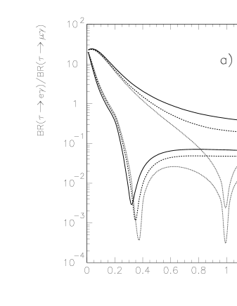
Figure 10: The extremal values of $BR(\tau\to e\gamma)/BR(\tau\to\mu\gamma)$ as a function of $|z|$ for the choices of $\theta_{13},\delta$ in (66), $\tan\beta=10$ and $A_{0}=0$ [5]. Dotted, dashed and solid lines correspond to $\arg z=0$, $\pi/4$ and $\pi/2$, respectively.

7 CONCLUSIONS

The contemporary techno-folk singer Moby tells us that ‘We are all made of stars’. Perhaps this is a reference to astrophysical nucleosynthesis? In contrast, my main message in this talk is that ‘We are all made of neutrinos’, not just in the sense of leptogenesis, but also in the sense that the overall size, age, flatness and entropy are all due to neutrinos, via cosmological inflation. Moreover, this hypothesis enables some testable predictions to made for the radiative charged-lepton decays $\mu\to e\gamma$, $\tau\to\mu\gamma$ and $\tau\to e\gamma$.

References

- [1] C. L. Bennett et al., Astrophys. J. Suppl. 148 (2003) 1 [arXiv:astro-ph/0302207]; D. N. Spergel et al., Astrophys. J. Suppl. 148 (2003) 175 [arXiv:astro-ph/0302209]; H. V. Peiris et al., Astrophys. J. Suppl. 148 (2003) 213 [arXiv:astro-ph/0302225].
- [2] H. Murayama, H. Suzuki, T. Yanagida and J. Yokoyama, Phys. Rev. Lett. 70 (1993) 1912.
- [3] H. Murayama, H. Suzuki, T. Yanagida and J. Yokoyama, Phys. Rev. D50 (1994) 2356 [arXiv:hep-ph/9311326]; see also K. Hamaguchi, H. Murayama and T. Yanagida, Phys. Rev. D65 (2002) 043512 [hep-ph/0109030].
- [4] J. R. Ellis, M. Raidal and T. Yanagida, Phys. Lett. B581 (2004) 9 [arXiv:hep-ph/0303242].
- [5] P. H. Chankowski, J. Ellis, S. Pokorski, M. Raidal and K. Turzynski, arXiv:hep-ph/0403180.
- [6] D. H. Lyth and A. Riotto, Phys. Rept. 314, 1 (1999) [arXiv:hep-ph/9807278]; W. H. Kinney, Phys. Rev. D 58, 123506 (1998) [arXiv:astro-ph/9806259], and arXiv:astro-ph/0301448.
- [7] J. A. Casas and A. Ibarra, Nucl. Phys. B618 (2001) 171 [arXiv:hep-ph/0103065].
- [8] J. R. Ellis, J. Hisano, S. Lola and M. Raidal, Nucl. Phys. B621 (2002) 208 [arXiv:hep-ph/0109125].
- [9] J. R. Ellis and M. Raidal, Nucl. Phys. B 643 (2002) 229 [arXiv:hep-ph/0206174].
- [10] J. R. Ellis, J. E. Kim and D. V. Nanopoulos, Phys. Lett. B145 (1984) 181; J. R. Ellis, D. V. Nanopoulos and S. Sarkar, Nucl. Phys. B259 (1985) 175; J. R. Ellis, D. V. Nanopoulos, K. A. Olive and S. J. Rey, Astropart. Phys. 4 (1996) 371; M. Kawasaki and T. Moroi, Prog. Theor. Phys. 93 (1995) 879; T. Moroi, Ph.D. thesis, arXiv:hep-ph/9503210.
- [11] S.F. King, Phys. Lett. B439 (199) 350 and Nucl. Phys. B562 (1999) 57; S. Davidson and S.F. King, Phys. Lett. B445 (1998) 191; Q. Shafi and Z. Tavarkiladze, Phys. Lett. B451 (1999) 129; S.F. King, Nucl. Phys. B576 (2000) 85; S.F. King and G.G. Ross, Phys. Lett. B520 (2001) 243.
- [12] A. H. Guth, Phys. Rev. D 23 (1981) 347.
- [13] E. R. Harrison, Phys. Rev. D 1 (1970) 2726; Y. B. Zeldovich, Mon. Not. Roy. Astron. Soc. 160 (1972) 1.
- [14] A. D. Linde, Phys. Lett. B 129 (1983) 177.
- [15] V. Barger, H. S. Lee and D. Marfatia, arXiv:hep-ph/0302150.
- [16] M. Gell-Mann, P. Ramond and R. Slansky, in Proceedings of the Supergravity Stony Brook Workshop, New York, 1979 (eds. P. van Nieuvenhuizen and D.Z. Freedman, North-Holland, Amsterdam); T. Yanagida, in Proceedings of the Workshop on Unified Theories and Baryon Number in the Universe, Tsukuba, Japan, 1979 (eds. A. Sawada and A. Sugamoto, KEK Report No. 79-18, Tsukuba).
- [17] P. H. Frampton, S. L. Glashow and T. Yanagida, Phys. Lett. B548 (2002) 119 [arXiv:hep-ph/0208157].
- [18] T. Endoh, S. Kaneko, S. K. Kang, T. Morozumi and M. Tanimoto, arXiv:hep-ph/0209020.
- [19] J. R. Ellis, J. S. Hagelin, S. Kelley and D. V. Nanopoulos, Nucl. Phys. B 311 (1988) 1.
- [20] J. R. Ellis, M. E. Gómez, G. K. Leontaris, S. Lola and D. V. Nanopoulos, Eur. Phys. J. C 14 (2000) 319.
- [21] J. R. Ellis, M. K. Gaillard and D. V. Nanopoulos, Nucl. Phys. B 109 (1976) 213.
- [22] M. Kobayashi and T. Maskawa, Prog. Theor. Phys. 49 (1973) 652.
- [23] Z. Maki, M. Nakagawa and S. Sakata, Prog. Theor. Phys. 28 (1962) 870.
- [24] A. De Rújula, M.B. Gavela and P. Hernández, Nucl. Phys. B 547 (1999) 21 [arXive:hep-ph/9811390].
- [25] F. Borzumati and A. Masiero, Phys. Rev. Lett. 57 (1986) 961.
- [26] S. Davidson and A. Ibarra, JHEP 0109 (2001) 013 [arXiv:hep-ph/0104076].
- [27] J. R. Ellis, J. Hisano, M. Raidal and Y. Shimizu, Phys. Lett. B528 (2002) 86 [arXiv:hep-ph/0111324].
- [28] J. R. Ellis, J. Hisano, M. Raidal and Y. Shimizu, Phys. Rev. D66 (2002) 115013 [arXiv:hep-ph/0206110].
- [29] M. Fukugita and T. Yanagida, Phys. Lett. B 174 (1986) 45.
- [30] J. R. Ellis and D. V. Nanopoulos, Phys. Lett. B 110 (1982) 44; R. Barbieri and R. Gatto, Phys. Lett. B 110 (1982) 211.
- [31] A. Masiero and O. Vives, New J. Phys. 4 (2002) 4.
- [32] C. Jarlskog, Phys. Rev. Lett. 55 (1985) 1039; Z. Phys. C 29 (1985) 491.
- [33] G. F. Giudice, A. Notari, M. Raidal, A. Riotto and A. Strumia, arXiv:hep-ph/0310123.
- [34] R. Cyburt, J. R. Ellis, B. D. Fields and K. A. Olive, arXiv:astro-ph/0211258.
-
[35]
M. Bolz, A. Brandenburg and
W. Buchmüller, Nucl. Phys. B606 (2001) 518. - [36] M. Kawasaki, K. Kohri and T. Moroi, arXiv:astro-ph/0402490.
- [37] J. Ellis, K. A. Olive, Y. Santoso and V. C. Spanos, arXiv:hep-ph/0312262.
- [38] S. Heinemeyer, W. Hollik and G. Weiglein, Comput. Phys. Commun. 124 (2000) 76 [arXiv:hep-ph/9812320]; S. Heinemeyer, W. Hollik and G. Weiglein, Eur. Phys. J. C 9 (1999) 343 [arXiv:hep-ph/9812472].