SISSA 22/2004/EP
hep-ph/0403236

Type II See–Saw Mechanism, Deviations from Bimaximal Neutrino Mixing and Leptogenesis

Abstract

A possible interplay of both terms in the type II see–saw formula is illustrated by presenting a novel way to generate deviations from exact bimaximal neutrino mixing. In type II see–saw mechanism with dominance of the non–canonical $SU(2)_{L}$ triplet term, the conventional see–saw term can naturally give a small contribution to the neutrino mass matrix. If the triplet term corresponds to the bimaximal mixing scheme in the normal hierarchy, the small contribution of the conventional see–saw term naturally generates non–maximal solar neutrino mixing. Atmospheric neutrino mixing is also reduced from maximal, corresponding to $1-\sin^{2}2\theta_{23}$ of order 0.01. Also, small but non–vanishing $U_{e3}$ of order 0.001 is obtained. It is also possible that the $\Delta m^{2}$ responsible for solar neutrino oscillations is induced by the small conventional see–saw term. Larger deviations from zero $U_{e3}$ and from maximal atmospheric neutrino mixing are then expected. This scenario links the small ratio of the solar and atmospheric $\Delta m^{2}$ with the deviation from maximal solar neutrino mixing. We comment on leptogenesis in this scenario and compare the contributions to the decay asymmetry of the heavy Majorana neutrinos as induced by themselves and by the triplet.

1 Introduction

The bimaximal neutrino mixing scheme [1] is esthetically and theoretically very appealing but suffers — as many simple frameworks — from the fact that Nature did not realize it with perfect accuracy. In this particular case, solar neutrino mixing is not maximal. Recent data as collected by the SNO salt phase [2] and by the KamLAND [3] experiment shows that $\tan^{2}\theta_{\rm sol}<1$ at more than 5$\sigma$ [2]. Nevertheless, the (close to) maximal atmospheric neutrino mixing and the smallness of $U_{e3}$ can lead one to believe that Nature presumably started with bimaximal mixing and that the underlying symmetry (one could imagine, e.g., flavor symmetries such as $L_{e}-L_{\mu}-L_{\tau}$ [4]) was somehow broken to yield the observed phenomenology. There are several approaches trying to explain deviations from bimaximal neutrino mixing, e.g., from charged lepton mixing [5, 6, 7, 8], from radiative corrections [9] or from breaking of symmetries [11].

The primary goal of all those approaches is to generate non–maximal solar neutrino mixing, which can be parametrized through a small parameter $\lambda\sim 0.2$ as [7]

$$U_{e2}=\sqrt{\frac{1}{2}}~{}(1-\lambda)~{}.$$ (1)

Note that the parameter $\lambda$ is very similar to the Cabibbo angle: $\lambda\simeq\theta_{C}$ [7]. When one starts from bimaximal neutrino mixing and introduces some deviation to generate non–maximal solar neutrino mixing, usually also $U_{e3}$ and atmospheric mixing will deviate from their “bimaximal” values. Thus, those additional deviations will be proportional to some power of $\lambda$, depending on the model. A useful parametrization taking into account this fact is [7]

$$U_{e3}=A_{\nu}~{}\lambda^{n}\mbox{ and }U_{\mu 3}=\sqrt{\frac{1}{2}}~{}(1-B_{\nu}~{}\lambda^{m})~{}e^{i\delta},$$ (2)

where the integer numbers $m,n$ and the order one numbers $A_{\nu},B_{\nu}$ are to be chosen according to the numerical values of $U_{e3}$ and $U_{\mu 3}$.

Numerically, it turns out that the phenomenologically very interesting ratio $R$ of the solar and atmospheric $\Delta m^{2}$ is of order $\lambda^{2}$ [7]. This can be interpreted in the sense that both the deviation from bimaximal neutrino mixing and the small ratio $R$ have the same origin. Hence, it would be interesting to have a scenario in which one starts from zero $\Delta m^{2}_{\odot}$ together with bimaximal mixing and ends up with the observed phenomenology of non–maximal solar neutrino mixing and a small ratio of the solar and atmospheric $\Delta m^{2}$.

In this note we shall try to reason that in type II see–saw models, i.e.,

$$m_{\nu}=m_{L}-m_{D}^{T}\,M_{R}^{-1}\,m_{D}~{},$$ (3)

with dominance of the $SU(2)_{L}$ triplet term [12] $m_{L}$, the conventional see–saw term
$m_{D}^{T}\,M_{R}^{-1}\,m_{D}$ can naturally give a small correction to $m_{L}$. Starting with a structure of $m_{L}$ which corresponds to bimaximal mixing in the normal mass hierarchy and using the natural assumptions $m_{L}\propto M_{R}$ as well as hierarchical $m_{D}$, one can easily obtain non–maximal solar neutrino mixing while keeping the atmospheric neutrino mixing close to maximal and generating small but non–vanishing $U_{e3}$. In addition, it is also possible to generate non–vanishing $\Delta m^{2}_{\odot}$ via the small conventional see–saw contribution. This is then a scenario linking the deviations from bimaximal mixing and the small $R$.

We shall not speculate about particular models in which such a scenario arises but rather investigate its consequences on neutrino phenomenology. The simple situation from which we start, the illustration of an interesting interplay of both terms in the type II see–saw formula and the possibility to link the small ratio $R$ with the deviation from bimaximal neutrino mixing justifies this approach.

We also consider leptogenesis as realized through heavy Majorana neutrino decays and compare for the first time in a concrete situation the contributions to the decay asymmetry induced by diagrams involving virtual Majorana neutrinos and the $SU(2)_{L}$ triplet.

The paper is organized as follows. In Section 2 we briefly describe the phenomenological and theoretical framework in which we work. We consider the $CP$ conserving case in Section 3 and the $CP$ violating one in Section 4, which includes general considerations, the application to the specific case we are interested in, and leptogenesis. Finally, Section 5 summarizes and concludes this work.

2 Framework

The light neutrino Majorana mass matrix $m_{\nu}$ is given by

$$m_{\nu}=U^{\ast}\,\,m_{\nu}^{\rm diag}\,U^{\dagger}~{}.$$ (4)

Here $m_{\nu}^{\rm diag}$ is a diagonal matrix containing the light neutrino mass eigenstates $m_{i}$. Mixing is described by $U$, the unitary Pontecorvo–Maki–Nagakawa–Sakata [13] lepton mixing matrix, which can be parametrized as

$$\begin{array}[]{c}U=\left(\begin{array}[]{ccc}c_{12}c_{13}&s_{12}c_{13}&s_{13}e^{-i\delta}\\[5.69046pt] -s_{12}c_{23}-c_{12}s_{23}s_{13}e^{i\delta}&c_{12}c_{23}-s_{12}s_{23}s_{13}e^{i\delta}&s_{23}c_{13}\\[5.69046pt] s_{12}s_{23}-c_{12}c_{23}s_{13}e^{i\delta}&-c_{12}s_{23}-s_{12}c_{23}s_{13}e^{i\delta}&c_{23}c_{13}\\ \end{array}\right){\rm diag}(1,e^{i\alpha},e^{i(\beta+\delta)})\,,\end{array}$$ (5)

where $c_{ij}=\cos\theta_{ij}$, $s_{ij}=\sin\theta_{ij}$ and three physical phases $\alpha,\beta$ and $\delta$ are present. We shall work throughout this note in a basis in which the charged lepton mass matrix $m_{\ell}$ is real and diagonal.

The ranges of values of the three neutrino mixing angles, which are allowed at 1(3)$\sigma$ by the current solar and atmospheric neutrino data and by the data from the reactor antineutrino experiments CHOOZ and KamLAND, read [14, 15]:

$$\begin{array}[]{c}0.35~{}(0.27)\leq\tan^{2}\theta_{\rm sol}\equiv\tan^{2}\theta_{12}\leq 0.52~{}(0.72)~{},\\[8.5359pt] |U_{e3}|^{2}=\sin^{2}\theta_{13}<0.029~{}(0.074)~{},\\[5.69046pt] \sin^{2}2\theta_{\rm atm}\equiv\sin^{2}2\theta_{23}\geq 0.95~{}(0.85)~{}.\end{array}$$ (6)

Zero $U_{e3}$ and maximal atmospheric neutrino mixing are still allowed by the data, whereas maximal solar neutrino mixing is ruled out by more than 5$\sigma$ [2, 14].

For bimaximal neutrino mixing [1] one has $\theta_{12}=\theta_{23}=\pi/4$ and $\theta_{13}=0$. The corresponding neutrino mass matrix in case of $CP$ conservation then reads:

$$\begin{array}[]{c}m_{\nu}^{\rm bimax}=\left(\begin{array}[]{ccc}\displaystyle A&B&-B\\[5.69046pt] \displaystyle\cdot&\displaystyle D+\frac{A}{2}&\displaystyle D-\frac{A}{2}\\[8.5359pt] \displaystyle\cdot&\cdot&\displaystyle D+\frac{A}{2}\end{array}\right)~{},\end{array}$$ (7)

where

$$A=\frac{m_{1}^{0}+m_{2}^{0}}{2}~{},~{}B=\frac{m_{2}^{0}-m_{1}^{0}}{2\,\sqrt{2}}~{},~{}D=\frac{m_{3}^{0}}{2}~{}.$$ (8)

In case of $CP$ conservation, different relative signs of the mass states $m_{i}^{0}$ are possible.

On the theoretical side, the most general form [16, 17] for the light neutrino mass matrix is the type II see–saw formula

$$m_{\nu}=m_{L}-m_{D}^{T}\,M_{R}^{-1}\,m_{D}\equiv m_{\nu}^{II}+m_{\nu}^{I}~{},$$ (9)

where the second term $m_{\nu}^{I}$ is the conventional ordinary see–saw term. The first term is absent or suppressed in the major part of the theoretical works dedicated to neutrino physics. It can arise, for instance, in a large class of $SO(10)$ models in which the $B-L$ symmetry is broken by a 126 Higgs field [18]. The relevant Lagrangian, which gives rise to the mass matrix (9) is

$${\cal L}=\frac{1}{2}~{}(\nu_{L}^{T})~{}C^{-1}~{}m_{L}~{}\nu_{L}+\frac{1}{2}~{}(N_{R}^{T})~{}C^{-1}~{}M_{R}~{}N_{R}+\overline{N_{R}}~{}m_{D}~{}\ell_{L}+\overline{\ell_{L}}~{}m_{\ell}~{}\ell_{R}+h.c.,$$ (10)

where $N_{R}$ ($\nu_{L}$) are the right–handed (left–handed) Majorana neutrinos and $\ell_{L,R}$ the charged leptons. In recent time, the situation in which the $m_{L}$ term dominates $m_{\nu}$ has gathered some attention because in certain $SO(10)$ models atmospheric neutrino mixing is a natural outcome of this dominance [18].

In usual left–right symmetric theories $m_{L}$ and $M_{R}$ are proportional to the vacuum expectation values (vevs) of the electrically neutral components of scalar Higgs triplets, i.e., $m_{L}=f_{L}~{}v_{L}$ and $v_{R}=f_{R}~{}v_{R}$, where $v_{L,R}$ denotes the vevs and $f_{L,R}$ are symmetric $3\times 3$ matrices. By acquiring the vev $v_{R}$, breaking of $SU(2)_{L}\times SU(2)_{R}\times U(1)_{B-L}$ to $SU(2)_{L}\times U(1)_{Y}$ is achieved [17]. The left–right symmetry demands the presence of both $m_{L}$ and $M_{R}$, and in addition it holds $f_{R}=f_{L}$. Whether $m_{\nu}^{I}$ or $m_{\nu}^{II}$ dominates $m_{\nu}$ depends on the details of the model.

Actually, in the class of models we refer to, there is a Higgs bi–doublet which gives rise to two Dirac mass terms. We shall assume for simplicity that only one of them plays a role for the lepton masses and later on for leptogenesis. This will be possible if, e.g., the coupling of one of the two $SU(2)_{L}$ doublets in the bi–doublet is suppressed by a very small vev.

Since left–right symmetry implies $f_{R}=f_{L}\equiv f$, the following relations hold:

$$m_{L}=\frac{v_{L}}{v_{R}}\,M_{R}~{}\mbox{ with }v_{R}\,v_{L}=\gamma\,v^{2}~{},$$ (11)

where $v$ is the SM Higgs vev and $\gamma$ a model dependent factor of order one. Thus, the neutrino mass matrix can be written as

$$m_{\nu}=v_{L}\left(f-\frac{1}{\gamma\,v^{2}}~{}m_{D}^{T}~{}f^{-1}~{}m_{D}\right)~{}.$$ (12)

The relation Eq. (11) ensures that the type II see–saw mechanism [17] works, which sets the scale of neutrino masses by the vev $v_{L}$, where $v_{L}\propto 1/v_{R}$ with $v_{R}\gg m_{D}\gg v_{L}$. See [19] for a recent review and further references. Knowing the eigenvalues $m_{i}^{0}$ of $m_{L}$ will give the heavy Majorana neutrino masses $M_{i}$ through the relation

$$M_{i}=\frac{v_{R}}{v_{L}}\,m_{i}^{0}\simeq 3\cdot 10^{10}\,\frac{1}{\gamma}\left(\frac{v_{R}}{10^{15}\,\rm GeV}\right)^{2}\,\left(\frac{m_{i}^{0}}{10^{-3}\,\rm eV}\right)\,{\rm GeV}~{}.$$ (13)

In particular, the spectrum of the light Majorana masses in $m_{L}$ is identical to the spectrum of the heavy ones in $M_{R}$. The absence of $m_{\nu}^{I}$ would mean that the light neutrinos $\nu_{i}$, whose oscillations are currently measured, would have masses $m_{i}^{0}$. The mass spectrum of those neutrinos would then fix the mass spectrum of the heavy ones. See, e.g., [20, 21] for such a situation. In the remainder of the paper we shall discuss a small contribution of $m_{\nu}^{I}$ to $m_{\nu}$ and thus the spectrum of the light (oscillating) neutrinos will be slightly different from the one of the heavy Majorana neutrinos.

Now we shall assume that the triplet term $m_{L}$ in Eq. (9) corresponds to $m_{\nu}^{\rm bimax}$. In order to obtain the physical light neutrinos one has to calculate the inverse matrix of $M_{R}$; using Eq. (11) and $m_{L}=m_{\nu}^{\rm bimax}$ one finds:

$$\begin{array}[]{c}M_{R}^{-1}=\frac{\displaystyle v_{L}}{\displaystyle v_{R}}~{}m_{L}^{-1}=\frac{\displaystyle v_{L}}{\displaystyle v_{R}}~{}\left(\begin{array}[]{ccc}\tilde{A}&\tilde{B}&-\tilde{B}\\[8.5359pt] \cdot&\tilde{D}+\frac{\displaystyle\tilde{A}}{\displaystyle 2}&\tilde{D}-\frac{\displaystyle\tilde{A}}{\displaystyle 2}\\[8.5359pt] \cdot&\cdot&\tilde{D}+\frac{\displaystyle\tilde{A}}{\displaystyle 2}\\[8.5359pt] \end{array}\right)~{},\end{array}$$ (14)

where

$$\tilde{A}=\frac{A}{A^{2}-2B^{2}}~{},~{}\tilde{B}=\frac{B}{2B^{2}-A^{2}}~{},~{}\tilde{D}=\frac{1}{4D}~{}.$$ (15)

Thus, $M_{R}^{-1}$ has a similar structure as $m_{L}$ or $m_{\nu}^{\rm bimax}$ in Eq. (7). We shall assume in the following a normal hierarchical mass spectrum, i.e., $(m_{3}^{0})^{2}\gg(m_{1,2}^{0})^{2}$. This has the advantage that radiative corrections have only weak effects [22].

Now suppose that in the type II see–saw formula the term $m_{L}$ dominates. Furthermore, $m_{D}$ shall be hierarchical, i.e.,

$$m_{D}\simeq{\rm diag}(0,0,m)~{},$$ (16)

which is a very natural assumption, since $m_{D}$ is expected to be connected to the known fermion masses, which all display a very hierarchical mass spectrum. Then, from Eq. (9) one finds that the effect of the conventional see–saw term is a small contribution to the 33 entry of $m_{L}$ given by

$$s\equiv(m_{D}^{T}\,M_{R}^{-1}\,m_{D})_{33}\simeq v_{L}^{2}~{}\frac{m^{2}}{4\gamma\,v^{2}}\left(\frac{1}{m_{1}^{0}}+\frac{1}{m_{2}^{0}}+\frac{2}{m_{3}^{0}}\right)~{}.$$ (17)

It is the main observation of the present study that this term can generate the observed sizable deviation from maximal solar neutrino mixing while at the same time also pulling $\theta_{\rm atm}$ and $U_{e3}$ away from their extreme “bimaximal values” $\pi/4$ and zero, respectively.

The possible importance of this term in the class of models under consideration has been noted for the first time in [24]. Typically, in these $SO(10)$ inspired models, it holds that $m\simeq v$, i.e., the Dirac mass matrix is related to the up–quark mass matrix. For smaller Dirac masses, i.e., when $m_{D}$ is related to the down quarks or charged leptons, $m_{L}$ receives negligible corrections from the conventional see–saw term [20]. If however $m\simeq v$, then we can estimate this term as

$$s\simeq\frac{0.1}{4\gamma}\left(\frac{v_{L}}{10^{-2}~{}\rm eV}\right)^{2}\left(\frac{10^{-3}~{}\rm eV}{m_{1}^{0}}\right)~{}{\rm eV}~{},$$ (18)

where again hierarchical $m_{i}^{0}$ were assumed. A similar formula will hold when an inverted hierarchy with a non–zero smallest mass $m_{3}^{0}$ is present. Also, many non–singular mass matrices $M_{R}$ with hierarchical Dirac mass matrix will have the 33 entry as the leading term and can be cast in the form (18). For definiteness and the sake of simplicity, we shall stick to our left–right symmetry induced relation $m_{L}\propto M_{R}$. Naturally, for our reference values $m_{1}^{0}=10^{-3}$ eV and $v_{L}=10^{-2}$ eV, the order of $s$ can be — without varying $\gamma$ within more than one order of magnitude — given by the scale of neutrino masses $\sqrt{\mbox{$\Delta m^{2}_{\odot}$}}$ or $\sqrt{\mbox{$\Delta m^{2}_{\rm A}$}}$. The same is true for the case when the first two terms in Eq. (17) cancel each other, which will be of interest later on. Then it holds $s\simeq 0.01/(2\gamma)\,(v_{L}/10^{-2}\,{\rm eV})^{2}\,(10^{-2}\,{\rm eV}/m_{3}^{0})$ eV.

Realistic Dirac mass matrices contain of course more than one non–vanishing entry. It is useful to parametrize $m_{D}$ in terms of a small parameter $\epsilon_{D}$, e.g.,

$$m_{D}\simeq m\left(\begin{array}[]{ccc}0&a\,\epsilon_{D}^{3}&0\\[8.5359pt] b\,\epsilon_{D}^{3}&\epsilon_{D}^{2}&c\,\epsilon_{D}^{2}\\[8.5359pt] 0&d\,\epsilon_{D}^{2}&1\end{array}\right)~{},$$ (19)

where $a,b,c,d$ are of order one and we may take $\epsilon_{D}\simeq 0.07$ in order to reproduce a realistic up–quark mass ratio with this matrix. The conventional see–saw term implied by this Dirac mass matrix will have the following leading form:

$$m_{D}^{T}~{}M_{R}^{-1}~{}m_{D}\sim s\left(\begin{array}[]{ccc}\epsilon_{D}^{6}&\epsilon_{D}^{5}&\epsilon_{D}^{3}\\[5.69046pt] \cdot&\epsilon_{D}^{4}&\epsilon_{D}^{2}\\[5.69046pt] \cdot&\cdot&1\end{array}\right)~{},$$ (20)

which has only little effect on the results to be obtained for $m_{D}\simeq{\rm diag}(0,0,m)$.

3 $CP$ conservation

3.1 General case

We can easily diagonalize the mass matrix (7) when the term $s$ from Eq. (17) is subtracted from its 33 entry and the magnitude of $s$ is of order $D$ or smaller. One finds for the masses

$$m_{3}\simeq 2D-\frac{s}{2}~{},~{}m_{1,2}\simeq A-\frac{s}{4}\mp\sqrt{2\,B^{2}+\frac{s^{2}}{16}}~{},$$ (21)

which for $s\rightarrow 0$ reproduces $m_{i}=m_{i}^{0}$. Using Eq. (13), one could calculate the heavy Majorana neutrino masses. The atmospheric and solar $\Delta m^{2}$ read

$$\begin{array}[]{c}\mbox{$\Delta m^{2}_{\odot}$}=m_{2}^{2}-m_{1}^{2}\simeq\sqrt{2B^{2}+\frac{\displaystyle s^{2}}{\displaystyle 16}}~{}(4A-s)~{},\\[5.69046pt] \mbox{$\Delta m^{2}_{\rm A}$}=m_{3}^{2}-m_{2}^{2}\simeq 4D^{2}-(A^{2}+2B^{2})-s~{}\left(2D-A-\frac{\displaystyle s}{\displaystyle 8}\right)-\frac{1}{2}~{}\mbox{$\Delta m^{2}_{\odot}$}~{}.\end{array}$$ (22)

The mixing angles are given by

$$\begin{array}[]{c}\tan 2\theta_{23}\simeq\frac{\displaystyle 2D-A}{\displaystyle s}~{},~{}\tan 2\theta_{12}\simeq 4\sqrt{2}\,\frac{\displaystyle B}{\displaystyle s}~{}\left(1+\frac{\displaystyle s}{\displaystyle 2D-A}\right),{}\\[5.69046pt] \tan 2\theta_{13}\simeq\sqrt{2}\,\frac{\displaystyle B}{\displaystyle s}~{}\frac{\displaystyle s}{\displaystyle 2D-A}\frac{\displaystyle s}{\displaystyle 2D-A-s/2}~{}.\end{array}$$ (23)

Bimaximal mixing is obtained — as it should be — for $s=0$. Non–maximal solar neutrino mixing implies automatically non–maximal atmospheric neutrino mixing and non–zero $U_{e3}$. From the expression for $\theta_{12}$ and assuming hierarchical $m_{i}^{0}$ one obtains that $|s|\sim|m_{2}^{0}|\sim\sqrt{\mbox{$\Delta m^{2}_{\odot}$}}$ in order to reproduce the observations. From the expression for $\theta_{23}$ and assuming again hierarchical $m_{i}^{0}$ it follows that $m_{3}^{0}\simeq\sqrt{\mbox{$\Delta m^{2}_{\rm A}$}}\mathrel{\hbox to0.0pt{\raise 2.20013pt\hbox{$>$}\hss}{\lower 2.20013pt\hbox{$\sim$}}}2.4\,(3,4.4)\,s$ for $\sin^{2}2\theta_{23}>0.85\,(0.9,0.95)$. With these values $\Delta m^{2}_{\rm A}$ is basically not affected by the conventional see–saw term. Also it holds that $m_{3}\simeq m_{3}^{0}$ and hence the mass of the heaviest Majorana neutrino is proportional to the mass of the heaviest of the light physical neutrinos: $M_{3}\simeq v_{R}/v_{L}\,m_{3}\simeq v_{R}/v_{L}\,\sqrt{\mbox{$\Delta m^{2}_{\rm A}$}}$. The lightest heavy Majorana masses $M_{1,2}$ show however sizable deviations from $v_{R}/v_{L}\,m_{1,2}$.

A useful parameter to describe the deviations from bimaximal mixing can be defined via [7] $U_{e2}=\sqrt{1/2}~{}(1-\lambda)$, where $\lambda\simeq 0.22$ for typical best–fit points. In our framework one finds from the above expression for $\tan 2\theta_{12}$ that to leading order $\lambda\simeq\sqrt{2}/16~{}s/B$. The other two deviations from bimaximal mixing can be described via Eq. (2); the appropriate powers of $\lambda$ are $U_{e3}\simeq A_{\nu}~{}\lambda^{4}$ and $|U_{\mu_{3}}|\simeq\sqrt{1/2}~{}(1-B_{\nu}~{}\lambda^{2})$, where $A_{\nu}$ and $B_{\nu}$ are of order one and are functions of $A,B$ and $D$. Note that $\lambda\propto s$, quantifying again that it is the small contribution $s$ of the conventional see–saw term that is responsible for the deviation from bimaximal mixing.

Eq. (23) and the fact that $2D\gg A,s/2$ can be used to obtain an interesting correlation of neutrino mixing observables:

$$|U_{e3}|\simeq\frac{1}{4}\,\frac{\tan\theta_{12}}{1-\tan^{2}\theta_{12}}\,\frac{1-\sin^{2}2\theta_{23}}{\sin^{2}2\theta_{23}}~{}.$$ (24)

The larger the deviation from maximal atmospheric neutrino mixing and the larger $\tan^{2}\theta_{12}$, the more sizable becomes $U_{e3}$.

Note that, though the mixing angles and the mass states are altered, the $ee$ entry of $m_{\nu}$ (the so-called effective Majorana mass), which is in principle measurable in neutrinoless double beta–decay experiments [25], is not changed by the procedure. We can express, however, the effective mass $\mbox{$\langle m\rangle$}\equiv A$ through $s$ and the neutrino mixing parameters, e.g.,

$$\mbox{$\langle m\rangle$}\simeq\sqrt{\mbox{$\Delta m^{2}_{\rm A}$}}-s\frac{\sin 2\theta_{23}}{\sqrt{1-\sin^{2}2\theta_{23}}}~{}.$$ (25)

Both terms can be sizable, but are subtracted so that small $\mbox{$\langle m\rangle$}\sim m_{2}^{0}\sim\sqrt{\mbox{$\Delta m^{2}_{\odot}$}}$ is obtained.

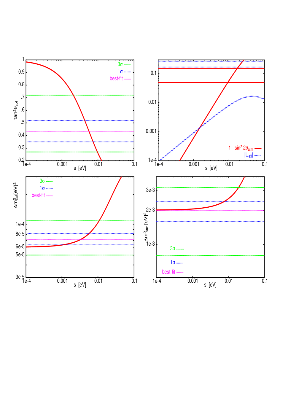
Figure 1: Neutrino mixing parameters as a function of $s$ in case of $CP$ conservation.

In Fig. 1 we show the neutrino mixing parameters as a function of $s$ obtained with the Dirac mass matrix $m_{D}$ from Eq. (19), where for simplicity we set the parameters $a=b=c=d=1$. For the eigenvalues of $m_{L}$ we choose $m_{3}^{0}=0.045$ eV, $m_{2}^{0}=0.008$ eV and $m_{1}^{0}=0.002$ eV. Indicated are the best–fit points as well as the 1 and 3$\sigma$ ranges of the oscillation parameters. With Eqs. (22) and (23) one finds that for, e.g., $s=0.005$ eV the results are $\mbox{$\Delta m^{2}_{\rm A}$}\simeq 2.2\cdot 10^{-3}$ eV², $\mbox{$\Delta m^{2}_{\odot}$}\simeq 8.1\cdot 10^{-5}$ eV², $\tan^{2}\theta_{12}\simeq 0.48$, $1-\sin^{2}2\theta_{23}\simeq 0.015$ and $|U_{e3}|\simeq 0.0044$. Good agreement between these numbers and the plots is found. From the figure it is seen that values of $s$ of a few times $10^{-3}$ eV reproduce the observed deviation from maximal solar neutrino mixing, while predicting small $U_{e3}$ of few times $10^{-3}$ and $1-\sin^{2}2\theta_{23}$ around few times $10^{-2}$. For values of $s\mathrel{\hbox to0.0pt{\raise 2.20013pt\hbox{$>$}\hss}{\lower 2.20013pt\hbox{$\sim$}}}0.01$ eV the parameters except for $|U_{e3}|$ leave their experimentally allowed ranges.

Unfortunately, the implied value of $|U_{e3}|$ is too small to be measured in the next future. Values of this parameter below 0.01 are probably only accessible by a neutrino factory [27]. The implied values of $1-\sin^{2}2\theta_{23}\sim 0.01$, however, could be testable by next generation long–baseline experiments such as JHF–SK [28] or NuMI off–axis [29], all of which claim a sensitivity of $\sigma(\sin^{2}2\theta_{23})\simeq 0.01$.

3.2 Generating $\Delta m^{2}_{\odot}$

It is obvious from Eqs. (7) and (8) that for $A=0$ one would start with vanishing $\Delta m^{2}_{\odot}$. Then, after adding the conventional see–saw term $s$, the induced mass squared difference reads (see Eq. (22)):

$$\mbox{$\Delta m^{2}_{\odot}$}\simeq s~{}\sqrt{2B^{2}+\frac{s^{2}}{16}}\simeq\frac{s^{2}}{4}\frac{1+\tan^{2}\theta_{12}}{1-\tan^{2}\theta_{12}}~{},$$ (26)

i.e., the small conventional see–saw contribution can not only describe the deviation from maximal solar neutrino mixing but also induce non–zero $\mbox{$\Delta m^{2}_{\odot}$}\ll\mbox{$\Delta m^{2}_{\rm A}$}$. Inserting the best–fit points of $\mbox{$\Delta m^{2}_{\odot}$}=7.17\cdot 10^{-5}$ eV² and $\tan^{2}\theta_{12}=0.43$ [14] in the last equation yields that $s\simeq 0.01$ eV, i.e., a value a bit larger than in the $A\neq 0$ case. Consequently, both $U_{e3}$ and $1-\sin^{2}2\theta_{23}$ will also be somewhat larger. For instance, from Eq. (25) one can get

$$\sqrt{\mbox{$\Delta m^{2}_{\rm A}$}}\simeq s~{}\frac{\sin 2\theta_{23}}{\sqrt{1-\sin^{2}2\theta_{23}}}~{},$$ (27)

which for $\mbox{$\Delta m^{2}_{\rm A}$}=2\cdot 10^{-3}$ eV² and $s\simeq 0.01$ eV yields $1-\sin^{2}2\theta_{23}\simeq 0.05$. Another way to distinguish the cases $A=0$ and $A\neq 0$ would be to note that $A=\mbox{$\langle m\rangle$}$ and then to prove that $\mbox{$\langle m\rangle$}=0$. This, however, will in practice not be possible.

It is now for $A=0$ also possible to give a concise formula for the phenomenologically interesting ratio of the solar and atmospheric mass squared ratios. Using Eq. (22) one finds

$$\frac{\mbox{$\Delta m^{2}_{\odot}$}}{\mbox{$\Delta m^{2}_{\rm A}$}}\simeq\frac{1}{4}\,\frac{1+\tan^{2}\theta_{12}}{1-\tan^{2}\theta_{12}}\,\frac{1-\sin^{2}2\theta_{23}}{\sin^{2}2\theta_{23}}~{}.$$ (28)

The ratio of the mass squared differences is thus linked to a small deviation of $\theta_{23}$ from $\pi/4$.

Note that from Eqs. (22) and (26) it holds that $R\propto s^{2}$. Remembering from above that the parameter describing the deviations from bimaximal mixing is $\lambda\propto s$ we see that $R\propto\lambda^{2}$. Therefore, the framework described here gives an explanation for the fact that the ratio of $\Delta m^{2}_{\odot}$ and $\Delta m^{2}_{\rm A}$ is numerically linked [7] to the observed deviation from maximal solar neutrino mixing.

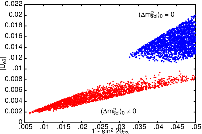
Figure 2: Scatter plot of the observables $|U_{e3}|$ and $1-\sin^{2}2\theta_{23}$ obtained for the cases $A=0$ and $A\neq 0$ in case of $CP$ conservation.

In Fig. 2 we show a scatter plot of the observables $|U_{e3}|$ and $1-\sin^{2}2\theta_{23}$ obtained for the cases $A=0$ and $A\neq 0$. To produce the plots, $m_{i}^{0}$ was varied according to a hierarchical spectrum and $s$ was required to be smaller than $m_{3}^{0}$. The oscillation parameters were required to lie inside their 1$\sigma$ ranges. Both parameters are seen to prefer larger values when $\Delta m^{2}_{\odot}$ is induced by the type I see–saw term. In this particular example and if $A\neq 0$ ($A=0$) lower limits on $U_{e3}$ of 0.002 (0.011) can be set. For $1-\sin^{2}2\theta_{23}$ the lower limits is 0.006 (0.033). Though being slightly larger, the indicated values of $|U_{e3}|\mathrel{\hbox to0.0pt{\raise 2.20013pt\hbox{$>$}\hss}{\lower 2.20013pt\hbox{$\sim$}}}0.01$ mean that they are still too small for next generation experiments but testable by the JHF–HK setup [28].

4 $CP$ violation

4.1 General considerations

In type II see–saw models the number of independent phases is obviously larger than in type I. It has been shown [12, 31] that the Lagrangian (10) contains (for 3 left– and 3 right–handed neutrinos) 12 independent phases. Let us write the relevant matrices $f$ and $m_{D}$ in the following way:

$$f=U_{f}^{\ast}~{}f^{\rm diag}~{}U_{f}^{\dagger}~{}\mbox{ and }~{}m_{D}=U_{1}^{\dagger}~{}m_{D}^{\rm diag}~{}U_{2}~{}.$$ (29)

The eigenvalues of $m_{L}$ are given by $m_{i}^{0}=v_{L}~{}f^{\rm diag}_{i}$. Unitary matrices such as $U_{f}$ can always be written as [32]

$$U_{f}=e^{i\phi}~{}P_{f}~{}\tilde{U}_{f}~{}Q_{f}~{},$$ (30)

where $P_{f}={\rm diag}(1,e^{i\alpha},e^{i\beta})$ and $Q_{f}={\rm diag}(1,e^{i\rho},e^{i\sigma})$ are diagonal matrices containing 2 phases each and $\tilde{U}_{f}$ is a unitary matrix parametrized in analogy to the CKM matrix, i.e., it is defined by 3 angles and 1 phase. Analogous definitions hold for $U_{1}$ and $U_{2}$. Using Eq. (12) one finds after some simple steps:

$$\begin{array}[]{c}m_{\nu}=v_{L}~{}\left(e^{-2i\phi}P_{f}^{\dagger}~{}\tilde{U}_{f}^{\ast}~{}Q_{f}^{\dagger}~{}f^{\rm diag}~{}Q_{f}^{\dagger}~{}\tilde{U}_{f}^{\dagger}~{}P_{f}^{\dagger}-\right.\\[5.69046pt] \left.\frac{\displaystyle e^{i(2\phi_{2}-2\phi_{1}+\phi)}}{\displaystyle\gamma\,v^{2}}~{}Q_{2}~{}\tilde{U}_{2}^{T}~{}\tilde{P}_{2}~{}m_{D}^{\rm diag}~{}\tilde{U}_{1}^{\ast}~{}Q_{1}^{\dagger}~{}P_{f}~{}\tilde{U}_{f}~{}Q_{f}^{2}~{}(f^{\rm diag})^{-1}~{}\tilde{U}_{f}^{T}~{}P_{f}~{}Q_{1}^{\dagger}~{}\tilde{U}_{1}^{\dagger}~{}m_{D}^{\rm diag}~{}\tilde{P}_{2}~{}\tilde{U}_{2}~{}Q_{2}\right),\end{array}$$ (31)

where $\tilde{P}_{2}=P_{1}^{\dagger}~{}P_{2}$ was defined. In the neutrino mass term $\nu^{T}\,m_{\nu}\,\nu$ one can choose now new fields $\nu\rightarrow\nu^{\prime}\equiv e^{-i\phi}~{}P_{f}^{\dagger}\,\nu$, and make the same transformation for the charged leptons. This will alter the above equation to

$$\begin{array}[]{c}m_{\nu}=v_{L}~{}\left(\tilde{U}_{f}^{\ast}~{}Q_{f}^{\dagger}~{}f^{\rm diag}~{}Q_{f}^{\dagger}~{}\tilde{U}_{f}^{\dagger}-\right.\\[5.69046pt] \left.\frac{\displaystyle e^{2i(\phi_{2}-\phi_{1}+\phi)}}{\displaystyle\gamma\,v^{2}}~{}P_{f}~{}Q_{2}~{}\tilde{U}_{2}^{T}~{}\tilde{P}_{2}~{}m_{D}^{\rm diag}~{}\tilde{U}_{1}^{\ast}~{}Q_{1}^{\dagger}~{}P_{f}~{}\tilde{U}_{f}~{}Q_{f}^{2}~{}(f^{\rm diag})^{-1}~{}\tilde{U}_{f}^{T}~{}P_{f}~{}Q_{1}^{\dagger}~{}\tilde{U}_{1}^{\dagger}~{}m_{D}^{\rm diag}~{}\tilde{P}_{2}~{}\tilde{U}_{2}~{}Q_{2}~{}P_{f}\right)\end{array}$$ (32)

Thus, at this point, $m_{\nu}^{II}$ contributes with 3 phases (2 in $Q_{f}$ and 1 in $\tilde{U}_{f}$) to $m_{\nu}$ and the conventional type I term with an additional 9 (1 common, 2 in $P_{f}~{}Q_{2}$, 1 each in $\tilde{U}_{1,2}$, 2 each in $Q_{1}$ and $\tilde{P}_{2}$), corresponding to the mentioned result of 12 independent $CP$ restrictions. As two known limits, consider the cases when the second or the first term is absent. If the second term vanishes, we have nothing more to absorb and hence we end up with the well–known result of three physical phases for a symmetric $3\times 3$ neutrino mass matrix. If only the conventional see–saw term is present and in addition the right–handed Majorana neutrino mass matrix is real and diagonal (as it is possible to go into this basis), we have $\tilde{U}_{f}=P_{f}=Q_{f}=\mathbbm{1}$. Then, from the second term in Eq. (32) the 2 phases in $Q_{2}$ and the common phase $2(\phi_{2}-\phi_{1}+\phi)$ can be absorbed in the charged lepton fields and there are in total 6 phases, which will combine in a complicated manner to the three measurable ones. Six is the well–known number of independent $CP$ restrictions in general three neutrino type I see–saw models [32, 33].

4.2 Our special case

Our requirement of $m_{L}$ being bimaximal will remove the phase from $\tilde{U}_{f}$ and the presence of 3 zeros (or very small entries) in $m_{D}$ will render 3 more phases unphysical. Let us define

$$m_{D}\simeq m\left(\begin{array}[]{ccc}0&a\,e^{i\varphi_{1}}\,\epsilon_{D}^{3}&0\\[8.5359pt] b\,e^{i\varphi_{2}}\,\epsilon_{D}^{3}&e^{i\varphi_{3}}\,\epsilon_{D}^{2}&c\,e^{i\varphi_{4}}\,\epsilon_{D}^{2}\\[8.5359pt] 0&d\,e^{i\varphi_{5}}\,\epsilon_{D}^{2}&e^{i\varphi_{6}}\end{array}\right)~{}.$$ (33)

Then, the 33 entry of the conventional see–saw term reads

$$\begin{array}[]{c}s=(m_{D}^{T}\,M_{R}^{-1}\,m_{D})_{33}\simeq v_{L}^{2}~{}\frac{\displaystyle m^{2}}{\displaystyle 4\,\gamma\,v^{2}}\,e^{2i(\beta+\phi+\varphi_{6})}\left(\frac{\displaystyle 1}{\displaystyle m_{1}^{0}}+\frac{\displaystyle e^{2i\rho}}{\displaystyle m_{2}^{0}}+\frac{\displaystyle 2\,e^{2i\sigma}}{\displaystyle m_{3}^{0}}\right)\\[5.69046pt] \simeq v_{L}^{2}~{}\frac{\displaystyle m^{2}}{\displaystyle 4\,\gamma\,v^{2}}\frac{\displaystyle e^{2i(\beta+\phi+\varphi_{6})}}{\displaystyle m_{1}^{0}}~{}.\end{array}$$ (34)

All other entries of $m_{D}^{T}\,M_{R}^{-1}\,m_{D}$ are suppressed by terms of at least order $\epsilon_{D}^{2}$. With the above $s$ the neutrino mass matrix is

$$m_{\nu}\simeq v_{L}e^{-2i\phi}~{}P_{f}^{\dagger}~{}\tilde{U}_{f}^{\ast}~{}Q_{f}^{\dagger}~{}f^{\rm diag}~{}Q_{f}^{\dagger}~{}\tilde{U}_{f}^{\dagger}~{}P_{f}^{\dagger}-|s|\,e^{2i(\beta+\phi+\varphi_{6})}~{}{\rm diag}(0,0,1)~{}.$$ (35)

In the neutrino mass term $\nu^{T}\,m_{\nu}\,\nu$ one can choose now as before new fields according to $\nu\rightarrow\nu^{\prime}\equiv e^{-i\phi}~{}P_{f}^{\dagger}\,\nu$, and make the same transformation for the charged leptons. This will alter the above equation to

$$m_{\nu}\simeq v_{L}\,\tilde{U}_{f}^{\ast}~{}Q_{f}^{\dagger}~{}f^{\rm diag}~{}Q_{f}^{\dagger}~{}\tilde{U}_{f}^{\dagger}-|s|\,e^{i\delta_{I}}~{}{\rm diag}(0,0,1)~{},$$ (36)

where we have defined

$$\delta_{I}\equiv 2(\varphi_{6}+2(\beta+\phi))~{}.$$ (37)

Recall that due to its bimaximality $\tilde{U}_{f}$ is real. The difference between the $CP$ violating and conserving cases is the presence of two “Majorana–like” phases $\rho,\sigma$ in $Q_{f}$ for the eigenvalues of $m_{L}$ and the subtraction of a small term $s$, which in general is now complex. The phase of $s$ is a combination of one phase in $m_{D}$ and two in $m_{L}$. Note that in general the parameter $\gamma$ appearing in $s$ could also be complex and therefore could also contribute to the relative phase between the two terms in Eq. (36).

It is interesting to consider $CP$ violating observables in the lepton sector. The rephasing invariant $J_{CP}$ [34], which governs the magnitude of $CP$ violating effects in neutrino oscillations [35], can be written in terms of the neutrino mass matrix as [36]

$$J_{CP}=-\frac{{\rm Im}(h_{12}\,h_{23}\,h_{31})}{\Delta m^{2}_{21}\,\Delta m^{2}_{31}\,\Delta m^{2}_{32}}~{},\mbox{ where }h=m_{\nu}m_{\nu}^{\dagger}~{}.$$ (38)

In case of $m_{2}^{0}\neq m_{1}^{0}$, i.e., $\Delta m^{2}_{\odot}$ not generated by the conventional see–saw term, one finds from Eq. (36) that for our chosen set of parameters the leading term is

$$J_{CP}\simeq\frac{(m_{2}^{0})^{2}\,(m_{3}^{0})^{2}\,s}{16\,(\mbox{$\Delta m^{2}_{\rm A}$})^{2}\,\mbox{$\Delta m^{2}_{\odot}$}}\left(m_{1}^{0}\,\sin(\delta_{I}+2\rho)-m_{2}^{0}\,\sin\delta_{I}\right)\simeq\frac{-(m_{2}^{0})^{3}\,(m_{3}^{0})^{2}\,s}{16\,(\mbox{$\Delta m^{2}_{\rm A}$})^{2}\,\mbox{$\Delta m^{2}_{\odot}$}}\sin\delta_{I}~{},$$ (39)

which, as it should, vanishes for $s=0$ because this situation would correspond to exact bimaximal neutrino mixing. The order of magnitude is for $m_{3}^{0}=0.045$ eV, $m_{2}^{0}=0.008$ eV and $m_{1}^{0}=0.002$ eV and the best–fit values of the $\Delta m^{2}$ given by $|J_{CP}|^{\rm max}\simeq 10^{-3}$. Recall that in terms of neutrino mixing angles,

$$J_{CP}=\frac{1}{8}\sin 2\theta_{12}\,\sin 2\theta_{23}\,\sin 2\theta_{13}\,\cos\theta_{13}\,\sin\delta\simeq\frac{1}{4}\sin 2\theta_{12}\,|U_{e3}|\,\sin\delta\sim\frac{|U_{e3}|}{4}\,\sin\delta~{}.$$ (40)

We conclude that $|U_{e3}|$ is of order $10^{-3}\ldots 10^{-2}$. Note that the $ee$ element of the neutrino mass matrix, which is measurable in neutrinoless double beta decay, is given by

$$\mbox{$\langle m\rangle$}=\frac{1}{2}\left(m_{1}^{0}+e^{-2i\rho}m_{2}^{0}\right)~{}.$$ (41)

Therefore, in this particular case the $CP$ violation in neutrino oscillation as governed by $J_{CP}$, which depends only very weakly on $\rho$, is decoupled from the parameter which is responsible for cancellations in the effective mass governing neutrinoless double beta decay.

Now let us consider the case when $\Delta m^{2}_{\odot}$ is induced by the conventional see–saw term. From Eq. (34) one finds that for $m_{1}^{0}=m_{2}^{0}$ and $m_{3}^{0}\gg m_{2}^{0}$:

$$s^{\prime}\simeq v_{L}^{2}~{}\frac{\displaystyle m^{2}}{\displaystyle 2\,\gamma\,v^{2}}\,\frac{\cos\rho}{m_{2}^{0}}\,e^{i(\rho+2(\beta+\phi+\varphi_{6}))}~{},$$ (42)

i.e., a different phase than in Eq. (37) is present. The leading term in $J_{CP}$ will for $m_{3}^{0}\gg m_{2}^{0}$ be proportional to

$$J_{CP}\propto|s^{\prime}|\left(m_{3}^{0}\,\cos(\delta_{I}+2\rho)-|s^{\prime}|\,\cos(\rho-2\sigma)\right)\,\sin\rho~{}.$$ (43)

Since in this case (see Eq. (41)) we have $\mbox{$\langle m\rangle$}=m_{2}^{0}\,\cos\rho$, we find a direct connection between the effective mass in neutrinoless double beta decay and $J_{CP}$.

Regardless if $(\mbox{$\Delta m^{2}_{\odot}$})^{0}=0$ or $(\mbox{$\Delta m^{2}_{\odot}$})^{0}\neq 0$, the entries $A=(m_{1}^{0}+e^{-2i\rho}m_{2}^{0})/2$ and $B=(m_{1}^{0}-e^{-2i\rho}m_{2}^{0})/\sqrt{8}$ should be of the same order to reproduce bi–large neutrino mixing. This implies that $\rho\sim\pi/4$, which is confirmed by a numerical analysis. Also for the $CP$ violating case under consideration, $1-\sin^{2}2\theta_{23}$ and $|U_{e3}|$ will be significantly larger when $(\mbox{$\Delta m^{2}_{\odot}$})^{0}=0$. Consequently, also $|J_{CP}|$ will be larger. Let us choose for a numerical analysis again the values $m_{3}^{0}=0.045$ eV, $m_{2}^{0}=0.008$ eV and $m_{1}^{0}=0.002$ eV or $m_{2}^{0}=m_{1}^{0}=0.008$ eV when $\Delta m^{2}_{\odot}$ is to be generated by $m_{\nu}^{I}$. One will observe that for $(\mbox{$\Delta m^{2}_{\odot}$})^{0}\neq 0$ ($(\mbox{$\Delta m^{2}_{\odot}$})^{0}=0$) $|s|\mathrel{\hbox to0.0pt{\raise 2.20013pt\hbox{$<$}\hss}{\lower 2.20013pt\hbox{$\sim$}}}0.01$ eV ($|s^{\prime}|\mathrel{\hbox to0.0pt{\raise 2.20013pt\hbox{$>$}\hss}{\lower 2.20013pt\hbox{$\sim$}}}0.01$ eV) is the preferred value in order to reproduce the neutrino mixing data. Choosing for definiteness $|s|=0.007$ eV and $|s^{\prime}|/\cos\rho=0.015$ eV, respectively, we can analyze the requisite values of the other parameters.

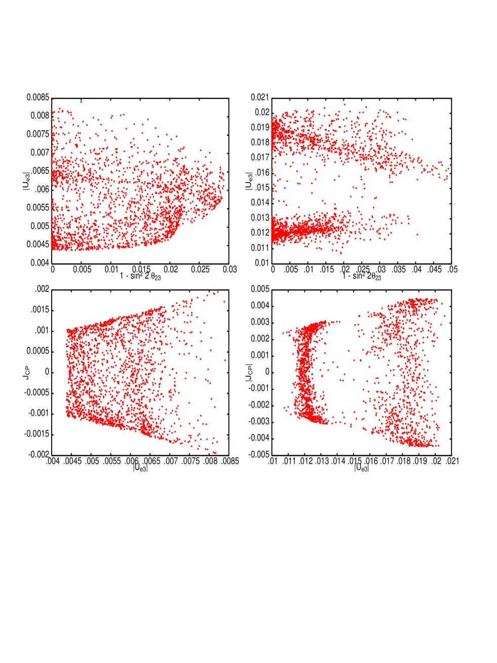
Figure 3: Scatter plots of neutrino mixing parameters $1-\sin^{2}2\theta_{23}$ against $|U_{e3}|$ and $|U_{e3}|$ against $J_{CP}$ when $(\mbox{$\Delta m^{2}_{\odot}$})^{0}\neq 0$ (left column) and $(\mbox{$\Delta m^{2}_{\odot}$})^{0}=0$ (right column).

In Fig. 3 we show the results for some important quantities, namely $1-\sin^{2}2\theta_{23}$ against $|U_{e3}|$ and $|U_{e3}|$ against $J_{CP}$. As mentioned before, also in the $CP$ conserving case the values of $1-\sin^{2}2\theta_{23}$ and $|U_{e3}|$ can be significantly larger than $(\mbox{$\Delta m^{2}_{\odot}$})^{0}=0$. Note, however, that now in case of $CP$ violation atmospheric neutrino mixing can be maximal. Non–zero $U_{e3}$ is however always guaranteed.

4.3 Leptogenesis

Leptogenesis [37] in the framework of type II see–saw mechanism has so far not been discussed in as many details as the type I case (see, e.g., [38] and references therein). The presence of the Higgs triplet $\Delta_{L}$ implies the existence of novel decay processes capable of producing a decay asymmetry. In the usual type I see–saw approach the decay $N_{i}\rightarrow\Phi\,\ell$, where $N_{i}$ is one of the heavy Majorana neutrinos, $\Phi$ the Higgs doublet and $\ell$ a lepton, receives 1–loop self–energy and vertex corrections, where for the latter a virtual heavy Majorana neutrino $N_{j}$ is exchanged. The decay asymmetry stemming from these two diagrams will be called $\varepsilon_{1}^{N}$. When a triplet is present, it also will be exchanged in the vertex correction to the decay $N_{1}\rightarrow\Phi\,\ell$ [39, 40], giving rise to a decay asymmetry $\varepsilon_{1}^{\Delta}$. Furthermore, the decay $\Delta_{L}\rightarrow\ell\,\ell$ is possible, which will receive 1–loop vertex corrections via virtual Majorana neutrino exchange [39, 40]. If the triplet mass $M_{\Delta}$ is much larger than the Majorana neutrino masses, the baryon asymmetry is produced via the decay of the Majorana neutrinos. Let us focus on this situation, since typically for the mass of the triplet $m_{\Delta_{L}}\sim v_{R}$ holds, which is larger than the mass of the lightest of the heavy Majorana neutrinos. The decay asymmetries for the heavy Majorana neutrino decay read

$$\begin{array}[]{c}\varepsilon_{1}^{N}=\frac{\displaystyle 1}{\displaystyle 8\pi\,v^{2}}\,\frac{\displaystyle 1}{\displaystyle(\tilde{m}_{D}\tilde{m}_{D}^{\dagger})_{11}}\,\sum\limits_{j=2,3}\,{\rm Im}\left\{(\tilde{m}_{D}\tilde{m}_{D}^{\dagger})^{2}_{1j}\right\}\,f_{N}\left(\frac{\displaystyle M_{j}^{2}}{\displaystyle M_{1}^{2}}\right)~{},\\[8.5359pt] \varepsilon_{1}^{\Delta}=\frac{\displaystyle-3\,v_{L}}{\displaystyle 8\pi\,v^{2}}\,\frac{\displaystyle 1}{\displaystyle(\tilde{m}_{D}\tilde{m}_{D}^{\dagger})_{11}}\,\frac{\displaystyle M_{\Delta}^{2}}{\displaystyle M_{1}}\,{\rm Im}\left\{(\tilde{m}_{D}f^{\ast}\,\tilde{m}_{D}^{T})_{11}\right\}\,f_{\Delta}\left(\frac{\displaystyle M_{\Delta}^{2}}{\displaystyle M_{1}^{2}}\right)~{},\end{array}$$ (44)

where $\varepsilon_{1}^{\Delta}$ has been calculated recently [40, 41]. We wrote the expressions in terms of $\tilde{m}_{D}=U_{f}^{\dagger}\,m_{D}$, because we have to work in the basis in which the heavy Majorana neutrinos are diagonal. The functions $f_{N}$ and $f_{\Delta}$ are given by

$$\begin{array}[]{c}f_{N}(x)=\sqrt{x}\left(1-(1+x)\log(1+1/x)+\frac{\displaystyle 1}{\displaystyle 1-x}\right)\simeq\frac{\displaystyle-3}{\displaystyle 2\sqrt{x}}~{},\\[8.5359pt] f_{\Delta}(x)=1-x\log(1+1/x)\simeq\frac{\displaystyle 1}{\displaystyle 2x}~{},\end{array}$$ (45)

where the limits for $x\gg 1$ were given. Using these approximations, the asymmetries can be written as

$$\begin{array}[]{c}\varepsilon_{1}^{N}=\frac{\displaystyle 3}{\displaystyle 16\pi\,v^{2}}\,\frac{\displaystyle M_{1}}{\displaystyle(\tilde{m}_{D}\tilde{m}_{D}^{\dagger})_{11}}\,{\rm Im}\left\{(\tilde{m}_{D}(m_{\nu}^{I})^{\ast}\,\tilde{m}_{D}^{T})_{11}\right\}~{},\\[8.5359pt] \varepsilon_{1}^{\Delta}=\frac{\displaystyle 3}{\displaystyle 16\pi\,v^{2}}\,\frac{\displaystyle M_{1}}{\displaystyle(\tilde{m}_{D}\tilde{m}_{D}^{\dagger})_{11}}\,{\rm Im}\left\{(\tilde{m}_{D}(m_{\nu}^{II})^{\ast}\,\tilde{m}_{D}^{T})_{11}\right\}~{}.\end{array}$$ (46)

As first observed in [40], if $m_{\nu}^{I}$ ($m_{\nu}^{II}$) dominates in $m_{\nu}$, one would expect $\varepsilon_{1}^{N}$ ($\varepsilon_{1}^{\Delta}$) to dominate the decay asymmetry. To check this assumption in our scenario, let us write $m_{D}\simeq m\,e^{i\varphi_{6}}\,{\rm diag}(0,0,1)$ and take $U_{f}$ and $f$ from Eq. (29) and (30) in order to calculate $m_{\nu}^{II}=v_{L}\,U_{f}^{\ast}~{}f^{\rm diag}~{}U_{f}^{\dagger}$. For $m_{\nu}^{I}$ we have to calculate $M_{R}^{-1}$, which is given by $v_{L}/v_{R}\,m_{L}^{-1}=U_{f}~{}(v_{R}~{}f^{\rm diag})^{-1}~{}U_{f}^{T}$. The result for $m_{3}^{0}\gg m_{1,2}^{0}$ and $m_{2}^{0}\neq m_{1}^{0}$ is

$$\begin{array}[]{c}\varepsilon_{1}^{N}\simeq\frac{\displaystyle-3}{\displaystyle 64\,\pi}\,\frac{\displaystyle m^{2}}{\displaystyle v^{2}}\,\frac{\displaystyle v_{L}}{\displaystyle v_{R}}\,\frac{\displaystyle M_{1}}{\displaystyle m_{1}^{0}}\,\sin 4\varphi_{6}~{},\\[8.5359pt] \varepsilon_{1}^{\Delta}\simeq\frac{\displaystyle-3}{\displaystyle 32\,\pi\,v^{2}}\,M_{1}~{}m_{3}^{0}~{}\sin 2(2\beta+2\phi-\varphi_{6}+\sigma)~{},\end{array}$$ (47)

We can clarify the situation significantly when we note that $v_{L}/v_{R}=v_{L}^{2}/(\gamma\,v^{2})$ and by glancing at Eq. (34), where $s$ is defined. Furthermore, we can express $m_{3}^{0}$ through $D$, the heaviest entry in $m_{\nu}^{\rm bimax}$ from Eq. (7). Then the above forms of the decay asymmetries can be rewritten as

$$\begin{array}[]{c}\varepsilon_{1}^{N}\simeq\frac{\displaystyle-3M_{1}}{\displaystyle 16\pi\,v^{2}}\,|s|\,\sin 4\varphi_{6}~{},\\[8.5359pt] \varepsilon_{1}^{\Delta}\simeq\frac{\displaystyle-3\,M_{1}}{\displaystyle 16\pi\,v^{2}}\,|D|\,\sin 2(2\beta+2\phi-\varphi_{6}+\sigma)~{}.\end{array}$$ (48)

As is should, the asymmetry $\varepsilon_{1}^{N}$ proportional to $m_{\nu}^{I}$ vanishes for $s=0$, i.e., when there is no conventional type I see–saw term. It is seen that the contribution to the decay asymmetry stemming from the exchange of virtual Majorana neutrinos is suppressed in comparison to virtual triplet exchange by a typical factor of (ignoring phases)

$$\left|\frac{\varepsilon_{1}^{N}}{\varepsilon_{1}^{\Delta}}\right|\simeq\left|\frac{s}{D}\right|~{}.$$ (49)

This is easily interpreted as the ratio of the the maximal entries in $m_{\nu}^{II}$ and $m_{\nu}^{I}$, respectively. This conclusion holds also when we use the full Dirac mass matrix Eq. (33). Since there are here (and in general) unmeasurable combinations of phases involved in $\varepsilon_{1}^{\Delta}$, however, it is possible that $\varepsilon_{1}^{N}$ dominates the baryon asymmetry though the main contribution to $m_{\nu}$ stems from $m_{\nu}^{II}$. In Refs. [24, 20] a detailed bottom–up analysis of such scenarios can be found.

Not surprisingly, without assuming any more simplifications of the mass matrices, the high energy $CP$ violation as required for leptogenesis in the decay asymmetries Eqs. (47) decouples from the $CP$ violation as measurable at low energy in $\langle m\rangle$ or $J_{CP}$ as given in (39). The same is true for the connection of low and high energy $CP$ violation in general type I see–saw models [33, 32].

Note that within our framework the upper limit on the decay asymmetry is given by

$$|\varepsilon_{1}^{\rm max}|\simeq\frac{3}{16\pi}\,\frac{M_{1}}{v^{2}}(D+|s|)\simeq\frac{3}{16\pi}\,\frac{M_{1}}{v^{2}}\,\left(\frac{m_{3}}{2}+\frac{5}{4}|s|\right)\simeq\frac{3}{32\pi}\,\frac{M_{1}}{v^{2}}\,\sqrt{\mbox{$\Delta m^{2}_{\rm A}$}}~{}.$$ (50)

Hence, this upper limit is not much difficult (roughly a factor 2 weaker) from the usual bound in the conventional type I see–saw leptogenesis scenario [42], $|\varepsilon_{1}^{N}|<\frac{3}{16\pi}\,\frac{M_{1}}{v^{2}}\,\sqrt{\mbox{$\Delta m^{2}_{\rm A}$}}$. This latter bound is valid for light neutrinos with normal or inverted mass hierarchy. In these cases, the limits on the decay asymmetry within the type I and type II see–saw mechanism are identical [41]. However, in the type II see–saw scenario, assuming quasi–degenerate light neutrinos with a common mass scale $m_{0}$, a bound of $|\varepsilon_{1}^{\Delta}+\varepsilon_{1}^{N}|<\frac{3}{16\pi}\,\frac{M_{1}}{v^{2}}\,m_{0}$ can be derived [41]. This has to be contrasted with the limit $|\varepsilon_{1}^{N}|\mathrel{\hbox to0.0pt{\raise 2.20013pt\hbox{$<$}\hss}{\lower 2.20013pt\hbox{$\sim$}}}\frac{3}{32\pi}\,\frac{M_{1}}{v^{2}}\,\frac{\Delta m^{2}_{\rm atm}}{m_{0}}$ in case of leptogenesis within the type I see–saw mechanism [42]. Therefore, in case of type II see–saw the upper limit on the decay asymmetry for quasi–degenerate neutrinos is weaker by a factor of $2m_{0}^{2}/\mbox{$\Delta m^{2}_{\rm A}$}$ with respect to the limit in case of the conventional type I see–saw. We remark that quasi–degenerate light neutrinos are more natural to obtain in type II see–saw scenarios.

One can check if the decay asymmetry has the correct order of magnitude to generate a sufficient baryon asymmetry. Let us assume for this purpose that the wash–out processes in our framework yield an efficiency factor for the lepton asymmetry of similar magnitude as in the usual conventional scenarios [38]. Solving the complete set of Boltzmann–equations is beyond the scope of this study. The overall scale of the decay asymmetries can be rewritten as

$$\begin{array}[]{c}\left|\varepsilon_{1}^{N}+\varepsilon_{1}^{\Delta}\right|\mathrel{\hbox to0.0pt{\raise 2.20013pt\hbox{$<$}\hss}{\lower 2.20013pt\hbox{$\sim$}}}10^{-6}\left(\frac{\displaystyle M_{1}}{\displaystyle 10^{10}\,\rm GeV}\right)\,\left(\frac{\displaystyle m_{3}^{0}}{\displaystyle\sqrt{2\cdot 10^{-3}\,\rm eV^{2}}}\right)\\[8.5359pt] \sim 10^{-3}\left(\frac{\displaystyle v_{R}}{\displaystyle 10^{15}\,\rm GeV}\right)^{2}\,\left(\frac{\displaystyle m_{1}^{0}}{\displaystyle 10^{-3}\,\rm eV}\right)\,\left(\frac{\displaystyle m_{3}^{0}}{\displaystyle\sqrt{2\cdot 10^{-3}\,\rm eV^{2}}}\right)~{},\end{array}$$ (51)

where we used that $M_{i}=m_{i}\,v_{R}/v_{L}$ and $v_{R}\,v_{L}\sim v^{2}$. The order of magnitude of the decay asymmetry typically required for succesful leptogenesis is about $10^{-6}$ [38]. Hence, as in the bottom–up analysis of [24] in case of hierarchical light neutrinos and $m_{D}$ being related to the up–quarks, the decay asymmetry is for the “natural” value $v_{R}=10^{15}$ GeV typically too large and requires some suppression by the phases or by somewhat smaller values of $v_{R}$.

5 Summary

The simple toy model presented in this paper serves to underline possible interplay of both terms in the type II see–saw formula. In type II see–saw scenarios it is possible that the conventional see–saw term $m_{D}^{T}M_{R}^{-1}m_{D}$ naturally gives only a small correction $s$ to the dominating triplet term $m_{L}$. It is tempting to assume that the dominating $m_{L}$ corresponds to bimaximal neutrino mixing. Then, as demonstrated in the present article, the small contribution $s$ from the conventional see–saw term can be sufficient to pull solar neutrino mixing away from being maximal. If this mechanism is realized, $|U_{e3}|$ and $1-\sin^{2}2\theta_{23}$ receive corrections from zero of order 0.001 and 0.01, respectively. The presence of $CP$ violation does not change the typical behavior of those observables, except that atmospheric mixing can be allowed to be maximal. If the type I see–saw term is also responsible for generating the solar $\Delta m^{2}$, both $|U_{e3}|$ and $1-\sin^{2}2\theta_{23}$ are significantly larger.

The deviation from maximal solar neutrino mixing is described most conveniently and naturally via $U_{e2}=\sqrt{1/2}~{}(1-\lambda)$ and the other deviations from bimaximal neutrino mixing will be proportional to appropriate powers of $\lambda$ as well. The ratio $R$ of the solar and atmospheric mass squared differences turns out to be of the order $\lambda^{2}$. This apparent coincidence is explained by the framework described in the present paper when one starts with vanishing $\Delta m^{2}_{\odot}$, because it holds that $\lambda\propto s$ and $R\propto s^{2}$.

Since the type II term is consequence of a $SU(2)_{L}$ Higgs triplet term, this triplet can also contribute to the decay asymmetry in leptogenesis scenarios. The decay asymmetry produced by the exchange of virtual triplets is typically larger than the one produced by heavy Majorana exchange by a factor corresponding to the ratio of the maximal entries in $m_{\nu}^{II}$ and $m_{\nu}^{I}$.

Acknowledgments

It is a pleasure to thank Sandhya Choubey for invaluable comments. This work was supported by the EC network HPRN-CT-2000-00152.

References

- [1] F. Vissani, hep-ph/9708483; V. D. Barger, S. Pakvasa, T. J. Weiler and K. Whisnant, Phys. Lett. B 437, 107 (1998); A. J. Baltz, A. S. Goldhaber and M. Goldhaber, Phys. Rev. Lett. 81, 5730 (1998); H. Georgi and S. L. Glashow, Phys. Rev. D 61, 097301 (2000); I. Stancu and D. V. Ahluwalia, Phys. Lett. B 460, 431 (1999).
- [2] S. N. Ahmed et al. [SNO Collaboration], Phys. Rev. Lett. 92, 181301 (2004).
- [3] K. Eguchi et al. [KamLAND Collaboration], Phys. Rev. Lett. 90, 021802 (2003).
- [4] S. T. Petcov, Phys. Lett. B 110, 245 (1982).
- [5] E.g., M. Jezabek and Y. Sumino, Phys. Lett. B 457, 139 (1999); Z. z. Xing, Phys. Rev. D 64, 093013 (2001); T. Ohlsson and G. Seidl, Nucl. Phys. B 643, 247 (2002); C. Giunti and M. Tanimoto, Phys. Rev. D 66, 053013 (2002); Phys. Rev. D 66, 113006 (2002); G. Altarelli, F. Feruglio and I. Masina, Nucl. Phys. B 689, 157 (2004); A. Romanino, hep-ph/0402258.
- [6] S. F. King, JHEP 0209, 011 (2002).
- [7] W. Rodejohann, Phys. Rev. D 69, 033005 (2004).
- [8] P. H. Frampton, S. T. Petcov and W. Rodejohann, Nucl. Phys. B 687, 31 (2004).
- [9] S. Antusch et al., Phys. Lett. B 544, 1 (2002); T. Miura, T. Shindou and E. Takasugi, Phys. Rev. D 68, 093009 (2003); B. Stech and Z. Tavartkiladze, hep-ph/0311161; T. Shindou and E. Takasugi, hep-ph/0402106.
- [10] W. Rodejohann, Eur. Phys. J. C 32, 235 (2004).
- [11] R. Barbieri et al., JHEP 9812, 017 (1998); G. Altarelli and F. Feruglio, JHEP 9811, 021 (1998); S. Davidson and S. F. King, Phys. Lett. B 445, 191 (1998); R. N. Mohapatra and S. Nussinov, Phys. Rev. D 60, 013002 (1999); C. H. Albright and S. M. Barr, Phys. Lett. B 461, 218 (1999); Y. Nomura and T. Yanagida, Phys. Rev. D 59, 017303 (1999); A. S. Joshipura and S. D. Rindani, Eur. Phys. J. C 14, 85 (2000); R. N. Mohapatra, A. Perez-Lorenzana and C. A. de Sousa Pires, Phys. Lett. B 474, 355 (2000); A. Aranda, C. D. Carone and P. Meade, Phys. Rev. D 65, 013011 (2002); R. Kitano and Y. Mimura, Phys. Rev. D 63, 016008 (2001); K. S. Babu and S. M. Barr, Phys. Lett. B 525, 289 (2002); H. S. Goh, R. N. Mohapatra and S. P. Ng, Phys. Lett. B 542, 116 (2002). A. de Gouvea, Phys. Rev. D 69, 093007 (2004).
- [12] J. Schechter and J. W. F. Valle, Phys. Rev. D 22, 2227 (1980).
- [13] B. Pontecorvo, Zh. Eksp. Teor. Fiz. 33, 549 (1957) and 34, 247 (1958); Z. Maki, M. Nakagawa and S. Sakata, Prog. Theor. Phys. 28, 870 (1962).
- [14] A. Bandyopadhyay et al., Phys. Lett. B 583, 123 (2004).
- [15] G. L. Fogli et al., Phys. Rev. D 67, 093006 (2003).
- [16] M. Gell–Mann, P. Ramond, and R. Slansky in Supergravity, p. 315, edited by F. Nieuwenhuizen and D. Friedman, North Holland, Amsterdam, 1979; T. Yanagida, Proc. of the Workshop on Unified Theories and the Baryon Number of the Universe, edited by O. Sawada and A. Sugamoto, KEK, Japan 1979; R. N. Mohapatra and G. Senjanovic, Phys. Rev. Lett. 44, 912 (1980).
- [17] G. Lazarides, Q. Shafi and C. Wetterich, Nucl. Phys. B 181, 287 (1981); R. N. Mohapatra and G. Senjanovic, Phys. Rev. D 23, 165 (1981); J. Schechter and J. W. F. Valle, Phys. Rev. D 25, 774 (1982).
- [18] B. Bajc, G. Senjanovic and F. Vissani, Phys. Rev. Lett. 90, 051802 (2003); hep-ph/0402140; H. S. Goh, R. N. Mohapatra and S. P. Ng, Phys. Lett. B 570, 215 (2003); Phys. Rev. D 68, 115008 (2003).
- [19] E. Ma, Phys. Rev. D 69, 011301 (2004).
- [20] A. S. Joshipura, E. A. Paschos and W. Rodejohann, JHEP 0108, 029 (2001); W. Rodejohann, Phys. Lett. B 542, 100 (2002).
- [21] S. Nasri, J. Schechter and S. Moussa, hep-ph/0402176.
- [22] See, e.g., J. A. Casas et al., Nucl. Phys. B 573, 652 (2000); P. H. Chankowski and S. Pokorski, Int. J. Mod. Phys. A 17, 575 (2002); S. Antusch et al., Nucl. Phys. B 674, 401 (2003) and references therein.
- [23] S. Antusch and S. F. King, hep-ph/0402121; for triplet dominated earlier models see, e.g., D. O. Caldwell and R. N. Mohapatra, Phys. Rev. D 48, 3259 (1993); A. Ioannisian and J. W. F. Valle, Phys. Lett. B 332, 93 (1994).
- [24] A. S. Joshipura and E. A. Paschos, hep-ph/9906498; A. S. Joshipura, E. A. Paschos and W. Rodejohann, Nucl. Phys. B 611, 227 (2001).
- [25] O. Cremonesi, Invited talk at the XXth Internat. Conf. on Neutrino Physics and Astrophysics (Neutrino 2002), Munich, Germany, May 25-30, 2002, Nucl. Phys. Proc. Suppl. 118, 287 (2003) (hep-ex/0210007).
- [26] Y. Hayato, talk Presented at International Europhysics Conference on High-Energy Physics (HEP 2003), Aachen, Germany, 17-23 Jul 2003, http://eps2003.physik.rwth-aachen.de/transparencies/07/index.php.
- [27] C. Albright et al., hep-ex/0008064; M. Apollonio et al., hep-ph/0210192.
- [28] Y. Itow et al., hep-ex/0106019.
- [29] D. Ayres et al., hep-ex/0210005.
- [30] P. H. Frampton, S. L. Glashow and D. Marfatia, Phys. Lett. B 536, 79 (2002).
- [31] G. C. Branco, L. Lavoura and M. N. Rebelo, Phys. Lett. B 180, 264 (1986).
- [32] S. Pascoli, S. T. Petcov and W. Rodejohann, Phys. Rev. D 68, 093007 (2003).
- [33] G. C. Branco et al., Nucl. Phys. B 617, 475 (2001).
- [34] C. Jarlskog, Z. Phys. C 29, 491 (1985); Phys. Rev. D 35, 1685 (1987).
- [35] P. I. Krastev and S. T. Petcov, Phys. Lett. B 205, 84 (1988).
- [36] G. C. Branco et al., Phys. Rev. D 67, 073025 (2003).
- [37] M. Fukugita and T. Yanagida, Phys. Lett. B 174, 45 (1986).
- [38] W. Buchmüller, P. Di Bari and M. Plümacher, Nucl. Phys. B 665, 445 (2003); hep-ph/0401240. G. F. Giudice, et al., Nucl. Phys. B 685, 89 (2004).
- [39] P. J. O’Donnell and U. Sarkar, Phys. Rev. D 49, 2118 (1994); G. Lazarides and Q. Shafi, Phys. Rev. D 58, 071702 (1998).
- [40] T. Hambye and G. Senjanovic, Phys. Lett. B 582, 73 (2004).
- [41] S. Antusch and S. F. King, hep-ph/0405093.
- [42] S. Davidson and A. Ibarra, Phys. Lett. B 535, 25 (2002).