Branching ratios of $B^{+}\to D^{(*)+}K^{(*)0}$ decays in perturbative QCD approach

Abstract

We study the rare decays $B^{+}\to D^{(*)+}K^{(*)0}$, which can occur only via annihilation type diagrams in the standard model. We calculate all of the four modes, $B\to PP,~{}VP,~{}PV,~{}VV$, in the framework of perturbative QCD approach and give the branching ratios of the order about $10^{-6}$.

I Introduction

More and more data of $B$ decays are being collected at the two $B$ factories, Belle and BaBar. The original approach to non-leptonic $B$ decays based on the factorization approach (FA) [1], which succeeded in calculating the branching ratios of many decays [2]. FA is a simple method, by which non-factorizable and annihilation contributions are neglected. Although calculations are easy in FA, it suffers the problems of scale, infrared-cutoff and gauge dependence [3]. Especially it is difficult to explain some observed branching ratios of $B$ decays, such as $B\to J/\psi K^{(*)}$ [4]. To improve the theoretical application [5] and understand why the simple FA works so well [6, 7], some methods have been brought forward and developed. One of them is the perturbative QCD (PQCD) approach developed by Brodsky and Lepage [8, 9], under which we can calculate the annihilation diagrams as well as the factorizable and non-factorizable diagrams.

It is consistent to calculate branching ratios of $B$ decays in PQCD approach, as we will explain its framework in the next section. It has been applied in the non-leptonic $B$ decays [6, 7, 10, 11] successfully. In the case of $B^{+}\to D^{(*)+}K^{(*)0}$ decays, which is a kind of pure annihilation type decays, the physics picture of PQCD is as follows, shown in Fig. 1. A $W$ boson exchange causes $\bar{b}u\to\bar{s}c$, and the $\bar{d}d$ quarks are produced from a gluon. In the rest frame of the $B$ meson, the $d$ and $\bar{d}$ quarks in the $D^{(*)+}K^{(*)0}$ mesons each has momentum $\cal{O}$$(M_{B}/4)$, so the gluon producing them has $q^{2}\sim\cal{O}$$(M_{B}^{2}/4)$. It is a hard gluon according to the mass of $B$ meson. So we can perturbatively treat these decays and use PQCD approach like other pure annihilation type $B$ decays [12] .

In the next section, we explain the framework of PQCD briefly. In section 3, we give the analytic formulae for the decays $B^{+}\to D^{(*)+}K^{(*)0}$. In section 4, we show the numerical results and theoretical errors of the four modes respectively. Finally, we draw a conclusion in section 5.

II Framework

The PQCD approach divides the process into hard components, which are treated by perturbative theory, and non-perturbative components, which are put into the hadron wave function. The hadron wave function can be extracted from experimental data or calculated by QCD sum rules method. The decay amplitude can be conceptually written as the convolution

$$\mbox{Amplitude}\sim\int\!\!d^{4}k_{1}d^{4}k_{2}d^{4}k_{3}\ \mathrm{Tr}\bigl{[}C(t)\Phi_{B}(k_{1})\Phi_{D_{s}^{*}}(k_{2})\Phi_{K}(k_{3})H(k_{1},k_{2},k_{3},t)\bigr{]},$$ (1)

where $k_{i}$’s are momenta of light quarks included in each meson, and $\mathrm{Tr}$ denotes the trace over Dirac and color indices. The hard components comprise hard part ($H$) and harder dynamics ($C$). $H(t)$ describes the four quark operator and the spectator quark connected by a hard gluon. It can be perturbatively calculated, since it includes the hard dynamics characterized by the scale $t$, where $t\sim\mathcal{O}$ $(M_{B}/2)$ for $B^{+}\to D^{(*)+}K^{(*)0}$ decays, and the hard gluon’s $q^{2}$ is of the order $t^{2}$. $C(t)$ is the Wilson coefficient which results from the radiative corrections at short distance. In the above convolution, $C(t)$ includes the harder dynamics at a larger scale than the $M_{B}$ scale and describes the evolution of local four-Fermi operators from $M_{W}$ down to the scale $t$. The wave function $\Phi_{M}$ denotes the non-perturbative components, which is independent of the specific processes and removes the infrared cut off dependence in PQCD approach.

According to the conservation of four-momentum, we can obtain $D^{(*)+}$ and $K^{(*)0}$ meson’s energy and momenta in the rest frame of $B$ meson,

$$E_{1}=M_{B},~{}~{}\left|{\bf P}_{1}\right|=0,$$ (2)

$$E_{2}=\frac{M_{B}}{2}(1+r_{2}^{2}-r_{3}^{2}),~{}~{}E_{3}=\frac{M_{B}}{2}(1-r_{2}^{2}+r_{3}^{2}),$$ (3)

$$\left|{\bf P}_{2}\right|=\left|{\bf P}_{3}\right|=\frac{M_{B}}{2}\sqrt{1-2\,{{r_{2}}}^{2}+{{r_{2}}}^{4}-2\,{{r_{3}}}^{2}-2\,{{r_{2}}}^{2}\,{{r_{3}}}^{2}+{{r_{3}}}^{4}},$$ (4)

where the subscript (1,2,3) denote $B^{+}$, $D^{(*)+}$ and $K^{(*)0}$ meson respectively, and $r_{2}=M_{D^{(*)+}}/M_{B}$, $r_{3}=M_{K^{(*)0}}/M_{B}$. It is convenient to assume that the $D^{*+}$ ($K^{*0}$) meson moves in the plus (minus) $z$ direction carrying the momentum $P_{2}$ ($P_{3}$). The longitudinal polarization vectors of the $D^{*+}$ and $K^{*0}$ are given as

$$\epsilon_{2L}=\frac{1}{2r_{2}}(\sqrt{{\left(1-{{r_{3}}}^{2}\right)}^{2}-2\,{{r_{2}}}^{2}\,\left(1+{{r_{3}}}^{2}\right)+{{r_{2}}}^{4}},0,0,1+{{r_{2}}}^{2}-{{r_{3}}}^{2}),$$ (5)

$$\epsilon_{3L}=\frac{1}{2r_{3}}({\sqrt{{\left(1-{{r_{3}}}^{2}\right)}^{2}-2\,{{r_{2}}}^{2}\,\left(1+{{r_{3}}}^{2}\right)+{{r_{2}}}^{4}}},0,0,-1+{{r_{2}}}^{2}-{{r_{3}}}^{2}),$$ (6)

which satisfy the normalization $\epsilon_{2L}^{2}=\epsilon_{3L}^{2}=-1$ and the orthogonality $\epsilon_{2L}\cdot P_{2}=\epsilon_{3L}\cdot P_{3}=0$. For simplicity, we use the light-cone coordinate to describe the meson’s momenta in the rest frame of $B$ meson. After deducing the analytic formulae of amplitudes, we ignore the terms proportional to $r_{2}^{2}\sim 0.15$ or $r_{3}^{2}\sim 0.04$. Equivalently we ignore the terms proportional to $r^{2}$ in $B^{+}$, $D^{(*)+}$ and $K^{(*)0}$ meson’s momenta and longitudinal polarization vectors. Therefore eqs.(4,6) in the light-cone coordinate are corresponding to

$$P_{1}=\frac{M_{B}}{\sqrt{2}}(1,1,{\bf 0}_{T}),\ \ P_{2}=\frac{M_{B}}{\sqrt{2}}(1-r_{3}^{2},r_{2}^{2},{\bf 0}_{T}),\ \ P_{3}=\frac{M_{B}}{\sqrt{2}}(r_{3}^{2},1-r_{2}^{2},{\bf 0}_{T}),$$ (7)

$$\epsilon_{2L}=\frac{1}{\sqrt{2}r_{2}}(1-r_{3}^{2},-r_{2}^{2},{\bf 0}_{T}),\ \ \epsilon_{3L}=\frac{1}{\sqrt{2}r_{3}}(-r_{3}^{2},1-r_{2}^{2},{\bf 0}_{T}),$$ (8)

respectively. The transverse polarization vectors can be adapted directly as $\epsilon_{2T}=(0,0,{\bf 1}_{T})$, $\epsilon_{3T}=(0,0,{\bf 1}_{T})$. We denote the light (anti-)quark momenta in $B^{+}$, $D^{(*)+}$ and $K^{(*)0}$ mesons as $k_{1}=(x_{1}P_{1}^{+},0,{\bf k}_{1T})$, $k_{2}=(x_{2}P_{2}^{+},0,{\bf k}_{2T})$, and $k_{3}=(0,x_{3}P_{3}^{-},{\bf k}_{3T})$ respectively. Integrating eq. (1) over $k_{1}^{-}$, $k_{2}^{-}$, and $k_{3}^{+}$, we obtain

$$\mbox{Amplitude}\sim\int\!\!dx_{1}dx_{2}dx_{3}b_{1}db_{1}b_{2}db_{2}b_{3}db_{3}$$ (9)

$$\mathrm{Tr}\bigl{[}C(t)\Phi_{B}(x_{1},b_{1})\Phi_{D_{s}}(x_{2},b_{2})\Phi_{K}(x_{3},b_{3})H(x_{i},b_{i},t)S_{t}(x_{i})\,e^{-S(t)}\bigr{]},$$ (10)

where $b_{i}$ is the conjugate space coordinate of $k_{iT}$, and $t$ is the largest energy scale in $H$, as a function in terms of $x_{i}$ and $b_{i}$. The large logarithms $\ln(M_{W}/t)$ resulting from QCD radiative corrections to four quark operators are absorbed into the Wilson coefficients $C(t)$. The inclusion of $k_{T}$ brings in one kind of large logarithms $\ln^{2}(Pb)$ from the overlap of collinear and soft gluon corrections, $P$ denoting the dominant light-cone component of meson momentum. The other kind of large logarithms $\ln(tb)$ derives from the renormalization of the ultraviolet divergences. These two kinds of large logarithms are summed and lead to Sudakov form factor, $e^{-S(t)}$. It suppresses the soft dynamics effectively [13]. The large double logarithms $\ln^{2}x_{i}$ are summed by the threshold resummation [14], and they lead to $S_{t}(x_{i})$ which smears the end-point singularities on $x_{i}$. From the brief analysis above, it can be seen that PQCD is a consistent approach.

III Analytic formulae

A The wave functions

We use the wave functions $\Phi_{M,\alpha\beta}$ decomposed in terms of spin structure. The coming $B$ meson and outgoing $D^{(*)+}$, $K^{(*)0}$ are as follows:

$$\Phi_{B}(x,b)=\frac{i}{\sqrt{2N_{c}}}\left[(\not\!P_{1}\gamma_{5})+M_{B}\gamma_{5}\right]\phi_{B}(x,b),$$ (11)

$$\Phi_{D}(x,b)=\frac{i}{\sqrt{2N_{c}}}\left[\gamma_{5}(\not\!P_{2}+M_{D})\right]\phi_{D}(x,b),$$ (12)

$$\Phi_{D^{*}}(x,b)=\frac{i}{\sqrt{2N_{c}}}\left[\not\!\epsilon(\not\!P_{2}+M_{D^{*}})\right]\phi_{D^{*}}(x,b),$$ (13)

$$\Phi_{K}(x,b)=\frac{i}{\sqrt{2N_{c}}}\Bigl{[}\gamma_{5}\not\!P_{3}\phi_{K}^{A}(x,b)+M_{0K}\gamma_{5}\phi_{K}^{P}(x,b)$$ (14)

$$+M_{0K}\gamma_{5}(\not v\not n-1)\phi_{K}^{T}(x,b)\Bigr{]},$$ (15)

$$\Phi_{K^{*}L}(x,b)=\frac{i}{\sqrt{2N_{c}}}\Bigl{[}M_{K^{*}}\not\!\epsilon_{3L}\phi_{K^{*}}(x,b)+\not\!\epsilon_{3L}\not\!P_{3}\phi_{K^{*}}^{t}(x,b)$$ (16)

$$+M_{K^{*}}I\phi_{K^{*}}^{s}(x,b)\Bigr{]},$$ (17)

$$\Phi_{K^{*}T}(x,b)=\frac{i}{\sqrt{2N_{c}}}\Bigl{[}M_{K^{*}}\not\!\epsilon_{3T}\phi_{K^{*}}^{v}(x)+\not\!\epsilon_{3T}\not P_{3}\phi_{K^{*}}^{T}(x)$$ (18)

$$+\frac{M_{K^{*}}}{P_{3}\cdot n}i\epsilon_{\mu\nu\rho\sigma}\gamma_{5}\gamma^{\mu}\epsilon_{3T}^{\nu}P_{3}^{\rho}n^{\sigma}\phi_{K^{*}}^{a}(x)\Bigr{]},$$ (19)

where $N_{c}=3$ is color’s degree of freedom, and $M_{0K}=M_{K}^{2}/(m_{u}+m_{s})$, $v=(0,1,{\bf 0}_{T})\propto P_{3}$, $n=(1,0,{\bf 0}_{T})$, $\epsilon^{0123}=1$. The subscripts $L$ and $T$ denote the wave functions corresponding to the longitudinally and transversely polarized $K^{*}$ mesons.

B The effective Hamiltonian

The effective Hamiltonian for decay $B^{+}\to D^{(*)+}K^{(*)0}$ at a scale lower than $M_{W}$ is given by [15]

$$H_{\mathrm{eff}}=\frac{G_{F}}{\sqrt{2}}V_{ub}^{*}V_{cs}\left[C_{1}(\mu)O_{1}(\mu)+C_{2}(\mu)O_{2}(\mu)\right],$$ (20)

$$O_{1}=(\bar{b}s)_{V-A}(\bar{c}u)_{V-A},\quad O_{2}=(\bar{b}u)_{V-A}(\bar{c}s)_{V-A},$$ (21)

where $C_{1,2}(\mu)$ are Wilson coefficients at renormalization scale $\mu$, and summation in $\mathrm{SU}(3)_{c}$ color’s index $\alpha$ and chiral projection, $\sum_{\alpha}\bar{q}_{\alpha}\gamma^{\nu}(1-\gamma_{5})q^{\prime}_{\alpha}$ are abbreviated to $(\bar{q}q^{\prime})_{V-A}$. The lowest order diagrams of $B^{0}\to D_{s}^{*-}K^{+}$ are drawn in Fig. 1. We will choose $|V_{cs}|=0.996\pm 0.013,\ |V_{ub}|=(3.6\pm 0.7)\times 10^{-3}$ [16]. There is no CP violation in the decays, since only one kind of CKM phase appears in the processes. Therefore the decay width for CP conjugated mode, $B^{-}\to D^{(*)-}\bar{K}^{(*)0}$, equals to $B^{+}\to D^{(*)+}K^{(*)0}$ respectively.

C The decay width

The total decay amplitude for each mode or helicity state of $B^{+}\to D^{(*)+}K^{(*)0}$ is written as

$$A=f_{B}F+M,$$ (22)

where $f_{B}$ is the decay constant of $B$ meson, and the overall factor is included in the decay width with the kinematics factor. $F(M)$ stands for the amplitude of (non-) factorizable annihilation diagrams in Fig. 1a,b (c,d). We exhibit their explicit expressions and subscripts of $F$ and $M$ according to the modes and helicity states respectively in the appendix. The decay width for each mode of these decays is given as

$$\Gamma=\frac{G_{F}^{2}M_{B}^{3}}{128\pi}(1-r_{2}^{2})(\sum_{\sigma})|V_{ub}^{*}V_{cs}A_{\sigma}|^{2}\;,$$ (23)

where the subscript $\sigma$ denotes the helicity states of the two vector mesons with $L(T(1,2))$ standing for the longitudinal (transverse) component in the case of $B^{+}\to D^{*+}K^{*0}$ decay, as shown in the appendix.

IV Numerical results

In the numerical analysis, we adopt the $B$ meson wave function as [6, 7]

$$\phi_{B}(x,b)=N_{B}x^{2}(1-x)^{2}\exp\left[-\frac{M_{B}^{2}\ x^{2}}{2\omega_{b}^{2}}-\frac{1}{2}(\omega_{b}b)^{2}\right],$$ (24)

with the shape parameter $\omega_{b}$ and the normalization constant $N_{B}$ being related to the decay constant $f_{B}$ by normalization

$$\int_{0}^{1}\!\!dx\ \phi_{M}(x,b=0)=\frac{f_{M}}{2\sqrt{2N_{c}}},$$ (25)

which is also right for $D^{(*)}$ meson, i.e. $M=B,D^{(*)}$.

For $D^{(*)}$ meson wave function, we use two types. The first kind [17] is

$$(I) \ \ \ \ \ \ \ \phi_{D^{(*)}}(x)=\frac{3}{\sqrt{2N_{c}}}f_{D^{(*)}}x(1-x)\{1+a_{D^{(*)}}(1-2x)\}\exp\left[-\frac{1}{2}(\omega_{D^{(*)}}b)^{2}\right],$$ (26)

in which the last term, $\exp\left[-\frac{1}{2}(\omega_{D^{(*)}}b)^{2}\right]$, derived from the $k_{T}$ distribution. By taking same parameters, we neglect the difference between the $D$ and $D^{*}$ mesons wave functions, since the $c$ quark is much heavier than the $\bar{d}$ quark, and the mass difference between two mesons is little. The second kind [18] is

$$(II) \ \ \ \ \ \ \ \phi_{D^{(*)}}(x)=\frac{3}{\sqrt{2N_{c}}}f_{D^{(*)}}x(1-x)\{1+a_{D^{(*)}}(1-2x)\},$$ (27)

which is fitted from the measured $B\to D^{(*)}\ell\nu$ decay spectrum at large recoil. The absence of the last term like $(I)$ is due to the insufficiency of the experiment data.

The $K^{(*)}$ wave functions [19, 20] we adopt are calculated by QCD sum rules. To abridge the context, we list them and the corresponding parameters in the appendix.

The other input parameters are listed below:

$$f_{B}=190\;{\rm MeV}\;,\;\;f_{D}=240\;{\rm MeV}\;,\;\;f_{D^{*}}=240\;{\rm MeV}\;,\;\;$$ (28)

$$f_{K}=160\;{\rm MeV}\;,\;\;f_{K^{*}}=200\;{\rm MeV}\;,\;\;f_{K^{*}}^{T}=160\;{\rm MeV}\;,\;\;\omega_{D^{(*)}}=0.2\;{\rm GeV},\;\;$$ (29)

$$M_{0K}=1.60\;{\rm GeV}\;,\;\;\omega_{b}=0.4\;{\rm GeV}\;,\;\;a_{D^{(*)}}=0.3\;,\;\;C_{D}=0.8\;,\;\;C_{D^{*}}=0.7\;,$$ (30)

$$M_{B}=5.279\;{\rm GeV}\;,\;\;M_{b}=4.8\;{\rm GeV}\;,\;\;M_{D}=1.869\;{\rm GeV}\;,\;\;M_{D^{*}}=2.010\;{\rm GeV}\;,\;\;$$ (31)

$$M_{t}=170\;{\rm GeV}\;,\;\;M_{W}=80.4\;{\rm GeV}\;,\;\;\tau_{B^{\pm}}=1.674\times 10^{-12}{\rm s}\;,G_{F}=1.16639\times 10^{-5}\;{\rm GeV}^{-2}\;,$$ (32)

where the Fermi coupling constant $G_{F}$, the masses and life times of particles refer to [21].

With the analytic formulae and parameters above, we get the branching ratios of $B^{+}\to D^{(*)+}K^{(*)0}$ shown in Table I, II, III, IV for two kinds of $D^{(*)}$ wave functions respectively. The magnitude according to $D^{(*)}$ wave function $I$ is about 60 percent of the one corresponding to $D^{(*)}$ wave function $II$. The difference can tell the correct $D^{(*)}$ wave function by the experiment data in the future.

For each mode of $B^{+}\to D^{(*)+}K^{(*)0}$ decays, the contribution of the factorizable and non-factorizable annihilation diagrams is the same order, although $F$ is proportional to Wilson coefficient $C_{2}+C_{1}/3$, which is $\mathcal{O}$ $(1)$, and non-factorizable annihilation diagram contribution is proportional to $C_{1}$, which is about 30 percent of $C_{2}+C_{1}/3$. Since the counteraction influence between Fig. 1a,b of $F$ is heavier than that between Fig. 1c,d of $M$ by the reason of the more similar propagators in Fig. 1a,b. The magnitude comparison can bee seen directly from Table I, II, III, IV.

	$B\to DK$	$B\to D^{*}K$	$B\to DK^{*}$
$f_{B}F$	$-1.56+1.21i$	$-1.86+2.20i$	$1.17-1.65i$
$M$	$1.03+1.29i$	$-1.01-0.78i$	$-1.75-0.89i$
$A$	$-0.52+2.50i$	$-2.87+1.41i$	$-0.58-2.54i$
$\mathrm{Br}(10^{-6})$	$0.93$	$1.42$	$0.96$

TABLE I.: The branching ratios of the three decay modes and amplitudes $(10^{-2}GeV)$ in terms of the factorizable, non-factorizable diagrams and the sum of them according to the $D^{(*)}$ wave function I.

	$(B\to D^{*}K^{*})_{L}$	$(B\to D^{*}K^{*})_{T1}$	$(B\to D^{*}K^{*})_{T2}$
$f_{B}F$	$-0.17-3.44i$	$1.58-3.47i$	$-0.37-0.22i$
$M$	$1.73+0.35i$	$-0.09-0.41i$	$0.009+0.005i$
$A$	$1.56-3.08i$	$1.49-3.87i$	$-0.36-0.21i$
$\mathrm{Br}(10^{-6})$	$1.67$	$2.40$	$0.02$
$Total~{}\mathrm{Br}(10^{-6})$	$4.09$

TABLE II.: The branching ratios of $B\to D^{*}K^{*}$ decay and helicity amplitudes $(10^{-2}GeV)$ in terms of the factorizable, non-factorizable diagrams and the sum of them according to the $D^{*}$ wave function I.

	$B\to DK$	$B\to D^{*}K$	$B\to DK^{*}$
$f_{B}F$	$-2.38+1.56i$	$-2.47+2.94i$	$1.50-2.32i$
$M$	$1.37+1.49i$	$-1.24-0.87i$	$-2.18-1.01i$
$A$	$-1.01+3.05i$	$-3.71+2.07i$	$-0.68-3.32i$
$\mathrm{Br}(10^{-6})$	$1.47$	$2.52$	$1.64$

TABLE III.: The branching ratios of the four decay modes and amplitudes $(10^{-2}GeV)$ in terms of the factorizable, non-factorizable diagrams and the sum of them according to the $D^{(*)}$ wave function II.

	$(B\to D^{*}K^{*})_{L}$	$(B\to D^{*}K^{*})_{T1}$	$(B\to D^{*}K^{*})_{T2}$
$f_{B}F$	$-0.38-4.61i$	$2.02-4.62i$	$-0.44-0.22i$
$M$	$2.03+0.37i$	$-0.14-0.49i$	$0.01+0.006i$
$A$	$1.65-4.24i$	$1.88-5.11i$	$-0.43-0.22i$
$\mathrm{Br}(10^{-6})$	$2.89$	$4.12$	$0.03$
$Total~{}\mathrm{Br}(10^{-6})$	$7.04$

TABLE IV.: The branching ratios of $B\to D^{*}K^{*}$ decay and helicity amplitudes $(10^{-2}GeV)$ in terms of the factorizable, non-factorizable diagrams and the sum of them according to the $D^{*}$ wave function II.

From Table II, IV, we can see $|A_{T1}|>|A_{L}|\gg|A_{T2}|$ in the case of $B\to VV$ mode. There are two questions worthy of asking. why is $|A_{T2}|$ so little? why are $|A_{T1}|$ and $|A_{L}|$ the same order, though $|A_{T1}|$ is suppressed at least by the term $r^{2}$ ($r=r_{2}$ or $r_{3}$)? According to the amplitudes of $F_{T2}$ and $M_{T2}$, the contribution of the twist 2 wave function $\phi_{K^{*}}^{T}$ is absent, and the coefficients corresponding to the twist 3 wave functions $\phi_{K^{*}}^{v}$ and $\phi_{K^{*}}^{a}$ are just opposite and counteract each other heavily. Therefore the value of $A_{T2}$ is too little to consider. To answer the second question, we should note that $r_{2}$ is not a serious suppression term, especially when $r_{2}$ times 2, $2r_{2}\simeq 1$, like the term in $F_{T1}$ and $M_{T1}$. In the case of $F_{T1}$ and $M_{T1}$, all of the signs of the sub-amplitudes corresponding to the two twist 3 $K^{*}$ wave functions are same, and the terms in the front of the twist 2 wave function $\phi_{K^{*}}^{T}$ do not suffer the heavy suppression of $r_{3}$. On the other hand, in $F_{L}$ ($M_{L}$) the seemly main contribution of the twist 2 wave function $\phi_{K^{*}}$ is offset by the opposite coefficients in Fig. 1a,b (c,d). Moreover in Fig. 1a the signs of the coefficients corresponding to the twist 3 wave function $\phi_{K^{*}}^{t}$ and $\phi_{K^{*}}^{s}$ are different. For the reasons above, $|A_{T1}|$ and $|A_{L}|$ are the same order.

It should be stressed that there is no arbitrary parameter in our calculation, but we only know the magnitude of each up to a range. In Table V,VI we show the sensitivity of the branching ratios to $30$% change of the parameters in eq. (30) according to the two kinds of $D^{(*)}$ wave functions respectively. Since the $M_{0K}$ and $\omega_{b}$’s uncertainty influences the results very much, we will limit them to a more appropriate extent. According to [19],

$$1.4\mbox{ GeV}\leq M_{0K}\leq 1.8\mbox{ GeV},$$ (33)

the branching ratios are

$$\mathrm{Br}(B^{+}\to D^{+}K^{0})=\left\{\begin{array}[]{ll}0.93_{-0.06}^{+0.06}\times 10^{-6}&I\\ 1.47_{-0.13}^{+0.13}\times 10^{-6}&II\\ \end{array}\right.$$ (34)

$$\mathrm{Br}(B^{+}\to D^{*+}K^{0})=\left\{\begin{array}[]{ll}1.42_{-0.27}^{+0.31}\times 10^{-6}&I\\ 2.52_{-0.50}^{+0.55}\times 10^{-6}&II\\ \end{array}\right.$$ (35)

where $I(II)$ stands for the result for $I(II)$ kind of $D^{(*)}$ wave function. From the $B\to K$ transition form factor $f_{+}^{K}(0)$, we can limit the appropriate extent of $\omega_{b}$. $f_{+}^{K}(0)$ calculated from PQCD at $m_{0K}=1.6$ GeV is consistent with $f_{+}^{K}(0)$ by QCD sum rules [19], when

$$0.35\mbox{ GeV}\leq\omega_{b}\leq 0.46\mbox{ GeV}.$$ (36)

In the above range, the branching ratios are

$$\mathrm{Br}(B^{+}\to D^{+}K^{0})=\left\{\begin{array}[]{ll}0.93_{-0.10}^{+0.09}\times 10^{-6}&I\\ 1.47_{-0.15}^{+0.15}\times 10^{-6}&II\\ \end{array}\right.$$ (37)

$$\mathrm{Br}(B^{+}\to D^{*+}K^{0})=\left\{\begin{array}[]{ll}1.42_{-0.00}^{+0.00}\times 10^{-6}&I\\ 2.52_{-0.01}^{+0.00}\times 10^{-6}&II\\ \end{array}\right.$$ (38)

$$\mathrm{Br}(B^{+}\to D^{+}K^{*0})=\left\{\begin{array}[]{ll}0.96_{-0.09}^{+0.10}\times 10^{-6}&I\\ 1.64_{-0.17}^{+0.16}\times 10^{-6}&II\\ \end{array}\right.$$ (39)

$$\mathrm{Br}(B^{+}\to D^{*+}K^{*0})=\left\{\begin{array}[]{ll}4.09_{-0.06}^{+0.06}\times 10^{-6}&I\\ 7.04_{-0.06}^{+0.07}\times 10^{-6}&II.\\ \end{array}\right.$$ (40)

$M_{0K}$	$\mathrm{Br}(B\to DK)$	$\mathrm{Br}(B\to D^{*}K)$	$\mathrm{Br}(B\to DK^{*})$	$\mathrm{Br}(B\to D^{*}K^{*})$
$1.12$	$0.79$	$0.81$	$-$	$-$
$1.60$	$0.93$	$1.42$	$-$	$-$
$2.08$	$1.09$	$2.22$	$-$	$-$
$\omega_{b}$	$\mathrm{Br}(B\to DK)$	$\mathrm{Br}(B\to D^{*}K)$	$\mathrm{Br}(B\to DK^{*})$	$\mathrm{Br}(B\to D^{*}K^{*})$
$0.28$	$1.16$	$1.41$	$1.21$	$4.25$
$0.40$	$0.93$	$1.42$	$0.96$	$4.09$
$0.52$	$0.75$	$1.42$	$0.79$	$3.99$
$a_{D^{(*)}}$	$\mathrm{Br}(B\to DK)$	$\mathrm{Br}(B\to D^{*}K)$	$\mathrm{Br}(B\to DK^{*})$	$\mathrm{Br}(B\to D^{*}K^{*})$
$0.21$	$0.88$	$1.32$	$0.90$	$3.79$
$0.30$	$0.93$	$1.42$	$0.96$	$4.09$
$0.39$	$0.99$	$1.54$	$1.03$	$4.40$

TABLE V.: The sensitivity of the branching ratio $(10^{-6})$ to $30$% extent of parameters in terms of the four modes of the $B^{+}\to D^{(*)+}K^{(*)0}$ decays according to the $D^{(*)}$ wave function I.

$M_{0K}$	$\mathrm{Br}(B\to DK)$	$\mathrm{Br}(B\to D^{*}K)$	$\mathrm{Br}(B\to DK^{*})$	$\mathrm{Br}(B\to D^{*}K^{*})$
$1.12$	$1.17$	$1.41$	$-$	$-$
$1.60$	$1.47$	$2.52$	$-$	$-$
$2.08$	$1.80$	$3.95$	$-$	$-$
$\omega_{b}$	$\mathrm{Br}(B\to DK)$	$\mathrm{Br}(B\to D^{*}K)$	$\mathrm{Br}(B\to DK^{*})$	$\mathrm{Br}(B\to D^{*}K^{*})$
$0.28$	$1.86$	$2.48$	$2.06$	$7.22$
$0.40$	$1.47$	$2.52$	$1.64$	$7.04$
$0.52$	$1.20$	$2.51$	$1.34$	$6.92$
$C_{D}$	$\mathrm{Br}(B\to DK)$	$\mathrm{Br}(B\to D^{*}K)$	$\mathrm{Br}(B\to DK^{*})$	$\mathrm{Br}(B\to D^{*}K^{*})$
$0.56$	$1.26$	$-$	$1.38$	$-$
$0.80$	$1.47$	$-$	$1.64$	$-$
$1.04$	$1.70$	$-$	$1.92$	$-$
$C_{D^{*}}$	$\mathrm{Br}(B\to DK)$	$\mathrm{Br}(B\to D^{*}K)$	$\mathrm{Br}(B\to DK^{*})$	$\mathrm{Br}(B\to D^{*}K^{*})$
$0.49$	$-$	$2.13$	$-$	$5.99$
$0.70$	$-$	$2.52$	$-$	$7.04$
$0.91$	$-$	$2.95$	$-$	$7.50$

TABLE VI.: The sensitivity of the branching ratio $(10^{-6})$ to $30$% extent of parameters in terms of the four modes of the $B^{+}\to D^{(*)+}K^{(*)0}$ decays according to the $D^{(*)}$ wave function II.

Besides the Perturbative annihilation contribution above, there is also contribution from the final state interaction (FSI) in hadronic level, such as $B^{+}\to D^{(*)0}K^{(*)+}$ then $D^{(*)0}K^{(*)+}\to D^{(*)+}K^{(*)0}$. Based on the argument of color transparency [9, 22], FSI effects may not be important in the two-body $B$ decays. So we suppose that the dominant contribution is what we calculated above. The hypothesis is consistent with the argument in [6, 23].

V Conclusion

In this paper, we study the four modes of $B^{+}\to D^{(*)+}K^{(*)0}$ decays. Based on the consistent PQCD framework, we predict the branching ratios of these pure annihilation type decays of the order of ${10}^{-6}$, and show the theoretical errors. Such results can be measured in the two B factories in the future.

A Appendix

1 The (non-)factorizable amplitude

At first order of $\alpha_{s}$, we get the analytic formulae of the (non-)factorizable amplitude for each mode or helicity state listed below. We neglect the small term $x_{1}$ in the numerators of the hard part of $M$, since the $B$ meson wave function in eq. (24) have a sharp peak at the small $x$ region, $\cal{O}$$(\bar{\Lambda}/M_{B})$, where $\bar{\Lambda}\equiv M_{B}-M_{b}$. It should be noticed that we do not employ this approximation to the denominators of the propagator which are sensitive to $x_{1}$. Because $x_{1}$ there behaves as a cut-off.

a $B^{+}\to D^{+}K^{0}$ decay

The amplitude for the factorizable annihilation diagrams in Fig. 1a,b is given as

$${F_{1}} = 16\pi C_{F}M_{B}^{2}\int_{0}^{1}\!\!\!dx_{2}dx_{3}\int_{0}^{\infty}\!\!\!\!\!b_{2}db_{2}\,b_{3}db_{3}\ \phi_{D}(x_{2},b_{2})$$ (A1)

$$\times \Bigl{[}\bigl{\{}(x_{3}-2x_{3}r_{2}^{2}-r_{2}^{2})\phi_{K}^{A}(x_{3},b_{3})+r_{2}r_{K}\left(1+2x_{3}\right)\phi_{K}^{P}(x_{3},b_{3})-r_{2}r_{K}(1-2x_{3})\phi_{K}^{T}(x_{3},b_{3})\bigr{\}}$$ (A3)

$$E_{f}(t_{a}^{1})h_{a}(x_{2},x_{3},b_{2},b_{3})+\bigl{\{}(r_{2}^{2}-1)x_{2}\phi_{K}^{A}(x_{3},b_{3})-2r_{2}r_{K}(1+x_{2})\phi_{K}^{P}(x_{3},b_{3})\bigr{\}}E_{f}(t_{a}^{2})h_{a}(x_{3},x_{2},b_{3},b_{2})\Bigr{]}.$$

The amplitude for the non-factorizable annihilation diagrams in Fig. 1a,b is obtained as

$$M_{1} = -\frac{1}{\sqrt{2N_{c}}}64\pi C_{F}M_{B}^{2}\int_{0}^{1}\!\!\!dx_{1}dx_{2}dx_{3}\int_{0}^{\infty}\!\!\!\!\!b_{1}db_{1}\,b_{2}db_{2}\ \phi_{B}(x_{1},b_{1})\phi_{D}(x_{2},b_{2})$$ (A4)

$$\times \Bigl{[}\bigl{\{}(x_{3}+(x_{2}-2x_{3}-1)r_{2}^{2})\phi_{K}^{A}(x_{3},b_{2})+r_{2}r_{K}\left(2+x_{2}+x_{3}\right)\phi_{K}^{P}(x_{3},b_{2})-r_{2}r_{K}\left(x_{2}-x_{3}\right)\phi_{K}^{T}(x_{3},b_{2})\bigr{\}}$$ (A7)

$$E_{m}(t_{m}^{1})h_{a}^{(1)}(x_{1},x_{2},x_{3},b_{1},b_{2})$$

$$-\bigl{\{}x_{2}\phi_{K}^{A}(x_{3},b_{2})+r_{2}r_{K}\left(x_{2}+x_{3}\right)\phi_{K}^{P}(x_{3},b_{2})+r_{2}r_{K}\left(x_{2}-x_{3}\right)\phi_{K}^{T}(x_{3},b_{2})\bigr{\}}E_{m}(t_{m}^{2})h_{a}^{(2)}(x_{1},x_{2},x_{3},b_{1},b_{2})\Bigr{]}.$$

where $C_{F}=4/3$ is the group factor of $\mathrm{SU}(3)_{c}$ gauge group, and $r_{K}=M_{0K}/M_{B}$, and the functions $E_{f}$, $E_{m}$, $t_{a}^{1,2}$, $h_{a}$ are given in the appendix A. 3.

b $B^{+}\to D^{*+}K^{0}$ decay

$$F_{2} = -16\pi C_{F}M_{B}^{2}\int_{0}^{1}\!\!\!dx_{2}dx_{3}\int_{0}^{\infty}\!\!\!\!\!b_{2}db_{2}\,b_{3}db_{3}\ \phi_{D^{*}}(x_{2},b_{2})$$ (A8)

$$\times \Bigl{[}\bigl{\{}(x_{3}-2x_{3}r_{2}^{2}+r_{2}^{2})\phi_{K}^{A}(x_{3},b_{3})+r_{2}r_{K}\phi_{K}^{P}(x_{3},b_{3})-r_{2}r_{K}\phi_{K}^{T}(x_{3},b_{3})\bigr{\}}E_{f}(t_{a}^{1})h_{a}(x_{2},x_{3},b_{2},b_{3})$$ (A10)

$$-\bigl{\{}(1-r_{2}^{2})x_{2}\phi_{K}^{A}(x_{3},b_{3})-2r_{2}r_{K}(1-x_{2})\phi_{K}^{P}(x_{3},b_{3})\bigr{\}}E_{f}(t_{a}^{2})h_{a}(x_{3},x_{2},b_{3},b_{2})\Bigr{]},$$

$$M_{2} = \frac{1}{\sqrt{2N_{c}}}64\pi C_{F}M_{B}^{2}\int_{0}^{1}\!\!\!dx_{1}dx_{2}dx_{3}\int_{0}^{\infty}\!\!\!\!\!b_{1}db_{1}\,b_{2}db_{2}\ \phi_{B}(x_{1},b_{1})\phi_{D^{*}}(x_{2},b_{2})$$ (A11)

$$\times \Bigl{[}\bigl{\{}(x_{3}+(1-x_{2}-2x_{3})r_{2}^{2})\phi_{K}^{A}(x_{3},b_{2})+r_{2}r_{K}\left(x_{3}-x_{2}\right)\phi_{K}^{P}(x_{3},b_{2})$$ (A15)

$$-r_{2}r_{K}\left(2-x_{2}-x_{3}\right)\phi_{K}^{T}(x_{3},b_{2})\bigr{\}}E_{m}(t_{m}^{1})h_{a}^{(1)}(x_{1},x_{2},x_{3},b_{1},b_{2})$$

$$-\bigl{\{}(1-2r_{2}^{2})x_{2}\phi_{K}^{A}(x_{3},b_{2})+r_{2}r_{K}\left(x_{2}-x_{3}\right)\phi_{K}^{P}(x_{3},b_{2})$$

$$+r_{2}r_{K}\left(x_{2}+x_{3}\right)\phi_{K}^{T}(x_{3},b_{2})\bigr{\}}E_{m}(t_{m}^{2})h_{a}^{(2)}(x_{1},x_{2},x_{3},b_{1},b_{2})\Bigr{]}.$$

c $B^{+}\to D^{+}K^{*0}$ decay

$$F_{3} = -16\pi C_{F}M_{B}^{2}\int_{0}^{1}\!\!\!dx_{2}dx_{3}\int_{0}^{\infty}\!\!\!\!\!b_{2}db_{2}\,b_{3}db_{3}\ \phi_{D}(x_{2},b_{2})$$ (A16)

$$\times \Bigl{[}\bigl{\{}(x_{3}-2x_{3}r_{2}^{2}-r_{2}^{2})\phi_{K^{*}}(x_{3},b_{3})+r_{2}r_{3}\left(1+2x_{3}\right)\phi_{K^{*}}^{s}(x_{3},b_{3})-r_{2}r_{3}(1-2x_{3})\phi_{K^{*}}^{t}(x_{3},b_{3})\bigr{\}}$$ (A19)

$$E_{f}(t_{a}^{1})h_{a}(x_{2},x_{3},b_{2},b_{3})$$

$$-\bigl{\{}(1-r_{2}^{2})x_{2}\phi_{K^{*}}(x_{3},b_{3})+2r_{2}r_{3}(1+x_{2})\phi_{K^{*}}^{s}(x_{3},b_{3})\bigr{\}}E_{f}(t_{a}^{2})h_{a}(x_{3},x_{2},b_{3},b_{2})\Bigr{]},$$

$$M_{3} = \frac{1}{\sqrt{2N_{c}}}64\pi C_{F}M_{B}^{2}\int_{0}^{1}\!\!\!dx_{1}dx_{2}dx_{3}\int_{0}^{\infty}\!\!\!\!\!b_{1}db_{1}\,b_{2}db_{2}\ \phi_{B}(x_{1},b_{1})\phi_{D}(x_{2},b_{2})$$ (A24)

$$\times\Bigl{[}\bigl{\{}(x_{3}+(x_{2}-2x_{3}-1)r_{2}^{2})\phi_{K^{*}}(x_{3},b_{2})+r_{2}r_{3}\left(2+x_{2}+x_{3}\right)\phi_{K^{*}}^{s}(x_{3},b_{2})$$

$$-r_{2}r_{3}\left(x_{2}-x_{3}\right)\phi_{K^{*}}^{t}(x_{3},b_{2})\bigr{\}}E_{m}(t_{m}^{1})h_{a}^{(1)}(x_{1},x_{2},x_{3},b_{1},b_{2})$$

$$-\bigl{\{}x_{2}\phi_{K^{*}}(x_{3},b_{2})+r_{2}r_{3}\left(x_{2}+x_{3}\right)\phi_{K^{*}}^{s}(x_{3},b_{2})$$

$$+r_{2}r_{3}\left(x_{2}-x_{3}\right)\phi_{K^{*}}^{t}(x_{3},b_{2})\bigr{\}}E_{m}(t_{m}^{2})h_{a}^{(2)}(x_{1},x_{2},x_{3},b_{1},b_{2})\Bigr{]}.$$

d $B^{+}\to D^{*+}K^{*0}$ decay

$$F_{L} = 16\pi C_{F}M_{B}^{2}\int_{0}^{1}\!\!\!dx_{2}dx_{3}\int_{0}^{\infty}\!\!\!\!\!b_{2}db_{2}\,b_{3}db_{3}\ \phi_{D^{*}}(x_{2},b_{2})$$ (A27)

$$\times\Bigl{[}\bigl{\{}(x_{3}-2x_{3}r_{2}^{2}+r_{2}^{2})\phi_{K^{*}}(x_{3},b_{3})+r_{2}r_{3}\phi_{K^{*}}^{s}(x_{3},b_{3})-r_{2}r_{3}\phi_{K^{*}}^{t}(x_{3},b_{3})\bigr{\}}E_{f}(t_{a}^{1})h_{a}(x_{2},x_{3},b_{2},b_{3})$$

$$-\bigl{\{}(1-r_{2}^{2})x_{2}\phi_{K^{*}}(x_{3},b_{3})+2r_{2}r_{3}(x_{2}-1)\phi_{K^{*}}^{s}(x_{3},b_{3})\bigr{\}}E_{f}(t_{a}^{2})h_{a}(x_{3},x_{2},b_{3},b_{2})\Bigr{]},$$

$$M_{L} = \frac{1}{\sqrt{2N_{c}}}64\pi C_{F}M_{B}^{2}\int_{0}^{1}\!\!\!dx_{1}dx_{2}dx_{3}\int_{0}^{\infty}\!\!\!\!\!b_{1}db_{1}\,b_{2}db_{2}\ \phi_{B}(x_{1},b_{1})\phi_{D^{*}}(x_{2},b_{2})$$ (A32)

$$\times\Bigl{[}\bigl{\{}(-x_{3}+(x_{2}+2x_{3}-1)r_{2}^{2})\phi_{K^{*}}(x_{3},b_{2})+r_{2}r_{3}\left(x_{2}-x_{3}\right)\phi_{K^{*}}^{s}(x_{3},b_{2})$$

$$+r_{2}r_{3}\left(2-x_{2}-x_{3}\right)\phi_{K^{*}}^{t}(x_{3},b_{2})\bigr{\}}E_{m}(t_{m}^{1})h_{a}^{(1)}(x_{1},x_{2},x_{3},b_{1},b_{2})$$

$$+\bigl{\{}\left(1-2r_{2}^{2}\right)x_{2}\phi_{K^{*}}(x_{3},b_{2})+r_{2}r_{3}\left(x_{2}-x_{3}\right)\phi_{K^{*}}^{s}(x_{3},b_{2})$$

$$+r_{2}r_{3}\left(x_{2}+x_{3}\right)\phi_{K^{*}}^{t}(x_{3},b_{2})\bigr{\}}E_{m}(t_{m}^{2})h_{a}^{(2)}(x_{1},x_{2},x_{3},b_{1},b_{2})\Bigr{]}.$$

$$F_{T1} = 16\pi C_{F}M_{B}^{2}\int_{0}^{1}\!\!\!dx_{2}dx_{3}\int_{0}^{\infty}\!\!\!\!\!b_{2}db_{2}\,b_{3}db_{3}\ \phi_{D^{*}}(x_{2},b_{2})$$ (A35)

$$\times\Bigl{[}\bigl{\{}-2r_{2}r_{3}x_{3}\phi_{K^{*}}^{v}(x_{3},b_{3})-2r_{2}r_{3}x_{3}\phi_{K^{*}}^{a}(x_{3},b_{3})+2r_{2}^{2}\phi_{K^{*}}^{T}(x_{3},b_{3})\bigr{\}}E_{f}(t_{a}^{1})h_{a}(x_{2},x_{3},b_{2},b_{3})$$

$$+\bigl{\{}2r_{2}r_{3}\phi_{K^{*}}^{v}(x_{3},b_{3})+2r_{2}r_{3}\phi_{K^{*}}^{a}(x_{3},b_{3})\bigr{\}}E_{f}(t_{a}^{2})h_{a}(x_{3},x_{2},b_{3},b_{2})\Bigr{]},$$

$$M_{T1} = \frac{1}{\sqrt{2N_{c}}}64\pi C_{F}M_{B}^{2}\int_{0}^{1}\!\!\!dx_{1}dx_{2}dx_{3}\int_{0}^{\infty}\!\!\!\!\!b_{1}db_{1}\,b_{2}db_{2}\ \phi_{B}(x_{1},b_{1})\phi_{D^{*}}(x_{2},b_{2})$$ (A36)

$$\times \Bigl{[}\bigl{\{}2r_{2}r_{3}\phi_{K^{*}}^{v}(x_{3},b_{2})+2r_{2}r_{3}\phi_{K^{*}}^{a}(x_{3},b_{2})-2r_{2}^{2}\left(1-x_{2}\right)\phi_{K^{*}}^{T}(x_{3},b_{2})\bigr{\}}$$ (A38)

$$E_{m}(t_{m}^{1})h_{a}^{(1)}(x_{1},x_{2},x_{3},b_{1},b_{2})-\bigl{\{}2r_{2}^{2}x_{2}\phi_{K^{*}}^{T}(x_{3},b_{2})\bigr{\}}E_{m}(t_{m}^{2})h_{a}^{(2)}(x_{1},x_{2},x_{3},b_{1},b_{2})\Bigr{]}.$$

$$F_{T2} = 16\pi C_{F}M_{B}^{2}\int_{0}^{1}\!\!\!dx_{2}dx_{3}\int_{0}^{\infty}\!\!\!\!\!b_{2}db_{2}\,b_{3}db_{3}\ \phi_{D^{*}}(x_{2},b_{2})$$ (A39)

$$\times \Bigl{[}\bigl{\{}-2r_{2}r_{3}\phi_{K^{*}}^{v}(x_{3},b_{3})+2r_{2}r_{3}\phi_{K^{*}}^{a}(x_{3},b_{3})\bigr{\}}E_{f}(t_{a}^{1})h_{a}(x_{2},x_{3},b_{2},b_{3})$$ (A41)

$$+\bigl{\{}2r_{2}r_{3}x_{2}\phi_{K^{*}}^{v}(x_{3},b_{3})-2r_{2}r_{3}x_{2}\phi_{K^{*}}^{a}(x_{3},b_{3})\bigr{\}}E_{f}(t_{a}^{2})h_{a}(x_{3},x_{2},b_{3},b_{2})\Bigr{]},$$

$$M_{T2} = \frac{1}{\sqrt{2N_{c}}}64\pi C_{F}M_{B}^{2}\int_{0}^{1}\!\!\!dx_{1}dx_{2}dx_{3}\int_{0}^{\infty}\!\!\!\!\!b_{1}db_{1}\,b_{2}db_{2}\ \phi_{B}(x_{1},b_{1})\phi_{D^{*}}(x_{2},b_{2})$$ (A42)

$$\times \bigl{\{}2r_{2}r_{3}\phi_{K^{*}}^{v}(x_{3},b_{2})-2r_{2}r_{3}\phi_{K^{*}}^{a}(x_{3},b_{2})\bigr{\}}E_{m}(t_{m}^{1})h_{a}^{(1)}(x_{1},x_{2},x_{3},b_{1},b_{2}).$$ (A43)

where the subscript $L(T(1,2))$ , i.e. the helicity states of the two vector mesons $\sigma$ in eq. (23), stands for the longitudinal (transverse) component respectively. Conveniently we choose the polarization state $T1$ as $\epsilon_{2T}=\frac{1}{\sqrt{2}}(0,0,1,i),\epsilon_{3T}=\frac{1}{\sqrt{2}}(0,0,1,-i)$, $T2$ as $\epsilon_{2T}=\frac{1}{\sqrt{2}}(0,0,1,-i),\epsilon_{3T}=\frac{1}{\sqrt{2}}(0,0,1,i)$. Each amplitude $A_{\sigma}$ also is the sum of two parts, factorizable and non-factorizable diagrams, related by eq. (22).

2 The $K^{(*)}$ meson wave functions

The $K$ and $K^{*}$ meson wave functions are given as[19, 20]

$$\phi_{K}^{A}(x) = \frac{f_{K}}{2\sqrt{2N_{c}}}6x(1-x)\left\{1+0.51(1-2x)+0.2C^{3/2}_{2}(1-2x)\right\},$$ (A44)

$$\phi_{K}^{P}(x) = \frac{f_{K}}{2\sqrt{2N_{c}}}\left\{1+0.212C^{1/2}_{2}(1-2x)-0.148C^{1/2}_{4}(1-2x)\right\},$$ (A45)

$$\phi_{K}^{T}(x) = \frac{f_{K}}{2\sqrt{2N_{c}}}(1-2x)\left\{1+0.1581[-3+5(1-2x)^{2}]\right\},$$ (A46)

$$\phi_{K^{*}}(x) = \frac{f_{K^{*}}}{2\sqrt{2N_{c}}}6x(1-x)\Big{[}1+0.57(1-2x)+0.07C^{3/2}_{2}(1-2x)\Big{]}\;,$$ (A47)

$$\phi_{K^{*}}^{t}(x) = \frac{f_{K^{*}}^{T}}{2\sqrt{2N_{c}}}\bigg{\{}0.3(1-2x)\left[3(1-2x)^{2}+10(1-2x)-1\right]+1.68C^{1/2}_{4}(1-2x)$$ (A49)

$$+0.06(1-2x)^{2}\left[5(1-2x)^{2}-3\right]+0.36\left[1-2(1-2x)(1+\ln(1-x))\right]\bigg{\}}\;,$$

$$\phi_{K^{*}}^{s}(x) = \frac{f_{K^{*}}^{T}}{2\sqrt{2N_{c}}}\bigg{\{}3(1-2x)\left[1+0.2(1-2x)+0.6(10x^{2}-10x+1)\right]$$ (A51)

$$-0.12x(1-x)+0.36[1-6x-2\ln(1-x)]\bigg{\}}\;,$$

$$\phi_{K^{*}}^{T}(x) = \frac{f_{K^{*}}^{T}}{2\sqrt{2N_{c}}}6x(1-x)\Big{[}1+0.6(1-2x)+0.04C^{3/2}_{2}(1-2x)\Big{]}\;,$$ (A52)

$$\phi_{K^{*}}^{v}(x) = \frac{f_{K^{*}}}{2\sqrt{2N_{c}}}\bigg{\{}\frac{3}{4}\Big{[}1+(1-2x)^{2}+0.44(1-2x)^{3}\Big{]}+0.4C^{1/2}_{2}(1-2x)$$ (A54)

$$+0.88C^{1/2}_{4}(1-2x)+0.48[2x+\ln(1-x)]\bigg{\}}\;,$$

$$\phi_{K^{*}}^{a}(x) = \frac{f_{K^{*}}}{4\sqrt{2N_{c}}}\Big{\{}3(1-2x)\Big{[}1+0.19(1-2x)+0.81(10x^{2}-10x+1)\Big{]}$$ (A56)

$$-1.14x(1-x)+0.48[1-6x-2\ln(1-x)]\Big{\}}\;,$$

with the Gegenbauer polynomials,

$$C_{2}^{1/2}(\xi)=\frac{1}{2}(3\xi^{2}-1)\;,\;\;\;\;C_{4}^{1/2}(\xi)=\frac{1}{8}(35\xi^{4}-30\xi^{2}+3)\;,\;\;\;\;C_{2}^{3/2}(\xi)=\frac{3}{2}(5\xi^{2}-1)\;.$$ (A57)

3 Some used formulae

The definitions of some functions used in the text are presented in this appendix. In the numerical analysis we use one loop expression for strong coupling constant,

$$\alpha_{s}(\mu)=\frac{4\pi}{\beta_{0}\ln(\mu^{2}/\Lambda^{2})},$$ (A58)

where $\beta_{0}=(33-2n_{f})/3$ and $n_{f}$ is number of active flavor at appropriate scale. $\Lambda$ is QCD scale, which we use as $250$ MeV at $n_{f}=4$. We also use leading logarithms expressions for Wilson coefficients $C_{1,2}$ presented in ref. [15].

The function $E_{f}$ and $E_{m}$ including Wilson coefficients are defined as

$$E_{f}(t)=a(t)\alpha_{s}(t)\,e^{-S_{D}(t)-S_{K}(t)},$$ (A59)

$$E_{m}(t)=C_{1}(t)\alpha_{s}(t)\,e^{-S_{B}(t)-S_{D}(t)-S_{K}(t)}|_{b_{3}=b_{2}},$$ (A60)

where

$$a(t)=C_{2}(t)+\frac{C_{1}(t)}{N_{c}},\quad$$ (A61)

and $S_{B}$, $S_{D}$, and $S_{K}$ result from summing both double logarithms caused by soft gluon corrections and single ones due to the renormalization of ultra-violet divergence. The above $S_{B,D,K}$ are defined as

$$S_{B}(t)=s(x_{1}P_{1}^{+},b_{1})+2\int_{1/b_{1}}^{t}\frac{d\mu^{\prime}}{\mu^{\prime}}\gamma_{q}(\mu^{\prime}),$$ (A62)

$$S_{D}(t)=s(x_{2}P_{2}^{+},b_{2})+2\int_{1/b_{2}}^{t}\frac{d\mu^{\prime}}{\mu^{\prime}}\gamma_{q}(\mu^{\prime}),$$ (A63)

$$S_{K}(t)=s(x_{3}P_{3}^{-},b_{3})+s((1-x_{3})P_{3}^{-},b_{3})+2\int_{1/b_{3}}^{t}\frac{d\mu^{\prime}}{\mu^{\prime}}\gamma_{q}(\mu^{\prime}),$$ (A64)

where $s(Q,b)$, so-called Sudakov factor, is given as [24]

$$s(Q,b) = \int_{1/b}^{Q}\!\!\frac{d\mu^{\prime}}{\mu^{\prime}}\left[\left\{\frac{2}{3}(2\gamma_{E}-1-\ln 2)+C_{F}\ln\frac{Q}{\mu^{\prime}}\right\}\frac{\alpha_{s}(\mu^{\prime})}{\pi}\right.$$ (A66)

$$\left.+\left\{\frac{67}{9}-\frac{\pi^{2}}{3}-\frac{10}{27}n_{f}+\frac{2}{3}\beta_{0}\ln\frac{e^{\gamma_{E}}}{2}\right\}\left(\frac{\alpha_{s}(\mu^{\prime})}{\pi}\right)^{2}\ln\frac{Q}{\mu^{\prime}}\right],$$

$\gamma_{E}=0.57722\cdots$ is Euler constant, and $\gamma_{q}=-\alpha_{s}/\pi$ is the quark anomalous dimension.

The functions $h_{a}$, $h_{a}^{(1)}$, and $h_{a}^{(2)}$ in the decay amplitudes consist of two parts: one is the jet function $S_{t}(x_{i})$ derived by the threshold resummation[14], the other is the propagator of virtual quark and gluon. They are defined by

$$h_{a}(x_{2},x_{3},b_{2},b_{3}) = S_{t}(1-x_{3})\left(\frac{\pi i}{2}\right)^{2}H_{0}^{(1)}(M_{B}\sqrt{(1-r_{2}^{2})x_{2}x_{3}}\,b_{2})$$ (A67)

$$\times \left\{H_{0}^{(1)}(M_{B}\sqrt{(1-r_{2}^{2})x_{3}}\,b_{2})J_{0}(M_{B}\sqrt{(1-r_{2}^{2})x_{3}}\,b_{3})\theta(b_{2}-b_{3})+(b_{2}\leftrightarrow b_{3})\right\},$$ (A68)

$$h^{(j)}_{a}(x_{1},x_{2},x_{3},b_{1},b_{2})= \biggl{\{}\frac{\pi i}{2}\mathrm{H}_{0}^{(1)}(M_{B}\sqrt{(1-r_{2}^{2})x_{2}x_{3}}\,b_{1})\mathrm{J}_{0}(M_{B}\sqrt{(1-r_{2}^{2})x_{2}x_{3}}\,b_{2})\theta(b_{1}-b_{2})+(b_{1}\leftrightarrow b_{2})\biggr{\}}$$ (A70)

$$\times\left(\begin{array}[]{cc}{\mathrm{K}}_{0}(M_{B}F_{(j)}b_{1}),&\text{for}\quad F^{2}_{(j)}>0\\ \frac{\pi i}{2}\mathrm{H}_{0}^{(1)}(M_{B}\sqrt{|F^{2}_{(j)}|}\ b_{1}),&\text{for}\quad F^{2}_{(j)}<0\end{array}\right),$$ (A73)

where $\mathrm{H}_{0}^{(1)}(z)=\mathrm{J}_{0}(z)+i\,\mathrm{Y}_{0}(z)$, and $F_{(j)}$s are defined by

$$F^{2}_{(1)}=x_{1}+x_{2}+(1-x_{1}-x_{2})x_{3}(1-r_{2}^{2}),$$ (A74)

$$F^{2}_{(2)}=x_{3}(x_{1}-x_{2})(1-r_{2}^{2}).$$ (A75)

We adopt the parametrization for $S_{t}(x)$ of the factorizable contributions,

$$S_{t}(x)=\frac{2^{1+2c}\Gamma(3/2+c)}{\sqrt{\pi}\Gamma(1+c)}[x(1-x)]^{c},\quad c=0.3.$$ (A76)

In the non-factorizable annihilation contributions, $S_{t}(x)$ gives a very small numerical effect to the amplitude[14]. Therefore, we drop $S_{t}(x)$ in $h_{a}^{(1)}$ and $h_{a}^{(2)}$. The hard scale $t$’s in the amplitudes are taken as the largest energy scale in the $H$ to kill the large logarithmic radiative corrections:

$$t_{a}^{1}=\mathrm{max}(M_{B}\sqrt{(1-r_{2}^{2})x_{3}},1/b_{2},1/b_{3}),$$ (A77)

$$t_{a}^{2}=\mathrm{max}(M_{B}\sqrt{(1-r_{2}^{2})x_{2}},1/b_{2},1/b_{3}),$$ (A78)

$$t_{m}^{j}=\mathrm{max}(M_{B}\sqrt{|F^{2}_{(j)}|},M_{B}\sqrt{((1-r_{2}^{2})x_{2}x_{3}},1/b_{1},1/b_{2}).$$ (A79)

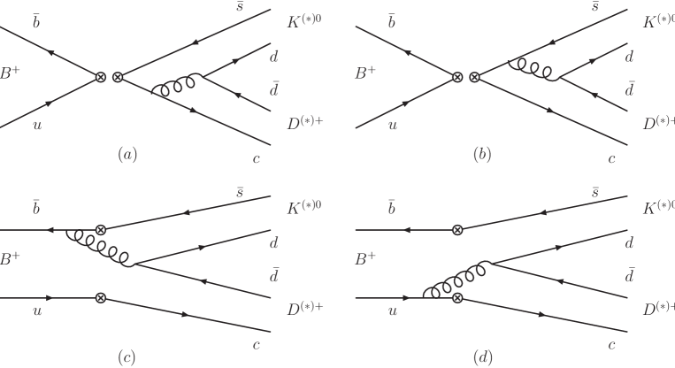
FIG. 1.: Diagrams for $B^{+}\to D^{(*)+}K^{(*)0}$ decays. The factorizable diagrams (a), (b) contribute to $F$, and nonfactorizable (c), (d) contribute to $M$.

REFERENCES

• [1] M. Wirbel, B. Stech, M. Bauer, Z. Phys. C29, 637 (1985); M. Bauer, B. Stech, M. Wirbel, Z. Phys. C34, 103 (1987); L.-L. Chau, H.-Y. Cheng, W.K. Sze, H. Yao, B. Tseng, Phys. Rev. D43, 2176 (1991), Erratum: D58, 019902 (1998).
• [2] A. Ali, G. Kramer and C.D. LΓΌ, Phys. Rev. D58, 094009 (1998); C.D. LΓΌ, Nucl. Phys. Proc. Suppl. 74, 227-230 (1999); Y.-H. Chen, H.-Y. Cheng, B. Tseng, K.-C. Yang, Phys. Rev. D60, 094014 (1999); H.-Y. Cheng and K.-C. Yang, Phys. Rev. D62, 054029 (2000).
• [3] H.Y. Cheng, H-n. Li, and K.C. Yang, Phys. Rev. D 60, 094005 (1999).
• [4] T.W. Yeh and H-n. Li, Phys. Rev. D 56, 1615 (1997).
• [5] M. Beneke, G. Buchalla, M. Neubert, C.T. Sachrajda, Phys. Rev. Lett. 83, 1914 (1999); Nucl. Phys. B591, 313 (2000).
• [6] Y.-Y. Keum, H.-n. Li and A. I. Sanda, Phys. Lett. B504, 6 (2001); Phys. Rev. D63, 054008 (2001).
• [7] C.-D. LΓΌ, K. Ukai and M.-Z. Yang, Phys. Rev. D63, 074009 (2001); C.-D. LΓΌ, pp. 173-184, Proceedings of International Conference on Flavor Physics (ICFP 2001), World Scientific, 2001, hep-ph/0110327.
• [8] G.P. Lepage and S.J. Brodsky, Phys. Lett. B 87, 359 (1979).
• [9] G.P. Lepage and S.J. Brodsky, Phys. Rev. D 22, 2157 (1980).
• [10] C.-H. V. Chang and H.-n. Li, Phys. Rev. D55, 5577 (1997); T.-W. Yeh and H.-n. Li, Phys. Rev. D56, 1615 (1997).
• [11] H.-n. Li, Phys. Rev. D64, 014019 (2001); S. Mishima, Phys. Lett. B521, 252 (2001); E. Kou and A.I. Sanda, Phys. Lett. B525, 240 (2002); C.-H. Chen, Y.-Y. Keum, and H.-n. Li, Phys. Rev. D64, 112002 (2001); C.-D. LΓΌ and M.Z. Yang, Eur. Phys. J. C23, 275 (2002); A.I. Sanda and K. Ukai, Prog. Theor. Phys. 107, 421 (2002); C.-H. Chen, Y.-Y. Keum, and H.-n. Li, Phys. Rev. D66, 054013 (2002); M. Nagashima and H.-n. Li, hep-ph/0202127; Y.-Y. Keum, hep-ph/0209002; hep-ph/0209208(to appear in PRL); hep-ph/0210127; Y.-Y. Keum and A. I. Sanda, Phys.Rev. D 67, 054009 (2003).
• [12] C.D. LΓΌ, Eur. Phys. J. C24, 121 (2002); Y. Li, C.D. LΓΌ, J.Phys. G29 2115 (2003); hep-ph/0305278; hep-ph/0308243; C.D. LΓΌ, K. Ukai, Eur.Phys.J. C28 305 (2003).
• [13] H.-n. Li and B. Tseng, Phys. Rev. D57, 443 (1998).
• [14] H.-n. Li, Phys. Rev. D 66, 094010 (2002); H.-n. Li, K. Ukai, Phys. Lett. B 555, 197 (2003).
• [15] G. Buchalla, A. J. Buras and M. E. Lautenbacher, Rev. Mod. Phys. 68, 1125(1996).
• [16] Review of Particle Physics, K. Hagiwara et al., Phys. Rev. D66, 010001 (2002).
• [17] T. Kurimoto, H.-n. Li, and A. I. Sanda, Phys. Rev. D 67, 054028 (2003).
• [18] Y.-Y. Keum, T. Kurimoto, H.-N. Li, C.-D. LΓΌ, A.I. Sanda, hep-ph/0305335.
• [19] P. Ball, JHEP, 09, 005, (1998); JHEP, 01, 010, (1999).
• [20] P. Ball, V.M. Braun, Y. Koike, and K. Tanaka, Nucl. Phys. B 529, 323 (1998); P. Ball, V. M. Braun, hep-ph/9808229.
• [21] Particle Data Group, Phys. Rev. D66, Part I (2002).
• [22] J.D. Bjorken, Nucl. Phys. B (Proc. Suppl.) 11, 325 (1989).
• [23] C.-H. Chen and H.-n. Li, Phys. Rev. D63, 014003 (2001).
• [24] H.-n. Li, B. Melic, Eur. Phys. J. C11, 695 (1999).
Refer to caption