Abstract

The leading corrections to electroweak precision observables in the MSSM with non-minimal flavor violation (NMFV) are calculated and the effects on $M_{W}$ and $\sin^{2}\theta_{\mathrm{eff}}$ are analyzed. The corrections are obtained by evaluating the full one-loop contributions from the third and second generation scalar quarks, including the mixing in the scalar top and charm, as well as in the scalar bottom and strange sector. Furthermore the leading corrections to the mass of the lightest MSSM Higgs boson, $m_{h}$, is obtained. The electroweak one-loop contribution to $M_{W}$ can amount up to $140\,\,\mathrm{MeV}$ and up to $70\times 10^{-5}$ for $\sin^{2}\theta_{\mathrm{eff}}$, allowing to set limits on the NMFV parameters. The corrections for $m_{h}$ are not significant for moderate generation mixing.

1 Introduction

Supersymmetric theories of the strong and electroweak interactions, like the Minimal Supersymmetric Standard Model (MSSM) [1] as the theoretically favored extension of the Standard Model (SM), predict the existence of scalar partners $\tilde{f}_{L},\tilde{f}_{R}$ to each SM chiral fermion, and of spin-1/2 partners to the gauge and Higgs bosons. So far, the direct search for SUSY particles could only set lower bounds of ${\cal O}(100)$ GeV on their masses [2]. In a similar way, the search for MSSM Higgs bosons resulted in lower limits of about $90\,\,\mathrm{GeV}$ for the neutral and $80\,\,\mathrm{GeV}$ for the charged Higgs particles [4].

An alternative way, as compared to the direct search for SUSY or Higgs particles, is to probe SUSY via virtual effects of the additional non-standard particles to precision observables. This requires very high precision of the experimental results as well as of the theoretical predictions. A predominant role in this respect has to be assigned to the $\rho$-parameter [5], with loop contributions $\Delta\rho$ through vector-boson self-energies constituting the leading process-independent quantum corrections to electroweak precision observables, such as the prediction for $\Delta r$ in the $M_{W}$–$M_{Z}$ interdependence and the effective leptonic weak mixing angle, $\sin^{2}\theta_{\mathrm{eff}}$.

Radiative corrections to the electroweak precision observables within the MSSM, originating from the virtual presence of scalar fermions, charginos, neutralinos, and Higgs bosons, have been discussed at the one-loop level in [6, 7], providing the full one-loop corrections. More recently, also the leading two-loop contributions in ${\cal O}(\alpha\alpha_{s})$ to $\Delta\rho$ from quarks, squarks, gluons, and gluinos have been obtained [8] as well as the gluonic two-loop corrections to the $M_{W}$–$M_{Z}$ interdependence [9]. Contrary to the SM case, these two-loop strong corrections turned out to increase the one-loop contributions, leading to an enhancement of up to 35% [8]. Most recently, the leading two-loop contributions to $\Delta\rho$ at ${\cal O}(\alpha_{t}^{2})$, ${\cal O}(\alpha_{t}\alpha_{b})$, ${\cal O}(\alpha_{b}^{2})$, i.e. the leading two-loop contributions involving the top and bottom Yukawa couplings, have been evaluated [10]. They affect $M_{W}$ and $\sin^{2}\theta_{\mathrm{eff}}$ by shifts reaching $12\,\,\mathrm{MeV}$ and $5\times 10^{-5}$, respectively.

At the quantum level, the Higgs sector of the MSSM is considerably affected by loop contributions and makes $m_{h}$ yet another sensitive observable. Precise predictions for the mass $m_{h}$ of the lightest Higgs boson $h$ and its couplings to other particles in terms of the relevant SUSY parameters are necessary in order to determine the discovery and exclusion potential of the upgraded Tevatron, and for physics at the LHC and a future linear collider, where high-precision measurements of the Higgs-boson(s) profile will become feasible [11, 12, 13].

Radiative corrections to the Higgs-boson masses in the ${\cal CP}$-conserving MSSM with minimal flavor violation (MFV) are meanwhile quite advanced. Besides the full one-loop corrections [14, 15], the two-loop corrections have been evaluated in the effective-potential method [16, 17, 18, 19], the renormalization-group approach [20], and the Feynman-diagrammatic approach [21, 22, 23] (see [24, 25] for a comparison), providing all leading two-loop contributions available by now [26]. However, the impact of non-minimal flavor violation (NMFV) on the MSSM Higgs-boson masses and mixing angles, entering already at the one-loop level, has not been explored so far, although effects from possible NMFV on Higgs-boson decays were investigated in [27, 28]. Simultaneously, effects of NMFV enter also the electroweak precision observables at the one-loop level, but have never been analyzed as yet. Hence, we study in this paper the consequences from NMFV for both the electroweak precision observables and the MSSM lightest Higgs-boson mass $m_{h}$.

The most general flavor structure of the soft SUSY-breaking sector with flavor non-diagonal terms would induce large flavor-changing neutral-currents, contradicting the experimental results [2]. Attempts to avoid this kind of problem include flavor-blind SUSY-breaking scenarios, like minimal Supergravity or gauge-mediated SUSY-breaking. In these scenarios, the sfermion-mass matrices are flavor diagonal in the same basis as the quark matrices at the SUSY-breaking scale. However, a certain amount of flavor mixing is generated due to the renormalization-group evolution from the SUSY-breaking scale down to the electroweak scale. Estimates of this radiatively induced off-diagonal squark-mass terms indicate that the largest entries are those connected to the SUSY partners of the left-handed quarks [30, 29], generically denoted as $\Delta_{LL}$. Those off-diagonal soft SUSY-breaking terms scale with the square of diagonal soft SUSY-breaking masses $M_{\mathrm{SUSY}}$, whereas the $\Delta_{LR}$ and $\Delta_{RL}$ terms scale linearly, and $\Delta_{RR}$ with zero power of $M_{\mathrm{SUSY}}$. Therefore, usually the hierarchy $\Delta_{LL}\gg\Delta_{LR,RL}\gg\Delta_{RR}$ is realized. It was also shown in [30, 29] that mixing between the third and second generation squarks can be numerically significant due to the involved third-generation Yukawa couplings. On the other hand, there are strong experimental bounds on squark mixing involving the first generation, coming from data on $K^{0}$–$\bar{K}^{0}$ and $D^{0}$–$\bar{D}^{0}$ mixing [31, 32].

The analytical results obtained in this paper have been derived for the general case of mixing between the third and second generation of squarks, i.e. all NMFV contributions, $\Delta_{LL,LR,RL,RR}$, can be chosen independently in the $\tilde{t}/\tilde{c}$ and in the $\tilde{b}/\tilde{s}$ sector (corrections from the first-generation squarks are not considered, for reasons mentioned above). The numerical analysis of NMFV effects, however, and the illustration of the behavior of $m_{h}$ and electroweak observables are performed for the simpler, but well motivated, scenario (also chosen in [28]) where only mixing between $\tilde{t}_{L}$ and $\tilde{c}_{L}$ as well as between $\tilde{b}_{L}$ and $\tilde{s}_{L}$ is considered, with $\Delta_{LL}^{t}$ and $\Delta_{LL}^{b}$ as the only flavor off-diagonal entries in the squark-mass matrices.

The paper is organized as follows. In Sect. 2 we review the MSSM with NMFV and set up the notation. Corrections to the lightest MSSM Higgs-boson mass at the one-loop level arising from NMFV are presented in Sect. 3. Analytical and numerical results for $\Delta\rho$ are given in Sect. 4, together with a numerical analysis of the full one-loop effects from scalar quarks on $M_{W}$ and $\sin^{2}\theta_{\mathrm{eff}}$. Sect. 5 is devoted to the conclusions. Finally, in the appendix, we list the set of Feynman rules for the general case of NMFV.

2 Non-minimal flavor violation in the MSSM

As explained in the introduction, our analytical results are obtained for a general mixing of the third and second generation of scalar quarks. The squark mass matrices in the basis of $(\tilde{c}_{L},\tilde{t}_{L},\tilde{c}_{R},\tilde{t}_{R})$ and $(\tilde{s}_{L},\tilde{b}_{L},\tilde{s}_{R},\tilde{b}_{R})$  are given by

$$M_{\tilde{u}}^{2} = \left(\begin{array}[]{cccc}M_{\tilde{L}_{c}}^{2}&\Delta_{LL}^{t}&m_{c}X_{c}&\Delta_{LR}^{t}\\[3.00003pt] \Delta_{LL}^{t}&M_{\tilde{L}_{t}}^{2}&\Delta_{RL}^{t}&m_{t}X_{t}\\[5.0pt] m_{c}X_{c}&\Delta_{RL}^{t}&M_{\tilde{R}_{c}}^{2}&\Delta_{RR}^{t}\\[3.00003pt] \Delta_{LR}^{t}&m_{t}X_{t}&\Delta_{RR}^{t}&M_{\tilde{R}_{t}}^{2}\end{array}\right)$$ (5)

$$M_{\tilde{d}}^{2} = \left(\begin{array}[]{cccc}M_{\tilde{L}_{s}}^{2}&\Delta_{LL}^{b}&m_{s}X_{s}&\Delta_{LR}^{b}\\[3.00003pt] \Delta_{LL}^{b}&M_{\tilde{L}_{b}}^{2}&\Delta_{RL}^{b}&m_{b}X_{b}\\[5.0pt] m_{s}X_{s}&\Delta_{RL}^{b}&M_{\tilde{R}_{s}}^{2}&\Delta_{RR}^{b}\\[3.00003pt] \Delta_{LR}^{b}&m_{b}X_{b}&\Delta_{RR}^{b}&M_{\tilde{R}_{b}}^{2}\end{array}\right)$$ (10)

with

$$M_{\tilde{L}_{q}}^{2} = M_{\tilde{Q}_{q}}^{2}+m_{q}^{2}+\cos 2\beta\hskip 2.84526ptM_{Z}^{2}(T_{3}^{q}-Q_{q}s_{W}^{2})$$

$$M_{\tilde{R}_{q}}^{2} = M_{\tilde{U}_{q}}^{2}+m_{q}^{2}+\cos 2\beta\hskip 2.84526ptM_{Z}^{2}Q_{q}s_{W}^{2}~{}(q=t,c)$$

$$M_{\tilde{R}_{q}}^{2} = M_{\tilde{D}_{q}}^{2}+m_{q}^{2}+\cos 2\beta\hskip 2.84526ptM_{Z}^{2}Q_{q}s_{W}^{2}~{}(q=b,s)$$

$$X_{q} = A_{q}-\mu(\tan\beta)^{-2T_{3}^{q}}$$ (11)

where $m_{q}$, $Q_{q}$ and $T_{3}^{q}$ are the mass, electric charge and weak isospin of the quark $q$. $M_{\tilde{Q}_{q}}$, $M_{\tilde{U}_{q}}$, $M_{\tilde{D}_{q}}$ are the soft SUSY-breaking parameters. The $SU(2)$ structure of the model requires $M_{\tilde{Q}_{q}}$ to be equal for $\tilde{t}$ and $\tilde{b}$ as well as for $\tilde{c}$ and $\tilde{s}$. The expressions furthermore contain the $Z$ and $W$ boson masses $M_{Z,W}$; the electroweak mixing angle in $s_{W}=\sin\theta_{W}$, $c_{W}=\cos\theta_{W}$; the trilinear Higgs couplings $A_{q}\,(q=t,b,c,s)$ to $\tilde{t}$, $\tilde{b}$, $\tilde{c}$, $\tilde{s}$; the Higgsino mass parameter $\mu$, and $\tan\beta=v_{2}/v_{1}$.

In order to diagonalize the two $4\times 4$ squark mass matrices, two $4\times 4$ rotation matrices, $R_{\tilde{u}}$ and $R_{\tilde{d}}$, are needed,

$$\tilde{u}_{\alpha}\;=\;R_{\tilde{u}}^{\alpha,j}\left(\begin{array}[]{c}\tilde{c}_{L}\\ \tilde{t}_{L}\\ \tilde{c}_{R}\\ \tilde{t}_{R}\end{array}\right)_{j}~{},~{}~{}~{}~{}\tilde{d}_{\alpha}\;=\;R_{\tilde{d}}^{\alpha,j}\left(\begin{array}[]{c}\tilde{s}_{L}\\ \tilde{b}_{L}\\ \tilde{s}_{R}\\ \tilde{b}_{R}\end{array}\right)_{j}~{},$$ (12)

yielding the diagonal mass-squared matrices as follows,

$${\rm diag}\{m_{\tilde{u}_{1}}^{2},m_{\tilde{u}_{2}}^{2},m_{\tilde{u}_{3}}^{2},m_{\tilde{u}_{4}}^{2}\}^{\alpha,\beta} = R_{\tilde{u}}^{\alpha,i}\;\left(M_{\tilde{u}}^{2}\right)_{i,j}\;(R_{\tilde{u}}^{\beta,j})^{\dagger}~{},$$ (13)

$${\rm diag}\{m_{\tilde{d}_{1}}^{2},m_{\tilde{d}_{2}}^{2},m_{\tilde{d}_{3}}^{2},m_{\tilde{d}_{4}}^{2}\}^{\alpha,\beta} = R_{\tilde{d}}^{\alpha,i}\;\left(M_{\tilde{d}}^{2}\right)_{i,j}\;(R_{\tilde{d}}^{\beta,j})^{\dagger}~{}.$$ (14)

Feynman rules that involve two scalar quarks can be obtained from the rules given in the $\tilde{f}_{L},\tilde{f}_{R}$ basis by applying the corresponding rotation matrix ($\tilde{q}=\tilde{u},\tilde{d}$),

$$V(X\tilde{q}_{\alpha}\tilde{q}_{\beta}^{\prime})\;=\;R_{\tilde{q}}^{\alpha,i}\;R_{\tilde{q}^{\prime}}^{\beta,j}\;V(X\tilde{q}_{i}\tilde{q}^{\prime}_{j})~{}.$$ (15)

Thereby $V(X\tilde{q}_{i}\tilde{q}^{\prime}_{j})$ denotes a generic vertex in the $\tilde{f}_{L},\tilde{f}_{R}$ basis, and $V(X\tilde{q}_{\alpha}\tilde{q}_{\beta}^{\prime})$ is the vertex in the NMFV mass-eigenstate basis. The Feynman rules for the vertices needed for our applications, i.e. the interaction of one and two Higgs or gauge bosons with two squarks, can be found in the appendix. This new set of generalized vertices has been implemented into the program packages FeynArts/FormCalc[35] extending the previous MSSM model file [36] . The extended FeynArts version was used for the evaluation of the Feynman diagrams along this paper to obtain the general analytical results.

For the numerical analysis we are more specific and consider the simpler scenario with mixing only between the left-handed components of $\tilde{t},\tilde{c}$ and $\tilde{b},\tilde{s}$, as explained in the introduction. The only flavor off-diagonal entries in the squark-mass matrices are normalized according to $\Delta_{LL}^{t,b}=\lambda^{t,b}M_{\tilde{Q}_{3}}M_{\tilde{Q}_{2}}$, following [30, 31, 32] , where $M_{\tilde{Q}_{3},\tilde{Q}_{2}}$ are the soft SUSY-breaking masses for the $SU(2)$ squark doublet in the third and second generation. NMFV is thus parametrized in terms of the dimensionless quantities $\lambda^{t}$ and $\lambda^{b}$ (see [31, 32, 33, 34] for experimentally allowed ranges). The case of $\lambda^{t}=\lambda^{b}=0$ corresponds to the MSSM with minimal flavor violation (MFV). In detail, we have

$$\Delta_{LL}^{t} =\lambda^{t}M_{\tilde{L}_{t}}M_{\tilde{L}_{c}}\,, \Delta_{LR}^{t}=\Delta_{RL}^{t}=\Delta_{RR}^{t} =0\,,$$

$$\Delta_{LL}^{b} =\lambda^{b}M_{\tilde{L}_{b}}M_{\tilde{L}_{s}}\,, \Delta_{LR}^{b}=\Delta_{RL}^{b}=\Delta_{RR}^{b} =0\,,$$ (16)

for the entries in the matrices (5) and (10).

For the sake of simplicity, we have assumed in our numerical analysis the same flavor mixing parameter in the $\tilde{t}-\tilde{c}$ and $\tilde{b}-\tilde{s}$ sectors, $\lambda=\lambda^{t}=\lambda^{b}$. It should be noted in this respect that LL blocks of the up-squark and down-squark mass matrices are not independent because of the $SU(2)$ gauge invariance; they are related trough the CKM mass matrix [32], which also implies that a large difference between these two parameters is not allowed.

3 The mass of the lightest Higgs boson

The higher-order corrected masses $m_{h},\,m_{H}$ of the ${\cal CP}$-even neutral Higgs bosons $h,H$ correspond to the poles of the $h,H$-propagator matrix. In terms of its inverse, it is given by

$$\left(\Delta_{\rm Higgs}\right)^{-1}=-i\left(\begin{array}[]{cc}p^{2}-m_{H,{\rm tree}}^{2}+\hat{\Sigma}_{HH}(p^{2})&\hat{\Sigma}_{hH}(p^{2})\\[5.0pt] \hat{\Sigma}_{hH}(p^{2})&p^{2}-m_{h,{\rm tree}}^{2}+\hat{\Sigma}_{hh}(p^{2})\end{array}\right),$$ (17)

where $m_{h,{\rm tree}},m_{H,{\rm tree}}$ are the tree-level $h,H$ masses, and $\hat{\Sigma}(p^{2})$ denote the renormalized Higgs-boson self-energies for a general momentum $p$. Determining the poles of the matrix $\Delta_{\rm Higgs}$ in (17) is equivalent to solving the equation

$$\left[p^{2}-m_{h,{\rm tree}}^{2}+\hat{\Sigma}_{hh}(p^{2})\right]\left[p^{2}-m_{H,{\rm tree}}^{2}+\hat{\Sigma}_{HH}(p^{2})\right]-\left[\hat{\Sigma}_{hH}(p^{2})\right]^{2}=0\,.$$ (18)

The status of the available results for the self-energy contributions to (17) has been summarized in the introduction (see also [26] for a review).

Figure 1: Feynman diagrams for the squark contributions to the Higgs boson self-energies and for the tadpole contributions.

Within the MSSM with MFV, the dominant one-loop contributions to the self-energies in (17) result from the Yukawa part of the theory (i.e. neglecting the gauge couplings); they are described by loop diagrams involving third-generation quarks and squarks. Within the MSSM with NMFV, the squark loops have to be modified by introducing the generation-mixed squarks, as given in (12). The contributing Feynman diagrams are illustrated in Fig. 1. The leading terms are obtained by evaluating the contributions to the renormalized Higgs-boson self-energies at zero external momentum, $\hat{\Sigma}_{s}(0),s=hh,hH,HH$. Thereby, the renormalized self-energies are given by

$$\hat{\Sigma}_{s}=\Sigma_{s}-\delta V_{s}~{},~{}~{}s=hh\,,hH\,,HH\,.$$ (19)

$\Sigma_{s}$ are the unrenormalized Higgs boson self-energies, and $\delta V_{s}$ are the counter terms for the various coefficients in the quadratic part of the Higgs potential,

$$\delta V_{hh} = \delta M_{A}^{2}(c_{\alpha}c_{\beta}+s_{\alpha}s_{\beta})^{2}$$

$$-T_{1}\frac{e}{2s_{W}M_{W}}(-2c_{\alpha}s_{\alpha}s_{\beta}^{3}+c_{\beta}(-c_{\alpha}^{2}s_{\beta}^{2}+s_{\alpha}^{2}(1+s_{\beta}^{2})))$$

$$-T_{2}\frac{e}{2s_{W}M_{W}}(-2c_{\alpha}s_{\alpha}c_{\beta}^{3}+s_{\beta}(c_{\alpha}^{2}(1+c_{\beta}^{2})-s_{\alpha}^{2}c_{\beta}^{2}))\,,$$

$$\delta V_{HH} = \delta M_{A}^{2}(s_{\alpha}c_{\beta}-c_{\alpha}s_{\beta})^{2}$$

$$-T_{1}\frac{e}{2s_{W}M_{W}}(-c_{\beta}s_{\alpha}^{2}s_{\beta}^{2}+2s_{\alpha}c_{\alpha}s_{\beta}^{3}+c_{\alpha}^{2}c_{\beta}(1+s_{\beta}^{2}))$$

$$-T_{2}\frac{e}{2s_{W}M_{W}}(2s_{\alpha}c_{\alpha}c_{\beta}^{3}-c_{\alpha}^{2}c_{\beta}^{2}s_{\beta}+(1+c_{\beta}^{2})s_{\alpha}^{2}s_{\beta})\,,$$

$$\delta V_{hH} = \delta M_{A}^{2}(s_{\beta}c_{\beta}(s_{\alpha}^{2}-c_{\alpha}^{2})+s_{\alpha}c_{\alpha}(c_{\beta}^{2}-s_{\beta}^{2}))$$ (20)

$$-T_{1}\frac{e}{2s_{W}M_{W}}(s_{\beta}^{3}(c_{\alpha}^{2}-s_{\alpha}^{2})-s_{\alpha}c_{\alpha}c_{\beta}(1+2s_{\beta}^{2}))$$

$$-T_{2}\frac{e}{2s_{W}M_{W}}(c_{\beta}^{3}(c_{\alpha}^{2}-s_{\alpha}^{2})+s_{\alpha}c_{\alpha}s_{\beta}(1+2c_{\beta}^{2}))\,.$$

These expressions involve $s_{\alpha}\equiv\sin\alpha\hskip 2.84526pt$, $c_{\alpha}\equiv\cos\alpha\hskip 2.84526pt$ of the angle $\alpha$ diagonalizing the lowest-order Higgs-boson mass matrix, the $A$-boson mass counter term, and the tadpoles $T_{1}$ and $T_{2}$. In the on-shell renormalization scheme (in the leading Yukawa approximation) they are determined by

$$\delta M_{A}^{2}=\Sigma_{A}(0)$$ (21)

$${\mbox{and}}\hskip 142.26378ptT_{1}=T_{H\big{|}\alpha\to 0}~{},\qquad T_{2}=T_{h\big{|}\alpha\to 0}\,,$$ (22)

where $T_{h,H}$ correspond to the tadpole diagrams displayed in Fig. 1.

Here we restrict ourselves to the dominant Yukawa contributions resulting from the top and $t/\tilde{t}$ (and $c/\tilde{c}$) sector. Corrections from $b$ and $b/\tilde{b}$ (and $s/\tilde{s}$) could only be important for very large values of $\tan\beta$, $\tan\beta\;\raisebox{-3.00003pt}{$\stackrel{{\scriptstyle\displaystyle>}}{{\sim}}$}\;m_{t}/m_{b}$, which we do not consider here. The analytical result of the renormalized Higgs boson self-energies, based on the general $4\times 4$ structure of the $\tilde{t}/\tilde{c}$ mass matrix, has then been implemented into the Fortran code FeynHiggs2.1 [37] that includes all existing higher-order corrections (of the MFV MSSM). All data shown in this letter has then been obtained with the help of FeynHiggs2.1.

The results for the lightest MSSM Higgs-boson mass, including all available corrections also at the two-loop level, are presented for five benchmark scenarios defined in [38], named “$m_{h}^{\rm max}$” (to maximize the lightest Higgs boson mass), “constrained $m_{h}^{\rm max}$” (labeled as “$X_{t}/M_{\mathrm{SUSY}}=-2$”), “no-mixing” (with no mixing in the MFV $\tilde{t}$ sector), “gluophobic Higgs” (with reduced $ggh$ coupling), and “small $\alpha_{\rm eff}$” scenario (with reduced $hb\bar{b}$ and $h\tau^{+}\tau^{-}$ couplings). For all these benchmark scenarios the soft SUSY-breaking parameters in the three generations of scalar quarks are equal,

$$M_{\mathrm{SUSY}}=M_{\tilde{Q}_{q}}=M_{\tilde{U}_{q}}=M_{\tilde{D}_{q}}~{},$$ (23)

as well as all the trilinear couplings, $A_{s}=A_{b}=A_{c}=A_{t}$. Despite these simplifications, the five scenarios can show quite different behavior concerning observables in the Higgs sector [38].

In Fig. 2 we illustrate the dependence of $m_{h}$ on $\lambda(=\lambda^{t})$ in all five benchmark scenarios. $M_{A}$ has been fixed to $M_{A}=500\,\,\mathrm{GeV}$, and $\tan\beta$ is set to $\tan\beta=5$ (left) or $\tan\beta=20$ (right). All scenarios show a similar behavior. For small to moderate allowed values of $\lambda$ the variation of $m_{h}$ is small. Only for large values (around 0.5 in the gluophobic Higgs scenario, and around 0.9 in the other four scenarios) the variation of $m_{h}$ can be quite strong, up to the ${\cal O}(5\,\,\mathrm{GeV})$. In the gluophobic Higgs scenario unphysical values for the scalar quark masses are reached already for smaller values of $\lambda$, since $M_{\mathrm{SUSY}}$ is quite low in this scenario (see [38] for details). Values of $\lambda$ above $0.5$ imply forbidden values for the squark masses in this scenario. In all cases except for the small $\alpha_{\rm eff}$ scenario the lightest Higgs boson mass turns out to be reduced. In the small $\alpha_{\rm eff}$ scenario it can be enhanced by up to $2\,\,\mathrm{GeV}$. Considering that large values of $\lambda$ are in conflict with FCNC data, the impact of NMFV on $m_{h}$ is in general rather small. Conversely, independent of low-energy FCNC data on flavor mixing, high values of $\lambda$ can be constrained by the experimental lower bound on $m_{h}$ [4].

Figure 2: The variation of $m_{h}$ with $\lambda=\lambda^{t}$ is shown in five benchmark scenarios [38]. $M_{A}$ has been fixed to $M_{A}=500\,\,\mathrm{GeV}$, and $\tan\beta$ is set to $\tan\beta=5$ (left panel) or $\tan\beta=20$ (right panel).

4 $\Delta\rho$ and electroweak precision observables

One important consequence of flavor mixing through the flavor non-diagonal entries in the squark mass matrices (5,10) is to generate large splittings between the squark-mass eigenvalues. The loop contribution to the electroweak $\rho$ parameter,

$$\Delta\rho=\frac{\Sigma_{Z}(0)}{M_{Z}^{2}}-\frac{\Sigma_{W}(0)}{M_{W}^{2}},$$ (24)

with the unrenormalized $Z$ and $W$ boson self-energies at zero momentum, $\Sigma_{Z,W}(0)$, represents the leading universal corrections to the electroweak precision observables induced by mass splitting between partners in isospin doublets [5] and is thus sensitive to the mass-splitting effects induced by non-minimal flavor mixing. Precisely measured observables [39] like the $W$ boson mass, $M_{W}$, and the effective leptonic mixing angle, $\sin^{2}\theta_{\mathrm{eff}}$, are affected by shifts according to

$$\delta M_{W}\approx\frac{M_{W}}{2}\frac{c_{W}^{2}}{c_{W}^{2}-s_{W}^{2}}\Delta\rho,\quad\delta\sin^{2}\theta_{\mathrm{eff}}\approx-\frac{c_{W}^{2}s_{W}^{2}}{c_{W}^{2}-s_{W}^{2}}\Delta\rho.$$ (25)

Within the MSSM with MFV, the dominant correction from SUSY particles at the one-loop level arises from the $\tilde{t}$ and $\tilde{b}$ contributions. Explicit expressions can be found in [10], together with the SUSY-QCD and SUSY-EW corrections at two-loop order.

Beyond the $\Delta\rho$ approximation, the shift in $M_{W}$ caused by a variation of $\Delta r$ can be written as follows,

$$\delta M_{W}=-\frac{M_{W}}{2}\frac{s_{W}^{2}}{c_{W}^{2}-s_{W}^{2}}\delta(\Delta r)\,.$$ (26)

As far as $\delta\Delta r$ originates from loop contributions to the self energies only, it is given by

$$\delta(\Delta r)=\Sigma_{\gamma}^{\prime}(0)-\frac{c_{W}^{2}}{s_{W}^{2}}\left(\frac{\Sigma_{Z}(M_{Z}^{2})}{M_{Z}^{2}}-\frac{\Sigma_{W}(M_{W}^{2})}{M_{W}^{2}}\right)+\frac{\Sigma_{W}(0)-\Sigma_{W}(M_{W}^{2})}{M_{W}^{2}}~{},$$ (27)

with $\Sigma^{\prime}=\frac{\partial}{\partial q^{2}}\Sigma(q^{2})$. In the case considered here, the self-energies in (27) stand for the set of squark-loop contributions. Likewise the induced shift in the effective mixing angle reads as follows,

$$\delta\sin^{2}\theta_{\mathrm{eff}}=\frac{c_{W}^{2}\,s_{W}^{2}}{c_{W}^{2}-s_{W}^{2}}\delta(\Delta r)-s_{W}c_{W}\left[\frac{\Sigma_{\gamma Z}(M_{Z}^{2})}{M_{Z}^{2}}-\frac{c_{W}}{s_{W}}\left(\frac{\Sigma_{Z}(M_{Z}^{2})}{M_{Z}^{2}}-\frac{\Sigma_{W}(M_{W}^{2})}{M_{W}^{2}}\right)\right]~{},$$ (28)

again evaluated for the squark-loop contributions in our case.

4.1 Analytical results for $\Delta\rho$

Here we consider the supersymmetric NMFV contributions to $\Delta\rho$ resulting from squarks based on the general $4\times 4$ mass matrix for both the $\tilde{t}/\tilde{c}$ and the $\tilde{b}/\tilde{s}$ sector, visualized by the Feynman diagrams in Fig. 3. These contributions will be denoted as $\Delta\rho^{\tilde{q}}$. The analytical one-loop result for $\Delta\rho^{\tilde{q}}$ has been implemented into the Fortran code FeynHiggs2.1 [37].

\psfrag{lam}{{\scriptsize$\lambda$}}\psfrag{lamu}{{\scriptsize$\lambda_{\tilde{u}}$}}\psfrag{lamd}{{\scriptsize$\lambda_{\tilde{d}}$}}\psfrag{lamt}{{\scriptsize$\lambda_{t}$}}\psfrag{lamb}{{\scriptsize$\lambda_{b}$}}\psfrag{dr}{{\scriptsize$\Delta\rho$}}\psfrag{MSusy}{{\scriptsize$M_{\rm{\tiny{SUSY}}}$ [GeV]}}\psfrag{mhmax}{{\scriptsize$m_{h}^{\mbox{\tiny{max}}}$ scenario}}\psfrag{nomix}{{\scriptsize no-mixing scenario }}\psfrag{mhmax1000}{{\scriptsize$m_{h}^{\mbox{\tiny{max}}},M_{\mbox{SUSY }}=1\,\,\mathrm{TeV}$}}\psfrag{nomix1000}{{\scriptsize no-mixing, $M_{\mbox{SUSY }}=1\,\,\mathrm{TeV}$}}\psfrag{mhmax2000}{{\scriptsize$m_{h}^{\mbox{\tiny{max}}},M_{\mbox{SUSY }}=2\,\,\mathrm{TeV}$}}\psfrag{nomix2000}{{\scriptsize no-mixing, $M_{\mbox{SUSY }}=2\,\,\mathrm{TeV}$}}\psfrag{mhmaxep}{{\scriptsize$m_{h}^{\mbox{\tiny{max}}},\,$ $\epsilon$ positive}}\psfrag{mhmaxem}{{\scriptsize$m_{h}^{\mbox{\tiny{max}}},\,$ $\epsilon$ negative}}\psfrag{nomixep}{{\scriptsize no-mixing,\,$\epsilon$ positive}}\psfrag{nomixem}{{\scriptsize no-mixing, \,$\epsilon$ negative}}\psfrag{nomix}{{\scriptsize no-mixing scenario }}\psfrag{dmw}{\rotatebox{90.0}{\footnotesize$\delta M_{W}\,[GeV]$}}\psfrag{dst}{\rotatebox{90.0}{\hskip 14.22636pt\footnotesize$\delta\sin^{2}\theta_{\mathrm{eff}}$ }}\psfrag{f1}{$f_{1}$}\psfrag{f2}{$f_{2}$}\includegraphics[width=384.1122pt,clip={}]{rhodia.ps}

Figure 3: Feynman diagrams for the squark contributions to the gauge boson self-energies.

The squark contribution $\Delta\rho^{\tilde{q}}$ can be decomposed according to

$$\Delta\rho^{\tilde{q}}=\Xi_{Z}+\Theta_{Z}+\Xi_{W}+\Theta_{W}\,,$$ (29)

where $\Xi$ and $\Theta$ correspond to different diagram topologies, i.e. to diagrams with trilinear and quartic couplings, respectively (see Fig. 3). The explicit expressions read as follows,

$$\Xi_{W} = \frac{3g^{2}}{8\pi^{2}M_{W}^{2}}\sum\limits_{a,b,c,d}\sum\limits_{\alpha,\beta}V_{\rm CKM}^{ab}V_{\rm CKM}^{cd}R_{\tilde{u}}^{\alpha a}R_{\tilde{u}}^{\alpha c}R_{\tilde{d}}^{\beta b}R_{\tilde{d}}^{\beta d}B_{00}(0,m_{\tilde{u}_{\alpha}}^{2},m_{\tilde{d}_{\beta}}^{2})\,,$$

$$\Theta_{W} = -\frac{3g^{2}}{32\pi^{2}M_{W}^{2}}\sum\limits_{a}\sum\limits_{\alpha}\left\{(R_{\tilde{u}}^{\alpha a})^{2}A_{0}(m_{\tilde{u}_{\alpha}}^{2})+(R_{\tilde{d}}^{\alpha a})^{2}A_{0}(m_{\tilde{d}_{\alpha}}^{2})\right\}\,,$$

$$\Xi_{Z} = -\frac{3g^{2}}{144c_{W}^{2}\pi^{2}M_{Z}^{2}}\sum\limits_{\alpha,\beta,\gamma,\delta}\Big{\{}\kappa_{\tilde{d}}(\gamma)R_{\tilde{d}}^{\alpha\gamma}R_{\tilde{d}}^{\beta\gamma}\kappa_{\tilde{d}}(\delta)R_{\tilde{d}}^{\alpha\delta}R_{\tilde{d}}^{\beta\delta}B_{00}(0,m_{\tilde{d}_{\alpha}}^{2},m_{\tilde{d}_{\beta}}^{2})$$

$$+\kappa_{\tilde{u}}(\gamma)R_{\tilde{u}}^{\alpha\gamma}R_{\tilde{u}}^{\beta\gamma}\kappa_{\tilde{u}}(\delta)R_{\tilde{u}}^{\alpha\delta}R_{\tilde{u}}^{\beta\delta}B_{00}(0,m_{\tilde{u}_{\alpha}}^{2},m_{\tilde{u}_{\beta}}^{2})\Big{\}}\,,$$

$$\Theta_{Z} = \frac{3g^{2}}{288c_{W}^{2}\pi^{2}M_{Z}^{2}}\sum\limits_{\alpha,\beta,\gamma,\delta}\left\{(\kappa_{\tilde{d}}(\gamma)^{2}(R_{\tilde{d}}^{\alpha\gamma})^{2}A_{0}(m_{\tilde{d}_{\alpha}}^{2})+\kappa_{\tilde{u}}(\gamma)^{2}(R_{\tilde{u}}^{\alpha\gamma})^{2}A_{0}(m_{\tilde{u}_{\alpha}}^{2})\right\}~{}.$$ (30)

Here the indices run from 1 to 2 for Latin letters, and from 1 to 4 for Greek letters. The expressions contain the one-point integral $A_{0}$ and the two-point integral $B_{00}$ in $B_{\mu\nu}(k)=g_{\mu\nu}\,B_{00}+k_{\mu}k_{\nu}B_{11}$ in the convention of [35]. The remaining constants $\kappa_{\tilde{u}}$ and $\kappa_{\tilde{d}}$ are defined as follows,

$$\kappa_{\tilde{d}}=\left(\begin{array}[]{c}3-2\,s_{W}^{2}\\ 3-2\,s_{W}^{2}\\ -2\,s_{W}^{2}\\ -2\,s_{W}^{2}\end{array}\right)~{},\qquad\qquad\kappa_{\tilde{u}}=\left(\begin{array}[]{c}-3+4\,s_{W}^{2}\\ -3+4\,s_{W}^{2}\\ 4\,s_{W}^{2}\\ 4\,s_{W}^{2}\end{array}\right)~{}.$$ (39)

The CKM matrix only affects $\Xi_{W}$. Corrections from the first-generation squarks are negligible due to their very small mass splitting. Non-minimal flavor mixing of the first generation with the other ones has been set to zero (see Sect. 2), but conventional CKM mixing is basically present. Although it is required for a UV finite result, it yields only negligibly small effects. Therefore, for simplification, we drop the first generation and restore the cancellation of UV divergences by a unitary $2\times 2$ matrix replacing the {23}-submatrix of the CKM matrix,

$$V_{\rm CKM}=\left(\begin{array}[]{cc}V_{cs}&V_{cb}\\ V_{ts}&V_{tb}\end{array}\right)=\left(\begin{array}[]{cc}\cos\epsilon&\sin\epsilon\\ -\sin\epsilon&\cos\epsilon\end{array}\right)~{},$$ (44)

with $|\epsilon|\approx 0.04$ close to the experimental entries [2] of the conventional CKM matrix.

In the SM (and also in the MSSM with $\lambda=\lambda^{t}=\lambda^{b}=0$) the choice of the sign of $\epsilon$ does not play a role. However, the situation changes when $\lambda\neq 0$ . In the expression for $\Delta\rho^{\tilde{q}}$ some terms linear in $\epsilon$ arise from the expansion of $\Xi_{W}$, and the sign of $\epsilon$ can affect the result significantly. The expansion of $\Xi_{W}$ can be expressed as,

$$\Xi_{W}=f_{0}+f_{1}\epsilon+f_{2}\epsilon^{2}+\ldots+f_{n}\epsilon^{n}+\ldots$$ (45)

where the coefficients $f_{i}(i=0,1,2,\ldots)$ are functions of the rotation matrices $R_{\tilde{q}}$ and the squarks masses $m_{\tilde{q}}$ and therefore, they depend implicitly of the flavor parameter $\lambda$. The explicit analytical expressions for the first terms are:

$$f_{0} = -\frac{3g^{2}}{8M_{W}^{2}\pi^{2}}\sum\limits_{\alpha,\beta}\left(R_{\tilde{d}}^{1\beta}R_{\tilde{u}}^{1\alpha}+R_{\tilde{d}}^{2\beta}R_{\tilde{u}}^{2\alpha}\right)^{2}B_{00}(0,m_{\tilde{u}_{\alpha}}^{2},m_{\tilde{d}_{\beta}}^{2})\,,$$

$$f_{1} = -\frac{3g^{2}}{4M_{W}^{2}\pi^{2}}\sum\limits_{\alpha,\beta}\left((R_{\tilde{u}}^{1\alpha})^{2}R_{\tilde{d}}^{1\beta}R_{\tilde{d}}^{2\beta}+R_{\tilde{u}}^{1\alpha}R_{\tilde{u}}^{2\alpha}(R_{\tilde{d}}^{2\beta})^{2}\right.$$

$$\left.-R_{\tilde{u}}^{1\alpha}R_{\tilde{u}}^{2\alpha}(R_{\tilde{d}}^{1\beta})^{2}-(R_{\tilde{u}}^{2\alpha})^{2}R_{\tilde{d}}^{1\beta}R_{\tilde{d}}^{2\beta}\right)B_{00}(0,m_{\tilde{u}_{\alpha}}^{2},m_{\tilde{d}_{\beta}}^{2})\,,$$

$$f_{2} = \frac{3g^{2}}{8M_{W}^{2}\pi^{2}}\sum\limits_{\alpha,\beta}\left((R_{\tilde{u}}^{1\alpha})^{2}(R_{\tilde{d}}^{1\beta})^{2}+(R_{\tilde{u}}^{1\alpha})^{2}(R_{\tilde{d}}^{2\beta})^{2}-(R_{\tilde{u}}^{2\alpha})^{2}(R_{\tilde{d}}^{1\beta})^{2}\right.$$ (46)

$$\left.-(R_{\tilde{u}}^{2\alpha})^{2}(R_{\tilde{d}}^{2\beta})^{2}+R_{\tilde{u}}^{1\alpha}R_{\tilde{u}}^{2\alpha}R_{\tilde{d}}^{1\beta}R_{\tilde{d}}^{2\beta}\right)B_{00}(0,m_{\tilde{u}_{\alpha}}^{2},m_{\tilde{d}_{\beta}}^{2})\,.$$

Since $\Delta\rho^{\tilde{q}}$ is a finite quantity, and the CKM matrix effects (and therefore, the $\epsilon$ dependence) only appear in $\Xi_{W}$, $f_{0}$ is the unique coefficient in the expansion that contributes to the cancellation of divergences in $\Delta\rho^{\tilde{q}}$. The coefficients $f_{1}$ and $f_{2}$ are finite and their $\lambda$ dependence is shown in Fig. 4. While $f_{1}=0$ for $\lambda=0$, $f_{2}$ is not exactly zero but its value is very small, around $5.5\times 10^{-5}$. This small value at $\lambda=0$ implies that the CKM effects in the MSSM with MFV are indeed negligible, which is in agreement with the universal assumptions in MFV calculations. $f_{1}$ is antisymmetric under $\lambda\to-\lambda$, $f_{2}$ is symmetric, and so on. Therefore, $\Xi_{W}$ (and thus $\Delta\rho$) is symmetric under the simultaneous reversal of signs $\epsilon\to-\epsilon$, $\lambda\to-\lambda$, i.e. only the relative sign has a physical consequence, affecting the results for $\Delta\rho$ significantly (see also Fig. 5 in the next section). In physical terms, non-minimal squark mixing can either strengthen or partially compensate the CKM mixing.

\psfrag{lam}{{\scriptsize$\lambda$}}\psfrag{lamu}{{\scriptsize$\lambda_{\tilde{u}}$}}\psfrag{lamd}{{\scriptsize$\lambda_{\tilde{d}}$}}\psfrag{lamt}{{\scriptsize$\lambda_{t}$}}\psfrag{lamb}{{\scriptsize$\lambda_{b}$}}\psfrag{dr}{{\scriptsize$\Delta\rho$}}\psfrag{MSusy}{{\scriptsize$M_{\rm{\tiny{SUSY}}}$ [GeV]}}\psfrag{mhmax}{{\scriptsize$m_{h}^{\mbox{\tiny{max}}}$ scenario}}\psfrag{nomix}{{\scriptsize no-mixing scenario }}\psfrag{mhmax1000}{{\scriptsize$m_{h}^{\mbox{\tiny{max}}},M_{\mbox{SUSY }}=1\,\,\mathrm{TeV}$}}\psfrag{nomix1000}{{\scriptsize no-mixing, $M_{\mbox{SUSY }}=1\,\,\mathrm{TeV}$}}\psfrag{mhmax2000}{{\scriptsize$m_{h}^{\mbox{\tiny{max}}},M_{\mbox{SUSY }}=2\,\,\mathrm{TeV}$}}\psfrag{nomix2000}{{\scriptsize no-mixing, $M_{\mbox{SUSY }}=2\,\,\mathrm{TeV}$}}\psfrag{mhmaxep}{{\scriptsize$m_{h}^{\mbox{\tiny{max}}},\,$ $\epsilon$ positive}}\psfrag{mhmaxem}{{\scriptsize$m_{h}^{\mbox{\tiny{max}}},\,$ $\epsilon$ negative}}\psfrag{nomixep}{{\scriptsize no-mixing,\,$\epsilon$ positive}}\psfrag{nomixem}{{\scriptsize no-mixing, \,$\epsilon$ negative}}\psfrag{nomix}{{\scriptsize no-mixing scenario }}\psfrag{dmw}{\rotatebox{90.0}{\footnotesize$\delta M_{W}\,[GeV]$}}\psfrag{dst}{\rotatebox{90.0}{\hskip 14.22636pt\footnotesize$\delta\sin^{2}\theta_{\mathrm{eff}}$ }}\psfrag{f1}{$f_{1}$}\psfrag{f2}{$f_{2}$}\includegraphics[scale={0.8}]{f1lam.eps}

\psfrag{lam}{{\scriptsize$\lambda$}}\psfrag{lamu}{{\scriptsize$\lambda_{\tilde{u}}$}}\psfrag{lamd}{{\scriptsize$\lambda_{\tilde{d}}$}}\psfrag{lamt}{{\scriptsize$\lambda_{t}$}}\psfrag{lamb}{{\scriptsize$\lambda_{b}$}}\psfrag{dr}{{\scriptsize$\Delta\rho$}}\psfrag{MSusy}{{\scriptsize$M_{\rm{\tiny{SUSY}}}$ [GeV]}}\psfrag{mhmax}{{\scriptsize$m_{h}^{\mbox{\tiny{max}}}$ scenario}}\psfrag{nomix}{{\scriptsize no-mixing scenario }}\psfrag{mhmax1000}{{\scriptsize$m_{h}^{\mbox{\tiny{max}}},M_{\mbox{SUSY }}=1\,\,\mathrm{TeV}$}}\psfrag{nomix1000}{{\scriptsize no-mixing, $M_{\mbox{SUSY }}=1\,\,\mathrm{TeV}$}}\psfrag{mhmax2000}{{\scriptsize$m_{h}^{\mbox{\tiny{max}}},M_{\mbox{SUSY }}=2\,\,\mathrm{TeV}$}}\psfrag{nomix2000}{{\scriptsize no-mixing, $M_{\mbox{SUSY }}=2\,\,\mathrm{TeV}$}}\psfrag{mhmaxep}{{\scriptsize$m_{h}^{\mbox{\tiny{max}}},\,$ $\epsilon$ positive}}\psfrag{mhmaxem}{{\scriptsize$m_{h}^{\mbox{\tiny{max}}},\,$ $\epsilon$ negative}}\psfrag{nomixep}{{\scriptsize no-mixing,\,$\epsilon$ positive}}\psfrag{nomixem}{{\scriptsize no-mixing, \,$\epsilon$ negative}}\psfrag{nomix}{{\scriptsize no-mixing scenario }}\psfrag{dmw}{\rotatebox{90.0}{\footnotesize$\delta M_{W}\,[GeV]$}}\psfrag{dst}{\rotatebox{90.0}{\hskip 14.22636pt\footnotesize$\delta\sin^{2}\theta_{\mathrm{eff}}$ }}\psfrag{f1}{$f_{1}$}\psfrag{f2}{$f_{2}$}\includegraphics[scale={0.8}]{f2lam.eps}

Figure 4: $f_{1}$ and $f_{2}$ as function of $\lambda$. SUSY parameters as given in (47).

4.2 Numerical evaluation of $\Delta\rho$

For the numerical evaluation, the $m_{h}^{\rm max}$ and the no-mixing scenario have been selected [38], but with a free scale $M_{\mathrm{SUSY}}$. In the $m_{h}^{\rm max}$ benchmark scenario the trilinear coupling $A_{t}$ is not a free parameter, obeying $X_{t}=2M_{\mathrm{SUSY}}$, with $X_{t}=A_{t}-\mu\cot\beta$. In the no-mixing scenario, $A_{t}$ is defined by the requirement $X_{t}=0$. The results are independent of $M_{A}$. The numerical values of the SUSY parameters are

$$M_{\mathrm{SUSY}}=1\,\,\mathrm{TeV}\;{\rm and}\;2\,\,\mathrm{TeV},\quad\tan\beta=30,\quad\mu=200\,\,\mathrm{GeV},\,\quad\epsilon=0.04,$$ (47)

if not explicitly stated otherwise. The variation with $\mu$ and $\tan\beta$ is very weak, since they do not enter the squark couplings to the vector bosons.

To illustrate the above explained behavior with the sign of $\epsilon$ explicitly, we show in Fig. 5 the corrections to $\Delta\rho^{\tilde{q}}$ as a function of $\lambda(=\lambda^{t}=\lambda^{b})$ for different relative signs of $\epsilon$ and $\lambda$, choosing $\lambda>0$, and fixing $|\epsilon|=0.04$. $M_{\mathrm{SUSY}}$ has been set to $M_{\mathrm{SUSY}}=2\,\,\mathrm{TeV}$. For the $m_{h}^{\rm max}$ scenario the effect is small, but in the no-mixing scenario the results are affected significantly by the sign of $\epsilon$ . The squark contribution to $\Delta\rho^{\tilde{q}}$ can become of ${\cal O}(10^{-3})$ for $\lambda\geq 0.5$.

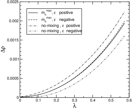
Figure 5: The variation of $\Delta\rho^{\tilde{q}}$ with $\lambda(=\lambda^{t}=\lambda^{b})$ in the $m_{h}^{\rm max}$ and no-mixing scenarios for different relative signs of $\epsilon$ and $\lambda$. $M_{\mathrm{SUSY}}=2\,\,\mathrm{TeV}$, other SUSY parameters as given in (47).

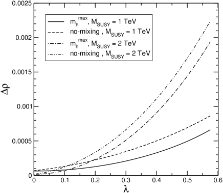
Figure 6: The variation of $\Delta\rho^{\tilde{q}}$ with $\lambda=\lambda^{t}=\lambda^{b}$ in the $m_{h}^{\rm max}$ scenario and no-mixing scenario. $M_{\mathrm{SUSY}}$ has been fixed to $1\,\,\mathrm{TeV}$ and $2\,\,\mathrm{TeV}$.

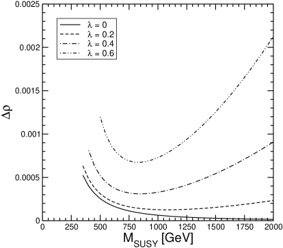
Figure 7: The variation of $\Delta\rho^{\tilde{q}}$ with $M_{\mathrm{SUSY}}$ in the $m_{h}^{\rm max}$ scenario (left panel) and no-mixing scenario (right panel), for different values of $\lambda$.

In Fig. 6 we show the dependence of $\Delta\rho^{\tilde{q}}$ on $\lambda(=\lambda^{t}=\lambda^{b})$ for both the $m_{h}^{\rm max}$ and no-mixing scenario and for two values of the SUSY mass scale, $M_{\mathrm{SUSY}}=1\,\,\mathrm{TeV}$ and $M_{\mathrm{SUSY}}=2\,\,\mathrm{TeV}$. It is clear that $\Delta\rho^{\tilde{q}}$ grows with the $\lambda$ parameter, being close to zero for $\lambda=0$ and $M_{\mathrm{SUSY}}=2\,\,\mathrm{TeV}$. One can also see that the effects on $\Delta\rho^{\tilde{q}}$ are in general larger for the no-mixing scenario (see also the results shown in Ref. [8]). For large values of $M_{\mathrm{SUSY}}$ the correction increases with increasing $\lambda$ since the splitting in the squark sector increases.

The behavior of the corrections with the SUSY mass scale is shown in Fig. 7 for different values of $\lambda$ in the $m_{h}^{\rm max}$ scenario (left panel) and in the no-mixing scenario (right panel). The region below $M_{\mathrm{SUSY}}\;\raisebox{-3.00003pt}{$\stackrel{{\scriptstyle\displaystyle<}}{{\sim}}$}\;400\,\,\mathrm{GeV}$ (depending on the scenario) implies too low and hence forbidden values for the squark masses. The curves are only for the allowed regions. For $\lambda=0$, $\Delta\rho^{\tilde{q}}$ decreases, being zero for large $M_{\mathrm{SUSY}}$ values, in agreement with the results shown in Ref. [8]. We have also found that, for $\lambda\neq 0$ and small values of $M_{\mathrm{SUSY}}$, $\Delta\rho^{\tilde{q}}$ decreases until it reaches a minimum and then increases for largest values of the SUSY scale. This increasing behavior is more pronounced for larger $\lambda$ values, reaching the level of a few per mill. The reason can be found once again the increasing mass splitting.

We also consider the possibility of choosing different values for $\lambda^{t}$ and $\lambda^{b}$. We have checked that $\Delta\rho^{\tilde{q}}$ increases with $\lambda^{t}$ and $\lambda^{b}$ independently, being smallest for $\lambda^{t}=\lambda^{b}=0$. If $\lambda^{t}$ is very different from $\lambda^{b}$, the values for $\Delta\rho^{\tilde{q}}$ can be very large. For example, for the MSSM parameters we have chosen, $\Delta\rho^{\tilde{q}}$ can be as large as $0.08$ for $\lambda^{t}=0.6,\lambda^{b}=0$. However, the large splitting between these two parameters is disfavored (see the discussion at the end of Sect. 2).

4.3 Numerical evaluation for $M_{W}$ and $\sin^{2}\theta_{\mathrm{eff}}$

Here the numerical effects of the NMFV contributions on the electroweak precision observables, $\delta M_{W}$ and $\delta\sin^{2}\theta_{\mathrm{eff}}$, are briefly analyzed. The shifts in $M_{W}$ and $\sin^{2}\theta_{\mathrm{eff}}$ have been evaluated both from the complete expressions for the scalar quark contributions, eqs. (26)-(27), and using the $\Delta\rho^{\tilde{q}}$ approximation (25). The corrections to these two observables based on (25) as a function of $\lambda(=\lambda^{t}=\lambda^{b})$ are presented in Fig. 8 with the other parameters chosen according to (47). The $m_{h}^{\rm max}$ scenario and no-mixing scenario are selected for both plots, with two values of $M_{\mathrm{SUSY}}$, as before. The induced shifts in $M_{W}$ can become as large as $0.14\,\,\mathrm{GeV}$ for the extreme case, i.e. when $M_{\mathrm{SUSY}}=2\,\,\mathrm{TeV}$, $\lambda=0.6$ and the case of no-mixing is considered. In the $m_{h}^{\rm max}$ scenario $\delta M_{W}$ is smaller, $\delta M_{W}\;\raisebox{-3.00003pt}{$\stackrel{{\scriptstyle\displaystyle<}}{{\sim}}$}\;0.05\,\,\mathrm{GeV}$, but still sizeable. Using the complete expressions (26)-(27) yields results practically indistinguishable from those shown in Fig. 8. Thus (25) is a sufficiently accurate, simple approximation for squark-mixing effects in the electroweak precision observables.

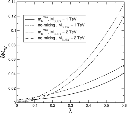
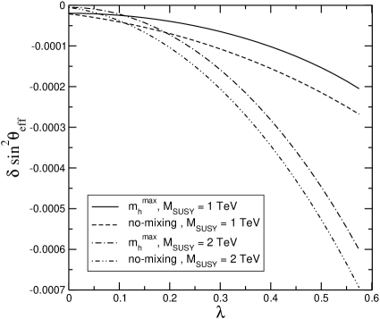
Figure 8: The variation of $\delta M_{W}$ and $\delta\sin^{2}\theta_{\mathrm{eff}}$ as a function of $\lambda=\lambda^{t}=\lambda^{b}$, for the $m_{h}^{\rm max}$ and no-mixing scenarios and different choices of $M_{\mathrm{SUSY}}$ obtained with (25). Using the complete expressions (26)-(27) yields practically indistinguishable results.

The shifts $\delta\sin^{2}\theta_{\mathrm{eff}}$, shown in the right plot of Fig. 8, can reach values up $7\times 10^{-4}$ for $M_{\mathrm{SUSY}}=2$ TeV and $\lambda=0.6$ in the no-mixing scenario, being smaller (but still sizeable) for the other scenarios chosen here.

These variations have to be compared with the current experimental uncertainties [39],

$$\Delta M_{W}^{\rm exp,today}=34\,\,\mathrm{MeV},\qquad\Delta\sin^{2}\theta_{\mathrm{eff}}^{\rm exp,today}=17\times 10^{-5}\,,$$ (48)

and the expected experimental precision for the LHC, $\Delta M_{W}=15-20\,\,\mathrm{MeV}$ [40], and at a future linear collider running on the $Z$ peak and the $WW$ threshold (GigaZ) [41, 42, 43],

$$\Delta M_{W}^{\rm exp,future}=7\,\,\mathrm{MeV},\qquad\Delta\sin^{2}\theta_{\mathrm{eff}}^{\rm exp,future}=1.3\times 10^{-5}~{}.$$ (49)

Extreme parts of the NMFV parameters (especially for $\lambda^{t}\neq\lambda^{b}$) can be excluded already with today’s precision. But even small values of $\lambda=\lambda^{t}=\lambda^{b}$ could be probed with the future precision on $\sin^{2}\theta_{\mathrm{eff}}$, provided that theoretical uncertainties will be sufficiently under control [44].

5 Conclusions

We have calculated the MSSM scalar-quark contributions to electroweak observables arising from a NMFV mixing of the third and second generation squarks. In particular, we have evaluated the lightest MSSM Higgs boson mass, the $\rho$-parameter, and the electroweak precision observables $M_{W}$ and $\sin^{2}\theta_{\mathrm{eff}}$. The analytical results have been obtained for a general $4\times 4$ mixing in the $\tilde{t}/\tilde{c}$ as well as in the $\tilde{b}/\tilde{s}$ sector. They have been included in the Fortran code FeynHiggs2.1 (see www.feynhiggs.de). The numerical analysis has been performed for a simplified model in which only the left-handed squarks receive an additional non-CKM mixing contribution.

Numerically we compared the effects of NMFV on the mass of the lightest MSSM Higgs boson in five benchmark scenarios. For small and moderate NMFV the effect is small, being at present lower than the theoretical uncertainty of $m_{h}$, $\delta m_{h}^{\rm theo}\approx 3\,\,\mathrm{GeV}$ [26].

We have presented the analytical results for the squark contribution to the $\rho$-parameter. The additional contribution can be of ${\cal O}(10^{-3})$ and can significantly depend on the relative sign of CKM and non-CKM generation mixing. Even larger contributions can be obtained if the mixing in the $\tilde{t}/\tilde{c}$ and $\tilde{b}/\tilde{s}$ sector is varied independently.

Finally we have analyzed the NMFV corrections to the electroweak precision observables $M_{W}$ and $\sin^{2}\theta_{\mathrm{eff}}$. We have shown that the effects of scalar-quark generation mixing enters essentially through $\Delta\rho$. Large parts of the parameter space can be excluded already with today’s experimental precision of these observables, and even more for the increasing precision at future colliders.

Acknowledgements

We thank T. Hahn for technical help. We thank P. Slavich and M. Vogt for helpful discussions. S.H. thanks A. Dedes, T. Hurth, S. Khalil, G. Moortgat-Pick, D. Stöckinger and G. Weiglein for interesting discussions. This work has been supported by the European Community’s Human Potential Programme under contract HPRN-CT-2000-00149 Physics at Colliders. Part of the work of S.P. has been supported by the European Union under contract No. MEIF-CT-2003-500030.

Appendix

Appendix A The Feynman rules in the MSSM with NMFV

In this section we list the Feynman rules for the various vertices used in this paper. Note that the first generation has been completely neglected and the indices have been shifted accordingly: $m_{u_{1}}$ corresponds to $m_{c}$, $m_{u_{2}}$ to $m_{t}$, $A_{1}^{u}$ to $A_{c}$, $A_{2}^{u}$ to $A_{t}$ (and analogous in the for down-type sector). The CKM matrix, $V_{\rm CKM}$, is defined as in (44). (The Feynman rules for the general case of three generation mixing can be obtained by replacing ’2’ by ’3’ in the sum and in the $R$ indices.)

A.1  2 Higgs – 2 Squarks

$\displaystyle C(h,h,\tilde{u}_{\beta},-\tilde{u}_{\alpha})=\displaystyle-\frac{\displaystyle\mathrm{i}\,e^{2}\,\sum\limits_{n=1}^{2}\left\{\begin{gathered}\left(\left(c_{2\alpha}\,M_{W}^{2}\,s_{\beta}^{2}\right)\,\left(-3+4\,s_{W}^{2}\right)+6\,c_{\alpha}^{2}\,c_{W}^{2}\,m_{u_{n}}^{2}\right)\,\left(R^{\alpha,n}_{\tilde{u}}\,(R^{\beta,n}_{\tilde{u}})^{*}\right)+\hfill\\ \left(-2\,c_{2\alpha}\,M_{W}^{2}\,s_{\beta}^{2}\,s_{W}^{2}+3\,c_{\alpha}^{2}\,c_{W}^{2}\,m_{u_{n}}^{2}\right)\,\left(2\,R^{\alpha,2+n}_{\tilde{u}}\,(R^{\beta,2+n}_{\tilde{u}})^{*}\right)\hfill\end{gathered}\right\}}{12\,c_{W}^{2}\,M_{W}^{2}\,s_{\beta}^{2}\,s_{W}^{2}}$

$\displaystyle C(h,h,\tilde{d}_{\beta},-\tilde{d}_{\alpha})=\frac{\displaystyle\mathrm{i}\,e^{2}\,\sum\limits_{n=1}^{2}\left\{\begin{gathered}\left(\left(c_{2\alpha}\,c_{\beta}^{2}\,M_{W}^{2}\right)\,\left(-3+2\,s_{W}^{2}\right)-6\,c_{W}^{2}\,s_{\alpha}^{2}\,m_{d_{n}}^{2}\right)\,\left(R^{\alpha,n}_{\tilde{d}}\,(R^{\beta,n}_{\tilde{d}})^{*}\right)-\hfill\\ \left(c_{2\alpha}\,c_{\beta}^{2}\,M_{W}^{2}\,s_{W}^{2}+3\,c_{W}^{2}\,s_{\alpha}^{2}\,m_{d_{n}}^{2}\right)\,\left(2\,R^{\alpha,2+n}_{\tilde{d}}\,(R^{\beta,2+n}_{\tilde{d}})^{*}\right)\hfill\end{gathered}\right\}}{12\,c_{\beta}^{2}\,c_{W}^{2}\,M_{W}^{2}\,s_{W}^{2}}$

$\displaystyle C(H,H,\tilde{u}_{\beta},-\tilde{u}_{\alpha})=\displaystyle-\frac{\displaystyle\mathrm{i}\,e^{2}\,\sum\limits_{n=1}^{2}\left\{\begin{gathered}\left(\left(c_{2\alpha}\,M_{W}^{2}\,s_{\beta}^{2}\right)\,\left(3-4\,s_{W}^{2}\right)+6\,c_{W}^{2}\,s_{\alpha}^{2}\,m_{u_{n}}^{2}\right)\,\left(R^{\alpha,n}_{\tilde{u}}\,(R^{\beta,n}_{\tilde{u}})^{*}\right)+\hfill\\ \left(2\,c_{2\alpha}\,M_{W}^{2}\,s_{\beta}^{2}\,s_{W}^{2}+3\,c_{W}^{2}\,s_{\alpha}^{2}\,m_{u_{n}}^{2}\right)\,\left(2\,R^{\alpha,2+n}_{\tilde{u}}\,(R^{\beta,2+n}_{\tilde{u}})^{*}\right)\hfill\end{gathered}\right\}}{12\,c_{W}^{2}\,M_{W}^{2}\,s_{\beta}^{2}\,s_{W}^{2}}$

$\displaystyle C(H,H,\tilde{d}_{\beta},-\tilde{d}_{\alpha})=\displaystyle-\frac{\displaystyle\mathrm{i}\,e^{2}\,\sum\limits_{n=1}^{2}\left\{\begin{gathered}\left(\left(c_{2\alpha}\,c_{\beta}^{2}\,M_{W}^{2}\right)\,\left(-3+2\,s_{W}^{2}\right)+6\,c_{\alpha}^{2}\,c_{W}^{2}\,m_{d_{n}}^{2}\right)\,\left(R^{\alpha,d}_{\tilde{d}}\,(R^{\beta,n}_{\tilde{d}})^{*}\right)-\hfill\\ \left(c_{2\alpha}\,c_{\beta}^{2}\,M_{W}^{2}\,s_{W}^{2}-3\,c_{\alpha}^{2}\,c_{W}^{2}\,m_{d_{n}}^{2}\right)\,\left(2\,R^{\alpha,2+n}_{\tilde{d}}\,(R^{\beta,2+n}_{\tilde{d}})^{*}\right)\hfill\end{gathered}\right\}}{12\,c_{\beta}^{2}\,c_{W}^{2}\,M_{W}^{2}\,s_{W}^{2}}$

$\displaystyle C(A,A,\tilde{u}_{\beta},-\tilde{u}_{\alpha})=\displaystyle-\frac{\displaystyle\mathrm{i}\,e^{2}\,\sum\limits_{n=1}^{2}\left\{\begin{gathered}\left(\left(c_{2\beta}\,M_{W}^{2}\,{t^{2}_{\beta}}\right)\,\left(-3+4\,s_{W}^{2}\right)+6\,c_{W}^{2}\,m_{u_{n}}^{2}\right)\,\left(R^{\alpha,n}_{\tilde{u}}\,(R^{\beta,n}_{\tilde{u}})^{*}\right)+\hfill\\ \left(-2\,c_{2\beta}\,M_{W}^{2}\,s_{W}^{2}\,{t^{2}_{\beta}}+3\,c_{W}^{2}\,m_{u_{n}}^{2}\right)\,\left(2\,R^{\alpha,2+n}_{\tilde{u}}\,(R^{\beta,2+n}_{\tilde{u}})^{*}\right)\hfill\end{gathered}\right\}}{12\,c_{W}^{2}\,M_{W}^{2}\,s_{W}^{2}\,{t^{2}_{\beta}}}$

$\displaystyle C(A,A,\tilde{d}_{\beta},-\tilde{d}_{\alpha})=\displaystyle-\frac{\displaystyle\mathrm{i}\,e^{2}\,\sum\limits_{n=1}^{2}\left\{\begin{gathered}\left(\left(c_{2\beta}\,M_{W}^{2}\right)\,\left(3-2\,s_{W}^{2}\right)+6\,c_{W}^{2}\,{t^{2}_{\beta}}\,m_{d_{n}}^{2}\right)\,\left(R^{\alpha,n}_{\tilde{d}}\,(R^{\beta,n}_{\tilde{d}})^{*}\right)+\hfill\\ \left(c_{2\beta}\,M_{W}^{2}\,s_{W}^{2}+3\,c_{W}^{2}\,{t^{2}_{\beta}}\,m_{d_{n}}^{2}\right)\,\left(2\,R^{\alpha,2+n}_{\tilde{d}}\,(R^{\beta,2+n}_{\tilde{d}})^{*}\right)\hfill\end{gathered}\right\}}{12\,c_{W}^{2}\,M_{W}^{2}\,s_{W}^{2}}$

$\displaystyle C(h,H,\tilde{u}_{\beta},-\tilde{u}_{\alpha})=\displaystyle-\frac{\displaystyle\mathrm{i}\,e^{2}\,s_{2\alpha}\,\sum\limits_{n=1}^{2}\left\{\begin{gathered}\left(\left(M_{W}^{2}\,s_{\beta}^{2}\right)\,\left(-3+4\,s_{W}^{2}\right)+3\,c_{W}^{2}\,m_{u_{n}}^{2}\right)\,\left(R^{\alpha,n}_{\tilde{u}}\,(R^{\beta,n}_{\tilde{u}})^{*}\right)+\hfill\\ \left(-4\,M_{W}^{2}\,s_{\beta}^{2}\,s_{W}^{2}+3\,c_{W}^{2}\,m_{u_{n}}^{2}\right)\,\left(R^{\alpha,2+n}_{\tilde{u}}\,(R^{\beta,2+n}_{\tilde{u}})^{*}\right)\hfill\end{gathered}\right\}}{12\,c_{W}^{2}\,M_{W}^{2}\,s_{\beta}^{2}\,s_{W}^{2}}$

$\displaystyle C(h,H,\tilde{d}_{\beta},-\tilde{d}_{\alpha})=\frac{\displaystyle\mathrm{i}\,e^{2}\,s_{2\alpha}\,\sum\limits_{n=1}^{2}\left\{\begin{gathered}\left(\left(c_{\beta}^{2}\,M_{W}^{2}\right)\,\left(-3+2\,s_{W}^{2}\right)+3\,c_{W}^{2}\,m_{d_{n}}^{2}\right)\,\left(R^{\alpha,n}_{\tilde{d}}\,(R^{\beta,n}_{\tilde{d}})^{*}\right)+\hfill\\ \left(-2\,c_{\beta}^{2}\,M_{W}^{2}\,s_{W}^{2}+3\,c_{W}^{2}\,m_{d_{n}}^{2}\right)\,\left(R^{\alpha,2+n}_{\tilde{d}}\,(R^{\beta,2+n}_{\tilde{d}})^{*}\right)\hfill\end{gathered}\right\}}{12\,c_{\beta}^{2}\,c_{W}^{2}\,M_{W}^{2}\,s_{W}^{2}}$

A.2  2 Squarks – 2 Gauge Bosons

$\displaystyle C(\tilde{u}_{\alpha},-\tilde{u}_{\beta},Z,Z)=\frac{\displaystyle\mathrm{i}\,e^{2}}{18\,c_{W}^{2}\,s_{W}^{2}}\,\sum\limits_{n=1}^{2}{\left(3-4\,s_{W}^{2}\right)}^{2}\,R^{\beta,n}_{\tilde{u}}\,(R^{\alpha,n}_{\tilde{u}})^{*}+16\,{s_{W}}^{4}\,R^{\beta,2+n}_{\tilde{u}}\,(R^{\alpha,2+n}_{\tilde{u}})^{*}$

$\displaystyle C(\tilde{d}_{\alpha},-\tilde{d}_{\beta},Z,Z)=\frac{\displaystyle\mathrm{i}\,e^{2}}{18\,c_{W}^{2}\,s_{W}^{2}}\,\sum\limits_{n=1}^{2}{\left(3-2\,s_{W}^{2}\right)}^{2}\,R^{\beta,n}_{\tilde{d}}\,(R^{\alpha,n}_{\tilde{d}})^{*}+4\,{s_{W}}^{4}\,R^{\beta,2+n}_{\tilde{d}}\,(R^{\alpha,2+n}_{\tilde{d}})^{*}$

$\displaystyle C(\tilde{d}_{\beta},-\tilde{u}_{\alpha},Z,-W^{-})=\displaystyle-\displaystyle\mathrm{i}{\,e^{2}\,\sum\limits_{n,m=1}^{2}V^{n,m}_{\text{\rm CKM}}\,(R^{\beta,m}_{\tilde{d}})^{*}\,R^{\alpha,n}_{\tilde{u}}}{3\,{\sqrt{2}}\,c_{W}}$

$\displaystyle C(\tilde{u}_{\alpha},-\tilde{u}_{\beta},W^{-},-W^{-})=\frac{\displaystyle\mathrm{i}\,e^{2}}{2\,s_{W}^{2}}\,\sum\limits_{n=1}^{2}R^{\beta,n}_{\tilde{u}}\,(R^{\alpha,n}_{\tilde{u}})^{*}$

$\displaystyle C(\tilde{d}_{\alpha},-\tilde{d}_{\beta},W^{-},-W^{-})=\frac{\displaystyle\mathrm{i}\,e^{2}}{2\,s_{W}^{2}}\,\sum\limits_{n=1}^{2}R^{\beta,n}_{\tilde{d}}\,(R^{\alpha,n}_{\tilde{d}})^{*}$

A.3  2 Squarks – Gauge Boson

$\displaystyle C(\tilde{u}_{\alpha},-\tilde{u}_{\beta},Z)=\frac{\displaystyle\mathrm{i}\,e}{6\,c_{W}\,s_{W}}\,\sum\limits_{n=1}^{2}\left(-3+4\,s_{W}^{2}\right)\,\left(R^{\beta,n}_{\tilde{u}}\,(R^{\alpha,n}_{\tilde{u}})^{*}\right)+4\,s_{W}^{2}\,R^{\beta,2+n}_{\tilde{u}}\,(R^{\alpha,2+n}_{\tilde{u}})^{*}$

$\displaystyle C(\tilde{d}_{\alpha},-\tilde{d}_{\beta},Z)=\displaystyle-\frac{\displaystyle\mathrm{i}\,e}{6\,c_{W}\,s_{W}}\,\sum\limits_{n=1}^{2}\left(-3+2\,s_{W}^{2}\right)\,\left(R^{\beta,n}_{\tilde{d}}\,(R^{\alpha,n}_{\tilde{d}})^{*}\right)+2\,s_{W}^{2}\,R^{\beta,2+n}_{\tilde{d}}\,(R^{\alpha,2+n}_{\tilde{d}})^{*}$

$\displaystyle C(\tilde{u}_{\alpha},-\tilde{d}_{\beta},W^{-})=\displaystyle-\frac{\displaystyle\mathrm{i}\,e}{{\sqrt{2}}\,s_{W}}\,\sum\limits_{n,m=1}^{2}(V^{n,m}_{\text{\rm CKM}})^{*}\,R^{\beta,m}_{\tilde{d}}\,(R^{\alpha,n}_{\tilde{u}})^{*}$

$\displaystyle C(\tilde{d}_{\beta},-\tilde{u}_{\alpha},-W^{-})=\displaystyle-\frac{\displaystyle\mathrm{i}\,e}{{\sqrt{2}}\,s_{W}}\,\sum\limits_{n,m=1}^{2}V^{n,m}_{\text{\rm CKM}}\,(R^{\beta,m}_{\tilde{d}})^{*}\,R^{\alpha,n}_{\tilde{u}}$

A.4  Higgs – 2 Squarks

$\displaystyle C(h,\tilde{u}_{\alpha},-\tilde{u}_{\beta})=\displaystyle-\frac{\displaystyle\mathrm{i}\,e\,\sum\limits_{n=1}^{2}\left\{\begin{gathered}\left(\left(\left(M_{W}\,M_{Z}\,s_{\alpha+\beta}\,s_{\beta}\right)\,\left(-3+4\,s_{W}^{2}\right)+6\,c_{\alpha}\,c_{W}\,m_{u_{n}}^{2}\right)\,R^{\beta,n}_{\tilde{u}}+\left(c_{\alpha}\,A^{u}_{n}+\right.\right.\\ \left.\left.s_{\alpha}\,\mu^{*}\right)\left(3\,c_{W}\,m_{u_{n}}\,R^{\beta,2+n}_{\tilde{u}}\right)\right)\,(R^{\alpha,n}_{\tilde{u}})^{*}+\left(\left(\mu\,s_{\alpha}+c_{\alpha}\,A^{u*}_{n}\right)\,\left(3\,c_{W}\,m_{u_{n}}\,R^{\beta,n}_{\tilde{u}}\right)\right.\\ \left.-4\,M_{W}\,M_{Z}\,s_{\alpha+\beta}\,s_{\beta}\,s_{W}^{2}\,R^{\beta,2+n}_{\tilde{u}}+6\,c_{\alpha}\,c_{W}\,m_{u_{n}}^{2}\,R^{\beta,2+n}_{\tilde{u}}\right)\,(R^{\alpha,2+n}_{\tilde{u}})^{*}\hfill\end{gathered}\right\}}{6\,c_{W}\,M_{W}\,s_{\beta}\,s_{W}}$

$\displaystyle C(h,\tilde{d}_{\alpha},-\tilde{d}_{\beta})=\frac{\displaystyle\mathrm{i}\,e\,\sum\limits_{n=1}^{2}\left\{\begin{gathered}\left(\left(\left(c_{\beta}\,M_{W}\,M_{Z}\,s_{\alpha+\beta}\right)\,\left(-3+2\,s_{W}^{2}\right)+6\,c_{W}\,s_{\alpha}\,m_{d_{n}}^{2}\right)\,R^{\beta,n}_{\tilde{d}}+\left(s_{\alpha}\,A^{d}_{n}+c_{\alpha}\,\mu^{*}\right)\right.\\ \left.\left(3\,c_{W}\,m_{d_{n}}\,R^{\beta,2+n}_{\tilde{d}}\right)\right)\,(R^{\alpha,n}_{\tilde{d}})^{*}+\left(\left(c_{\alpha}\,\mu+s_{\alpha}\,A^{d*}_{n}\right)\,\left(3\,c_{W}\,m_{d_{n}}\,R^{\beta,n}_{\tilde{d}}\right)-\right.\\ \left.2\,c_{\beta}\,M_{W}\,M_{Z}\,s_{\alpha+\beta}\,s_{W}^{2}\,R^{\beta,2+n}_{\tilde{d}}+6\,c_{W}\,s_{\alpha}\,m_{d_{n}}^{2}\,R^{\beta,2+n}_{\tilde{d}}\right)\,(R^{\alpha,2+n}_{\tilde{d}})^{*}\hfill\end{gathered}\right\}}{6\,c_{\beta}\,c_{W}\,M_{W}\,s_{W}}$

$\displaystyle C(A,\tilde{u}_{\alpha},-\tilde{u}_{\beta})=\displaystyle-\frac{\displaystyle e\,\sum\limits_{n=1}^{2}\left(-\left(A^{u}_{n}+t_{\beta}\,\mu^{*}\right)\,\left(R^{\beta,2+n}_{\tilde{u}}\,(R^{\alpha,n}_{\tilde{u}})^{*}\right)+\left(A^{u*}_{n}+\mu\,t_{\beta}\right)\,\left(R^{\beta,n}_{\tilde{u}}\,(R^{\alpha,2+n}_{\tilde{u}})^{*}\right)\right)\,m_{u_{n}}}{2\,M_{W}\,s_{W}\,t_{\beta}}$

$\displaystyle C(A,\tilde{d}_{\alpha},-\tilde{d}_{\beta})=\displaystyle-\frac{\displaystyle e\,\sum\limits_{n=1}^{2}\left(-\left(\mu^{*}+t_{\beta}\,A^{d}_{n}\right)\,\left(R^{\beta,2+n}_{\tilde{d}}\,(R^{\alpha,n}_{\tilde{d}})^{*}\right)+\left(\mu+t_{\beta}\,A^{d*}_{n}\right)\,\left(R^{\beta,n}_{\tilde{d}}\,(R^{\alpha,2+n}_{\tilde{d}})^{*}\right)\right)\,m_{d_{n}}}{2\,M_{W}\,s_{W}}$

$\displaystyle C(H,\tilde{u}_{\alpha},-\tilde{u}_{\beta})=\displaystyle-\frac{\displaystyle\mathrm{i}\,e\,\sum\limits_{n=1}^{2}\left\{\begin{gathered}\left(\left(\left(c_{\alpha+\beta}\,M_{W}\,M_{Z}\,s_{\beta}\right)\,\left(3-4\,s_{W}^{2}\right)+6\,c_{W}\,s_{\alpha}\,m_{u_{n}}^{2}\right)\,R^{\beta,n}_{\tilde{u}}+\left(s_{\alpha}\,A^{u}_{n}-c_{\alpha}\,\mu^{*}\right)\right.\\ \left.\left(3\,c_{W}\,m_{u_{n}}\,R^{\beta,2+n}_{\tilde{u}}\right)\right)\,(R^{\alpha,n}_{\tilde{u}})^{*}+\left(\left(-c_{\alpha}\,\mu+s_{\alpha}\,A^{u*}_{n}\right)\,\left(3\,c_{W}\,m_{u_{n}}\,R^{\beta,n}_{\tilde{u}}\right)+\right.\\ \left.4\,c_{\alpha+\beta}\,M_{W}\,M_{Z}\,s_{\beta}\,s_{W}^{2}\,R^{\beta,2+n}_{\tilde{u}}+6\,c_{W}\,s_{\alpha}\,m_{u_{n}}^{2}\,R^{\beta,2+n}_{\tilde{u}}\right)\,(R^{\alpha,2+n}_{\tilde{u}})^{*}\hfill\end{gathered}\right\}}{6\,c_{W}\,M_{W}\,s_{\beta}\,s_{W}}$

$\displaystyle C(H,\tilde{d}_{\alpha},-\tilde{d}_{\beta})=\displaystyle-\frac{\displaystyle\mathrm{i}\,e\,\sum\limits_{n=1}^{2}\left\{\begin{gathered}\left(\left(\left(c_{\alpha+\beta}\,c_{\beta}\,M_{W}\,M_{Z}\right)\,\left(-3+2\,s_{W}^{2}\right)+6\,c_{\alpha}\,c_{W}\,m_{d_{n}}^{2}\right)\,R^{\beta,n}_{\tilde{d}}+\left(c_{\alpha}\,A^{d}_{n}-\right.\right.\\ \left.\left.s_{\alpha}\,\mu^{*}\right)\left(3\,c_{W}\,m_{d_{n}}\,R^{\beta,2+n}_{\tilde{d}}\right)\right)\,(R^{\alpha,n}_{\tilde{d}})^{*}+\left(\left(-\mu\,s_{\alpha}+c_{\alpha}\,A^{d*}_{n}\right)\,\left(3\,c_{W}\,m_{d_{n}}\,R^{\beta,n}_{\tilde{d}}\right)\right.\\ \left.-2\,c_{\alpha+\beta}\,c_{\beta}\,M_{W}\,M_{Z}\,s_{W}^{2}\,R^{\beta,2+n}_{\tilde{d}}+6\,c_{\alpha}\,c_{W}\,m_{d_{n}}^{2}\,R^{\beta,2+n}_{\tilde{d}}\right)\,(R^{\alpha,2+n}_{\tilde{d}})^{*}\hfill\end{gathered}\right\}}{6\,c_{\beta}\,c_{W}\,M_{W}\,s_{W}}$

References

-
[1]
H.P. Nilles,
Phys. Rep. 110 (1984) 1;
H.E. Haber and G.L. Kane, Phys. Rep. 117, (1985) 75;
R. Barbieri, Riv. Nuovo Cim. 11, (1988) 1. - [2] K. Hagiwara et al. [Particle Data Group], Phys. Rev. D 66 (2002) 010001.
- [3] J. Gunion, H. Haber, G. Kane and S. Dawson, The Higgs Hunter’s Guide, Addison-Wesley, 1990.
- [4] ALEPH, DELPHI, L3 and OPAL Collaborations, and the LEP Higgs working group, Phys. Lett. B 565 (2003) 61, hep-ex/0306033; hep-ex/0107030; hep-ex/0107031; LHWG Note 2001-4, see: lephiggs.web.cern.ch/LEPHIGGS/papers/ .
- [5] M. Veltman, Nucl. Phys. B 123 (1977) 89.
-
[6]
R. Barbieri and L. Maiani,
Nucl. Phys. B 224 (1983) 32;
C. S. Lim, T. Inami and N. Sakai, Phys. Rev. D 29 (1984) 1488;
E. Eliasson, Phys. Lett. B 147 (1984) 65;
Z. Hioki, Prog. Theo. Phys. 73 (1985) 1283;
J. A. Grifols and J. Sola, Nucl. Phys. B 253 (1985) 47;
B. Lynn, M. Peskin and R. Stuart, CERN Report 86-02, p. 90;
R. Barbieri, M. Frigeni, F. Giuliani and H.E. Haber, Nucl. Phys. B 341 (1990) 309;
M. Drees and K. Hagiwara, Phys. Rev. D 42 (1990) 1709. -
[7]
M. Drees, K. Hagiwara and A. Yamada,
Phys. Rev. D 45 (1992) 1725;
P. Chankowski, A. Dabelstein, W. Hollik, W. Mösle, S. Pokorski and J. Rosiek, Nucl. Phys. B 417 (1994) 101;
D. Garcia and J. Solà, Mod. Phys. Lett. A 9 (1994) 211.
A. Dabelstein, W. Hollik, W. Mösle, hep-ph/9506251, in Proceedings of the Ringberg Workshop on Perspectives for electroweak interactions in collisions, Ringberg 1995, ed. B. Kniehl [QCD162:E4:1995];
W. de Boer, A. Dabelstein, W. Hollik, W. Mösle, U. Schwickerath, Z. Phys. C75 (1997) 627, hep-ph/9607286; hep-ph/9609209;
D. Pierce, J. Bagger, T. Matchev, R. Zhang, Nucl. Phys. B 491 (1997) 3, hep-ph/9606211. - [8] A. Djouadi, P. Gambino, S. Heinemeyer, W. Hollik, C. Jünger and G. Weiglein, Phys. Rev. Lett. 78 (1997) 3626, hep-ph/9612363; Phys. Rev. D 57 (1998) 4179, hep-ph/9710438.
-
[9]
S. Heinemeyer, PhD thesis,
see www-itp.physik.uni-karlsruhe.de/prep/phd/;
G. Weiglein, hep-ph/9901317;
S. Heinemeyer, W. Hollik and G. Weiglein, in preparation. - [10] S. Heinemeyer and G. Weiglein, JHEP 0210 (2002) 072, hep-ph/0209305; hep-ph/0301062.
- [11] J. Aguilar-Saavedra et al., TESLA TDR Part 3: “Physics at an Linear Collider”, hep-ph/0106315, see: tesla.desy.de/tdr/ .
- [12] T. Abe et al. [American Linear Collider Working Group], “Linear collider physics resource book for Snowmass 2001”, hep-ex/0106055; hep-ex/0106056.
- [13] K. Abe et al. [ACFA Linear Collider Working Group], “Particle physics experiments at JLC”, hep-ph/0109166, see: lcdev.kek.jp/RMdraft/ .
- [14] P. Chankowski, S. Pokorski and J. Rosiek, Phys. Lett. B 286 (1992) 307; Nucl. Phys. B 423 (1994) 423, hep-ph/9303309.
- [15] A. Dabelstein, Nucl. Phys. B 456 (1995) 25, hep-ph/9503443; Z. Phys. C 67 (1995) 495, hep-ph/9409375.
-
[16]
R. Hempfling and A. Hoang,
Phys. Lett. B 331 (1994) 99,
hep-ph/9401219;
R. Zhang, Phys. Lett. B 447 (1999) 89, hep-ph/9808299;
J. Espinosa and R. Zhang, Nucl. Phys. B 586 (2000) 3, hep-ph/0003246. - [17] G. Degrassi, P. Slavich and F. Zwirner, Nucl. Phys. B 611 (2001) 403, hep-ph/0105096.
-
[18]
A. Brignole, G. Degrassi, P. Slavich and F. Zwirner,
Nucl. Phys. B 631 (2002) 195,
hep-ph/0112177;
Nucl. Phys. B 643 (2002) 79,
hep-ph/0206101;
A. Dedes, G. Degrassi and P. Slavich, Nucl. Phys. B 672 (2003) 144, hep-ph/0305127. - [19] S. Martin, hep-ph/0211366; Phys. Rev. D 65 (2002) 116003, hep-ph/0111209; Phys. Rev. D 66 (2002) 096001, hep-ph/0206136.
-
[20]
M. Carena, J. Espinosa, M. Quirós and C. Wagner,
Phys. Lett. B 355 (1995) 209,
hep-ph/9504316;
M. Carena, M. Quirós and C. Wagner, Nucl. Phys. B 461 (1996) 407, hep-ph/9508343;
H. Haber, R. Hempfling and A. Hoang, Z. Phys. C 75 (1997) 539, hep-ph/9609331. - [21] S. Heinemeyer, W. Hollik and G. Weiglein, Phys. Rev. D 58 (1998) 091701, hep-ph/9803277; Phys. Lett. B 440 (1998) 296, hep-ph/9807423.
- [22] S. Heinemeyer, W. Hollik and G. Weiglein, Eur. Phys. J. C 9 (1999) 343, hep-ph/9812472.
- [23] S. Heinemeyer, W. Hollik and G. Weiglein, Phys. Lett. B 455 (1999) 179, hep-ph/9903404.
- [24] M. Carena, H. Haber, S. Heinemeyer, W. Hollik, C. Wagner and G. Weiglein, Nucl. Phys. B 580 (2000) 29, hep-ph/0001002.
-
[25]
S. Heinemeyer, W. Hollik and G. Weiglein,
hep-ph/9910283;
J. Espinosa and R. Zhang, JHEP 0003 (2000) 026, hep-ph/9912236. - [26] G. Degrassi, S. Heinemeyer, W. Hollik, P. Slavich and G. Weiglein, Eur. Phys. J. C 28 (2003) 133, hep-ph/0212020.
-
[27]
J. Guasch and J. Sola,
Nucl. Phys. B 562 (1999) 3,
hep-ph/9906268;
S. Bejar, F. Dilme, J. Guasch and J. Sola, hep-ph/0402188. -
[28]
A. Curiel, M. Herrero and D. Temes,
Phys. Rev. D 67 (2003) 075008,
hep-ph/0210335;
A. Curiel, M. Herrero, W. Hollik, F. Merz and S. Peñaranda, Phys. Rev. D 69 (2004) 075009, hep-ph/0312135. - [29] P. Brax and C. Savoy, Nucl. Phys. B 447 (1995) 227, hep-ph/9503306.
-
[30]
K. Hikasa and M. Kobayashi,
Phys. Rev. D 36 (1987) 724;
F. Gabbiani and A. Masiero, Nucl. Phys. B 322 (1989) 235. - [31] F. Gabbiani, E. Gabrielli, A. Masiero and L. Silvestrini, Nucl. Phys. B 477 (1996) 321, hep-ph/9604387.
- [32] M. Misiak, S. Pokorski and J. Rosiek, Adv. Ser. Direct. High Energy Phys. 15 (1998) 795, hep-ph/9703442.
- [33] P. Ball, S. Khalil and E. Kou, hep-ph/0311361.
-
[34]
T. Besmer, C. Greub and T. Hurth,
Nucl. Phys. B 609 (2001) 359,
hep-ph/0105292;
F. Borzumati, C. Greub, T. Hurth and D. Wyler, Phys. Rev. D 62 (2000) 075005, hep-ph/9911245. -
[35]
J. Küblbeck, M. Böhm and A. Denner,
Comp. Phys. Comm. 60 (1990) 165;
T. Hahn and M. Perez-Victoria, Comput. Phys. Commun. 118 (1999) 153, hep-ph/9807565;
T. Hahn, Nucl. Phys. Proc. Suppl. 89 (2000) 231, hep-ph/0005029; Comput. Phys. Commun. 140 (2001) 418, hep-ph/0012260.
The program is available via www.feynarts.de . - [36] T. Hahn and C. Schappacher, Comput. Phys. Commun. 143 (2002) 54, hep-ph/0105349.
-
[37]
S. Heinemeyer, W. Hollik and G. Weiglein, Comp. Phys. Comm. 124 2000 76,
hep-ph/9812320;
hep-ph/0002213;
M. Frank, S. Heinemeyer, W. Hollik and G. Weiglein, hep-ph/0202166;
T. Hahn, S. Heinemeyer, W. Hollik and G. Weiglein, in preparation.
The code is accessible via www.feynhiggs.de. - [38] M. Carena, S. Heinemeyer, C. Wagner and G. Weiglein, Eur. Phys. J. C 26 (2003) 601, hep-ph/0202167.
-
[39]
The LEP Collaborations ALEPH, DELPHI, L3, OPAL, the LEP Electroweak
Working Group, the SLD Electroweak and Heavy Flavour Working Groups,
A Combination of Preliminary Electroweak Measurements and
Constraints on the Standard Model, hep-ex/0312023;
M. Grünewald, hep-ex/0304023, in Proceedings of the Workshop on Electroweak precision data and the Higgs mass, DESY Zeuthen 2003, eds. S. Dittmaier and K. Mönig, DESY-PROC-2003-1. - [40] S. Haywood et al., Report of the Electroweak Physics Working Group of the “1999 CERN Workshop on SM physics (and more) at the LHC”, hep-ph/0003275.
- [41] R. Hawkings and K. Mönig, EPJdirect C 8 (1999) 1, hep-ex/9910022.
-
[42]
S. Heinemeyer, T. Mannel and G. Weiglein,
hep-ph/9909538;
J. Erler, S. Heinemeyer, W. Hollik, G. Weiglein and P. Zerwas, Phys. Lett. B 486 (2000) 125, hep-ph/0005024;
J. Erler and S. Heinemeyer, hep-ph/0102083. - [43] U. Baur, R. Clare, J. Erler, S. Heinemeyer, D. Wackeroth, G. Weiglein and D. Wood, contribution to the P1-WG1 report of the workshop “The Future of Particle Physics”, Snowmass, Colorado, USA, July 2001, hep-ph/0111314.
-
[44]
S. Heinemeyer and G. Weiglein,
hep-ph/0307177, in
Proceedings of the Workshop on
Electroweak precision data and the Higgs mass,
DESY Zeuthen 2003,
eds. S. Dittmaier and K. Mönig,
DESY-PROC-2003-1;
S. Heinemeyer, hep-ph/0406245, to appear in the proceedings of Loops & Legs in Quantum Field Theory 2004, Zinnowitz, Germany, April 2004.