Alberta Thy 04-04 Heavy-to-light decays with a two-loop accuracy

Abstract

We present a determination of a new class of three-loop Feynman diagrams describing heavy-to-light transitions. We apply it to find the ${\cal O}\!\left(\alpha_{s}^{2}\right)$ corrections to the top quark decay $t\to bW$ and to the distribution of lepton invariant mass in the semileptonic $b$ quark decay $b\to ul\nu$. We also confirm the previously determined total rate of that process as well as the ${\cal O}\!\left(\alpha^{2}\right)$ corrections to the muon lifetime.

The determination of higher order corrections in perturbative quantum field theory is notoriously difficult, and with the general tendency towards precision measurements in particle physics, each newly-won class of perturbative integrals expands the possibilities for phenomenological analyses. For instance, quantum corrections to decays of neutral particles, such as a virtual photon or a $Z$ boson into hadrons, are known to sixth order in perturbation theory, ${\cal O}\!\left(\alpha_{s}^{3}\right)$, and even some ${\cal O}\!\left(\alpha_{s}^{4}\right)$ effects have been studied. Those results have been very useful in determining a variety of Standard Model parameters such as the $Z$ boson properties, the strong coupling constant, and the running of the electromagnetic coupling constant Steinhauser (2002).

Much less is known about radiative corrections to processes with a charged particle in the initial state. Only relatively recently have first results been obtained in fourth order perturbation theory, ${\cal O}\!\left(\alpha_{s}^{2}\right)$ and ${\cal O}\!\left(\alpha^{2}\right)$, primarily for total decay rates. The technical challenge in such calculations is the presence of massive propagators. For example, consider the muon decay. Since the muon is charged, it can emit photons, and the resulting amplitudes will involve propagators of a virtual muon. Its mass sets the energy scale of the process and cannot be treated as a small parameter.

The presence of massive propagators is an obstacle in evaluating the multi-loop diagrams required by precise measurements of heavy quark and lepton decays. So far, genuine ${\cal O}\!\left(\alpha_{s}^{2}\right)$ corrections to heavy quark decays are known only for semileptonic processes, $Q\to ql\nu(gg)$, and only for some kinematic cases. One approach that has been successful consists in expanding Feynman diagrams around the zero recoil limit: when the quark $q$ remains at rest with respect to $Q$. The kinematics of semileptonic decays can be represented by a triangle, since the invariant mass of the leptons together with the mass of the final state quark $q$ cannot exceed the mass of the decaying quark. This is depicted in Fig. 1.

Figure 1: Kinematical boundaries of the semileptonic decays $Q\to q+\mbox{leptons}$. The solid arrow shows the expansion presented in this paper. Previously known expansions are indicated with dotted arrows.

The diagonal boundary corresponds to the zero recoil limit, in which the ${\cal O}\!\left(\alpha_{s}^{2}\right)$ effects are known Czarnecki (1996); Czarnecki and Melnikov (1997); Franzkowski and Tausk (1998). Also shown are the starting points of previously studied expansions. Those results have helped improve the knowledge of the $b$ quark lifetime and the determination of the CKM matrix element $V_{cb}$.

However, the expansion around zero recoil converges slowly near the origin in Fig. 1, that is, when both the quark $q$ and the lepton pair are light; in this case computations become prohibitively expensive. Two other approaches have been used in such cases. First, for the phenomenologically important decays $\mu\to e\nu\bar{\nu}$ and $b\to ul\nu$, the total lifetimes have been determined in van Ritbergen and Stuart (1999); van Ritbergen (1999) by analytically calculating imaginary parts of four-loop diagrams. That heroic effort is difficult to extend, for example, to differential distributions. The other approach consists in expanding diagrams in an artificial parameter, for example the ratio of muon masses outside and inside loops, and using Padé approximants to sum the expansion for the physical value of this parameter. This approach was used to check the muon and $b\to u$ results Steinhauser and Seidensticker (1999); Chetyrkin et al. (1999). It yields results scattered around the exact values which are often sufficient for applications. The drawback of this method is that it is very difficult to estimate the errors reliably.

The purpose of this study is to extend the method of expansions beyond the zero recoil limit. We start directly at the origin of Fig. 1, which corresponds to the kinematics of a top quark decay into a massless $b$ quark and a massless $W$ boson. We then treat the $W$ mass as a small perturbation and compute several terms of the resulting expansion. We stop when we can smoothly match to the previously obtained expansion around the case of the $W$ boson equally heavy as the decaying quark Czarnecki and Melnikov (2002). The physical top quark decay corresponds to a specific value of the $W$ mass, but in the more general decay $Q\to q+\mbox{leptons}$, the term “$W$ mass” refers to the invariant mass of the lepton pair, and it is in this context that we can relate $t\rightarrow bW$ to $b\rightarrow ul\nu$ and $\mu\rightarrow e\nu\overline{\nu}$.

This is the first time that exact results are available in this limit and we can now address a number of interesting problems. We obtain an accurate value of the ${\cal O}\!\left(\alpha_{s}^{2}\right)$ correction to the top quark lifetime. The combination of our results with the expansion around the heavy $W$ case allows us to give a complete description of the differential distribution of $b\to ul\nu$ decay in the invariant mass of leptons, and thus improves the theoretical description of this decay, important for the determination of $V_{ub}$. We also check the muon and $b\to u$ lifetime corrections with a relative error of about $2\times 10^{-4}$. In the future, the same method can be employed to improve perturbative corrections to mixing processes such us $B_{d}\leftrightarrow\overline{B}_{d}$ and $B_{s}\leftrightarrow\overline{B}_{s}$.

In Fig. 2 we show three examples of the diagrams that we have to consider in order to calculate $t\rightarrow bW$ at ${\cal O}\!\left(\alpha_{s}^{2}\right)$. We use the optical theorem to connect the imaginary parts of such diagrams with contributions to the decay. Note that we customarily speak about two-loop corrections when what we actually need to compute are the imaginary parts of three-loop diagrams. The various cuts correspond to two-loop virtual corrections or emissions of one or two real quanta.

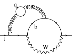
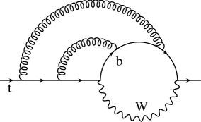
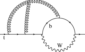
(a)	(b)	(c)

Figure 2: Examples of diagrams whose cuts contribute to the $\mathcal{O}(\alpha_{s}^{2})$ decay rate for $t\rightarrow bW$: (a) light or heavy quarks; (b) abelian; (c) non-abelian.

With $m_{b}=0$, there are two scales in the problem: $m_{t}$ and $m_{W}$. We define an expansion parameter $\omega=m_{W}^{2}/m_{t}^{2}$ so that the two scales can be expressed as hard and soft (${\cal O}\!\left(1\right)$ and ${\cal O}\!\left(\sqrt{\omega}\right)$, using $m_{t}$ as the unit of energy). Contributions arising from these two scales are identified using asymptotic expansions so that we must consider two regions. In the first region, all the loop momenta are hard and the $W$ propagator can be expanded as a series, in powers of $\omega$, of massless propagators. In the second region, the gluon momenta are hard but the loop momentum flowing through the $W$ is soft. In this region, the diagrams factor into a product of a two-loop self-energy type integral and a one-loop vacuum bubble integral with a scale of $m_{W}$. The leading contribution from this second region is ${\cal O}\!\left(\omega^{2}\right)$, and the interplay between the two regions gives rise to terms with a large logarithm $\ln\omega$.

All scalar integrals arising in the problem can be expressed in terms of $9$ basic topologies. We use differential-algebraic identities to reduce all loop integrals in both regions to a combination of $24$ master integrals. The resulting large linear systems can be solved in a few ways. In the traditional method Tkachov (1981), one inspects the structure of the identities and rearranges them manually into the form of recurrence relations for an efficient iterative solution of the system. This “by inspection” method has proven to be very successful in numerous applications (e.g., Broadhurst (1992); van Ritbergen and Stuart (1999); van Ritbergen (1999); Czarnecki and Melnikov (2002)) but it requires much human work to implement. Conversely, a straightforward solution of the linear system is much more expensive computationally and was first achieved only recently Laporta (2000). In our calculation csc we used the traditional approach (programmed in FORM Vermaseren (2000)) as well as a modified version of the new algorithm for which we implemented a dedicated computer algebra system. In both cases we independently obtained identical results which serve as a check of correctness but also enable us to compare these two methods. Details of the implementation of both methods and the evaluation of master integrals will be presented in a forthcoming technical paper.

The final result for the top quark decay width can be written as

$$\Gamma(t\rightarrow bW)=\Gamma_{0}\left[X_{0}+\frac{\alpha_{s}}{\pi}X_{1}+\left(\frac{\alpha_{s}}{\pi}\right)^{2}X_{2}\right],\qquad\Gamma_{0}\equiv\frac{G_{F}m_{t}^{3}\left|V_{tb}\right|^{2}}{8\sqrt{2}\pi}\ .$$ (1)

Throughout this paper, we use $\alpha_{s}\equiv\alpha_{s}^{\overline{MS}}(\mu)$, where $\mu$ is the pole mass of the decaying quark. The tree-level and ${\cal O}\!\left(\alpha_{s}\right)$ coefficients are already known analytically Jezabek and Kuhn (1989),

$$X_{0} = 1-3\omega^{2}+2\omega^{3}\ ,$$ (2)

$$X_{1} = C_{F}\left[\left(\frac{5}{4}-\frac{\pi^{2}}{3}\right)+\frac{3}{2}\omega+\omega^{2}\left(\pi^{2}-6+\frac{3}{2}L\right)+{\cal O}\!\left(\omega^{3}L\right)\right],\qquad L\equiv\ln\omega.$$ (3)

The ${\cal O}\!\left(\alpha_{s}^{2}\right)$ result can be subdivided into four gauge-invariant pieces,

$$X_{2}=C_{F}\left(T_{R}N_{L}X_{L}+T_{R}N_{H}X_{H}+C_{F}X_{A}+C_{A}X_{NA}\right)\ ,$$ (4)

where $C_{F}=4/3$, $C_{A}=3$, and $T_{R}=1/2$ are the usual SU(3) color factors and $N_{L}$ and $N_{H}$ denote the number of light $(m_{q}=0)$ and heavy $(m_{q}=m_{t})$ quark species. For the coefficients $X_{L}$, $X_{H}$, $X_{A}$, and $X_{NA}$, we have obtained a series to at least $\omega^{5}$, of which the leading terms are

$$X_{L} \simeq \left[-\frac{4}{9}+\frac{23\pi^{2}}{108}+\zeta_{3}\right]+\omega\left[-\frac{19}{6}+\frac{2\pi^{2}}{9}\right]+\omega^{2}\left[\frac{745}{72}-\frac{31\pi^{2}}{36}-3\zeta_{3}-\frac{7}{4}L\right]\ ,$$

$$X_{H} \simeq \left[\frac{12991}{1296}-\frac{53\pi^{2}}{54}-\frac{1}{3}\zeta_{3}\right]+\omega\left[-\frac{35}{108}-\frac{4\pi^{2}}{9}+4\zeta_{3}\right]+\omega^{2}\left[-\frac{6377}{432}+\frac{25\pi^{2}}{18}+\zeta_{3}\right]\ ,$$

$$X_{A} \simeq \left[5-\frac{119\pi^{2}}{48}-\frac{53}{8}\zeta_{3}+\frac{19}{4}\pi^{2}\ln 2-\frac{11\pi^{4}}{720}\right]+\omega\left[-\frac{73}{8}+\frac{41\pi^{2}}{8}-\frac{41\pi^{4}}{90}\right]$$

$$+\omega^{2}\left[-\frac{7537}{288}+\frac{523\pi^{2}}{96}+\frac{295}{32}\zeta_{3}-\frac{27}{16}\pi^{2}\ln 2-\frac{191\pi^{4}}{720}+\left(\frac{115}{48}-\frac{5\pi^{2}}{16}\right)L\right]\ ,$$

$$X_{NA} \simeq \left[\frac{521}{576}+\frac{505\pi^{2}}{864}+\frac{9}{16}\zeta_{3}-\frac{19}{8}\pi^{2}\ln 2+\frac{11\pi^{4}}{1440}\right]+\omega\left[\frac{91}{48}+\frac{329\pi^{2}}{144}-\frac{13\pi^{4}}{60}\right]$$

$$+\omega^{2}\left[-\frac{12169}{576}+\frac{2171\pi^{2}}{576}+\frac{377}{64}\zeta_{3}+\frac{27}{32}\pi^{2}\ln 2-\frac{77\pi^{4}}{288}+\left(\frac{73}{16}-\frac{3\pi^{2}}{32}\right)L\right]\ .$$ (5)

The leading term, ${\cal O}\!\left(\omega^{0}\right)$, of these results can be compared with the numerical estimates obtained with the zero recoil expansions in Eq. (14) of Czarnecki and Melnikov (1999); all of our results agree within their error estimations. Our result can also be compared with a numerical study of the top decay rate obtained by means of Padé approximations up to ${\cal O}\!\left(\omega^{2}\right)$ Chetyrkin et al. (1999). In many cases we find agreement. However, there are also instances where the numerical estimates in Chetyrkin et al. (1999) differ from our analytic expressions (5) by a few error bar lengths, illustrating limitations of the Padé approximation in this problem. For example, the coefficient of the ${\cal O}\!\left(\omega\right)$ term of the nonabelian part $X_{NA}$ of Eq. (5) is $3.3398$ whereas the value cited in Chetyrkin et al. (1999) reads $3.356(3)$, corresponding to a $5\sigma$ discrepancy. Similarly in $X_{A}$, the ${\cal O}\!\left(\omega\right)$ term is off by $3\sigma$.

With a sufficient number of terms, the present expansion can be smoothly matched with the one around the $\omega=1$ limit studied previously Czarnecki and Melnikov (2002) in the context of semileptonic $b$ quark decays. The result of such a matching procedure is depicted in the graphs in Fig. 3. Although strict matching of the two expansions in the entire interval $0\leq\omega\leq 1$ would require a very large number of terms from each side, a wide overlap region arises even when only a few terms are taken into account.

Figure 3: Matching of expansions around $\omega=0$ (thick line) and $\omega=1$ (thin line). The solid line denotes the resulting decay width valid in the full range of $\omega$. Outside their regions of validity, the expansions are shown as dash-dotted lines.

The most obvious application of the above result is the precise determination of second order QCD corrections to the top quark decay rate. An estimation of this effect is already known, both from numerical studies and from an extrapolation of the zero recoil limit. However, for the measured ratio of $W$ and top masses, $\omega\simeq 0.213$ Hagiwara et al. (2002), the present expansion is the best way to calculate an accurate value of this contribution with a reliable error estimate. Our expansion gives $X_{2}=-15.5(1)$ where the uncertainty is almost entirely due to the experimental uncertainty of $m_{t}$. The theoretical error, which originates from taking a finite number of terms in our expansion, is $20$ times smaller and can be still easily reduced if needed. Using $\alpha_{s}(m_{t})=0.11$, we find that the two-loop correction decreases the tree level decay rate by about $2\%$, in agreement with earlier expectations.

Our result also provides a check of the total lifetime calculations carried out for $\mu\to e\nu\bar{\nu}$ and $b\to ul\nu$ decays. In these processes the expansion parameter $\omega$ corresponds to the invariant mass of leptons produced in the decay and our matching procedure allows us to obtain a differential width $d\Gamma/d\omega$ valid in the full range of $\omega$ with desired accuracy. The inclusive semileptonic decay rate $b\to ul\nu$ can be calculated by integrating over $\omega$ within the kinematical boundaries. Taking $N_{L}=4$ and $N_{H}=1$, we end up with $\int_{0}^{1}d\omega X_{2}(\omega)=-10.644$, which almost perfectly reproduces the $-10.648$ given in van Ritbergen (1999). Analogously, the two-photon correction to the muon lifetime emerges from an integration of the abelian contribution $X_{A}$. We find $\int_{0}^{1}d\omega X_{A}(\omega)=1.7797$, which is in excellent agreement with the exact result $1.7794$ van Ritbergen and Stuart (1999).

To summarize, we have presented a new analytic ${\cal O}\!\left(\alpha_{s}^{2}\right)$ result for the decay $t\rightarrow bW$ in terms of a parameter $\omega=m_{W}^{2}/m_{t}^{2}$ and in the limit of $m_{b}=0$, corresponding to the last remaining kinematic region in which the ${\cal O}\!\left(\alpha_{s}^{2}\right)$ heavy quark decay rates were not analytically known. This result has enabled us to confirm or modify slightly the corresponding results of previous numerical calculations. Our formulas are readily applicable to other physical processes such as muon decay and the semileptonic $b$ quark decay $b\rightarrow ul\nu$.

Our results depend on the imaginary parts of a novel class of three-loop integrals, which we have obtained using two independent paradigms for the solution of large systems of recurrence relations. To the best of our knowledge, this is the first time that both approaches have been used simultaneously to obtain a new result, and an objective analysis of the strengths and weaknesses of each approach will increase the efficiency of other large calculations in the future. This augurs well for the increasingly difficult physical problems that lie ahead. In particular, the top quark decay problem considered here has laid the foundation for ${\cal O}\!\left(\alpha_{s}^{2}\right)$ perturbative calculations of mixing processes such us $B_{d}\leftrightarrow\overline{B}_{d}$ and $B_{s}\leftrightarrow\overline{B}_{s}$. Since the recently found ${\cal O}\!\left(\alpha_{s}\right)$ effects are large and suffer from strong scale dependence, such improvement will help use those processes as a probe for new physics.

Acknowledgements: We are grateful to K. Melnikov for sharing his experience with solving large systems of recurrence relations, and to J. Blümlein and S. Moch for help with harmonic polylogarithms, which were very helpful in determining master integrals. This research was supported by the Science and Engineering Research Canada, Alberta Ingenuity, and by the Collaborative Linkage Grant PST.CLG.977761 from the NATO Science Programme.

References

- Steinhauser (2002) M. Steinhauser, Phys. Rept. 364, 247 (2002), eprint hep-ph/0201075.
- Czarnecki (1996) A. Czarnecki, Phys. Rev. Lett. 76, 4124 (1996), eprint hep-ph/9603261.
- Czarnecki and Melnikov (1997) A. Czarnecki and K. Melnikov, Nucl. Phys. B505, 65 (1997), eprint hep-ph/9703277.
- Franzkowski and Tausk (1998) J. Franzkowski and J. B. Tausk, Eur. Phys. J. C5, 517 (1998), eprint hep-ph/9712205.
- van Ritbergen and Stuart (1999) T. van Ritbergen and R. G. Stuart, Phys. Rev. Lett. 82, 488 (1999), eprint hep-ph/9808283.
- van Ritbergen (1999) T. van Ritbergen, Phys. Lett. B454, 353 (1999), eprint hep-ph/9903226.
- Steinhauser and Seidensticker (1999) M. Steinhauser and T. Seidensticker, Phys. Lett. B467, 271 (1999), eprint hep-ph/9909436.
- Chetyrkin et al. (1999) K. G. Chetyrkin, R. Harlander, T. Seidensticker, and M. Steinhauser, Phys. Rev. D60, 114015 (1999), eprint hep-ph/9906273.
- Czarnecki and Melnikov (2002) A. Czarnecki and K. Melnikov, Phys. Rev. Lett. 88, 131801 (2002), eprint hep-ph/0112264.
- Tkachov (1981) F. V. Tkachov, Phys. Lett. B100, 65 (1981).
- Broadhurst (1992) D. J. Broadhurst, Z. Phys. C54, 599 (1992).
- Laporta (2000) S. Laporta, Int. J. Mod. Phys. A15, 5087 (2000), eprint hep-ph/0102033.
- (13) Our calculations are performed with facilities of the Centre for Symbolic Computation at the University of Alberta.
- Vermaseren (2000) J. A. M. Vermaseren (2000), eprint math-ph/0010025.
- Jezabek and Kuhn (1989) M. Jezabek and J. H. Kuhn, Nucl. Phys. B314, 1 (1989).
- Czarnecki and Melnikov (1999) A. Czarnecki and K. Melnikov, Nucl. Phys. B544, 520 (1999), eprint hep-ph/9806244.
- Hagiwara et al. (2002) K. Hagiwara et al., Phys. Rev. D66, 010001 (2002).