LPT Orsay, 04-19

RM3-TH/04-3

ROMA-1371/04

We present a quenched lattice study of the form factors $f_{+}(q^{2})$ and $f_{0}(q^{2})$ of the matrix elements $\langle\pi|\bar{s}\gamma_{\mu}u|K\rangle$. We focus on the second-order SU(3)-breaking quantity $[1-f_{+}(0)]$, which is necessary to extract $|V_{us}|$ from $K_{\ell 3}$ decays. For this quantity we show that it is possible to reach the percent precision which is the required one for a significant determination of $|V_{us}|$. The leading quenched chiral logarithms are corrected for by using analytic calculations in quenched chiral perturbation theory. Our final result, $f_{+}^{K^{0}\pi^{-}}(0)=0.960\pm 0.005_{\rm stat}\pm 0.007_{\rm syst}$, where the systematic error does not include the residual quenched effects, is in good agreement with the estimate made by Leutwyler and Roos. A comparison with other non-lattice computations and the impact of our result on the extraction of $|V_{us}|$ are also presented.

1 Introduction

The most precise determination of the Cabibbo angle, or equivalently of the CKM matrix element $|V_{us}|$ [1], is obtained from $K\to\pi\ell\nu$ ($K_{\ell 3}$) decays. The key observation which allows to reach a good theoretical control on these transitions is the Ademollo-Gatto theorem [2], which states that the $K_{\ell 3}$ form factors, $f_{+}(q^{2})$ and $f_{0}(q^{2})$, at zero four-momentum transfer, are renormalized only by terms of at least second order in the breaking of the SU(3) flavor symmetry. The estimate of these smallish corrections, i.e. of the difference of $f_{+}(0)=f_{0}(0)$ from unity, is presently the dominant source of theoretical uncertainty in the extraction of $|V_{us}|$.

Chiral perturbation theory (CHPT) provides a natural and powerful tool to analyse the amount of SU(3) (and isospin) breaking due to light quark masses. As shown by Leutwyler and Roos [3], within CHPT one can perform a systematic expansion of the type $f_{+}(0)=1+f_{2}+f_{4}+\ldots$, where $f_{n}={\cal O}[{M^{n}_{K,\pi}}/(4\pi f_{\pi})^{n}]$. Because of the Ademollo-Gatto theorem, the first non-trivial term in the chiral expansion, $f_{2}$, does not receive contributions of local operators appearing in the effective theory and can be computed unambiguously in terms of $M_{K}$, $M_{\pi}$ and $f_{\pi}$ ($f_{2}=-0.023$ in the $K^{0}\to\pi^{-}$ case [3]). The problem of estimating $f_{+}(0)$ can thus be re-expressed as the problem of finding a prediction for

$$\Delta f=1+f_{2}-f_{+}(0)~{}.$$ (1)

This quantity is difficult to be evaluated since it depends on unknown coefficients of ${\cal O}(p^{n})$ chiral operators, with $n\geq 6$. Using a general parameterization of the SU(3) breaking structure of the pseudoscalar meson wave functions, Leutwyler and Roos estimated $\Delta f=(0.016\pm 0.008)$. Very recently, Bijnens and Talavera [4] showed that, in principle, the leading contribution to $\Delta f$ could be constrained by experimental data on the slope and curvature of $f_{0}(q^{2})$; however, the required level of experimental precision is far from the presently available one. For the time being we are therefore left with the Leutwyler-Roos result, and the large scale dependence of the ${\cal O}(p^{6})$ loop calculations [4, 5] seems to indicate that its $0.008$ error might well be underestimated [6].

The theoretical error on $|V_{us}|$ due to the Leutwyler-Roos estimate of $f_{+}(0)$ is already comparable with the present experimental uncertainty (see e.g. Ref. [7]). When the high-statistics $K_{\ell 3}$ results from KLOE and NA48 will be available, this theoretical error will become the dominant source of uncertainty on $|V_{us}|$. Given this situation, it is then highly desirable to obtain independent estimates of $f_{+}(0)$ at the $\approx 1$% level (or below). The purpose of the present work is to show that this precision can be achieved using lattice QCD.

The strategy adopted in order to reach the challenging goal of a $\approx 1$% error, is based on the following three main steps:

1. Evaluation of the scalar form factor $f_{0}(q^{2})$ at $q^{2}=q^{2}_{\rm max}=(M_{K}-M_{\pi})^{2}$.
   Applying a method originally proposed in Ref. [8] to investigate heavy-light form factors, we extract $f_{0}(q^{2}_{\rm max})$ from the relation:

   $$\frac{\langle\pi|\bar{s}\gamma_{0}u|K\rangle\langle K|\bar{u}\gamma_{0}s|\pi\rangle}{\langle\pi|\bar{u}\gamma_{0}u|\pi\rangle\langle K|\bar{s}\gamma_{0}s|K\rangle}=\frac{(M_{K}+M_{\pi})^{2}}{4M_{K}M_{\pi}}\left[f_{0}(q^{2}_{\rm max};M_{K},M_{\pi})\right]^{2}~{},$$ (2)

   where all mesons are at rest. The double ratio and the kinematical configuration allow to reduce most of the systematic uncertainties and to reach a statistical accuracy on $f_{0}(q_{\rm max}^{2})$ well below $1\%$.

2. Extrapolation of $f_{0}(q_{\rm max}^{2})$ to $f_{0}(0)$.
   By evaluating the slope of the scalar form factor, we extrapolate $f_{0}$ from $q_{\rm max}^{2}$ to $q^{2}=0$. We note that in order to obtain $f_{0}(0)$ at the percent level the precision required for the slope can be much lower, because it is possible to choose values of $q_{\rm max}^{2}$ very close to $q^{2}=0$.

   For each set of quark masses we calculate two- and three-point correlation functions of mesons with various momenta in order to study the $q^{2}$ dependence of both $f_{0}(q^{2})$ and $f_{+}(q^{2})$. The latter turns out to be well determined on the lattice, whereas the former does not. We improve the precision in the extraction of $f_{0}(q^{2})$ by constructing a new suitable double ratio which provides an accurate determination of the ratio $f_{0}(q^{2})/f_{+}(q^{2})$. We will define this ratio in Section 4. Fitting the $q^{2}$-dependence of $f_{0}(q^{2})$ with different functional forms, we finally extrapolate $f_{0}(q_{\rm max}^{2})$ to $f_{0}(0)$. The systematic error induced by this extrapolation, which is strongly reduced by the use of small values for $q_{\rm max}^{2}$, is estimated by the spread of the results obtained with different extrapolation functions.

3. Subtraction of the leading chiral logs and chiral extrapolation.
   The Ademollo-Gatto theorem holds also within the quenched approximation [9], which has been adopted in this work. The leading ${\cal O}(p^{4})$ chiral corrections to $f_{0}(0)$, denoted by $f_{2}^{q}$ where the superscript $q$ refers to the quenched approximation, are finite and can be computed unambiguously in terms of the ${\cal O}(p^{2})$ couplings of the quenched CHPT (qCHPT) Lagrangian [10, 11]. For these reasons, in order to get rid of some of the quenched artifacts we define the quantity

   $$R(M_{K},M_{\pi})\equiv{\displaystyle{\Delta f\over(\Delta M^{2})^{2}}}={\displaystyle{1+f^{q}_{2}(M_{K},M_{\pi})-f_{0}(0;M_{K},M_{\pi})\over(\Delta M^{2})^{2}}}~{},$$ (3)

   where $\Delta M^{2}\equiv M_{K}^{2}-M_{\pi}^{2}$ and extrapolate it to the physical kaon and pion masses. The ratio $R(M_{K},M_{\pi})$: i) is finite in the SU(3)-symmetric limit; ii) does not depend on any subtraction scale; iii) is free from the dominant quenched chiral logs. We emphasize that the subtraction of $f_{2}^{q}$ in Eq. (3) does not imply necessarily a good convergence of (q)CHPT at order ${\cal O}(p^{4})$ for the meson masses used in our lattice simulations. The aim of this subtraction is to define the quantity $\Delta f$ in such a way that its chiral expansion starts at order ${\cal O}(p^{6})$ independently of the values of the meson masses. In the presence of sizable local contributions, we expect $R(M_{K},M_{\pi})$ to have a smooth chiral behavior and to be closer to its unquenched analog than the SU(3)-breaking quantity $[1-f_{+}(0)]$. Extrapolating the values of $R(M_{K},M_{\pi})$ to the physical meson masses, we finally obtain

   $$\Delta f=R(M_{K}^{\rm phys},M_{\pi}^{\rm phys})\times[(\Delta M^{2})^{2}]^{\rm phys}=(0.017\pm 0.005_{\rm stat}\pm 0.007_{\rm syst})~{},$$ (4)

   where the systematic error does not include an estimate of quenched effects beyond ${\cal O}(p^{4})$. Our result (4) is in good agreement with the estimate $\Delta f=(0.016\pm 0.008)$ obtained by Leutwyler and Roos in Ref. [3].

   The systematic error quoted in Eq. (4) is mainly due to the uncertainties resulting from the functional dependence of the scalar form factor on both $q^{2}$ and the meson masses. This error can be further reduced by using larger lattice volumes (leading to smaller lattice momenta) as well as smaller meson masses. In our estimate of $\Delta f$ discretization effects start at ${\cal O}(a^{2})$ and are also proportional to $(m_{s}-m_{u})^{2}$, as the physical SU(3)-breaking effects. In other words, our result is not affected by the whole discretization error on the three-point correlation function, but only by its smaller SU(3)-breaking part. Discretization errors on $\Delta f$ are estimated to be few percent of the physical term, i.e. well within the systematic uncertainty quoted in Eq. (4). For a more refined estimate of these effects, calculations at different values of the lattice spacing are required. Finally, we stress again that the effects of quenching onto the terms of ${\cal O}(p^{4})$ are not estimated and thus not included in our final systematic error.

Using the unquenched result for $f_{2}=-0.023$ (in the $K^{0}\to\pi^{-}$ case) [3], our final estimate for $f_{+}^{K^{0}\pi^{-}}(0)$ is given by

$$f_{+}^{K^{0}\pi^{-}}(0)=1+f_{2}-\Delta f=0.960\pm 0.005_{\rm stat}\pm 0.007_{\rm syst}=0.960\pm 0.009~{}.$$ (5)

The plan of the paper is as follows. In Section 2 we introduce the notation and give some details about the lattice simulation. Section 3 is devoted to the extraction of $f_{0}(q_{\rm max}^{2})$ by means of the double ratio method, while in Section 4 we study the $q^{2}$ dependence of the form factors and extrapolate the scalar form factor to $q^{2}=0$. The calculation and the subtraction of the quenched chiral logarithms as well as the extrapolation of $\Delta f$ to the physical masses is discussed in Section 5. The final estimate of $f_{+}(0)$, its comparison with non-lattice results and the impact on $|V_{us}|$ are discussed in Section 6. Finally our conclusions are given in Section 7.

2 Notations and lattice details

The $K\to\pi$ form factors of the weak vector current $V_{\mu}=\bar{s}\gamma_{\mu}u$ are defined by

$$\langle\pi^{i}(p^{\prime})|V_{\mu}|K^{i}(p)\rangle=C_{i}\left[f^{i}_{+}(q^{2})(p+p^{\prime})_{\mu}+f^{i}_{-}(q^{2})(p-p^{\prime})_{\mu}\right]~{},\qquad q^{2}=(p-p^{\prime})^{2}~{},$$ (6)

where $C_{i}$ is a Clebsch-Gordan coefficient, equal to 1 ($2^{-1/2}$) for neutral (charged) kaons. As usual, we express $f^{i}_{-}(q^{2})$ in terms of the so-called scalar form factor,

$$f^{i}_{0}(q^{2})=f^{i}_{+}(q^{2})+\frac{q^{2}}{M_{K}^{2}-M_{\pi}^{2}}f^{i}_{-}(q^{2})\ .$$ (7)

By construction $f^{i}_{0}(0)=f^{i}_{+}(0)$ and the differences between $K^{0}\to\pi^{-}$ and $K^{+}\to\pi^{0}$ channels are only due to isospin-breaking effects. In the following we shall concentrate on the $K^{0}\to\pi^{-}$ case and work in the isospin-symmetric limit, dropping also the superscript $i$ on the form factors.

From Eq. (6) the form factors can be expressed as linear combinations of hadronic matrix elements. The latter can be obtained on the lattice by calculating two- and three-point correlation functions

$$C_{\mu}^{K\pi}(t_{x},t_{y},\vec{p},\vec{p}^{\,\prime}) = \mathop{\displaystyle\sum}_{\vec{x},\vec{y}}\langle O_{\pi}(t_{y},\vec{y})~{}\widehat{V}_{\mu}(t_{x},\vec{x})~{}O_{K}^{\dagger}(0)\rangle\,e^{-i\vec{p}\cdot\vec{x}+i\vec{p}^{\,\prime}\cdot(\vec{x}-\vec{y})}\,\,,$$ (8)

$$C^{K(\pi)}(t,\vec{p}) = \mathop{\displaystyle\sum}_{\vec{x}}\langle O_{K(\pi)}(t,\vec{x})~{}O_{K(\pi)}^{\dagger}(0)\rangle\,e^{-i\vec{p}\cdot\vec{x}}\,\,,$$ (9)

where $\widehat{V}_{\mu}$ is the renormalized lattice vector current and $O_{\pi}^{\dagger}=\bar{d}\gamma_{5}u$, $O_{K}^{\dagger}=\bar{d}\gamma_{5}s$ are the operators interpolating $\pi$ and $K$ mesons. Since we do not consider SU(2)-breaking effects, we always use degenerate $u$ and $d$ quarks.

Using the completeness relation and taking $t_{x}$ and $(t_{y}-t_{x})$ large enough, one gets

$$C_{\mu}^{K\pi}(t_{x},t_{y},\vec{p},\vec{p}^{\,\prime})~{}_{\overrightarrow{\stackrel{{\scriptstyle\mbox{\tiny$t_{x}\to\infty$}}}{{\mbox{\tiny$(t_{y}-t_{x})\to\infty$}}}}}~{}{\displaystyle{\sqrt{Z_{K}Z_{\pi}}\over 4E_{K}E_{\pi}}}\langle\pi(p^{\prime})|\widehat{V}_{\mu}|K(p)\rangle\,e^{-E_{K}t_{x}-E_{\pi}(t_{y}-t_{x})}\,,$$ (10)

$$C^{K(\pi)}(t,\vec{p}(\vec{p}^{\,\prime})) {}_{\overrightarrow{{\mbox{\tiny$t\to\infty$}}}} {\displaystyle{Z_{K(\pi)}\over 2E_{K(\pi)}}}e^{-E_{K(\pi)}t}\,,$$ (11)

where $E_{K}=\sqrt{M_{K}^{2}+|\vec{p}|^{2}}$, $E_{\pi}=\sqrt{M_{\pi}^{2}+|\vec{p}^{\,\prime}|^{2}}$ and $\sqrt{Z_{K(\pi)}}=\langle 0|O_{K(\pi)}(0)|K(\pi)\rangle$. Then it follows

$${\displaystyle{C_{\mu}^{K\pi}(t_{x},t_{y},\vec{p},\vec{p}^{\,\prime})\over C^{K}(t_{x},\vec{p})~{}C^{\pi}(t_{y}-t_{x},\vec{p}^{\,\prime})}}\left.{}_{\overrightarrow{\stackrel{{\scriptstyle\mbox{\tiny$t_{x}\to\infty$}}}{{\mbox{\tiny$(t_{y}-t_{x})\to\infty$}}}}}\right.{\displaystyle{\langle\pi(p^{\prime})|\widehat{V}_{\mu}|K(p)\rangle\over\sqrt{Z_{K}Z_{\pi}}}}\,.$$ (12)

Consequently the hadronic matrix elements $\langle\pi(p^{\prime})|\widehat{V}_{\mu}|K(p)\rangle$ can be obtained from the plateaux of the l.h.s. of Eq. (12), once $Z_{K}$ and $Z_{\pi}$ are separately extracted from the large-time behavior of the two-point correlators (11).

The procedure described above is the standard one to calculate form factors on the lattice. In this way, however, it is very hard to reach the percent level precision required for the present calculation. In the next Section we describe a very efficient procedure to get both the scalar form factor at $q^{2}=q_{\rm max}^{2}$ and the ratio $f_{0}(q^{2})/f_{+}(q^{2})$ with quite small statistical fluctuations.

Numerical data have been obtained in the quenched approximation on a $24^{3}\times 56$ lattice, by using the plaquette gluon action at $\beta=6.2$. In order to remove leading discretization effects, the non-perturbatively $\mathcal{O}(a)$-improved Wilson action and fermionic bilinear operators are employed [12]. In case of the weak vector current one has

$$\widehat{V}^{\mu}=Z_{V}\left(1+b_{V}{\displaystyle{am_{s}+am_{\ell}\over 2}}\right)\left(\bar{s}\gamma^{\mu}u+c_{V}\partial_{\nu}~{}\bar{s}\sigma^{\mu\nu}u\right)\,,$$ (13)

where $Z_{V}$ is the vector renormalization constant, $b_{V}$ and $c_{V}$ are $O(a)$-improvement coefficients and the subscript $\ell$ refers to the light $u$ (or $d$) quark.

We performed a first run by generating $230$ gauge field configurations and choosing quark masses corresponding to four values of the hopping parameters, namely $k\in\{0.13390,0.13440,0.13490,0.13520\}$. Using $K$ and $\pi$ mesons with quark content ($k_{s}k_{\ell}$) and ($k_{\ell}k_{\ell}$) respectively, twelve different $K\to\pi$ correlators ($C_{\mu}^{K\pi}$) have been computed, using both $k_{s}<k_{\ell}$ and $k_{s}>k_{\ell}$, corresponding to the cases in which the kaon(pion) is heavier than the pion(kaon). In addition, using the same combinations of quark masses, also the three-point $\pi\to K$ correlations ($C_{\mu}^{\pi K}$) have been calculated. Finally, twelve non-degenerate $K\to K$ and four degenerate $\pi\to\pi$ three-point functions have been evaluated.

In order to increase the number of different combinations of quark masses, we generated a second run of $230$ independent gauge configurations with quark propagators computed at three new values of the hopping parameter, namely $k\in\{0.13385,0.13433,0.13501\}$. In this way six different combinations of meson masses have been added to the first run, obtaining a total of 18 independent sets of pseudoscalar meson masses.

The simulated quark masses are approximately in the range ($0.5\div 2$) $\times~{}m_{s}$, where $m_{s}$ is the strange quark mass, and correspond to $K$ and $\pi$ meson masses in the interval $\approx 0.5\div 1$ GeV. Though the simulated meson masses are larger than the physical ones, the corresponding values of $q_{\rm max}^{2}=(M_{K}-M_{\pi})^{2}$ are taken as close as possible to $q^{2}=0$ (see Table 2 in the next Section).

As for the critical hopping parameter, we find $k_{c}=0.135820(2)$ using the axial Ward identity. The physical values of meson masses in lattice units have been obtained using the method of “lattice physical planes” [13], in which the ratios $M_{K}/M_{K^{*}}$ and $M_{\pi}/M_{\rho}$ are fixed to their experimental values. In this way we find

$$[aM_{K}]^{\rm phys}=0.189(2)\,, [aM_{\pi}]^{\rm phys}=0.0536(7)\,.$$ (14)

To improve the statistics, two- and three-point correlation functions have been averaged with respect to spatial rotation, parity and charge conjugation transformations. For the same reason we have chosen $t_{y}=T/2$ in the three-point correlators, which allows to average the latter between the left and right halves of the lattice. Finally three-point correlation functions have been computed for the $10$ different combinations of momenta $(\vec{p},\vec{p}^{\,\prime})$ listed in Table 1.

$a\vec{p}$	$(0,0,0)$	$(1,0,0)$	$(1,1,0)$	$(1,1,1)$	$(0,0,0)$	$(\pm 1,0,0)$	$(1,1,0)$	$(0,1,1)$	$(0,1,0)$
$a\vec{p}^{\,\prime}$	$(0,0,0)$	$(0,0,0)$	$(0,0,0)$	$(0,0,0)$	$(1,0,0)$	$(1,0,0)$	$(1,0,0)$	$(1,0,0)$	$(1,0,0)$

Table 1: Momentum configurations in units of $2\pi/L=\pi/12$ of three-point correlators with $\vec{p}$ ($\vec{p}^{\,\prime}$) being the kaon(pion) spatial momentum.

The statistical errors are evaluated using the jacknife procedure for each run. To combine the results of a given observable obtained in the two runs, we have used a Monte Carlo procedure to generate values of the observable which are normally distributed around their averages with widths given by the jacknife errors. Such a procedure is adopted throughout this paper, including the chiral extrapolation of $f_{0}(0)$ described in Section 5.

3 Calculation of $f_{0}(q^{2}_{\rm max})$

Following a procedure originally proposed in Ref. [8] to study the heavy-light form factors, the scalar form factor has been calculated very efficiently at $q^{2}=q^{2}_{\rm max}=(M_{K}-M_{\pi})^{2}$ (i.e. $\vec{p}=\vec{p}^{\,\prime}=\vec{q}=0$) from the double ratio of three-point correlation functions with both mesons at rest:

$$R_{0}(t_{x},t_{y})\equiv{\displaystyle{C_{0}^{K\pi}(t_{x},t_{y},\vec{0},\vec{0})\,C_{0}^{\pi K}(t_{x},t_{y},\vec{0},\vec{0})\over C_{0}^{KK}(t_{x},t_{y},\vec{0},\vec{0})\,C_{0}^{\pi\pi}(t_{x},t_{y},\vec{0},\vec{0})}}\,.$$ (15)

When the vector current and the two interpolating fields are separated far enough from each other, the contribution of the ground states dominates, yielding

$$R_{0}(t_{x},t_{y})_{\overrightarrow{\stackrel{{\scriptstyle\mbox{\tiny$t_{x}\to\infty$}}}{{\mbox{\tiny$(t_{y}-t_{x})\to\infty$}}}}}{\displaystyle{\langle\pi|\bar{s}\gamma_{0}u|K\rangle\,\langle K|\bar{u}\gamma_{0}s|\pi\rangle\over\langle K|\bar{s}\gamma_{0}s|K\rangle\,\langle\pi|\bar{u}\gamma_{0}u|\pi\rangle}}=[f_{0}(q^{2}_{\rm max})]^{2}\,{\displaystyle{(M_{K}+M_{\pi})^{2}\over 4M_{K}M_{\pi}}}\,.$$ (16)

The quality of the plateau for the double ratio can be appreciated by looking at Fig. 1.

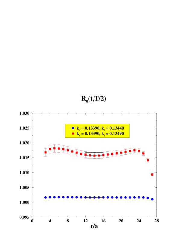
Figure 1: Time dependence of the double ratio (15), averaged between the two halves of the lattice, for two sets of quark masses, given in the legend. The plateaux are taken from $t/a=12$ to $t/a=16$.

There are several crucial advantages in the use of the double ratio (15). First, there is a large reduction of statistical uncertainties, because fluctuations in the numerator and the denominator are highly correlated. Second, the matrix elements of the meson sources, $\sqrt{Z_{K}}$ and $\sqrt{Z_{\pi}}$, appearing in Eq. (10), cancel between numerator and denominator. Third, the double ratio is independent from the improved renormalization constant $Z_{V}[1+b_{V}(am_{s}+am_{\ell})/2]$ as well as from the improvement coefficient $c_{V}$ [see Eq. (13)] . Therefore the knowledge of $Z_{V}$, $b_{V}$ and $c_{V}$ is not necessary to compute $R_{0}$ and this ratio is automatically improved at order $a^{2}$. Finally, the double ratio is equal to unity in the SU(3)-symmetric limit at all orders in the lattice spacing $a$. Thus the deviation of $R_{0}$ from unity depends on the physical SU(3) breaking effects on $f_{0}(q_{\rm max}^{2})$ as well as on discretization errors, which are at least of order $a^{2}(m_{s}-m_{\ell})^{2}$ (see Section 4.3). A similar consideration applies also to the quenching error, because the double ratio $R_{0}(t_{x},t_{y})$ is correctly normalized to unity in the SU(3)-symmetric limit also in the quenched approximation.

Having chosen $t_{y}=T/2$, the three-point correlation functions are symmetric between the two halves $0<t_{x}<T/2$ and $T/2<t_{x}<T$. Statistical fluctuations, however, are independent in the two halves of the lattice. The best precision is reached when the double ratio is constructed in the two halves separately and then averaged. We obtain values of $f_{0}(q^{2}_{\rm max})$ with an uncertainty smaller than $0.1\%$, as it can be seen from Table 2 and Fig. 2 (left).

$k_{s}-k_{\ell}$	$~{}~{}~{}~{}a^{2}\Delta M^{2}$	$~{}~{}a^{2}q_{\rm max}^{2}$	$~{}~{}f_{0}(q_{\rm max}^{2})$
$0.13390-0.13440$	$+0.01727(12)$	$0.000737(10)$	$0.99991(6)$
$0.13390-0.13490$	$+0.03316(26)$	$0.00365(6)$	$1.0018(5)$
$0.13390-0.13520$	$+0.04225(34)$	$0.00745(15)$	$1.010(2)$
$0.13440-0.13390$	$-0.01777(12)$	$0.000665(8)$	$0.99974(6)$
$0.13440-0.13490$	$+0.01634(15)$	$0.000988(21)$	$1.0008(2)$
$0.13440-0.13520$	$+0.02565(23)$	$0.00312(8)$	$1.0057(9)$
$0.13490-0.13390$	$-0.03496(30)$	$0.00279(5)$	$0.9993(4)$
$0.13490-0.13440$	$-0.01674(17)$	$0.000832(18)$	$1.0002(2)$
$0.13490-0.13520$	$+0.00948(10)$	$0.000497(15)$	$1.0014(2)$
$0.13520-0.13390$	$-0.04491(46)$	$0.00484(11)$	$1.000(1)$
$0.13520-0.13440$	$-0.02646(31)$	$0.00222(6)$	$1.0015(7)$
$0.13520-0.13490$	$-0.00955(12)$	$0.000416(13)$	$1.0009(2)$
$0.13385-0.13433$	$+0.01682(7)$	$0.000669(6)$	$0.99995(5)$
$0.13385-0.13501$	$+0.03821(24)$	$0.00519(6)$	$1.0047(7)$
$0.13433-0.13385$	$-0.01731(7)$	$0.000610(6)$	$0.99977(5)$
$0.13433-0.13501$	$+0.02205(15)$	$0.00193(3)$	$1.0022(5)$
$0.13501-0.13385$	$-0.04093(22)$	$0.00380(5)$	$0.9995(6)$
$0.13501-0.13433$	$-0.02295(15)$	$0.00154(2)$	$1.0008(3)$

Table 2: Values of the hopping parameters $k_{s}$ and $k_{\ell}$, $a^{2}\Delta M^{2}$, $a^{2}q_{\rm max}^{2}$ and $f_{0}(q_{\rm max}^{2})$ obtained with the double ratio method [see Eq. (16)].

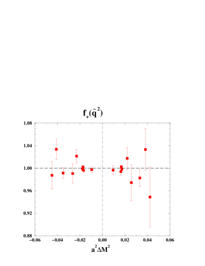
Figure 2: Values of $f_{0}(q_{\rm max}^{2})$ (left) and $f_{+}(\bar{q}^{2})$ (right) as a function of the SU(3)-breaking parameter $a^{2}\Delta M^{2}=a^{2}M_{K}^{2}-a^{2}M_{\pi}^{2}$. The dependence on $q_{\rm max}^{2}$ and $\bar{q}^{2}$ is not explicitly shown in the plots.

By replacing in Eq. (15) the time component of the vector current with the spatial ones and setting $a\vec{p}=a\vec{p}^{\,\prime}=\pi/12~{}(1,0,0)$ (the minimum non-zero momentum allowed on our lattice), also the form factor $f_{+}$ can be extracted from the double ratio

$${\displaystyle{C_{1}^{K\pi}(t_{x},t_{y},\vec{p},\vec{p})\,C_{1}^{\pi K}(t_{x},t_{y},\vec{p},\vec{p})\over C_{1}^{KK}(t_{x},t_{y},\vec{p},\vec{p})\,C_{1}^{\pi\pi}(t_{x},t_{y},\vec{p},\vec{p})}}\left.{}_{\overrightarrow{\stackrel{{\scriptstyle\mbox{\tiny$t_{x}\to\infty$}}}{{\mbox{\tiny$(t_{y}-t_{x})\to\infty$}}}}}\right.[f_{+}(\bar{q}^{2})]^{2}\,.$$ (17)

where $\bar{q}^{2}=\left(\sqrt{M_{K}^{2}+|\vec{p}|^{2}}-\sqrt{M_{\pi}^{2}+|\vec{p}|^{2}}\right)^{2}<q_{\rm max}^{2}$. The uncertainty obtained in this case, however, is about twenty times larger than the one obtained for $f_{0}(q^{2}_{\rm max})$, as shown in Fig. 2.

4 Momentum dependence of the form factors and extrapolation to $q^{2}=0$

In this Section we perform the extrapolation of the scalar form factor from $q_{\rm max}^{2}$ to $q^{2}=0$. To this end we need to evaluate the slope of $f_{0}$, which in turn means to study the $q^{2}$-dependence of the scalar form factor. We stress that, in order to obtain $f_{0}(0)$ at the percent level, the precision required for the slope can be much lower, since the values of $q_{\rm max}^{2}$ used in our lattice calculations are quite close to $q^{2}=0$ (see Table 2). We find indeed that a $\simeq 30\%$ precision is enough for our purposes.

The form factors $f_{0}(q^{2})$ and $f_{+}(q^{2})$ can be expressed as linear combinations of the matrix elements $\langle\pi|\hat{V}_{\mu}|K\rangle$. Their $q^{2}$-dependence is obtained by studying these matrix elements determined according to Eq. (12) for the set of momenta listed in Table 1, using both time and spatial components of the vector current.

The renormalization constant $Z_{V}$ of the lattice vector current and the improvement coefficients $b_{V}$ and $c_{V}$ are needed in the calculation. In order to minimize the statistical fluctuations we have calculated $Z_{V}$ and $b_{V}$ on the same sets of gauge configurations and combinations of quark masses used in the study of the form factors.

4.1 Evaluation of $Z_{V}$ and $b_{V}$

The vector current renormalization constant, $Z_{V}$, and the improvement coefficient, $b_{V}$, can be extracted from the following relation

$${\displaystyle{1\over 2}}{\displaystyle{C^{K(\pi)}(T/2,\vec{0})\over C_{0}^{KK(\pi\pi)}(t_{x},T/2,\vec{0},\vec{0})}}=Z_{V}(1+b_{V}am_{q})+\mathcal{O}(a^{2})\,,$$ (18)

where $am_{q}=(1/k_{s}-1/k_{c})/2$ for $K\to K$ transitions and $am_{q}=(1/k_{\ell}-1/k_{c})/2$ for $\pi\to\pi$ ones. The results obtained for the l.h.s. of Eq. (18) show a clear linear dependence on the quark mass $am_{q}$. A linear fit yields

$$Z_{V}=0.7876\pm 0.0002\,, b_{V}=1.393\pm 0.006\,,$$ (19)

in excellent agreement with the findings of Refs. [14]-[16]. In what follows we use the values of $Z_{V}$ and $b_{V}$ given in Eq. (19) and adopt for the improvement coefficient $c_{V}$ the non-perturbative value $c_{V}=-0.09$ from Ref. [14].

4.2 $q^{2}$-dependence of $f_{0}$ and $f_{+}$

The form factors $f_{0}(q^{2})$ and $f_{+}(q^{2})$ are shown in Fig. 3 as a function of $q^{2}$. Note that, although we considered only ten independent combinations of meson momenta (see Table 1), we have computed both $K\to\pi$ and $\pi\to K$ amplitudes, obtaining in this way twenty different values of $q^{2}$. The form factor $f_{+}(q^{2})$ is rather well determined with a statistical error of $\simeq 5\div 20\%$, whereas for the scalar form factor the uncertainties turn out to be about $5$ times larger.

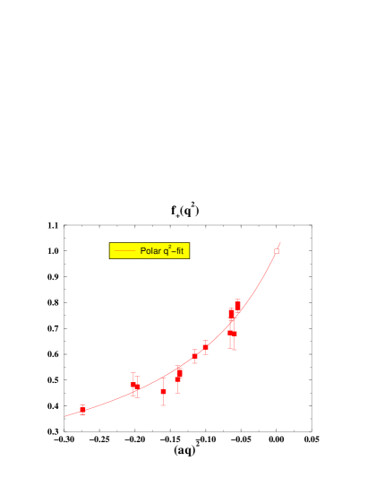
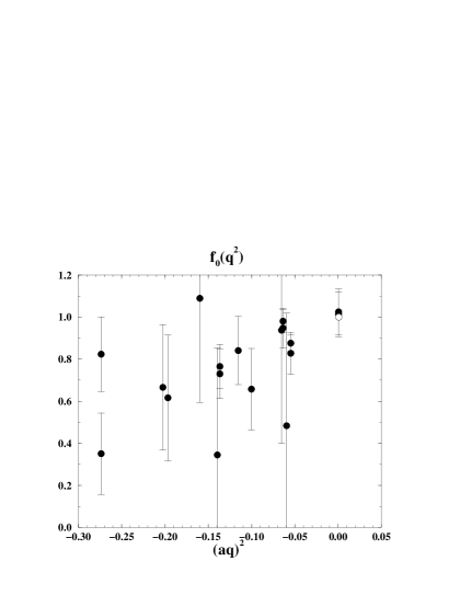
Figure 3: Values of the form factors $f_{+}(q^{2})$ (left) and $f_{0}(q^{2})$ (right) as a function of the four-momentum square $(aq)^{2}$, for the quark mass combination $k_{s}=0.13390$ and $k_{\ell}=0.13440$. Open markers represent the results obtained with the double ratio method; the errors on these points are smaller than the size of the markers. In the left picture the solid line is the pole-dominance fit (20).

Our results for $f_{+}(q^{2})$ are very well described by a pole-dominance fit, viz.

$$f_{+}(q^{2}) = {\displaystyle{f_{+}(0)\over 1-\lambda_{+}\,q^{2}}}\,,$$ (20)

as illustrated by the solid line in Fig. 3. The values obtained for the slope $\lambda_{+}$ agree well with the inverse of the $K^{*}$-meson mass square for each combination of the simulated quark masses. A simple linear extrapolation in terms of the quark masses to the physical values yields $\lambda_{+}=0.026\pm 0.002$ in units of the physical value of $M_{\pi^{+}}^{2}$, which is consistent with the PDG value $\lambda_{+}=0.028\pm 0.002$ [17] as well as with the recent measurement from KTeV $\lambda_{+}=0.02502\pm 0.00037$ [18], obtained using a pole parameterization. The polar fit (20) also provides the value of $f_{+}(0)$. Due to the uncertainties in the determination of $f_{+}(q^{2})$, however, the values obtained for $f_{+}(0)$ have statistical errors well above $1\%$, which do not allow to investigate SU(3)-breaking effects. The only way to keep these errors below $1\%$ is to use the high-precision results obtained for $f_{0}(q_{\rm max}^{2})$. This in turn requires a drastic improvement in the evaluation of the scalar form factor as a function of $q^{2}$. To this end, we have considered an alternative procedure based on the introduction of suitable double ratios, namely

$$R_{i}(t_{x},t_{y})={\displaystyle{C_{i}^{K\pi}(t_{x},t_{y},\vec{p},\vec{p}^{\,\prime})\over C_{0}^{K\pi}(t_{x},t_{y},\vec{p},\vec{p}^{\,\prime})}}~{}{\displaystyle{C_{0}^{KK}(t_{x},t_{y},\vec{p},\vec{p}^{\,\prime})\over C_{i}^{KK}(t_{x},t_{y},\vec{p},\vec{p}^{\,\prime})}}~{},$$ (21)

from which a determination of the ratio of the form factors $f_{0}(q^{2})/f_{+}(q^{2})$ can be obtained. The advantages of the double ratios (21) are similar to those already pointed out for the double ratio (15), namely: i) a large reduction of statistical fluctuations; ii) the independence of the renormalization constant $Z_{V}$ and the improvement coefficient $b_{V}$, and iii) $R_{i}\to 1$ in the SU(3)-symmetric limit. We stress that the introduction of the matrix elements of degenerate mesons in Eq. (21) is crucial to largely reduce statistical fluctuations, because it compensates the different fluctuations of the matrix elements of the spatial and time components of the weak current.

By denoting with $\overline{R}_{i}(q^{2})$ the plateaux of the double ratios $R_{i}(t_{x},t_{y})$ at enough large time distances, the ratio $f_{0}(q^{2})/f_{+}(q^{2})$ is given by

$${\displaystyle{f_{0}(q^{2})\over f_{+}(q^{2})}}=1+{\displaystyle{q^{2}\over M_{K}^{2}-M_{\pi}^{2}}}\,{\displaystyle{-(E_{K}+E_{K}^{\prime})\,(p+p^{\prime})_{i}+(E_{K}+E_{\pi})(p+p^{\prime})_{i}\,\overline{R}_{i}(q^{2})\over(E_{K}+E_{K}^{\prime})\,(p-p^{\prime})_{i}-(E_{K}-E_{\pi})(p+p^{\prime})_{i}\,\overline{R}_{i}(q^{2})}}\,,$$ (22)

where $E_{K}^{\prime}\equiv\sqrt{M_{K}^{2}+|\vec{p}^{\,\prime}|^{2}}$. The $q^{2}$-behavior of $f_{0}(q^{2})$ can be then investigated after multiplying the ratio $f_{0}(q^{2})/f_{+}(q^{2})$, obtained from Eq. (22), by the values of $f_{+}(q^{2})$ obtained with the standard procedure. The statistical uncertainties on $\overline{R}_{i}(q^{2})$ and $f_{0}(q^{2})$ turn out to be $\simeq 1\div 20\%$ and $\simeq 5\div 20\%$, respectively. The quality of the results for $f_{0}(q^{2})$, obtained in this way, is illustrated in Fig. 4 for one of the eighteen combinations of quark masses. These results can be directly compared with those obtained by using the standard method and shown in Fig. 3 (right).

In order to extrapolate the scalar form factor to zero-momentum transfer we have considered three different possibilities, namely a polar, a linear and a quadratic fit:

$$f_{0}(q^{2}) = f_{0}^{(pol.)}(0)/(1-\lambda_{0}^{(pol.)}\,q^{2})\,,$$ (23)

$$f_{0}(q^{2}) = f_{0}^{(lin.)}(0)\cdot(1+\lambda_{0}^{(lin.)}\,q^{2})\,,$$ (24)

$$f_{0}(q^{2}) = f_{0}^{(quad.)}(0)\cdot(1+\lambda_{0}^{(quad.)}\,q^{2}+c_{0}\,q^{4})\,.$$ (25)

These fits are shown in Fig. 4.

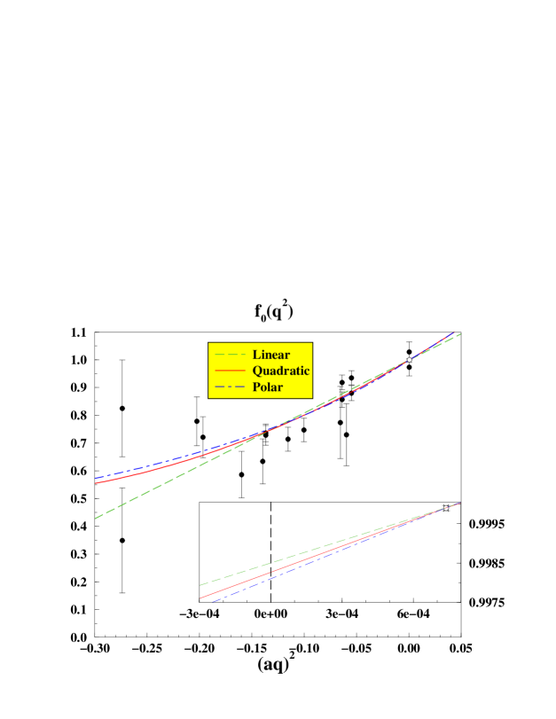
Figure 4: The form factor $f_{0}(q^{2})$ obtained from the double ratios (21) for $q^{2}<q_{\rm max}^{2}$ (full dots) and from the double ratio (15) at $q^{2}=q_{\rm max}^{2}$ (open dot), for the quark mass combination $k_{s}=0.13390$ and $k_{\ell}=0.13440$. The dot-dashed, dashed and solid lines correspond to the polar, linear and quadratic fits given in Eqs. (23-25), respectively. The inset is an enlargement of the region around $q^{2}=0$.

The polar, linear and quadratic forms fit our results for all quark masses with comparable $\chi^{2}$ values. The three fits provide both $f_{0}(0)$ and the slope $\lambda_{0}$ with values consistent with each other within the statistical uncertainties. Although tiny, the differences found for $f_{0}(0)$ are appreciable with respect to the size of the physical SU(3)-breaking effects. Consequently, for each combination of quark masses we consider all three extrapolated values of $f_{0}(0)$ and treat the difference as a systematic uncertainty in the rest of our analysis. The results obtained for $f_{0}(0)$ and the slope $\lambda_{0}$ are collected in Table 3.

$k_{s}-k_{\ell}$	$f_{0}^{(pol.)}(0)$	$\lambda_{0}^{(pol.)}$	$f_{0}^{(lin.)}(0)$	$\lambda_{0}^{(lin.)}$	$f_{0}^{(quad.)}(0)$	$\lambda_{0}^{(quad.)}$
$0.13390-0.13440$	$0.9981(3)$	$2.5(3)$	$0.9985(2)$	$1.9(2)$	$0.9983(3)$	$2.2(4)$
$0.13390-0.13490$	$0.9912(16)$	$2.9(4)$	$0.9941(10)$	$2.1(2)$	$0.9915(15)$	$2.8(4)$
$0.13390-0.13520$	$0.9858(41)$	$3.2(6)$	$0.9928(22)$	$2.2(3)$	$0.9858(40)$	$3.2(6)$
$0.13440-0.13390$	$0.9981(2)$	$2.4(3)$	$0.9985(1)$	$1.9(2)$	$0.9984(2)$	$2.1(3)$
$0.13440-0.13490$	$0.9975(5)$	$3.3(5)$	$0.9983(3)$	$2.5(3)$	$0.9976(5)$	$3.2(5)$
$0.13440-0.13520$	$0.9940(21)$	$3.7(7)$	$0.9972(13)$	$2.7(4)$	$0.9946(19)$	$3.5(7)$
$0.13490-0.13390$	$0.9923(11)$	$2.5(3)$	$0.9941(7)$	$1.9(2)$	$0.9931(11)$	$2.3(3)$
$0.13490-0.13440$	$0.9978(4)$	$2.9(4)$	$0.9984(3)$	$2.2(2)$	$0.9980(4)$	$2.7(4)$
$0.13490-0.13520$	$0.9993(4)$	$4.3(9)$	$0.9998(3)$	$3.3(5)$	$0.9996(4)$	$3.6(9)$
$0.13520-0.13390$	$0.9882(22)$	$2.5(3)$	$0.9912(16)$	$1.8(2)$	$0.9894(21)$	$2.2(3)$
$0.13520-0.13440$	$0.9951(13)$	$2.9(4)$	$0.9967(10)$	$2.2(3)$	$0.9955(11)$	$2.7(4)$
$0.13520-0.13490$	$0.9993(3)$	$3.9(7)$	$0.9997(3)$	$2.9(4)$	$0.9995(3)$	$3.4(7)$
$0.13385-0.13433$	$0.9982(3)$	$2.6(4)$	$0.9986(2)$	$2.0(2)$	$0.9986(3)$	$1.9(5)$
$0.13385-0.13501$	$0.9863(34)$	$3.5(7)$	$0.9913(17)$	$2.6(3)$	$0.9923(34)$	$2.4(7)$
$0.13433-0.13385$	$0.9981(2)$	$2.7(4)$	$0.9985(1)$	$2.0(2)$	$0.9985(3)$	$2.1(4)$
$0.13433-0.13501$	$0.9945(15)$	$4.0(8)$	$0.9966(9)$	$2.9(4)$	$0.9971(14)$	$2.7(7)$
$0.13501-0.13385$	$0.9880(16)$	$3.0(4)$	$0.9913(9)$	$2.2(2)$	$0.9902(16)$	$2.5(4)$
$0.13501-0.13433$	$0.9959(8)$	$3.2(5)$	$0.9972(5)$	$2.4(3)$	$0.9969(8)$	$2.5(5)$

Table 3: The form factor at zero-momentum $f_{0}(0)$ and its slope $\lambda_{0}$, obtained from the three fits (23-25), for all combinations of the hopping parameters.

Before closing this Section we mention that our results for the slope $\lambda_{0}$, extrapolated to the physical meson masses using a linear dependence in the quark masses, give in units of the physical value of $M_{\pi^{+}}^{2}$: $\lambda_{0}^{(pol.)}=0.0122(22)$, $\lambda_{0}^{(lin.)}=0.0089(11)$ and $\lambda_{0}^{(quad.)}=0.0115(26)$. Our “polar” value $\lambda_{0}^{(pol.)}$ is consistent with the recent determination from KTeV $\lambda_{0}=0.01414\pm 0.00095$ [18], obtained using a pole parameterization.

4.3 Discretization effects

Lattice artifacts on $f_{0}(0)$ due to the finiteness of the lattice spacing start at ${\cal O}(a^{2})$ and are proportional to $(m_{s}-m_{\ell})^{2}$, like the physical SU(3)-breaking effects. Indeed, the determination of $f_{0}(q_{\rm max}^{2})$ is affected only by discretization errors of ${\cal O}[a^{2}(m_{s}-m_{\ell})^{2}]$, because the double ratio (15) is ${\cal O}(a)$-improved and symmetric with respect to the exchange $m_{s}\leftrightarrow m_{\ell}$ in the weak vertex. In addition, since $q_{\rm max}^{2}$ is proportional to $(m_{s}-m_{\ell})^{2}$, ${\cal O}(a^{2})$ effects in the extrapolation from $q_{\rm max}^{2}$ to $q^{2}=0$ also vanish quadratically in $(m_{s}-m_{\ell})$. Being in our calculation $a^{-1}\simeq 2.7$ GeV, we expect discretization errors to be sensibly smaller than the physical SU(3)-breaking effects.

A qualitative estimate of discretization errors can be obtained by considering the effect of the terms proportional to the improvement coefficient $b_{V}$, which cancel out at first order in the double ratio (15), but contribute at second order. A simple calculation shows that this correction is given by $[1+b_{V}(am_{s}+am_{\ell})/2]^{2}/[(1+b_{v}am_{s})\cdot(1+b_{V}am_{\ell})]\simeq 1-a^{2}b_{V}^{2}(m_{s}-m_{\ell})^{2}/4$. The size of such a ${\cal O}(a^{2})$ contribution is a few percent of the whole result. Calculations performed at different values of the lattice spacing, combined with the extrapolation to the continuum limit, will certainly allow a quantitative estimate of discretization errors and a further reduction of this source of uncertainty.

In Fig. 5 we plot the values of $f_{0}(0)$, obtained from the fit in $q^{2}$ given by Eq. (25), versus $(a^{2}\Delta M^{2})^{2}$. The results agree well with the quadratic dependence on $a^{2}\Delta M^{2}$, expected from both physical and lattice artifact contributions, as shown in Fig. 5 by the solid line representing a naïve fit to the form

$$f_{0}(0)=1-A~{}(a^{2}\Delta M^{2})^{2}~{},$$ (26)

where $A$ is a mass-independent parameter.

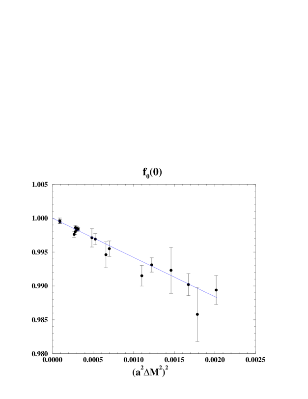
Figure 5: Values of $f_{0}(0)$, obtained from the quadratic fit (25), versus $(a^{2}\Delta M^{2})^{2}$. The solid line is the result of the linear fit (26).

5 Extraction of $\Delta f$

In order to determine the physical value of $f_{0}(0)$, we need to extrapolate our results of Table 3 to the physical kaon and pion masses. As discussed in the introduction, the problem of the chiral extrapolation is substantially simplified if we remove the effect of the leading chiral logs. To this purpose we consider the quantity

$$\Delta f=1+f_{2}-f_{0}(0)\,,$$ (27)

where $f_{2}$ represents the leading non-local contribution determined by pseudoscalar meson loops within CHPT. This procedure is well defined thanks to the finiteness of the leading non-local contributions both in the quenched and in the unquenched version of the effective theory. Having subtracted the leading logarithmic corrections, we expect $\Delta f$ to receive large contributions from local operators in the effective theory and, as in the case of the $q^{2}$ slopes discussed in Section 4, to be better suited for a smooth polynomial extrapolation in the meson masses.

As pointed out in the Introduction, the subtraction of $f_{2}$ in Eq. (27) does not imply necessarily a good convergence of CHPT at order ${\cal O}(p^{4})$ for the meson masses used in our lattice simulations. The aim of this subtraction is to define a quantity whose chiral expansion starts at order ${\cal O}(p^{6})$ independently of the values of the meson masses, or a quantity better suited for a smooth chiral extrapolation. It is also worth to emphasise that the numerical impact of $f_{2}^{q}$ turns out to be very small (around or below 10 % with respect to the whole value of $\Delta f$) for the highest meson masses used in our simulations. It increases (without exceeding 30 % of $\Delta f$) in the case of lighter masses, where the chiral expansion should have a better convergence.

5.1 Chiral loops within full QCD

In the isospin-symmetric limit, within full QCD, the expression of the leading chiral correction $f_{2}$ is [3]

$$f_{2}={3\over 2}H_{\pi K}+{3\over 2}H_{\eta K}\;,$$ (28)

where

$$H_{PQ}=-{1\over 64\pi^{2}f_{\pi}^{2}}\left[M_{P}^{2}+M_{Q}^{2}+{2M_{P}^{2}M_{Q}^{2}\over M_{P}^{2}-M_{Q}^{2}}\log{\left(M_{Q}^{2}\over M_{P}^{2}\right)}\right]\;\;.$$ (29)

Note that $f_{2}$ is completely specified in terms of pseudoscalar meson masses and decay constants ($f_{\pi}\approx 132$ MeV); it is negative ($f_{2}\approx-0.023$ for physical masses), as implied by unitarity [3, 19]; it vanishes as $(M_{K}^{2}-M_{\pi}^{2})^{2}/(f_{\pi}^{2}M_{K}^{2})$ in the SU(3) limit, following the combined constraints of chiral symmetry and the Ademollo-Gatto theorem.

5.2 Chiral loops within quenched QCD

The structure of chiral logarithms appearing in Eqs. (28)–(29), is valid only in the full theory. In the quenched theory, the leading (unphysical) logarithms are instead those entering the one-loop functional of qCHPT [9, 10, 11]. We calculated this correction and present the results in this Section. Normalizing the lowest-order qCHPT Lagrangian as in Ref. [9], with a quadratic term for the singlet field $\Phi_{0}={\rm str}(\Phi)$ chosen as

$$\left.{\cal L}^{q}_{2}\right|_{\Phi^{2}_{0}}=\frac{\alpha}{6}D_{\mu}\Phi_{0}D^{\mu}\Phi_{0}-\frac{M_{0}^{2}}{6}\Phi_{0}^{2}~{},$$ (30)

we find

$$f_{2}^{q}=H^{q}_{\pi K}+H^{q}_{(s\bar{s})K}~{},$$ (31)

where

$$H^{q}_{PK}=\frac{M_{K}^{2}}{96\pi^{2}f_{\pi}^{2}}\left[\frac{M_{0}^{2}(M_{K}^{2}+M_{P}^{2})-2\alpha M_{K}^{2}M_{P}^{2}}{{\left(M_{K}^{2}-M_{P}^{2}\right)}^{2}}\,\log\left(\frac{M_{K}^{2}}{M_{P}^{2}}\right)-\,\alpha\right]$$ (32)

with $M_{(s\bar{s})}^{2}=2M_{K}^{2}-M_{\pi}^{2}$. As anticipated, the one-loop result in Eq. (31) is finite because of the Ademollo-Gatto theorem, which is still valid in the quenched approximation [9] and forbids the appearance of contributions from local operators in $f^{q}_{2}$. A proof beyond the one-loop level that the Ademollo-Gatto theorem (and more generally the Sirlin’s relation [20]) holds within qCHPT can easily be obtained by applying the functional formalism to the demonstration in Ref. [20]. The latter needs only flavor symmetries which hold on the lattice also in the quenched case.

It is worth to emphasize that the nature of the SU(3) breaking corrections in the quenched theory is completely different from that of full QCD: only contributions coming from the mixing with the flavor-singlet state are present and one finds $f^{q}_{2}>0$, which is a signal of the non-unitarity of the theory. For typical values of the singlet parameters ($M_{0}\approx 0.6$ GeV and $\alpha\approx 0$ [21]) and for the physical values of pion and kaon masses, one finds $f^{q}_{2}\approx+0.022$. For the quark masses used in the simulation (and at the same values of $M_{0}$ and $\alpha$), the non-local correction is substantially smaller, $f^{q}_{2}<0.003$. This estimate is not changed significantly if a value of $M_{0}$ as large as $1$ GeV and/or a $20\%$ variation of $f_{\pi}$ are considered. We anticipate that the effect of the above-mentioned variations of $M_{0}$ and/or $f_{\pi}$ on our final result for $\Delta f$ is within $20\%$ and it has been included in the quoted final uncertainties [see later Eq. (37)]. The reason why in Fig. 5 all values of $f_{0}(0)$ are found to be smaller than unity, as expected in a unitary theory, may be that for these sets of masses the contribution of local operators dominates over the quenched chiral logs.

The high level of accuracy required in the study of the $K_{\ell 3}$ form factors can only be achieved once all possible sources of systematic errors are shown to be kept well under control. In a lattice calculation this includes in particular a study of finite volume effects. In our case such effects are expected to be smaller than other systematic effects, as we have explicitly checked by performing the analytical calculation presented in the Appendix and based on the techniques discussed in Refs. [22, 23].

5.3 Extrapolation to the physical masses

The evaluation of $f_{2}^{q}$ allows to express the lattice results in terms of the subtracted quantity $\Delta f$ defined in Eq. (27). To study the dependence of this quantity on the meson masses it is convenient to divide $\Delta f$ by $(\Delta M^{2})^{2}$:

$$R(M_{K},M_{\pi})={\displaystyle{\Delta f\over(a^{2}\Delta M^{2})^{2}}}={\displaystyle{1+f^{q}_{2}(M_{K},M_{\pi})-f_{0}(0;M_{K},M_{\pi})\over(a^{2}\Delta M^{2})^{2}}}~{}.$$ (33)

We have used $f_{2}^{q}$ computed from Eq. (31) at the corresponding values of meson masses, setting $M_{0}=0.6\,$GeV and $\alpha=0.05$. The error induced by a variation of $M_{0}$ and $\alpha$ in a reasonable range of values is found to be negligible compared to the statistical error. We find that at the simulated masses the effect of $f_{2}^{q}$ does not exceed $30\%$ of the value of $[1-f_{0}(0)]$. Since $f_{2}^{q}$ has a non-trivial, non-analytic dependence from the quark masses, we subtract its contribution at each value of the quark masses.

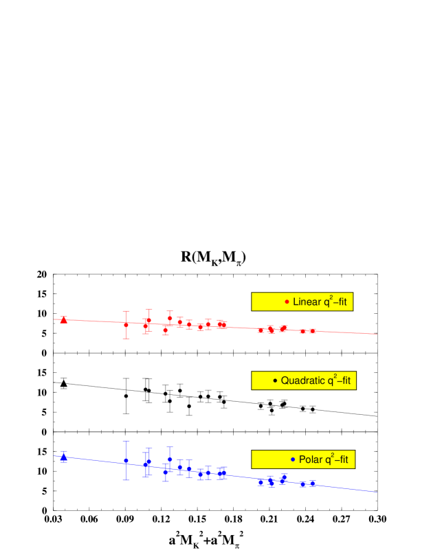
Figure 6: $R(M_{K},M_{\pi})$ as a function of $[a^{2}M_{K}^{2}+a^{2}M_{\pi}^{2}]$ for the cases of the linear, quadratic and polar $q^{2}$-extrapolation in the fit of $f_{0}(q^{2})$. The solid lines represent the results of the linear fit (34). Triangles indicate the values of $R(M_{K},M_{\pi})$ extrapolated to the physical kaon and pion masses.

As shown in Fig. 6, the dependence of $R(M_{K},M_{\pi})$ on the squared meson masses is well described by a simple linear fit:

$$R(M_{K},M_{\pi})=c_{11}+c_{12}[(aM_{K})^{2}+(aM_{\pi})^{2}]~{},$$ (34)

whereas the dependence on $\Delta M^{2}$ is found to be negligible. We find an excellent $\chi^{2}$ for all the three sets of values of $f_{0}(0)$ obtained from the linear, quadratic and polar extrapolation in $q^{2}$, see Fig. 6. In order to check the stability of the results, we have also performed quadratic and logarithmic fits, viz.

$$R(M_{K},M_{\pi}) = c_{21}+c_{22}[(aM_{K})^{2}+(aM_{\pi})^{2}]+c_{23}[(aM_{K})^{2}+(aM_{\pi})^{2}]^{2}\,,$$ (35)

$$R(M_{K},M_{\pi}) = c_{31}+c_{32}\log[(aM_{K})^{2}+(aM_{\pi})^{2}]\,.$$ (36)

It is reassuring to find that, while increasing the number of parameters in the chiral extrapolation as done in the quadratic fit (35) leads to larger uncertainties, the shift in the central values remains smaller than the errors. The logarithmic fit has been considered in order to investigate the presence of possible important non-analytical terms in $R(M_{K},M_{\pi})$. In Fig. 7 we show that linear, quadratic and logarithmic functional forms provide equally good fits of the data with consistent results for the extrapolation to the physical point.

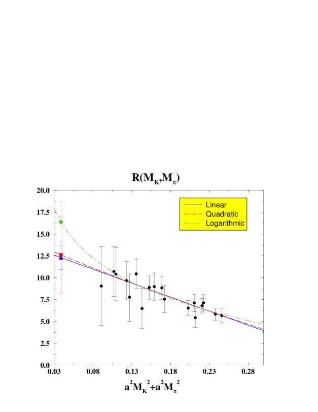
Figure 7: Comparison among linear (34), quadratic (35) and logarithmic (36) fits of the ratio $R(M_{K},M_{\pi})$ as a function of $[a^{2}M_{K}^{2}+a^{2}M_{\pi}^{2}]$. Triangle, square and diamond represent the values of $R(M_{K},M_{\pi})$ extrapolated to the physical meson masses. For illustrative purposes we have chosen the case in which a quadratic $q^{2}$-dependence of $f_{0}(q^{2})$ has been used to extrapolate the scalar form factor to $q^{2}=0$.

	Linear Fit	Quadratic Fit	Logarithmic Fit
Linear $f_{0}(q^{2})$	$0.009\pm 0.001$	$0.008\pm 0.003$	$0.011\pm 0.002$
Quadratic $f_{0}(q^{2})$	$0.013\pm 0.002$	$0.014\pm 0.005$	$0.018\pm 0.003$
Polar $f_{0}(q^{2})$	$0.015\pm 0.002$	$0.018\pm 0.005$	$0.020\pm 0.003$

	Linear Fit	Quadratic Fit	Logarithmic Fit
Linear $f_{0}(q^{2})$	$0.012\pm 0.001$	$0.013\pm 0.003$	$0.015\pm 0.002$
Quadratic $f_{0}(q^{2})$	$0.017\pm 0.002$	$0.021\pm 0.004$	$0.023\pm 0.002$
Polar $f_{0}(q^{2})$	$0.019\pm 0.002$	$0.025\pm 0.005$	$0.026\pm 0.003$

Table 4: Results for $\Delta f$ obtained from linear, quadratic and logarithmic fits of the ratio $R(M_{K},M_{\pi})$ assuming linear, quadratic or polar functional forms for the extrapolation of the scalar form factor to $q^{2}=0$. Upper and lower tables correspond to different choices of the time interval chosen for the fits of the two-point correlation functions (see text).

The extrapolated values of $R(M_{K},M_{\pi})$ are converted into predictions for $\Delta f$ by using the values of the physical kaon and pion masses in lattice units given in Section 2. By this procedure, i.e. expressing both $R(M_{K},M_{\pi})$ and the meson masses in lattice units, we get rid of the error associated with the determination of the lattice spacing in the quenched approximation. In Table 4 we collect the values of $\Delta f$ obtained for all the functional forms assumed both in fitting the $q^{2}$-dependence of $f_{0}(q^{2})$ and in extrapolating the ratio $R(M_{K},M_{\pi})$ to the physical meson masses. We present two sets of results. The first set, given in the upper table, is obtained by determining the matrix elements $\sqrt{Z_{K}}$ and $\sqrt{Z_{\pi}}$ [see Eq. (11)] from a fit of the two-point correlation functions in the same time interval chosen for the three-point correlators, namely $t/a\in$ [11,17]. For the second set, given in the lower table, the same time interval chosen to extract the meson masses, i.e. $t/a\in$ [12,26], has been considered.

From the spread of the values in Table 4 we quote our final estimate

$$\Delta f=R(M_{K}^{\rm phys},M_{\pi}^{\rm phys})\times[(a^{2}\Delta M^{2})^{2}]^{\rm phys}=(0.017\pm 0.005_{\rm stat}\pm 0.007_{\rm syst})~{},$$ (37)

where the systematic error is dominated by the extrapolation of $f_{0}(q^{2})$ in $q^{2}$ and of $R(M_{K},M_{\pi})$ in the meson masses.

The result in Eq. (37) is the main result of this paper. We have checked that all other sources of systematic errors, as those originated from different choices of the plateau intervals, from the uncertainties in the values of the renormalization constant $Z_{V}$ and of the improvement coefficients $b_{V}$ and $c_{V}$, and from the estimated size of discretization effects, are negligible with respect to the systematic error quoted in Eq. (37).

6 Estimate of $f_{+}(0)$ and impact on $|V_{us}|$

The value of $\Delta f$ given in Eq. (37) is in excellent agreement with the estimate of $\Delta f$ made by Leutwyler and Roos using a general parameterization of the SU(3) breaking structure of the pseudoscalar-meson wave functions [3]. It must be stressed, however, that our result is the first computation of this quantity using a non-perturbative method based on QCD. Combining our estimate of $\Delta f$ with the physical value of $f_{2}$ from Eq. (28), we finally obtain

$$f_{+}^{K^{0}\pi^{-}}(0)=0.960\pm 0.005_{\rm stat}\pm 0.007_{\rm syst}$$ (38)

to be compared with the value $f_{+}^{K^{0}\pi^{-}}(0)=0.961\pm 0.008$ given in Ref. [7] and quoted by the PDG [17].

6.1 Comparison with other approaches

We now compare our results in Eqs. (37-38) with the recent evaluations of the ${\cal O}(p^{6})$ contributions to $f_{+}(0)$ made in Refs. [4, 6, 25]. In the chiral expansion the whole ${\cal O}(p^{6})$ term can be separated into two terms, coming respectively from meson loops and local terms. Whereas the whole ${\cal O}(p^{6})$ term is scale- and scheme-independent, the two terms separately depend on the renormalization scale and scheme. Leutwyler-Roos assumed that their quark-model estimate represents the whole physical ${\cal O}(p^{6})$ term. In Refs. [4, 6, 25] this result was interpreted instead to represent the contribution due to the local terms only, at the renormalization scale of the $\rho$-meson mass. The full ${\cal O}(p^{6})$ contribution was then obtained by adding the renormalized loop amplitude computed in Ref. [4]. In this way the whole ${\cal O}(p^{6})$ correction is found to be very small, though within a large error. The compensation between local and non-local terms at ${\cal O}(p^{6})$ strongly depends on the choice of the renormalization scale. Indeed, varying the renormalization scale from $\mu_{\overline{\rm MS}}\approx 1$ GeV to $\mu_{\overline{\rm MS}}\approx 0.5$ GeV, the loop contribution to $f_{+}(0)$ changes from $+0.4\%$ to $+3.5\%$ [6].

As pointed out in Ref. [25], the use of dispersion relations could help to solve the scale ambiguity. By means of dispersion relations one obtains complementary constraints on the slope and curvature of $f_{0}(q^{2})$ that, in turn, can be used in conjunction with the chiral calculation of Ref. [4] to determine $f_{+}(0)$. Present data, however, are not accurate enough: the estimate of ${\cal O}(p^{6})$ local terms given in Ref. [25] can only be interpreted as a consistency check of the Leutwyler-Roos ansatz, rather than as a truly independent determination. Finally, it must be stressed that all the purely analytic approaches to the estimate of $f_{+}(0)$ suffer from an intrinsic uncertainty due to the value of $f_{K}/f_{\pi}$ [26].

Both these ambiguities (the scale uncertainties and the dependence on $f_{K}/f_{\pi}$) are not present in our approach. By construction, $\Delta f$ is a scale-independent quantity which includes all contributions beyond ${\cal O}(p^{4})$. We determine this quantity only in terms of meson masses. The main sources of uncertainty in our approach come from the $q^{2}$-dependence of the form factor, the chiral extrapolation and the quenched approximation, but we argue that such uncertainties are included in the systematic error quoted in Eq. (37).

6.2 Impact on $|V_{us}|$

Given the good agreement between our estimate of $f_{+}^{K^{0}\pi^{-}}(0)$ and the value of Refs. [7, 17], our result implies a negligible shift in the determination of $|V_{us}|$ from $K_{\ell 3}$ with respect to those works. Assuming the same experimental inputs, the value computed with our form factor, applying the updated radiative and isospin-breaking corrections of Refs. [6, 24], is $|V_{us}|=0.2202\pm 0.0025$ to be compared with $|V_{us}|=0.2196\pm 0.0026$ of Refs. [7, 17]. As pointed out by several authors, this estimate shows a $\approx 2\sigma$ deviation from the CKM unitarity relation, which yields $|V_{us}|=0.2278\pm 0.0020$, taking into account the recent determination $|V_{ud}|=0.9737\pm 0.0007$ from Ref. [27]. According to our analysis and assuming that the quenching effects do not drastically change our findings, this deviation cannot be attributed to an underestimate of the amount of SU(3) breaking in $f_{+}^{K^{0}\pi^{-}}(0)$.

We stress, however, that the above estimate of $|V_{us}|$ takes into account only the (old) published $K_{\ell 3}$ data. Recently, new results have been presented [28, 29, 30, 31]. For instance, using only the high-statistics $K_{e3}$ results of Refs. [28] and [29], we find substantially higher values, namely $|V_{us}|=0.2275\pm 0.0030$ and $|V_{us}|=0.2255\pm 0.0025$, respectively, which are in good agreement with CKM unitarity. The KTeV findings [29] are also confirmed by the preliminary results presented by KLOE [30] and NA48 [31] at the ICHEP ’04 Conference.

7 Conclusions

We presented a quenched lattice study of the $K\to\pi$ vector form factor at zero-momentum transfer. Our calculation is the first one obtained by using a non-perturbative method based only on QCD, except for the quenched approximation. Our main goal is the determination of the second-order SU(3)-breaking quantity $[1-f_{+}(0)]$, which is necessary to extract $|V_{us}|$ from $K_{\ell 3}$ decays. In order to reach the required level of precision we employed the double ratio method originally proposed in Ref. [8] for the study of heavy-light form factors. We found that this approach allows to calculate the scalar form factor $f_{0}(q^{2})$ at $q^{2}=q_{\rm max}^{2}$ with a statistical uncertainty well below $1\%$.

A second crucial ingredient is the extrapolation of the scalar form factor to $q^{2}=0$. This was performed by fitting accurate results obtained using suitable double ratios of three-point correlation functions. The systematic error due to finite volume effects was evaluated and discretization errors were qualitatively estimated to be a few percent of the deviation of $f_{0}(0)$ from unity. Calculations performed at different values of the lattice spacing, combined with the extrapolation to the continuum limit, will certainly allow a more quantitative estimate of discretization errors and a further reduction of this source of uncertainty. Nevertheless it is reasonable to conclude that the uncertainties coming from the functional dependencies of the scalar form factor on both $q^{2}$ and the meson masses are the dominant contribution to the systematic error.

The leading chiral artifacts of the quenched approximation, $f_{2}^{q}$, were corrected for by means of an analytic calculation in quenched chiral perturbation theory. After this subtraction, the lattice results have been smoothly extrapolated to the physical meson masses. Our final value for $f_{+}^{K^{0}\pi^{-}}(0)$ is

$$f_{+}^{K^{0}\pi^{-}}(0)=0.960\pm 0.005_{\rm stat}\pm 0.007_{\rm syst}=0.960\pm 0.009~{},$$ (39)

where the systematic error does not include an estimate of quenched effects beyond ${\cal O}(p^{4})$.

The impact of our result on the determination of $|V_{us}|$ was also addressed. Using the (old) published $K_{\ell 3}$ data from Ref. [17], we obtain $|V_{us}|=0.2202\pm 0.0025$, which still implies a $\approx 2\sigma$ deviation from the CKM unitarity relation. We stress that, according to our analysis, such a deviation should not be attributed to an underestimate of the amount of SU(3) breaking effects in $f_{+}^{K^{0}\pi^{-}}(0)$. Using only the recent high-statistics $K_{e3}$ results of Refs. [28, 29] one finds substantially higher values, $|V_{us}|=0.2275\pm 0.0030$ and $|V_{us}|=0.2255\pm 0.0025$, which are in good agreement with CKM unitarity.

In order to reach a precision better than $1\%$ in the determination of the Cabibbo angle both theoretical and experimental improvements are needed. As for the experimental side, new high-statistics results on both charged and neutral $K_{\ell 3}$ modes are called for. As for the theoretical side, the next important steps are: i) to remove the quenched approximation; ii) to decrease the values of the simulated meson masses in order to gain a better control over the chiral extrapolation of lattice results, and iii) to use larger lattice volumes for decreasing lattice momenta, in order to improve the determination of the slope of the scalar form factor.

Appendix

In this Appendix we present the results of the analytic calculation of finite volume corrections to $f_{2}$, both in the quenched and unquenched theory.

An important advantage of the effective theory approach is that it allows to evaluate (and eventually to correct for) the lattice artifacts due to a finite volume. This is simply achieved by imposing periodic boundary conditions to the wave functions of the chiral fields. This approximation represents a good description of the finite-volume effects as long as the size $L$ of the lattice satisfies the condition $L\cdot M_{\pi,K}\gg 1$ [22], which is well satisfied in the present simulation.

Defining the finite-volume shifts as

$$\delta_{L}=\left.f_{2}\right|_{L}-f_{2}\,,$$ (40)

we find that the corrections to Eqs. (28) and (31) are given by

$$\delta_{L} = -\frac{3}{8\,f_{\pi}^{2}}\left[2\,\xi_{\frac{1}{2}}(L,M_{K})+\xi_{\frac{1}{2}}(L,M_{\pi})+\xi_{\frac{1}{2}}(L,M_{\eta})\right.$$ (41)

$$\qquad\left.-2\,\xi_{\frac{1}{2}}(L,M_{\pi},M_{K})-2\,\xi_{\frac{1}{2}}(L,M_{\eta},M_{K})\right]\,,$$

$$\delta_{L}^{q} = \frac{1}{72\,f_{\pi}^{2}}\left[-2\,\frac{\left(5\,M_{K}^{2}\,\alpha-4\,M_{\pi}^{2}\,\alpha-M_{0}^{2}\right)}{M_{K}^{2}-M_{\pi}^{2}}\,\left(\xi_{\frac{1}{2}}(L,M_{\pi})-\xi_{\frac{1}{2}}(L,M_{(s\bar{s})})\right)\right.$$ (42)

$$\qquad\left.+3\,\left(M_{0}^{2}-\alpha\,M_{\pi}^{2}\right)\,\xi_{\frac{3}{2}}(L,M_{\pi})+3\,\left(M_{0}^{2}-\alpha\,M_{(s\bar{s})}^{2}\right)\,\xi_{\frac{3}{2}}(L,M_{(s\bar{s})})\right.$$

$$\qquad\left.-12\,\frac{\left(M_{K}^{2}\,\alpha-M_{0}^{2}\right)}{M_{K}^{2}-M_{\pi}^{2}}\,\left(\xi_{\frac{1}{2}}(L,M_{\pi},M_{K})-\xi_{\frac{1}{2}}(L,M_{(s\bar{s})},M_{K})\right)\right.$$

$$\qquad\left.+8\,\left(M_{(s\bar{s})}^{2}\,\alpha-M_{0}^{2}\right)\,\xi_{\frac{3}{2}}(L,M_{\pi},M_{(s\bar{s})})+12\,\left(M_{\pi}^{2}\,\alpha-M_{0}^{2}\right)\,\xi^{\prime}_{\frac{1}{2}}(L,M_{K},M_{\pi})\right.$$

$$\qquad\left.+12\,\left(M_{(s\bar{s})}^{2}\,\alpha-M_{0}^{2}\right)\,\xi^{\prime}_{\frac{1}{2}}(L,M_{K},M_{(s\bar{s})})\right]\,,$$

in the unquenched and quenched cases, respectively. The functions $\xi_{s}$ are defined as

$$\xi_{s}(L,M_{1})=\xi_{s}(L,M_{1},M_{1}) = \frac{1}{\Gamma(s)}\int_{0}^{\infty}d\tau\,\tau^{s-1}e^{-M_{1}^{2}\tau}\left[\frac{1}{L^{3}}\theta^{3}\left(\frac{4\pi^{2}}{L^{2}}\tau\right)-\frac{1}{(4\pi\tau)^{3/2}}\right]\,,$$

$$\xi_{s}(L,M_{1},M_{2}) = \frac{1}{\Gamma(s)}\int_{0}^{\infty}d\tau\,\tau^{s-1}e^{-\frac{M_{1}^{2}+M_{2}^{2}}{2}\,\tau}\left[\frac{\sinh\left(\frac{M_{1}^{2}-M_{2}^{2}}{2}\,\tau\right)}{\left(\frac{M_{1}^{2}-M_{2}^{2}}{2}\,\tau\right)}\right]\,$$

$$\times\left[\frac{1}{L^{3}}\theta^{3}\left(\frac{4\pi^{2}}{L^{2}}\tau\right)-\frac{1}{(4\pi\tau)^{3/2}}\right]\,,$$

$$\xi^{\prime}_{s}(L,M_{1},M_{2}) = -\frac{\partial}{\partial M_{2}^{2}}\xi_{s}(L,M_{1},M_{2})\,,$$ (43)

where $\theta(x)\equiv\sum_{n=-\infty}^{\infty}e^{-x\,n^{2}}$, and they represent the differences between finite volume sums and infinite volume integrals (see Ref. [23] for more details). While $\delta_{L}$ represents a small correction in the range of masses used in the simulation, the effect of $\delta_{L}^{q}$ is not negligible with respect to the size of the quenched logs in Eq. (31). Nevertheless, given the smallness of the leading chiral corrections at the simulated meson masses, we find that the inclusion of finite volume corrections has a negligible effect on our final estimate of $\Delta f$.

References

-
[1]
N. Cabibbo,
Phys. Rev. Lett. 10 (1963) 531;
M. Kobayashi and T. Maskawa, Prog. Theor. Phys. 49 (1973) 652. - [2] M. Ademollo and R. Gatto, Phys. Rev. Lett. 13 (1964) 264.
- [3] H. Leutwyler and M. Roos, Z. Phys. C 25 (1984) 91.
- [4] J. Bijnens and P. Talavera, Nucl. Phys. B 669 (2003) 341 [hep-ph/0303103].
- [5] P. Post and K. Schilcher, Eur. Phys. J. C 25 (2002) 427 [hep-ph/0112352].
- [6] V. Cirigliano, H. Neufeld and H. Pichl, hep-ph/0401173.
- [7] M. Battaglia et al., hep-ph/0304132.
- [8] S. Hashimoto, A. X. El-Khadra, A. S. Kronfeld, P. B. Mackenzie, S. M. Ryan and J. N. Simone, Phys. Rev. D 61 (2000) 014502 [hep-ph/9906376].
- [9] G. Colangelo and E. Pallante, Nucl. Phys. B 520 (1998) 433 [hep-lat/9708005].
- [10] C. W. Bernard and M. F. L. Golterman, Phys. Rev. D 46 (1992) 853 [hep-lat/9204007].
- [11] S. R. Sharpe, Phys. Rev. D 46 (1992) 3146 [hep-lat/9205020].
- [12] M. Luscher, S. Sint, R. Sommer and P. Weisz, Nucl. Phys. B 478 (1996) 365 [hep-lat/9605038].
- [13] C.R. Allton, V. Gimenez, L. Giusti and F. Rapuano, Nucl. Phys. B 489 (1997) 427 [hep-lat/9611021].
- [14] T. Bhattacharya, R. Gupta, W. J. Lee and S. R. Sharpe, Phys. Rev. D 63 (2001) 074505 [hep-lat/0009038]; Nucl. Phys. Proc. Suppl. 106, 789 (2002) [hep-lat/0111001].
- [15] M. Luscher, S. Sint, R. Sommer and H. Wittig, Nucl. Phys. B 491 (1997) 344 [hep-lat/9611015].
- [16] D. Becirevic, V. Gimenez, V. Lubicz, G. Martinelli, M. Papinutto and J. Reyes, hep-lat/0401033.
- [17] K. Hagiwara et al. [Particle Data Group Collaboration], Phys. Rev. D 66 (2002) 010001.
- [18] T. Alexopoulos et al. [KTeV Collaboration], hep-ex/0406003.
- [19] G. Furlan, F.G. Lannoy, C. Rossetti, and G. Segré, Nuovo Cim. 38 (1965) 1747.
- [20] A. Sirlin, Ann. Phys. 61 (1970) 294-314, Phys. Rev. Lett. 43 (1979) 904.
-
[21]
W. Bardeen, E. Eichten and H. Thacker, Phys. Rev. D 69 (2004) 054502.
W. Bardeen, A. Duncan, E. Eichten, N. Isgur and H. Thacker, Phys. Rev. D 65 (2002) 014509. - [22] J. Gasser and H. Leutwyler, Phys. Lett. B 184 (1987) 83.
- [23] D. Becirevic and G. Villadoro, Phys. Rev. D 69 (2004) 054010 [hep-lat/0311028].
- [24] V. Cirigliano, M. Knecht, H. Neufeld, H. Rupertsberger and P. Talavera, Eur. Phys. J. C 23 (2002) 121 [hep-ph/0110153];
- [25] M. Jamin, J. A. Oller and A. Pich, JHEP 02 (2004) 047 [hep-ph/0401080].
- [26] N. H. Fuchs, M. Knecht and J. Stern, Phys. Rev. D 62 (2000) 033003 [hep-ph/0001188].
-
[27]
H. Abele et al., Eur. Phys. J. C33 (2004) 1
[hep-ph/0312150].
K.R. Schubert, talk presented at Lepton Photon 2003, Fermilab (USA), August 11-16, 2003. - [28] A. Sher et al. [E865 Collaboration], Phys. Rev. Lett. 91 (2003) 261802; eConf C0304052 (2003) WG608 [hep-ex/0307053].
- [29] T. Alexopoulos et al. [KTeV Collaboration], hep-ex/0406001.
-
[30]
P. Franzini [Kloe Collaboration], invited talk at the 24th International
Conference on Physics in Collision (PIC ’04), Boston (USA), June 27-29, 2004;
hep-ex/0408150.
M. Antonelli [Kloe Collaboration], talk given at the 32nd International Conference on High Energy Physics (ICHEP ’04), Beijing (China), August 16-22, 2004; http://www.ihep.ac.cn/data/ichep04/ppt/8_cp/8-0811-antonelli-m.pdf. - [31] L. Litov [NA48 Collaboration], talk given at the 32nd International Conference on High Energy Physics (ICHEP ’04), Beijing (China), August 16-22, 2004; http://www.ihep.ac.cn/data/ichep04/ppt/8_cp/8-0432-litov-l.ppt.