Abstract

We discuss the inclusive dilepton cross section for proton (quark)-nucleus collisions at high energies in the very forward rapidity region. Starting from the calculation in the quasi-classical approximation, we include low-$x$ evolution effects in the nucleus and predict leading twist shadowing together with anomalous scaling behaviour.

1 Introduction

There is increasing evidence that hard probes [1] are an excellent tool for analyzing the matter produced in high-energy heavy ion collisions at RHIC [2], especially when calibrated against similar probes in proton-proton and proton (deuteron)-ion reactions [3]. At central rapidities the fact that high-$p_{\bot}$ hadron production in $AA$ reactions is suppressed as compared to the production in $pp$ collisions times the expected number of hard collisions, $N_{coll}$, gave strong support to the idea that dense, hot matter is produced in $AA$ collisions causing jets to loose a significant amount of their energy, while passing through the dense matter and before producing the observed high-$p_{\bot}$ hadron. This picture was further confirmed when, at central rapidities, high-$p_{\bot}$ hadron production in $dA$ collisions did not show any suppression as compared to the expectation from $pp$. The lack of a suppression in $dA$ as compared to $pp$ collisions of course also means that there is little or no nuclear shadowing, at the hard scale determined by high-$p_{\bot}$ hadron production, in the central rapidity region [4].

Recent $dA$ data on high-$p_{\bot}$ hadron production at large rapidity (toward the deuteron side) from the BRAHMS Collaboration [5] show a significant suppression of hadron production in $dA$ collisions compared to the expectation from $pp$ collisions. This result has aroused a lot of interest, because it suggests that there may be a significant amount of (leading twist) gluon shadowing in nuclear wavefunctions in the region probed by forward hard scattering at RHIC. The strong interest is connected to the fact that strong (leading twist) gluon shadowing appears difficult to understand outside of pictures which have gluon saturation [6, 7] (color glass condensate [8, 9, 10]), which to a significant extent is driven by BFKL evolution [11].

In many ways hard photon or $\mu$-pairs coming from virtual photons[12, 13] are a better probe than high-$p_{\bot}$ hadrons [14, 15, 16, 17, 18, 19, 20, 21, 22, 23, 24, 25]. With hard photons [26, 27, 28, 29, 30, 31] one is less sensitive to fragmentation effects and final state effects are absent. This means that at transverse momenta around $2-3$ GeV, one can expect leading twist factorization to be accurate, and hence $x$-values of the gluon distribution of the nucleus down to values somewhat smaller than $10^{-3}$ should be accessible. The main purpose of this paper is to explore, and estimate, the size of the suppression one might expect to see in such reactions. Our discussion is based on a picture, where the McLerran-Venugopalan model [8] is taken to represent the gluon distribution in a hard RHIC reaction at central values of rapidity, $y=0$, and BFKL evolution [11, 32] is used to evolve the distribution to higher values of $y$.

There has already been quite a lot of work studying hard photon and $\mu$-pair production in $p(d)A$ collisions [26]. In a pioneering series of papers Kopeliovich and collaborators [27, 28] have studied Drell-Yan production in the RHIC and LHC kinematic regions using a dipole picture of the $\mu$-pair production. Gelis and Jalilian-Marian [29, 30] arrived at equivalent results in a color glass condensate picture, where the dipole of Kopeliovich et al. is replaced by a product of two Wilson lines evaluated in the field of the color glass condensate. Jalilian-Marian [31] then calculated the suppression factor, however, for the $k_{\bot}$-integrated yields in $\mu$-pair production in $p(d)A$ versus $pp$ reactions taking the dipole cross section as determined by Iancu, Itakura and Munier [33] in fits to HERA data, based on the geometric scaling following from BFKL dynamics not too far from the saturation boundary of the color glass condensate. Quite a strong suppression is found in the analysis of [31], because the gluon distribution used there has leading twist shadowing in contrast to the models in [27, 28, 29, 30]

In this paper we evaluate direct photon and $\mu$-production in terms of standard factorization formulae. We remind the reader, how $k_{\bot}$-factorization formulae arise, and why $k_{\bot}$-factorization is more efficient than ordinary operator product factorization, when one is dealing with small-$x$ processes. Our general discussion is not tied to saturation or color glass condensate assumptions, but rather is a general leading twist discussion. However, because it is leading twist only, in contrast to previous discussions, it should only be used for moderate transverse momentum, say $k^{2}_{\bot}\geq 4{~{}\rm GeV}^{2}$. When we take the unintegrated gluon distribution, which appears in our formulation to be given in terms of the anomalous scaling, which occurs in the BFKL based saturation picture [32], our overall picture is very close to [31].

The outline of our paper is as follows:

In Sec. 2, we derive a $k_{\bot}$-factorized formula for high-$k_{\bot}$ transversely polarized (virtual) photons produced in a quark-nucleus (hadron) collision. The corresponding formula for lepton-pair production, with lepton pair mass $M$, is given by

$$\frac{d\sigma^{qA\rightarrow l^{+}l^{-}X}}{d^{2}bd^{2}k_{\bot}d\ln zdM^{2}}=\frac{\alpha_{em}}{3\pi M^{2}}\frac{d\sigma^{qA\rightarrow\gamma^{*}X}}{d^{2}bd^{2}k_{\bot}d\ln z}\,,$$ (1)

where $k_{\bot}$ is the transverse momentum of the $\gamma^{*}$, and $z$ is the longitudinal momentum fraction of the $\gamma^{*}$ with respect to the incident quark momentum, $z=k_{+}/p_{+}$, where we have the limit $p_{+}\rightarrow\infty$ in mind. $\vec{b}$ denotes the impact parameter of the $qA$ collision. Throughout the paper we shall refer to direct photon production, but lepton-pair production formualae follow easily from (1). For simplicity we consider incident quarks rather than protons.

In Sec. 3, we review the form that the unintegrated gluon distribution takes in saturation (color glass condensate) models. We do this first in the McLerran-Venugopalan model [8], which has gluon saturation but no gluon shadowing, and then for the case, where a significant amount of BFKL evolution is added to the McLerran-Venugopalan model, which is taken as the initial condition for that evolution. With BFKL evolution [11, 32] gluon shadowing appears and the fixed impact parameter unintegrated gluon distribution scales with $A$ (roughly) like $A^{\frac{(1-\lambda_{0})}{3}}$, with $\lambda_{0}\simeq 0.372$.

In Sec. 4, we present numerical results, which suggest a significant suppression of hard photons in the forward rapidity region in $p(d)A$ collisions as compared to $pp$ collisions. Our results, we hope, are encouraging for experimenters trying to measure the suppression at RHIC.

In Appendix A we relate the $k_{\bot}$- to the impact parameter representation.

In Appendix B and C we relate our $k_{\bot}$-factorized formulation to the more standard QCD factorization. We show explicitly that the anomalous scaling formulae, which appear in the $k_{\bot}$-factorization formalism, lead to an (integrated) gluon distribution which obeys the renormalization group equation with an anomalous dimension given by BFKL evolution.

2 Dilepton production cross section

2.1 Factorized formula for the inclusive $\gamma^{*}$ cross section

In the following we only consider the case for virtual photons with transverse polarizations, $\lambda=1,2$. The $qA\rightarrow\gamma^{*}X$ cross section is obtained from the $k_{\bot}$-factorized formula containing the photon phase space, the photon emission amplitude $A_{\lambda}$ and the unintegrated gluon distribution $\phi_{G}$, explicitly

$$d\sigma^{qA\rightarrow\gamma^{*}X}=\frac{d^{3}k}{2k^{0}(2\pi)^{3}}\,\int\,\frac{g^{2}}{2N_{c}}\phi_{G}(\vec{q}_{\bot},Y)\frac{d^{2}q_{\bot}}{q^{2}_{\bot}}\sum_{\lambda}|A_{\lambda}|^{2},$$ (2)

where $\frac{g^{2}}{2N_{c}}\frac{\phi_{G}(\vec{q}_{\bot},Y)}{q^{2}_{\bot}}$ may be viewed as the differential high energy $qA\rightarrow qA$ cross section. In the definition of $\phi_{G}$ in (2) the integration with respect to the impact parameter is implied,

$$\phi_{G}(\vec{q}_{\bot},Y)\equiv\int d^{2}b\phi_{G}(\vec{b},\vec{q}_{\bot},Y=\ln 1/x).$$ (3)

We shall discuss in the following subsection, how $k_{\bot}$-factorization applies to $qA\rightarrow\gamma^{*}X$ at large $k_{\bot}$, and how it leads to (2) (see also [34]).

The photon emission amplitude $A_{\lambda}$ is expressed in terms of the polarization vector $\vec{\epsilon}^{~{}\lambda}_{\bot}$ and the transverse momenta $\vec{k}_{\bot}$, and $\vec{k}^{~{}\prime}_{\bot}=\vec{k}_{\bot}-z\vec{q}_{\bot}$, respectively as

$$A_{\lambda}=-2ie\left(\frac{\vec{\epsilon}^{~{}\lambda}_{\bot}\cdot\{\vec{k}_{\bot}\}}{k^{2}_{\bot}+\eta^{2}}-\frac{\vec{\epsilon}^{~{}\lambda}_{\bot}\cdot\{\vec{k}^{~{}\prime}_{\bot}\}}{k^{\prime 2}_{\bot}+\eta^{2}}\right),$$ (4)

where we use the short hand notation [35]

$$\vec{\epsilon}^{~{}\lambda}_{\bot}\cdot\{\vec{k}_{\bot}\}=(1-z/2)\vec{\epsilon}^{~{}\lambda}_{\bot}\cdot\vec{k}_{\bot}-iz/2~{}\vec{\epsilon}^{~{}\lambda}_{\bot}\wedge\vec{k}_{\bot},$$ (5)

and

$$\eta^{2}=(1-z)M^{2}.$$ (6)

Performing the polarization sum we note that

$$\sum_{\lambda}|A_{\lambda}|^{2}=\frac{1+(1-z)^{2}}{2}\sum_{\lambda}(4e^{2})\left(\frac{\vec{\epsilon}^{~{}\lambda}_{\bot}\cdot\vec{k}_{\bot}}{k^{2}_{\bot}+\eta^{2}}-\frac{\vec{\epsilon}^{~{}\lambda}_{\bot}\cdot\vec{k}^{~{}\prime}_{\bot}}{k_{\bot}^{\prime 2}+\eta^{2}}\right)^{2}.$$ (7)

Finally the transverse $\gamma^{*}$ production cross section becomes

$$\frac{d\sigma^{qA\rightarrow\gamma^{*}X}}{d^{2}bd^{2}k_{\bot}d\ln z}=\frac{\alpha_{em}\alpha_{s}}{\pi N_{c}}[1+(1-z)^{2}]\int\frac{d^{2}q_{\bot}}{q^{2}_{\bot}}\phi_{G}(\vec{b},\vec{q}_{\bot},Y)$$ (8)

$$\times\left\{\frac{z^{2}\vec{q}^{~{}2}_{\bot}}{(k^{2}_{\bot}+\eta^{2})[(\vec{k}_{\bot}-z\vec{q}_{\bot})^{2}+\eta^{2}]}-\eta^{2}\left[\frac{1}{k^{2}_{\bot}+\eta^{2}}-\frac{1}{(\vec{k}_{\bot}-z\vec{q}_{\bot})^{2}+\eta^{2}}\right]^{2}\right\}.$$

We remark that in the paper [29] the longitudinal contribution is included

$$\frac{d\sigma^{qA\rightarrow\gamma^{*}X}}{d^{2}bd^{2}k_{\bot}d\ln z} = \frac{\alpha_{em}\alpha_{s}}{\pi N_{c}}2(1-z)\int\frac{d^{2}q_{\bot}}{q^{2}_{\bot}}\phi_{G}(\vec{b},\vec{q}_{\bot},Y)$$ (9)

$$\times\eta^{2}\left[\frac{1}{k^{2}_{\bot}+\eta^{2}}-\frac{1}{(\vec{k}_{\bot}-z\vec{q}_{\bot})^{2}+\eta^{2}}\right]^{2}.$$

In Appendix A we express the $k_{\bot}$-factorized cross section (8) in terms of the dipole formulation in the impact parameter representation [26, 27, 28] and we shortly mention the relation to DIS. Appendix B discusses the relation of (8) to the large $k_{\bot}$ LO pQCD cross section for the case of real (isolated) photons.

2.2 Hard reactions and $k_{\bot}-$ factorisation

Before we continue and discuss the evolution of $\phi_{G}$ with respect to increasing rapidity $Y$ we briefly recount the origin and role of $k_{\bot}$-factorization in small-$x$ hard reactions, especially the validity of Eq.(2).

In the usual QCD factorization [36] involving local gauge invariant operators in the operator product expansion at small-$x$ it may be necessary to resum $\alpha_{s}\ln 1/x$ terms in both the coefficient functions and in the matrix elements, evaluated at a hard scale $Q^{2}$, which occur. There is an alternative procedure in which the hard part of the reaction can be taken at lowest order in perturbation theory and the resummation done on what remains. In this $k_{\bot}$-factorization a convolution in transverse momentum then remains to be done between the “factorized” parts while there is no convolution in longitudinal momentum because the formalism only exists in a leading order formulation. Indeed one of the shortcomings of the $k_{\bot}$-factorization formalism is that it is not known whether this leading order procedure is part of a more systematic procedure or not. On the other hand $k_{\bot}$-factorization is very useful when extremely small values of $x$ are being considered where resummations in $\alpha_{s}\ln 1/x$ are paramount, which resummations are somewhat awkward in the standard hard QCD factorization [36].

Let us now examine how $k_{\bot}$-factorization comes about in the process of interest here, direct photon production in, say, quark-nucleon (or nucleus) collisions. The process is illustrated for a “typical” graph in Fig. 1.

Figure 1: Typical graph for photon production in quark-nucleon scattering.

$p$ is the incoming quark, $P$ the target and $k$ the hard photon setting the hard scale for the process. The lines $q_{1},...q_{r}$ are gluons exchanged in the amplitude while $q_{r+1},...q_{n}$ are the ones in the complex conjugate amplitude. We suppose that $p_{+}$ and $k_{+}$ are large, with $z=k_{+}/p_{+}$ fixed, and we further suppose that all the gluons and quarks in the lower “blob” of the graph have $+$ components of the momentum much less than $k_{+}$. This latter assumption is important in $k_{\bot}$-factorization; a strong ordering in longitudinal momentum is necessary. In addition we suppose that $k_{\bot}$ is large while, for simplicity of discussion we take $p_{\bot}=0$. The lines, $q_{i}$, which connect the hard part of the graph with the target, $P$, in general have $q_{i+}\ll k_{+},p_{+}$. Now we limit our discussion to leading twist, in $k_{\bot}^{2}$. In a covariant gauge there may be many $q_{i}$-gluons present, however in light cone gauge, with $A_{-}=0$, the leading twist contribution can involve only two exchanged gluons [14, 15] Thus, taking $A_{-}=0$ we consider the graph shown in Fig. 2.

Figure 2: Two gluon exchange graph.

There are three other graphs in the two gluon exchange or leading twist limit, however, they may be ignored as our object here is to explain $k_{\bot}$-factorization not to give a detailed calculation of terms in the factorized formula.

In $A_{-}=0$ light cone gauge the propagator is

$$D_{\alpha\alpha^{\prime}}(q)=\frac{-i}{q^{2}}\left[g_{\alpha\alpha^{\prime}}-\frac{\bar{\eta}_{\alpha}q_{\alpha^{\prime}}+\bar{\eta}_{\alpha^{\prime}}q_{\alpha}}{\bar{\eta}\cdot q}\right],$$ (10)

with $\bar{\eta}\cdot v=v_{-}$ for any vector $v_{\mu}$. When applied to the hard part of the graph shown in Fig. 2, or to any of the other possible hard parts that may occur, it becomes [37]

$$D_{\alpha\alpha^{\prime}}(q)\rightarrow\frac{i}{q^{~{}2}_{\bot}}\bar{\eta}_{\alpha^{\prime}}\eta_{\alpha}\,,$$ (11)

and similarly for $D_{\beta\beta^{\prime}}(q)$, with $\eta\cdot v=v_{+}$. The $q_{\alpha}$ term in (10) gives zero by current conservation, while $\bar{\eta}_{\alpha}$ projects a relatively small component of the momenta. This leaves only the $g_{+-}$ term in (10), which corresponds to (11).

While (11) looks like a covariant gauge result this is not quite the case. In covariant gauge the leading twist contribution is not limited to the two gluon exchange term shown in Fig. 2; the many gluon exchange terms of Fig. 1 are also important. In addition, in the present case, the lower blob in Fig. 2 must be evaluated in light cone gauge. A covariant gauge evaluation will give an incorrect result.

Taking the graph shown in Fig. 2 along with the three graphs where either, or both, of the exchanged $q$-lines hook into the hard part of the graph before the photon, $k$, is emitted leads to the cross section formula given in Sec. 2. The unitegrated gluon distribution $\phi_{G}(\vec{q}_{\bot},Y)$ is given by $\frac{\bar{\eta}_{\alpha^{\prime}}\bar{\eta}_{\beta^{\prime}}}{q^{~{}2}_{\bot}}\frac{dq_{+}}{(2\pi)^{3}}$ acting on the graphs in the lower blob of Fig. 2, as we now illustrate in Fig. 3.

Figure 3: Unintegrated gluon distribution.

Our normalization is such that

$$\phi^{(0)}_{G}(\vec{q}_{\bot},Y)=\frac{\alpha_{s}C_{F}}{\pi}\frac{1}{q^{2}_{\bot}}$$ (12)

for a quark at lowest order in $\alpha_{s}$ [38], and an additional factor $N_{c}$ for three quarks in a nucleon gives finally, e.g. (B.6).

For large $Q^{2}$ the following relation, using the $qA\rightarrow qA$ cross section, between $\phi_{G}$ and the gluon structure function may be derived [34],

$$\int^{Q^{2}}_{0}d^{2}q_{\bot}q^{2}_{\bot}\frac{d\sigma^{qA}}{d^{2}q_{\bot}} = \frac{g^{2}}{2N_{c}}\int\phi_{G}(\vec{q}_{\bot},Y)d^{2}q_{\bot}$$

$$= \frac{4\pi^{2}\alpha_{s}C_{F}}{N^{2}_{c}-1}xG_{A}(x,Q^{2})\,,$$

which, however, cannot be used in the scaling region.

In contrast to normal hard QCD factorization $k_{\bot}$-factorization requires a convolution in transverse momentum be taken between the hard part and the unintegrated gluon distribution to arrive at a cross section, as given for example in (2).

3 Saturation and anomalous scaling

In the leading twist region the function $\phi_{G}(\vec{b},\vec{q}_{\bot},Y)$ in (3), the unintegrated gluon structure function, is expressed in terms of the forward scattering amplitude $N(\vec{b},\vec{x}_{\bot},Y)=N_{q\bar{q}}(\vec{b},\vec{x}_{\bot},Y)$ of a QCD $q\bar{q}$ dipole of transverse size $\vec{x}_{\bot}$ with rapidity $Y=\ln{1/x}$, scattering off a nucleus $A$ at impact parameter $\vec{b}$, by

$$\phi_{G}(\vec{b},\vec{q}_{\bot},Y) = \frac{N_{c}}{(2\pi)^{3}\alpha_{s}}\int d^{2}x_{\bot}e^{i\vec{q}_{\bot}\cdot\vec{x}_{\bot}}\vec{\nabla}^{2}_{x_{\bot}}N(\vec{b},\vec{x}_{\bot},Y)$$

$$= \frac{N_{c}}{(2\pi)^{3}\alpha_{s}}\,q^{2}_{\bot}\vec{\nabla}^{2}_{q_{\bot}}\int\frac{d^{2}x_{\bot}}{x^{2}_{\bot}}e^{i\vec{q}_{\bot}\cdot\vec{x}_{\bot}}N(\vec{b},\vec{x}_{\bot},Y)\,.$$

The function $\phi_{G}(\vec{b},\vec{q}_{\bot},Y)$ may also be expressed in terms of the forward amplitude of a gluon-gluon dipole $N_{G}(\vec{b},\vec{x}_{\bot},Y)$, obtained by replacing the number of colors $N_{c}$ by $C_{F}$ [21, 40]. The relation (LABEL:(III.1)) is inverted by

$$N(\vec{b},\vec{x}_{\bot},Y)=\frac{(2\pi)^{3}\alpha_{s}}{2N_{c}}\int\frac{d^{2}q_{\bot}}{(2\pi)^{2}q^{2}_{\bot}}\,\phi_{G}(\vec{b},\vec{q}_{\bot},Y)[2-e^{-i\vec{q}_{\bot}\cdot\vec{x}_{\bot}}-e^{i\vec{q}_{\bot}\cdot\vec{x}_{\bot}}]\,,$$ (15)

illustrating the relation of $\phi_{G}$ to the $qA\rightarrow qA$ cross section more directly. The phase factors in the bracket are due to the four graphs describing the different ways of gluon exchanges of the $q\bar{q}$ scatterings of the target nucleus [41].

Let us emphasize that the unintegrated gluon distribution $\phi_{G}$ as defined in the previous section (see Fig. 3) is an object to be used only in leading twist $k_{\bot}$-factorized formulae. Eqs. (LABEL:(III.1)) and (15) are leading twist equations, valid in the scaling region - which we shall discuss later - and beyond.

For illustration and later reference, we shortly summarize in Appendix B the pQCD leading order (LO) behaviour of $N$ and $\phi_{G}$.

3.1 McLerran-Venugopalan model

Let us review the quasi-classical model by McLerran-Venugopalan [8] (at fixed $\vec{b}$ and at $Y=0$) as a reasonable starting point of the $Y$ evolution of $\phi_{G}$,

$$N^{MV}(\vec{b},\vec{x}_{\bot},Y=0)=1-\exp[-x^{2}_{\bot}\bar{Q}^{~{}2}_{s}(\vec{b})/4],$$ (16)

with the saturation scale [37, 38] given by

$$\bar{Q}^{~{}2}_{s}(\vec{b})=\frac{2\pi^{2}\alpha_{s}}{N_{c}}\rho T(b)(xG(x,1/x^{2}_{\bot}))\,,$$ (17)

with $\rho$ the nuclear density and $T(b)$ the profile function $T(b)=2\sqrt{R^{2}_{A}-b^{2}}$. $xG$ is the gluon distribution in the nucleon. The unintegrated gluon distribution $\phi^{MV}_{G}(\vec{b},\vec{q}_{\bot},Y=0)$, calculated from (LABEL:(III.1)), approaches $\phi^{\rm{LO}}_{G}$ (B.6) at large $\vec{q}_{\bot}$, i.e. for $q_{\bot}\gg\bar{Q}_{s}$, from above. The low momentum part is suppressed relative to the perturbative gluon; keeping $\bar{Q}_{s}$ constant, independent on $x_{\bot}$, one derives in this model for $q_{\bot}\ll\bar{Q}_{s}$,

$$\phi^{MV}_{G}(\vec{b},\vec{q}_{\bot},Y=0)\simeq\frac{N_{c}}{2\pi^{2}\alpha_{s}}\frac{q^{2}_{\bot}}{{\bar{Q}}^{2}_{s}}.$$ (18)

As discussed in some detail in [21], it may nevertheless be worthwhile to note that this behaviour differs from the one known from the unintegrated gluon distribution derived from the non-Abelian Weizsäcker-Williams field of a nucleus, denoting it by $\phi^{WW}$, which behaves in the quasi-classical approximation as

$$\phi^{WW}(\vec{b},\vec{q}_{\bot},Y=0)\simeq\frac{N_{c}}{2\pi^{2}\alpha_{s}}\ln{(\frac{\bar{Q}_{s}}{q_{\bot}})^{2}}\,.$$ (19)

Both functions, $\phi_{G}$ and $\phi^{WW}$, do, however, agree for $q_{\bot}>>\bar{Q}_{s}$. When $q_{\bot}<<\bar{Q}_{s}$, all twists become important in this kinematic regime, and indeed, comparing (18) and (19) there is no unique prescription to define the unintegrated gluon distribution. In order to calculate the photon spectrum (2) at $Y=0$ we continue to use $\phi_{G}$, as defined by (LABEL:(III.1)), together with (16), knowing that we will be interested in large enough transverse momentum only, so that in fact $\phi_{G}\sim\phi^{WW}$.

The region around $q_{\bot}\simeq\bar{Q}_{s}$ is enhanced, since the effect of multiple scatterings, resummed in (16), rearrange the gluons in the nucleus [10, 19, 21]. There is no shadowing in the quasi-classical approximation.

Starting with (16) already at RHIC energies for dileptons produced in the central region $(y_{\gamma}\simeq 0)$ implies that the $x$-values in the gluon function in the nucleus are already small enough in order to justify the applicability of the McLerran-Venugopalan model, although there is no explicit $x$-dependence in this model. A rough estimate, based on hard two partons $\rightarrow\gamma^{*}$ $k_{\bot}$-factorized kinematics, gives $x\simeq\frac{M_{\bot}}{\sqrt{s}}$ at central rapidity; for collision energy $\sqrt{s}=200$ GeV and a transverse mass $M_{\bot}=4$ GeV a reasonable small value of $x\simeq 0.02$ follows. This implies that the gluon number density at RHIC energies [2] is already large, i.e. saturated [6, 7],

$$\int\phi^{MV}_{G}(\vec{b},\vec{q}_{\bot},Y=0)d^{2}q_{\bot}\simeq\frac{N_{c}\bar{Q}^{~{}2}_{s}(\vec{b})}{2\pi\alpha_{s}}$$ (20)

for fixed $\bar{Q}_{s}(\vec{b})$.

3.2 BFKL evolution in the presence of saturation

Increasing the photon rapidity into the forward region, $y_{\gamma}>0$, the values of $x$ become rapidly small, namely $x\simeq(M_{\bot}/\sqrt{s})e^{-y_{\gamma}}$, such that $Y=\ln 1/x\simeq y_{\gamma}$ increases with $y_{\gamma}$. In the following we fix $Y=0$ at $y_{\gamma}=0$ and treat $Y$ as equivalent to $y_{\gamma}$ for positive large rapidities. We work with the fixed coupling leading order approximation of the $Y$ evolution, which effectively depends on the product of $\alpha_{s}Y$.

In order to calculate the $Y$ dependence of $\phi_{G}$ we start from the BFKL evolution [11] and write the amplitude $N(\vec{b},\vec{x}_{\bot},Y)$ in terms of the Mellin transform

$$N(\vec{b},\vec{x}_{\bot},Y)=-\int\frac{d\lambda}{2\pi i}\Gamma(\lambda-1)\exp\left[2\bar{\alpha}\chi(\lambda)Y+(1-\lambda)\ln(x^{2}_{\bot}\bar{Q}^{~{}2}_{s}(\vec{b})/4)\right]\,,$$ (21)

where we use the standard definitions $\bar{\alpha}=\alpha_{s}N_{c}/\pi$ and the Lipatov function

$$\chi(\lambda)=\psi(1)-\frac{1}{2}\psi(\lambda)-\frac{1}{2}\psi(1-\lambda),\,\,\,\,\psi(\lambda)=\frac{\Gamma^{\prime}(\lambda)}{\Gamma(\lambda)}\,.$$ (22)

As usual the integration contour being parallel to the imaginary axis with $0<Re(\lambda)<1$. Since we are in the following mainly interested in the region in which $q_{\bot}(\simeq 1/x_{\bot})$ is not very much larger than the saturation scale $\bar{Q}_{s}$, we keep in (21) the scale $\bar{Q}_{s}(\vec{b})$ independent on $\vec{x}_{\bot}$. The normalization of (21) at $Y=0$ is given by the expression (16). This is best seen from the inverse Mellin transform in terms of the relation $(t\hat{=}x^{2}_{\bot})$,

$$\int^{\infty}_{0}dt\,t^{\lambda-2}(1-e^{-t})=-\Gamma(\lambda-1),$$ (23)

confirmed by partial integration.

From the definition of $\phi_{G}$ (LABEL:(III.1)) and using

$$\int d^{2}x_{\bot}e^{i\vec{q}_{\bot}\cdot\vec{x}_{\bot}}(x^{2}_{\bot})^{-\lambda}=\pi\frac{\Gamma(1-\lambda)}{\Gamma(\lambda)}\left(\frac{q^{2}_{\bot}}{4}\right)^{\lambda-1},$$ (24)

actually valid for $1/4<Re(\lambda)<1$, we obtain the Mellin representation of the unintegrated gluon function,

$$\phi_{G}(\vec{b},\vec{q}_{\bot},Y)=\frac{N_{c}}{2\pi^{2}\alpha_{s}}\int_{C}\frac{d\lambda}{2\pi i}\Gamma(2-\lambda)\exp\left[2\bar{\alpha}\chi(\lambda)Y-(1-\lambda)\ln\left(\frac{q^{2}_{\bot}}{\bar{Q}^{~{}2}_{s}(\vec{b})}\right)\right].$$ (25)

As a consistency check one obtains the result (18) at $Y=0$ by keeping only the pole at $\lambda=2$, dominating the behaviour at small values of $q^{2}_{\bot}$. Summing the contributions of all poles, $\lambda=2,3,...$, one obtains

$$\phi^{MV}_{G}(\vec{b},\vec{q}_{\bot},Y=0)=\frac{N_{c}}{2\pi^{2}\alpha_{s}}\frac{q^{2}_{\bot}}{\bar{Q}^{2}_{s}(\vec{b})}\exp\left[-\frac{q^{2}_{\bot}}{\bar{Q}^{~{}2}_{s}(\vec{b})}\right],$$ (26)

in case of a “frozen” scale $\bar{Q}^{~{}2}_{s}$. Inserting (26) into (15) gives back (16).

Up to the normalizing factors the function $\phi_{G}$ in (25) has the structure of the amplitude $T(Q,\mu,Y)$ discussed in [32, 42], when identifying $Q=q_{\bot}$ and $\mu=\bar{Q}_{s}(\vec{b})$.

Following the same steps as described in the paper [32], we consider the solution of $\phi_{G}$ for large values of $\alpha_{s}Y$ extended into the geometric scaling region [43]. This is achieved by demanding that $\phi_{G}(\vec{b},\vec{q}_{\bot},Y)$ vanishes close to the saturation boundary, i.e. for $q^{2}_{\bot}<Q^{2}_{s}(\vec{b},Y)$, to be defined below. This pragmatic procedure includes non-linear effects which are present in the Balitsky-Kovchegov equation for $N(\vec{b},\vec{x}_{\bot},Y)$ [44]. This characteristic behaviour is also discussed in [45] from a more mathematical point of view. It is achieved by a linear superposition of two BFKL type solutions by shifting the positions of their maxima by a finite amount. The final scaling solution, expressed in terms of the $Y$ dependent saturation momentum

$$Q^{2}_{s}(\vec{b},Y)=c_{s}\bar{Q}^{~{}2}_{s}(\vec{b})\,\frac{\exp\left[2\bar{\alpha}\,\frac{\chi(\lambda_{0})}{1-\lambda_{0}}Y\right]}{(\alpha_{s}Y)^{\frac{3}{2(1-\lambda_{0})}}}\,,$$ (27)

is (for the case of constant $\alpha_{s}$),

$$\phi_{G}(\vec{b},\vec{q}_{\bot},Y) = \phi^{{\rm max}}_{G}\,(1-\lambda_{0})\exp\left[-(1-\lambda_{0})\ln\frac{q^{2}_{\bot}}{Q^{2}_{s}(\vec{b},Y)}\right]$$ (28)

$$\times \left[\ln\left(\frac{q^{2}_{\bot}}{Q^{2}_{s}(\vec{b},Y)}\right)+\frac{1}{1-\lambda_{0}}\right],$$

where $c_{s}$ and $\phi^{{\rm max}}_{G}=O(1/\alpha_{s})$ are constants. The value of the anomalous dimension $\lambda_{0}$ is determined by

$$\frac{\chi^{\prime}(\lambda_{0})}{\chi(\lambda_{0})}=-\frac{1}{1-\lambda_{0}},\,\,\,\lambda_{0}=0.372\,.$$ (29)

Obviously $\phi_{G}$ is maximal, $\phi_{G}=\phi^{{\rm max}}_{G}$, when $q_{\bot}=Q_{s}(\vec{b},Y)$, and $\phi_{G}=0$ for $q_{\bot}\leq Q_{s}(\vec{b},Y)\exp{(-\frac{1}{2(1-\lambda_{0})})}$.

It is well known that this leading order calculation with fixed coupling yields a large exponent in (27), namely $2\bar{\alpha}\,\frac{\chi(\lambda_{0})}{1-\lambda_{0}}=4.66..\alpha_{s}$, which is too large to agree with phenomenology [33, 46]. However, this discrepancy is resolved in [42], using the next-to-leading BFKL formalism, which as a result reduces the exponent to a value in agreement with the Golec-Biernat and Wüsthoff model [46].

It is important to note that this analytical function (28) successfully compares with the numerical studies [20, 47] of the Kovchegov equation. Indeed in [20] a good fit by (28) is obtained for a fixed value of the anomalous dimension, $\lambda_{0}=0.37$, and for $5<q_{\bot}/Q_{s}(Y)<1000$, mainly because of the logarithmic factor, $\ln\left(\frac{q^{2}_{\bot}}{Q^{2}_{s}(\vec{b},Y)}\right)$, which is present in (28). This comparison also indicates that the scaling behaviour is rather rapidly approached.

The $A$, respectively the number of participants $N_{part}$, dependence of the unintegrated gluon distribution (28) is dominated by the behaviour for large $A$ by

$$\phi_{G}(\vec{b}=0,\vec{q}_{\bot},Y)\simeq A^{\frac{1-\lambda_{0}}{3}}\ln A\,,$$ (30)

rather than by $A^{1/3}$. This is leading twist gluon shadowing due to the anomalous behaviour of $\phi_{G}$, with a non-vanishing value of $\lambda_{0}$, in the extended geometrical scaling window

$$Q^{2}_{s}(\vec{b},Y)\leq q^{2}_{\bot}<Q^{2}_{s}(\vec{b},Y)\exp{\sqrt{4\bar{\alpha}\chi^{\prime\prime}(\lambda_{0})Y}}\,,$$ (31)

and because of $Q^{2}_{s}(\vec{b}=0,Y)\simeq\rho R_{A}\simeq A^{1/3}$. We note that the upper bound given in (31), which has its origin in the diffusion region, is more stringent with respect to its $Y$ dependence than the one quoted in [43], which behaves as $Q_{s}^{4}(\vec{b},Y)/{\bar{Q}_{s}^{2}(\vec{b})}\approx\exp{[4\bar{\alpha}_{s}\frac{\chi(\lambda_{0})}{1-\lambda_{0}}Y]}$.

Also when compared to the LO perturbative behaviour, $\phi^{\rm{LO}}_{G}\simeq A$ given by (B.10), even stronger suppression of the gluon density (30) is observed.

The consequences of these derived scaling properties of $\phi_{G}$ in (28) for the dilepton cross section are analyzed in the next Section.

4 Anomalous scaling and shadowing in dilepton production

4.1 Qualitative results

Before analyzing the transverse $\gamma^{*}$ differential cross section in the $k_{\bot}$-factorized form of (8) in more detail we first investigate its scaling properties. We define

$$\frac{d\sigma^{qA\rightarrow\gamma^{*}X}}{d^{2}b}\equiv(k^{2}_{\bot}+\eta^{2})\frac{d\sigma^{qA\rightarrow\gamma^{*}X}}{d^{2}bd^{2}k_{\bot}d\ln z}\,.$$ (32)

Assuming $\eta<k_{\bot}$, such that $k_{\bot}$ is the hard scale, we may approximate this cross section by

$$\frac{d\sigma^{qA\rightarrow\gamma^{*}X}}{d^{2}b}=\int\frac{d^{2}q_{\bot}}{\pi q^{2}_{\bot}}H(\vec{k}_{\bot},z\vec{q}_{\bot},z)\phi_{G}(\vec{b},\vec{q}_{\bot}/Q_{s}(\vec{b},Y))\,,$$ (33)

with

$$H(\vec{k}_{\bot},\vec{q}_{\bot},z)=\frac{\alpha_{em}\alpha_{s}}{N_{c}}[1+(1-z)^{2}]\,\frac{\vec{q}^{~{}2}_{\bot}}{(\vec{k}_{\bot}-\vec{q}_{\bot})^{2}+\eta^{2}},$$ (34)

(similar to the definition given in the previous section).

Inserting the scaling function (28), the cross section (33) scales approximately as follows,

$$\frac{d\sigma^{qA\rightarrow\gamma^{*}X}}{d^{2}b}=\phi_{G}(k_{\bot}/(zQ_{s}(\vec{b},Y)),\vec{b})\,F\left[\ln\left(\frac{k_{\bot}}{zQ_{s}(\vec{b},Y)}\right),\eta/k_{\bot},z\right]\,,$$ (35)

where $F$ is expected to be a slowly varying function of $k_{\bot}$. In order to exhibit the anomalous $A$ dependence we deduce a parametric estimate of the ratio with respect to the proton target,

$$R_{pA}=\frac{d\sigma^{qA\rightarrow\gamma^{*}X}/d^{2}b}{\rho T(b)\sigma^{qp\rightarrow\gamma^{*}X}}\,.$$ (36)

For central collisions, $\vec{b}=0$, and assuming that the extended geometric scaling regions for protons $p$ and nuclei $A$ indeed overlap, this ratio becomes

$$R_{pA}\approx A^{-\lambda_{0}/3}\,.$$ (37)

Because of the nonvanishing anomalous dimension $\lambda_{0}$, we thus predict shadowing of $\gamma^{*}$ production in quark-nucleus scattering at fixed $k_{\bot}$ and $Y$, at a constant level. The estimate (37) is based on approximating (28) by

$$\phi_{G}(k_{\bot}/Q_{s}(\vec{b},Y))\approx\left(k^{2}_{\bot}/Q^{2}_{s}(\vec{b},Y)\right)^{\lambda_{0}-1},$$ (38)

and on (c.f. (17) and (27) )

$${Q^{2}_{s}(\vec{b},Y)\Big{|}_{A}}\approx\rho T(b)\,,$$ (39)

whereas the scale $Q^{2}_{s}(Y)\Big{|}_{p}$ of the proton does not depend on $\vec{b}$.

A similar suppression in terms of anomalous scaling, as given e.g. by (37), is also predicted for the nuclear modification factor $R^{G}_{pA}$ in case of gluon production [18, 19, 20, 21, 22, 24, 25].

4.2 Quantitative results

For illustration we present numerical estimates for the transverse $\gamma^{*}$ differential cross section (8), for the RHIC energy $\sqrt{s}=200$ GeV. We are estimating the ratio $R_{pA}$ (36) as the ratio of central, $\vec{b}=0$, versus peripheral, $\vec{b}>0$, $qA\rightarrow\gamma^{*}X$ collisions, as follows

$$R_{pA}=\frac{d\sigma^{qA\rightarrow\gamma^{*}X}/d^{2}b}{\rho T(b)}\Big{|}_{central}\,{\Big{/}}\,\frac{d\sigma^{qA\rightarrow\gamma^{*}X}/d^{2}b}{\rho T(b)}\Big{|}_{peripheral}\,\,,$$ (40)

where we choose, according to (39),

$$\frac{\rho T(b)\Big{|}_{peripheral}}{\rho T(b)\Big{|}_{central}}=\frac{Q^{2}_{s}(\vec{b},Y)\Big{|}_{peripheral}}{Q^{2}_{s}(\vec{b}=0,Y)}\,.$$ (41)

The peripheral collision is assumed to be such, that $N_{part}=1$, i.e. the proton. For the numerics the ratio (41) is taken to be equal to $\Bigl{(}Q_{s,p}{\Big{/}}Q^{MV}_{s,A}\Bigr{)}^{2}\simeq A^{-1/3}$. The central (peripheral) $\gamma^{*}$ cross section in (40) is evaluated at the scale $Q_{s}(\vec{b}=0,Y)~{}~{}$ ($Q_{s}(\vec{b},Y)|_{peripheral}=A^{-1/6}Q_{s}(\vec{b}=0,Y)$).

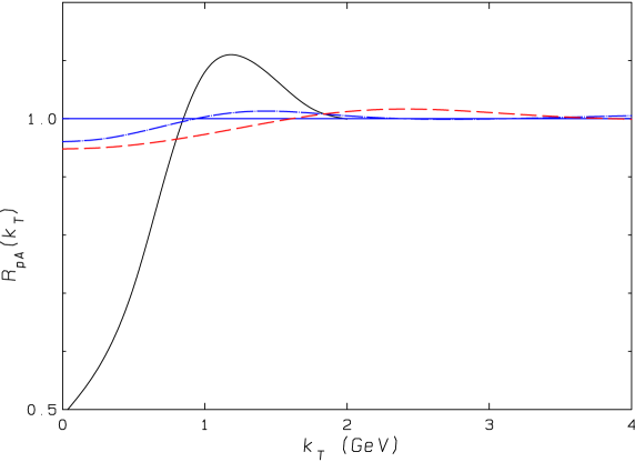
Figure 4: McLerran-Venugopalan model: $R_{pA}$ as a function of $k_{\bot}$. Solid curve for $M=2$ GeV and fixed $z=0.7$; dashed (dot-dashed) curve for$M=4(2)$ GeV and $y_{\gamma}=3$.

In order to set the reference we give results based on the McLerran-Venugopalan model [8] as described in Sec. 3, when using $\phi_{G}^{MV}$ of (26). Instead of explicitly taking the scale (17) we fix the values at $\vec{b}=0$ by $Q^{MV}_{s,A}=1$ GeV for $A=200$, and $Q_{s,p}=1/A^{1/6}$ GeV $\simeq 0.41$ GeV for the proton target, respectively.

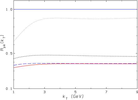
Figure 5: BFKL-saturation model: $R_{pA}$ as a function of $k_{\bot}$ for different values of $y_{\gamma}$ and for $M=2$ GeV: dotted ($y_{\gamma}=0.5$), short-dashed ($y_{\gamma}=1.5$), long-dashed ($y_{\gamma}=3.0$). Solid curve for $M=4$ GeV and $y_{\gamma}=3$.

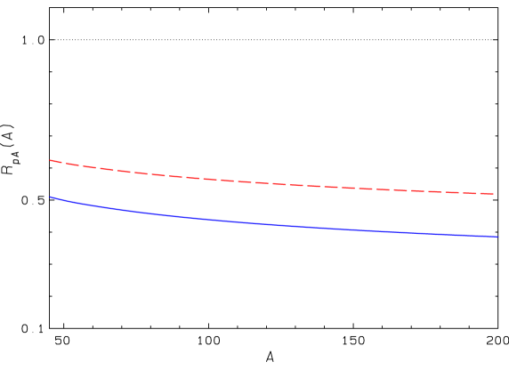
Figure 6: BFKL-saturation model: $R_{pA}$ as a function of $A$ for $k_{\bot}=5$ GeV, $y_{\gamma}=3$ and $M=2$ GeV (solid curve). Dashed curve corresponds to $A^{-{\lambda_{0}/3}}$.

For small photon rapidities, $y_{\gamma}\simeq 0$, and dilepton masses of $M=2-4$ GeV the ratio $R_{pA}$ of (40) as a function of $k_{\bot}$ is essentially $R_{pA}=1$. This is easy to see from (8): small values of $z\leq 0.05$ imply that $H$ of (33) is approximated by $H\approx q^{2}_{\bot}/(k^{2}_{\bot}+\eta^{2})$. Because of (20) it follows that $R_{pA}\approx A^{-1/3}(Q^{MV}_{s,A}/Q_{s,p})^{2}\simeq 1$. For comparison with the prediction for evolved gluons we also consider larger values of $y_{\gamma}$, e.g. $y_{\gamma}=3$, in this model. The results for $R_{pA}$ are plotted in Fig. 4 for two values of $M=2$ and $M=4$ GeV, respectively. A very small suppression, $R_{pA}\geq 0.95$, is observed for $k_{\bot}\leq 1-2$ GeV. Keeping, however, the value of $z$ fixed and large, e.g. $z=0.7$, a significant Cronin type pattern for the transverse Drell-Yan spectrum is observed (solid curve in Fig. 4): shadowing for $k_{\bot}\leq 1$ GeV, and enhancement above. This confirms the results first presented in [27]. However, we have to keep in mind that this model is only reliable, when $k_{\bot}>Q^{MV}_{s}$.

In order to obtain results at large photon rapidities based on the BFKL evolution in the presence of saturation we pragmatically have to choose the $Y$ dependence of the scale, instead of the one given by (27). As already discussed in Sec. 3 we take the one compatible with phenomenology, following [46],

$$Q^{2}_{s}(\vec{b}=0,Y=y_{\gamma})=(Q^{MV}_{s})^{2}\exp(\lambda_{GBW}\,y_{\gamma}),\,\,\lambda_{GBW}=0.3\,\,.$$ (42)

In accordance with the discussion in Sec. 5.1 significant shadowing is obtained, as shown in Fig. 5 as a function of $k_{\bot}$, especially when the dileptons are produced rather forward, e.g. with $y_{\gamma}=3$. Similar results, however, for $k_{\bot}$-integrated dilepton rates are presented in [31].

When $k_{\bot}>>Q_{s}(\vec{b}=0,Y)$ the ratio $R_{pA}$ becomes essentially independent on the transverse momentum.

Finally, we numerically check the statement in (37) concerning the $A$ dependence of the $\gamma^{*}$ cross section ratio for central collsions. An example is plotted in Fig. 6, indicating that indeed the anomalous $A$ dependence is to be expected for large nuclei, with the consequence of strong (leading twist) shadowing of photons/dileptons, when produced in the forward direction of $pA$, or $dA$ collisions.

Acknowledgments

The authors gratefully acknowledge helpful discussions with Francois Gelis and Jamal Jalilian-Marian. R. B. is supported, in part, by DFG, contract FOR 329/2-1, and A. M. is supported, in part, by the US Department of Energy.

Appendix A

In this appendix we relate the $k_{\bot}$-representation of the $\gamma^{*}$ production cross section, Eq.(8), to its impact parameter representation [26, 27, 28]. In order to go from $\vec{k}_{\bot}$ to the conjugate coordinate $\vec{x}_{\bot}$, we introduce the Fourier transform of the propagator [38],

$$\frac{\vec{\epsilon}^{~{}\lambda}_{\bot}\cdot\vec{k}_{\bot}}{k_{\bot}^{2}+\eta^{2}} = -i\int\frac{d^{2}x_{\bot}}{2\pi}\left(\vec{\epsilon}^{~{}\lambda}_{\bot}\cdot\vec{\nabla}_{x_{\bot}}e^{i\vec{k}_{\bot}\cdot\vec{x}_{\bot}}\right)K_{0}(\eta x_{\bot})$$ (A.1)

$$= -i\eta\int\frac{d^{2}x_{\bot}}{2\pi}e^{i\vec{k}_{\bot}\cdot\vec{x}_{\bot}}\frac{\vec{\epsilon}^{~{}\lambda}_{\bot}\cdot\vec{x}_{\bot}}{x_{\bot}}K_{1}(\eta x_{\bot}),$$ (A.2)

with $x_{\bot}=|\vec{x}_{\bot}|$ and $K_{i}$ the Bessel functions of the second kind, $K_{1}(z)=-\frac{d}{dz}K_{0}(z)$.

The square of the radiation amplitude (4) is expressed by

$$\sum_{\lambda} \left|\frac{\vec{\epsilon}^{~{}\lambda}_{\bot}\cdot\vec{k}_{\bot}}{k_{\bot}^{~{}2}+\eta^{2}}-\frac{\vec{\epsilon}^{~{}\lambda}_{\bot}\cdot\vec{k}_{\bot}^{~{}\prime}}{k_{\bot}^{~{}\prime 2}+\eta^{2}}\right|^{2}=$$

$$\int\frac{d^{2}x_{\bot}d^{2}y_{\bot}}{(2\pi)^{2}}e^{i\vec{k}_{\bot}\cdot(\vec{x}_{\bot}-\vec{y}_{\bot})}\,\eta^{2}\frac{\vec{x}_{\bot}\cdot\vec{y}_{\bot}}{x_{\bot}y_{\bot}}K_{1}(\eta x_{\bot})K_{1}(\eta y_{\bot})$$

$$\times\left[\left(1-e^{-iz\vec{q}_{\bot}\cdot x_{\bot}}\right)+\left(1-e^{+iz\vec{q}_{\bot}\cdot\vec{y}_{\bot}}\right)-\left(1-e^{-iz\vec{q}_{\bot}\cdot(\vec{x}_{\bot}-\vec{y}_{\bot})}\right)\right]$$

Following [27], we introduce the transverse photon wave function for $q\rightarrow\gamma^{*}q$, $~{}\psi^{\lambda}_{\gamma q}(z,x_{\bot},\eta)$, with

$$\sum_{\lambda}\psi^{\lambda^{*}}_{\gamma q}(z,\vec{x}_{\bot},\eta)\psi^{\lambda}_{\gamma q}(z,\vec{y}_{\bot},\eta)=$$

$$\frac{\alpha_{em}}{2\pi^{2}}[1+(1-z)^{2}]\,\eta^{2}\,\frac{\vec{x}_{\bot}\cdot\vec{y}_{\bot}}{x_{\bot}y_{\bot}}K_{1}(\eta x_{\bot})K_{1}(\eta y_{\bot})\,.$$ (A.4)

Inserting (15) for the unintegrated gluon function $\phi_{G}$, namely

$$\int\frac{d^{2}q_{\bot}}{q^{2}_{\bot}}\phi_{G}(\vec{b},\vec{q}_{\bot},Y)\left(1-e^{-iz\vec{q}_{\bot}\cdot\vec{x}_{\bot}}\right)=\frac{N_{c}}{2\pi\alpha_{s}}N(\vec{b},z\vec{x}_{\bot},Y)\,,$$ (A.5)

into the $\gamma^{*}$ cross section (8) we finally obtain, together with (Appendix A) the impact parameter representation of the $\gamma^{*}$ cross section [27],

$$\frac{d\sigma^{qA\rightarrow\gamma^{*}X}}{d^{2}bd^{2}k_{\bot}d\ln z}=\int\frac{d^{2}x_{\bot}d^{2}y_{\bot}}{(2\pi)^{2}}e^{i\vec{k}_{\bot}\cdot(\vec{x}_{\bot}-\vec{y}_{\bot})}$$ (A.6)

$$\times\sum_{\lambda}\psi^{\lambda^{*}}_{\gamma q}(z,\vec{x}_{\bot},\eta)\psi^{\lambda}_{\gamma q}(z,\vec{y}_{\bot},\eta)\left[N(\vec{b},z\vec{x}_{\bot},Y)+N(\vec{b},z\vec{y}_{\bot},Y)-N(\vec{b},z(\vec{x}_{\bot}-\vec{y}_{\bot}),Y)\right].$$

In the $q\bar{q}$-dipole approximation for scattering off a nucleus $A$, the amplitude $N=1-S$, where

$$S(\vec{b},\vec{x}_{\bot},Y)=\exp[-\frac{1}{2}\sigma_{q\bar{q}}(\vec{b},\vec{x}_{\bot},Y)]=\exp[-x^{~{}2}_{\bot}\bar{Q}^{~{}2}_{s}(\vec{b})/4]\,,$$ (A.7)

is expressed by the $\sigma_{q\bar{q}}$ cross section or by the saturation scale $\bar{Q}^{~{}2}_{s}(\vec{b})=\frac{C_{F}}{N_{c}}Q^{2}_{s}(\vec{b})$ given in (17)[37, 38].

Let us add two useful relations:

• The limiting case for real photon emission, $\eta\rightarrow 0$, is obtained from (A.4) by

  $$\sum_{\lambda}\psi^{\lambda^{*}}_{\gamma q}(z,\vec{x}_{\bot})\psi^{\lambda}_{\gamma q}(z,\vec{y}_{\bot})\rightarrow\frac{\alpha_{em}}{2\pi^{2}}[1+(1-z)^{2}]\frac{\vec{x}_{\bot}\cdot\vec{y}_{\bot}}{x^{2}_{\bot}y^{2}_{\bot}}\,.$$ (A.8)

• Via crossing from $q\rightarrow q\gamma^{*}(M)$ into $\gamma^{*}(Q)\rightarrow q\bar{q}$ the DIS cross section is obtained from the expression (A.6) by the substitutions

  $$z\rightarrow\frac{1}{1-\alpha},\,\,{\rm i.e.}\,\,\frac{1+(1-z)^{2}}{z^{2}}\rightarrow(1-\alpha)^{2}+\alpha^{2},$$ (A.9)

  and

  $$K_{1}(\eta x_{\bot})=K_{1}\left(\sqrt{(1-z)M^{2}x^{2}_{\bot}}\right)\rightarrow K_{1}\left(\sqrt{\alpha(1-\alpha)Q^{2}{\bar{x}}^{2}_{\bot}}\right),$$ (A.10)

  where the $q\bar{q}$ separation is given by $\bar{x}_{\bot}=\frac{x_{\bot}}{1-\alpha}=zx_{\bot}$, such that

  $$N(\vec{b},z\vec{x}_{\bot},Y)\rightarrow N(\vec{b},\vec{\bar{x}}_{\bot},Y)\,.$$ (A.11)

  The explicit expressions for deep inelastic scattering may be found in [26, 37].

Appendix B

Here we give some details on the behaviour of the leading order (LO) cross section for real and isolated photons produced via the process $qA\rightarrow\gamma X$ [30]. The photon takes away a large transverse momentum $k_{\bot},k_{\bot}\gg Q_{s}$, opposite to a recoil quark jet.

The differential cross section for real photons, $M^{2}=0$, in the $k_{\bot}$-factorized form reads (see Eq. (8)),

$$\frac{d\sigma}{d^{2}bd^{2}k_{\bot}d\ln z}=\frac{\alpha_{em}\alpha_{s}}{\pi N_{c}}\frac{1+(1-z)^{2}}{k^{2}_{\bot}}\int d^{2}q_{\bot}\frac{\phi_{G}(\vec{b},\vec{q}_{\bot},Y)}{[\vec{q}_{\bot}-\vec{k}_{\bot}/z]^{2}}.$$ (B.1)

Assuming $k_{\bot}\gg z\vec{q}_{\bot}$, i.e. such that collinear quark-isolated photon configurations are suppressed, we may write (B.1) as

$$\frac{d\sigma}{d^{2}k_{\bot}d\ln z}=\frac{\alpha_{em}\alpha_{s}}{N_{c}}\frac{z^{2}[1+(1-z)^{2}]}{k^{4}_{\bot}}xG_{A}\left(x=\frac{x^{2}_{T}}{z(1-z)},Q^{2}=k^{2}_{\bot}\right),$$ (B.2)

where $xG_{A}$ is the gluon distribution in the nucleus $A$,

$$xG_{A}(x,k^{2}_{\bot})=\int^{O(k_{\bot})}\frac{d^{2}q_{\bot}}{\pi}\int d^{2}b\phi_{G}(\vec{b},\vec{q}_{\bot},Y).$$ (B.3)

in agreement with (LABEL:(4)). For real photons $x_{T}=k_{\bot}/\sqrt{s}$ and $z=x_{\bot}\exp{y_{\gamma}}$, such that the $x$ value in the gluon is decreasing with increasing photon rapidity $y_{\gamma}$. The expression (B.2) is the same as derived from the hard LO pQCD $2\rightarrow 2$ Compton process $qG\rightarrow\gamma q$ for production of isolated photons at large $k_{\bot}$ [36]: indeed the corresponding hard cross section is given by

$$\frac{d\sigma}{d\hat{t}}^{qG\rightarrow\gamma q} = \frac{\pi\alpha_{em}\alpha_{s}}{N_{c}}\,\frac{1}{\hat{s}^{~{}2}}\left[-\frac{\hat{s}}{\hat{t}}-\frac{\hat{t}}{\hat{s}}\right]$$ (B.4)

$$= \frac{\pi\alpha_{em}\alpha_{s}}{N_{c}}\,\frac{z^{2}(1-z)[1+(1-z)^{2}]}{k_{\bot}^{4}},$$

since $\hat{s}=\frac{k^{2}_{\bot}}{z(1-z)},\,\hat{t}=-k^{2}_{\bot}/z$. After folding (B.4) into the expression for $qA\rightarrow\gamma X$ with the help of the gluon function $xG_{A}$ in the nucleus $A$ and performing the integration over the recoiling quark leads to (B.2).

Using (LABEL:(III.1)), we relate the gluon distribution $\phi_{G}$ to the dipole amplitude $N_{q\bar{q}}$ in the quasi-classical approximation [8]. With (A.7) one obtains,

$$\phi_{G}(\vec{b},\vec{q}_{\bot},Y)=\frac{N_{c}}{(2\pi)^{3}\alpha_{s}}\int d^{2}x_{\bot}e^{i\vec{q}_{\bot}\cdot\vec{x}_{\bot}}\vec{\nabla}^{2}_{x_{\bot}}[1-\exp(-x^{2}_{\bot}\bar{Q}^{2}_{s}/4)],$$ (B.5)

with the scale given by (17). At very large $q_{\bot}\gg Q_{s}$ one finds,

$$\phi_{G}^{\rm{LO}}(\vec{b},\vec{q}_{\bot},Y)=\rho T(b)\,\frac{\alpha_{s}N_{c}C_{F}}{q^{~{}2}_{\bot}}\,.$$ (B.6)

This is derived by using the LO gluon distribution,

$$xG^{{\rm LO}}(x,1/x^{2}_{\bot})=\frac{C_{F}N_{c}\alpha_{s}}{\pi}\ln\frac{1}{x^{2}_{\bot}\Lambda^{2}},$$ (B.7)

and thus

$$N^{\rm{LO}}(\vec{b},\vec{x}_{\bot},Y)=x^{2}_{\bot}\bar{Q}^{~{}2}_{s}(\vec{b})/4=\frac{C_{F}\alpha^{2}_{s}}{2}\rho T(b)x^{2}_{\bot}\ln\frac{1}{x^{2}_{\bot}\Lambda^{2}}\,.$$ (B.8)

(B.6) follows by using [48]

$$\int\frac{d^{2}x_{\bot}}{(2\pi)^{2}}e^{i\vec{q}_{\bot}\cdot\vec{x}_{\bot}}\ln\left(\frac{1}{x^{2}_{\bot}\Lambda^{2}}\right)=\frac{1}{\pi q^{2}_{\bot}},$$ (B.9)

valid for $\vec{q}_{\bot}\not=0$. Since

$$\int\phi^{{\rm LO}}_{G}(\vec{b},\vec{q}_{\bot},Y)d^{2}b=A\frac{\alpha_{s}C_{F}N_{c}}{\pi}\frac{1}{q^{2}_{\bot}},$$ (B.10)

the LO factorized result for the gluon in nucleus $A$,

$$xG^{{\rm LO}}_{A}(x,k^{2}_{\bot})\simeq A\frac{(N^{2}_{c}-1)\alpha_{s}}{2\pi}\ln\frac{k^{2}_{\bot}}{\Lambda^{2}}=AxG^{{\rm LO}}(x,k^{2}_{\bot}),$$ (B.11)

in terms of the ${\rm LO}$ gluon in the nucleon, is finally obtained.

Appendix C

In this appendix we extensively discuss in more general terms the relationship between the $k_{\bot}$-factorization, which has been used in the previous sections and the usual QCD factorization [36] involving local gauge invariant operators which appear in a Wilson operator product expansion. As in Appendix B, where we investigate this relationship for large $k_{\bot}>>Q_{s}$ in LO pQCD, we concentrate explicitly on the case of real photon production.

C.1 The forms of factorization

We restrict here our discussion to the scaling region where the hard scale is above, but not too far above, the saturation region. When the hard scale is below the saturation momentum neither $k_{\bot}$-factorization nor the usual QCD factorization is applicable as higher twist terms are coherent with leading twist terms and all terms must be considered together. While it does make sense to talk of a gluon distribution which has reached saturation, that distribution does not appear simply in factorization formulae. When the hard scale is very large and outside the scaling region $k_{\bot}$-factorization may still be useful, but the issues are more straightforward than in the scaling region.

We write generically a dimensionless observable in the $k_{\bot}$-factorized form

$$\sigma(\vec{Q},Y)=\int\frac{d^{2}q_{\bot}}{\pi q^{2}_{\bot}}\,H(\vec{q}_{\bot},\vec{Q})\,\phi_{G}(\vec{q}_{\bot},Y)\,,$$ (C.1)

and in the QCD factorization form

$$\sigma(\vec{Q},Y)=\frac{1}{Q^{2}}\int^{\infty}_{0}dy\,\tilde{H}(y)\,xG(\vec{Q},Y-y)\,,$$ (C.2)

where $Q$ is the hard scale of the reaction, $H$ is the hard part in the $k_{\bot}$-factorized form, and $\tilde{H}$ the hard part in the usual factorization. Here, and in the following, we suppress writting explicitly the dependence on the impact parameter $\vec{b}_{\bot}$. We suppose that the hard part in the $k_{\bot}$-factorized expression is not too nonlocal in rapidity while we cannot suppose such is the case for $\tilde{H}$. Finally the coupling in $H$ and $\tilde{H}$ should be taken at the hard scale $Q$. In our example of direct photon production the hard scale $Q$ becomes the transverse momentum, $k_{\bot}$, of the photon, while

$$\sigma(\vec{k}_{\bot},Y)\equiv\sigma(\vec{b}_{\bot},\vec{k}_{\bot},Y)=\frac{k^{~{}2}_{\bot}d\sigma}{d^{2}b_{\bot}d^{2}k_{\bot}d\ln z}\,,$$ (C.3)

and (c.f. (B.1))

$$H(\vec{q}_{\bot},\vec{k}_{\bot})=\frac{\alpha_{em}\alpha_{s}}{N_{c}}\,[1+(1-z)^{2}]\frac{q^{~{}2}_{\bot}}{(\vec{q}_{\bot}-\vec{k}_{\bot}/z)^{2}}\,.$$ (C.4)

In the scaling region we approximate $\phi_{G}$ and $xG$, respectively, from (28) by neglecting in the following possible constants under the logarithms. We write it in the form

$$\phi_{G}(\vec{q}_{\bot},Y)=\frac{C}{\alpha_{s}}\left(\frac{Q^{2}_{s}(Y)}{q^{2}_{\bot}}\right)^{1-\lambda_{0}}\,\ln(q^{2}_{\bot}/Q^{2}_{s}(Y))\,,$$ (C.5)

and

$$xG(Q,Y)=\frac{{\tilde{C}}Q^{2}}{\alpha_{s}}\left(\frac{Q^{2}_{s}(Y)}{Q^{2}}\right)^{1-\lambda_{0}}\,\ln(Q^{2}/Q^{2}_{s}(Y))\,.$$ (C.6)

In this region the normalizing factors $C$ and ${\tilde{C}}$ are not necessarily the same, and actually we have not been able to relate them.

C.2 The renormalization group

In this section we show that (C.6) obeys the renormalization group equation. In showing this we shall find a relation which will be crucial in relating $H$ and $\tilde{H}$, which appear in (C.1) and (C.2). Now in BFKL dynamics there are two alternate forms for $xG$,

$$xG(Q,Y)=\int\frac{dn}{2\pi i}A_{n}\,e^{\gamma_{n}\ln Q^{2}/\mu^{2}+(n-1)Y}\,,$$ (C.7)

and (c.f. (21))

$$xG(Q,Y)=\int\frac{d\lambda}{2\pi i}B_{\lambda}\,e^{2\bar{\alpha}\chi(\lambda)Y+\lambda\ln Q^{2}/\mu^{2}}\,,$$ (C.8)

where the scale $\mu$ is introduced to create dimensionless quantities, but $xG$ does not depend on $\mu$. The integral in (C.7) goes parallel to the imaginary axis with $Re(n)$ to the right of all singularities of $\gamma_{n}$ and $A_{n}$ in $n$. As discussed in Sec. 3, Eq. (C.8) is, of course, not a perfectly correct representation of BFKL dynamics in the presence of saturation, nevertheless the aspects of (C.8), which we use remain true even when the BFKL equation [11] is replaced by the Kovchegov equation [44].

In the scaling region the integrals in (C.7) and (C.8) are dominated by saddle points at $n=n_{0}$ and $\lambda=\lambda_{0}$, where $\lambda_{0}$ satisfies (29). Also for (C.7) and (C.8) to describe the same function it must be true that

$$n-1=2\bar{\alpha}\chi(\gamma_{n})\,,$$ (C.9)

which determines $\gamma_{n}$, while at the saddle points

$$n_{0}-1=2\bar{\alpha}\chi(\lambda_{0})\,,$$ (C.10)

and

$$\lambda_{0}=\gamma_{n_{0}}\,.$$ (C.11)

The renormalization group equation [36] is

$$Q^{2}\frac{\partial}{\partial Q^{2}}xG(Q,Y)=\int^{\infty}_{0}dy\,\gamma(y)\,xG(Q,Y-y),$$ (C.12)

with $\gamma(y)$ the gluon anomalous dimension

$$\gamma(y)=\int\frac{dn}{2\pi i}\gamma_{n}\,e^{(n-1)y}\,.$$ (C.13)

Using (C.6) along with the result (27),

$$Q^{2}_{s}(y)\simeq\frac{\exp\left\{\frac{2\bar{\alpha}\chi(\lambda_{0})}{1-\lambda_{0}}\,y\right\}}{[\alpha_{s}y]^{\frac{3}{2(1-\lambda_{0})}}}\,,$$ (C.14)

it is straight forward to get

$$xG(Q,Y-y)=xG(Q,Y)\,e^{-2\bar{\alpha}\chi(\lambda_{0})y}\left[1+\frac{\frac{2\bar{\alpha}\chi(\lambda_{0})}{1-\lambda_{0}}y}{\ln(Q^{2}/Q^{2}_{s}(y))}\right]\,,$$ (C.15)

so long as $y/Y\ll 1$. Using (C.6) on the left hand side of (C.12), and (C.15) on the right hand side one easily sees that (C.12) is satisfied if

$$\lambda_{0}=\int^{\infty}_{0}dy\,e^{-2\bar{\alpha}\chi(\lambda_{0})y}\,\gamma(y)\,,$$ (C.16)

and

$$1=\frac{2\bar{\alpha}\chi(\lambda_{0})}{1-\lambda_{0}}\int^{\infty}_{0}dy\,y\,\gamma(y)\,e^{-2\bar{\alpha}\chi(\lambda_{0})y}$$ (C.17)

are both true. Eq.(C.16) follows from (C.10), (C.11) and (C.13). Eq.(C.17) can be written as

$$1=-\frac{2\bar{\alpha}\chi(\lambda_{0})}{1-\lambda_{0}}\,\frac{d}{dn}\gamma_{n}\Bigg{|}_{n=n_{0}},$$ (C.18)

which requires the inverse representation of (C.13). The validity of (C.18) then follows from differentiating (C.9) with respect to $n$ and using (29).

C.3 The relationship between $k_{\bot}$-factorization and QCD factorization

We now reach the main topic of this section, namely the relationship between the two forms of factorization exhibited in (C.1) and (C.2). We begin with (C.1) and insert (C.5) for $\phi_{G}$. Thus

$$\sigma(\vec{Q},Y)=\int\frac{d^{2}q_{\bot}}{\pi q^{2}_{\bot}}\,H(\vec{q}_{\bot},\vec{Q})\,\frac{C}{\alpha_{s}}\left(\frac{Q^{2}_{s}(Y)}{q^{2}_{\bot}}\right)^{1-\lambda_{0}}\,\ln(q^{2}_{\bot}/Q^{2}_{s}(Y))\,.$$ (C.19)

Using (C.6) we arrive at

$$\sigma(\vec{Q},Y)=xG(Q,Y)\frac{1}{Q^{2}}\frac{C}{{\tilde{C}}}\,\int\frac{d^{2}q_{\bot}}{\pi q^{2}_{\bot}}\,H(\vec{q}_{\bot},\vec{Q})\left(\frac{Q^{2}}{q^{2}_{\bot}}\right)^{1-\lambda_{0}}\,\left[1+\frac{\ln(q^{2}_{\bot}/Q^{2})}{\ln(Q^{2}/Q^{2}_{s}(Y))}\right]\,.$$ (C.20)

Now we may rewrite, using (C.15) , QCD factorization as given in (C.2) as

$$\sigma(\vec{Q},Y)=xG(Q,Y)\frac{1}{Q^{2}}\int^{\infty}_{0}dy\tilde{H}(y)\,e^{-2\bar{\alpha}\chi(\lambda_{0})y}\,\left[1+\frac{\frac{2\bar{\alpha}\chi(\lambda_{0})}{1-\lambda_{0}}y}{\ln(Q^{2}/Q^{2}_{s}(Y))}\right]\,.$$ (C.21)

Using (C.10) one can write (C.21) as

$$\sigma(\vec{Q},Y)=xG(Q,Y)\frac{1}{Q^{2}}\left[\tilde{H}_{n}-\frac{\frac{n-1}{1-\lambda_{0}}\frac{\partial}{\partial n}}{\ln(Q^{2}/Q^{2}_{s}(Y))}\tilde{H}_{n}\right]\Bigg{|}_{n=n_{0}}\,,$$ (C.22)

with, of course,

$$\tilde{H}_{n}=\int^{\infty}_{0}dy\,{\tilde{H}}(y)\,e^{-(n-1)y}\,.$$ (C.23)

Comparing (C.20) and (C.22) it is easy to see that they are equivalent if

$$\tilde{H}_{n_{0}}=\frac{C}{{\tilde{C}}}\int\frac{d^{2}q_{\bot}}{\pi q^{2}_{\bot}}\left(\frac{Q^{2}}{q^{2}_{\bot}}\right)^{1-\lambda_{0}}H(\vec{q}_{\bot},\vec{Q})\,,$$ (C.24)

and

$$-\frac{n_{0}-1}{1-\lambda_{0}}\frac{\partial}{\partial n_{0}}\tilde{H}_{n_{0}}=\frac{C}{{\tilde{C}}}\int\frac{d^{2}q_{\bot}}{\pi q^{2}_{\bot}}\left(\frac{Q^{2}}{q^{2}_{\bot}}\right)^{1-\lambda_{0}}\ln(q^{2}_{\bot}/Q^{2})H(\vec{q}_{\bot},\vec{Q})\,,$$ (C.25)

are satisfied. Eq. (C.24) is easy to satisfy, if we choose to define $\tilde{H}(y)$ by

$$\tilde{H}(y)=\int\,\frac{dn}{2\pi i}\,e^{(n-1)y}\tilde{H}_{n}\,,$$ (C.26)

and with (C.11)

$$\tilde{H}_{n}=\frac{C}{{\tilde{C}}}\int\frac{d^{2}q_{\bot}}{\pi q^{2}_{\bot}}\left(\frac{Q^{2}}{q^{2}_{\bot}}\right)^{1-\gamma_{n}}H(\vec{q}_{\bot},\vec{Q}).$$ (C.27)

Then it is straight forward to see that (C.24) is satisfied while (C.25) follows by using

$$\frac{d\gamma_{n}}{dn}\Bigg{|}_{n=n_{0}}=-\frac{(1-\lambda_{0})}{n_{0}-1}\,,$$ (C.28)

which, after using (C.10), is the same as (C.18).

Thus we see that $k_{\bot}$-factorization as expressed in (C.1) leads to QCD factorization, as expressed in (C.2), with $\tilde{H}(y)$ defined by (C.26) and (C.27). While $H(\vec{q}_{\bot},\vec{Q})$ is a lowest order expression, $\tilde{H}(y)$ is determined in terms of a resummation dictated by (C.26) and (C.27) and cannot be limited to its lowest order term. The simplicity of $k_{\bot}$-factorization is that all resummations are put into $\phi_{G}$ with $H$ remaining a relatively simple quantity, that is the hard part defining the reaction is more visible in $k_{\bot}$-factorization than in QCD factorization. We remark that including a common additional constant under the logarithms in (C.5) and (C.6), respectively, does not destroy the derivation given above. It remains a challenge to understand how to extend $k_{\bot}$-factorization beyond a leading logarithmic formalism.

References

• [1] A. Accardi et al., “Hard probes in heavy ion collisions at the LHC: Jet physics,” arXiv:hep-ph/0310274.
• [2] T. Ludlam and L. McLerran, Phys. Today 56N10 (2003) 48.
• [3] Recent overviews: U. A. Wiedemann, arXiv:hep-ph/0402251; I. Vitev, arXiv:hep-ph/0403089; D. d’Enterria [PHENIX Collaboration], arXiv:nucl-ex/0401001.
• [4] B. B. Back et al. [PHOBOS Collaboration], Phys. Rev. Lett.  91 (2003) 072302 [arXiv:nucl-ex/0306025]; S. S. Adler et al. [PHENIX Collaboration], Phys. Rev. Lett.  91 (2003) 072303 [arXiv:nucl-ex/0306021]; J. Adams et al. [STAR Collaboration], Phys. Rev. Lett.  91 (2003) 072304 [arXiv:nucl-ex/0306024]; I. Arsene et al. [BRAHMS Collaboration], Phys. Rev. Lett.  91 (2003) 072305 [arXiv:nucl-ex/0307003].
• [5] R. Debbe [BRAHMS Collaboration], talk given at the APS DNP Meeting at Tucson, AZ, October, 2003; I. Arsene [BRAHMS Collaboration], arXiv:nucl-ex/0401025.
• [6] L. V. Gribov, E. M. Levin and M. G. Ryskin, Phys. Rept.  100, 1 (1983).
• [7] A. H. Mueller and J. w. Qiu, Nucl. Phys. B 268, 427 (1986); J. P. Blaizot and A. H. Mueller, Nucl. Phys. B 289, 847 (1987).
• [8] L. D. McLerran and R. Venugopalan, Phys. Rev. D 49, 2233 (1994) [arXiv:hep-ph/9309289], Phys. Rev. D 49, 3352 (1994) [arXiv:hep-ph/9311205], Phys. Rev. D 50, 2225 (1994) [arXiv:hep-ph/9402335], Phys. Rev. D 59, 094002 (1999) [arXiv:hep-ph/9809427]. A. Ayala, J. Jalilian-Marian, L. D. McLerran and R. Venugopalan, Phys. Rev. D 53, 458 (1996) [arXiv:hep-ph/9508302]; Y. V. Kovchegov, Phys. Rev. D 54, 5463 (1996) [arXiv:hep-ph/9605446].
• [9] Recent reviews: E. Iancu, A. Leonidov and L. McLerran, arXiv:hep-ph/0202270; A. H. Mueller, Nucl. Phys. A 715 (2003) 20 [arXiv:hep-ph/0208278]; E. Iancu and R. Venugopalan, arXiv:hep-ph/0303204; L. McLerran, arXiv:hep-ph/0402137.
• [10] See also: A. Dumitru and J. Jalilian-Marian, Phys. Lett. B 547 (2002) 15 [arXiv:hep-ph/0111357]; Phys. Rev. Lett.  89 (2002) 022301 [arXiv:hep-ph/0204028]; F. Gelis and J. Jalilian-Marian, Phys. Rev. D 67 (2003) 074019 [arXiv:hep-ph/0211363].
• [11] E. A. Kuraev, L. N. Lipatov and V. S. Fadin, Sov. Phys. JETP 45, 199 (1977) [Zh. Eksp. Teor. Fiz.  72, 377 (1977)]. I. I. Balitsky and L. N. Lipatov, Sov. J. Nucl. Phys.  28, 822 (1978) [Yad. Fiz.  28, 1597 (1978)].
• [12] F. Arleo et al., “Photon physics in heavy ion collisions at the LHC,” arXiv:hep-ph/0311131.
• [13] G. Fai, J. Qiu and X. Zhang, arXiv:hep-ph/0403126.
• [14] Y. V. Kovchegov and A. H. Mueller, Nucl. Phys. B 529, 451 (1998) [arXiv:hep-ph/9802440].
• [15] Y. V. Kovchegov, Phys. Rev. D 55, 5445 (1997) [arXiv:hep-ph/9701229].
• [16] Y. V. Kovchegov, Phys. Rev. D 64, 114016 (2001) [Erratum-ibid. D 68, 039901 (2003)] [arXiv:hep-ph/0107256].
• [17] B. Z. Kopeliovich, J. Nemchik, A. Schafer and A. V. Tarasov, Phys. Rev. Lett.  88, 232303 (2002) [arXiv:hep-ph/0201010].
• [18] D. Kharzeev, E. Levin and L. McLerran, Phys. Lett. B 561, 93 (2003) [arXiv:hep-ph/0210332].
• [19] R. Baier, A. Kovner and U. A. Wiedemann, Phys. Rev. D 68, 054009 (2003) [arXiv:hep-ph/0305265].
• [20] J. L. Albacete, N. Armesto, A. Kovner, C. A. Salgado and U. A. Wiedemann, Phys. Rev. Lett.  92 (2004) 082001 [arXiv:hep-ph/0307179].
• [21] D. Kharzeev, Y. V. Kovchegov and K. Tuchin, Phys. Rev. D 68, 094013 (2003) [arXiv:hep-ph/0307037]; and arXiv: hep-ph/0405045.
• [22] J. Jalilian-Marian, Y. Nara and R. Venugopalan, Phys. Lett. B 577, 54 (2003) [arXiv:nucl-th/0307022].
• [23] J. P. Blaizot, F. Gelis and R. Venugopalan, arXiv:hep-ph/0402256; J. P. Blaizot, F. Gelis and R. Venugopalan, arXiv:hep-ph/0402257.
• [24] J. Jalilian-Marian, arXiv:nucl-th/0402080.
• [25] E. Iancu, K. Itakura and D. N. Triantafyllopoulos, arXiv:hep-ph/0403103.
• [26] S. J. Brodsky, A. Hebecker and E. Quack, Phys. Rev. D 55 (1997) 2584 [arXiv:hep-ph/9609384].
• [27] B. Z. Kopeliovich, A. V. Tarasov and A. Schafer, Phys. Rev. C 59, 1609 (1999) [arXiv:hep-ph/9808378].
• [28] B. Z. Kopeliovich, J. Raufeisen and A. V. Tarasov, arXiv:hep-ph/0104155; B. Z. Kopeliovich, J. Raufeisen, A. V. Tarasov and M. B. Johnson, Phys. Rev. C 67 (2003) 014903 [arXiv:hep-ph/0110221]; B. Z. Kopeliovich, J. Raufeisen and A. V. Tarasov, Phys. Lett. B 503 (2001) 91 [arXiv:hep-ph/0012035]; J. Raufeisen, arXiv:hep-ph/0204096; J. Raufeisen, J. C. Peng and G. C. Nayak, Phys. Rev. D 66 (2002) 034024 [arXiv:hep-ph/0204095]; J. Raufeisen, arXiv:hep-ph/0204018.
• [29] F. Gelis and J. Jalilian-Marian, Phys. Rev. D 66 (2002) 094014 [arXiv:hep-ph/0208141].
• [30] F. Gelis and J. Jalilian-Marian, Phys. Rev. D 66 (2002) 014021 [arXiv:hep-ph/0205037].
• [31] J. Jalilian-Marian, arXiv:nucl-th/0402014.
• [32] A. H. Mueller and D. N. Triantafyllopoulos, Nucl. Phys. B 640, 331 (2002) [arXiv:hep-ph/0205167].
• [33] E. Iancu, K. Itakura and S. Munier, arXiv:hep-ph/0310338.
• [34] R. Baier, Y. L. Dokshitzer, A. H. Mueller, S. Peigne and D. Schiff, Nucl. Phys. B 484, 265 (1997) [arXiv:hep-ph/9608322].
• [35] R. Baier, Y. L. Dokshitzer, A. H. Mueller and D. Schiff, Nucl. Phys. B 531 (1998) 403 [arXiv:hep-ph/9804212].
• [36] R. K. Ellis, W. J. Stirling and B. R. Webber, Cambridge Monogr. Part. Phys. Nucl. Phys. Cosmol.  8 (1996) 1; and references therein.
• [37] A. H. Mueller, arXiv:hep-ph/0111244.
• [38] A. H. Mueller, Nucl. Phys. B 558 (1999) 285 [arXiv:hep-ph/9904404].
• [39] N. Armesto and M. A. Braun, Nucl. Phys. A 699 (2002) 320. N. Armesto and M. A. Braun, Eur. Phys. J. C 20 (2001) 517 [arXiv:hep-ph/0104038]. M. Braun, Eur. Phys. J. C 16 (2000) 337 [arXiv:hep-ph/0001268]; N. Armesto, arXiv:hep-ph/0311182.
• [40] Y. V. Kovchegov and K. Tuchin, Phys. Rev. D 65, 074026 (2002) [arXiv:hep-ph/0111362].
• [41] A. H. Mueller and B. Patel, Nucl. Phys. B 425 (1994) 471 [arXiv:hep-ph/9403256].
• [42] D. N. Triantafyllopoulos, Nucl. Phys. B 648, 293 (2003) [arXiv:hep-ph/0209121].
• [43] E. Iancu, K. Itakura and L. McLerran, Nucl. Phys. A 708, 327 (2002) [arXiv:hep-ph/0203137], E. Iancu, K. Itakura and L. McLerran, Nucl. Phys. A 724, 181 (2003) [arXiv:hep-ph/0212123].
• [44] I. Balitsky, Nucl. Phys. B 463, 99 (1996) [arXiv:hep-ph/9509348]; Y. V. Kovchegov, Phys. Rev. D 60, 034008 (1999) [arXiv:hep-ph/9901281]; Y. V. Kovchegov, Phys. Rev. D 61 (2000) 074018 [arXiv:hep-ph/9905214].
• [45] S. Munier and R. Peschanski, arXiv:hep-ph/0310357; Phys. Rev. Lett.  91 (2003) 232001 [arXiv:hep-ph/0309177].
• [46] K. Golec-Biernat and M. Wusthoff, Phys. Rev. D 59 (1999) 014017 [arXiv:hep-ph/9807513]; Phys. Rev. D 60 (1999) 114023 [arXiv:hep-ph/9903358]; J. Bartels, K. Golec-Biernat and H. Kowalski, Phys. Rev. D 66 (2002) 014001 [arXiv:hep-ph/0203258].
• [47] A. M. Stasto, K. Golec-Biernat and J. Kwiecinski, Phys. Rev. Lett.  86, 596 (2001) [arXiv:hep-ph/0007192].
• [48] Y. V. Kovchegov, Nucl. Phys. A 692 (2001) 557 [arXiv:hep-ph/0011252].