$Q$-ball Metamorphosis

Abstract

Flat directions in the minimal supersymmetric standard model are known to deform into non-topological solitons, $Q$-balls, which generally possess both baryon and lepton asymmetries. We investigate how $Q$-balls evolve if some of the constituent fields of the flat direction decay into light species. It is found that the $Q$-balls takes a new configuration whose energy per charge slightly increases due to the decay. Specifically, we show that all the stable $Q$-balls eventually transform into pure $B$-balls via the decay into neutrinos.

I introduction

Non-topological solitons, such as $Q$-balls Coleman:1985ki and $I$-balls Kasuya:2002zs , play important roles in the particle cosmology, partly because they are (quasi-)stable objects. Their stability comes from the conservation law. The $Q$-ball is composed of a complex scalar field with an $U(1)$ charge, the conservation of which enables the $Q$-ball to be stable or long-lived. Similarly, $I$-balls are composed of a real scalar field (or a complex scalar field in a nearly straight-line motion), whose dynamics conserve the adiabatic charge. Since we can only see either these objects in their final state or their decay products in the present universe, it is important to study their evolution during the course of the expanding universe.

The baryon asymmetry is one of the key observational results to uncover the history of the universe. Among many baryogenesis scenarios proposed so far, the mechanism proposed by Affleck and Dine Affleck:1984fy can be realized in the minimal extension of the standard model, that is, the minimal supersymmetric standard model (MSSM). The mechanism makes use of one of flat directions, along which there is no classical potential in the supersymmetric limit. Although the flat direction is parametrized by a set of chiral superfields, it is convenient and even sufficient in the usual situation to express it in terms of a single complex scalar field dubbed ‘Affleck-Dine (AD) field,’ $\Phi$, which generally has nonzero baryon and lepton charges. The dynamics of the AD field not only generates the desired baryon asymmetry, but allows non-topological solitons to be formed. The properties of $Q$-balls in the context of the AD mechanism have been extensively studied Kusenko:1997si ; Enqvist:1998en ; Kasuya:1999wu ; Kasuya:2000wx . $Q$-balls can be stable or unstable depending on the situation. Stable $Q$-balls can be dark matter Kusenko:1997si ; Kasuya:2000sc ; Kasuya:2001hg , which might solve the coincidence problem between the abundance of baryons and that of dark matter. Unstable but long-lived $Q$-balls can keep the baryon and lepton asymmetries stored inside them from being subject to the sphaleron effects. For instance, they can successfully generate both large lepton asymmetry and small baryon asymmetry Kawasaki:2002hq . It is even possible to realize the late-time baryon appearance after the relevant BBN epoch with use of $Q$-balls Ichikawa:2004pb . $I$-balls are also formed in the AD mechanism as an excited state of $Q$-balls.

In the examples mentioned above, the single-field parametrization is simple and valid. However, if we examine the evolution of $Q$-balls closely, we have to pay much more attention to the fact that the flat direction is actually composed of several scalar fields. Indeed, the slepton condensate always decays into a pair of neutrinos, while the squark condensate can decay into hadrons only if its energy per one baryon charge exceeds the nucleon or meson masses. Therefore, if a $Q$-ball has nonzero baryon and lepton asymmetries and its energy per unit charge is small enough, the leptonic component decays, leaving only the baryon asymmetry inside $Q$-balls (i.e., pure $B$-balls). However, since the $Q$-ball solution is obtained under the assumption that the $U(1)$ charge, $Q$, is conserved, it is not trivial how the $Q$-ball configuration changes during the course of the partial decay. Do $Q$-balls come apart? Or do they change their shape to satisfy the modified $Q$-ball solution? It is the purpose of this study to answer these questions.

In this paper, we investigate how $Q$-balls evolve if some of the constituent fields decay into lighter species. In the next section, we review the flat direction of the MSSM and the $Q$-ball solution. In section III we study the partial decay of $Q$-balls with a toy model of the flat direction. The results obtained there are confirmed with use of numerical calculation presented in section IV. Finally we give discussions and conclusions in section V.

II Preliminaries

In this section, first we explain how flat directions are expressed, paying particular attention to the single-field parametrization. Then we review the $Q$-ball solution relevant for the next section.

II.1 Flat directions

In the MSSM, there are many flat directions along which both the $D$-term and $F$-term potentials vanish at the classical level. The $D$-flat direction is labeled by a holomorphic gauge-invariant monomial, $X$. Most of $D$-flat directions can be also $F$-flat, simply due to a generation structure of the quark and lepton sector. Since it is easy to satisfy the $F$-flat condition, let us concentrate on the $D$-flat condition in the following. The $D$-flat direction, $X$, can be expressed as

$$X\equiv\prod_{i}^{N}\Phi_{i},$$ (1)

where $N$ superfields $\left\{\Phi_{i}\right\}$ constitute the flat direction $X$, and we have suppressed the gauge and family indices with the understanding that Latin letter $i$ contains all the information to label those constituents. When $X$ has a non-zero expectation value, each constituent field also takes a non-zero expectation value

$$\left\langle\Phi_{i}\right\rangle=\frac{\phi_{i}}{\sqrt{2}}e^{i\theta_{i}}.$$ (2)

Here each $\phi_{i}/\sqrt{2}$ is the absolute value of the expectation value $\left\langle\Phi_{i}\right\rangle$, and is related to every other due to the $D$-flat conditions:

$$\frac{1}{2}\sum_{A}\left(\sum_{ij}\Phi_{i}^{*}(T_{A})_{ij}\Phi_{j}\right)^{2}=0,$$ (3)

where $T_{A}$ are hermitian matrices representing the generators of the gauge algebra, and they are labeled with $A$. This condition can be usually satisfied if we take all $\phi_{i}$ equal: $\phi_{i}\equiv\phi/\sqrt{N}$. Note that $D$-flat condition dictates that all the amplitudes be equal, while the phases, $\theta_{i}$, remain to be arbitrary. In fact, it is necessary to know the pattern of baryon and lepton symmetry breaking, in order to identify the Nambu-Goldstone (NG) boson relevant for the AD mechanism. The situation becomes simple if the spontaneously broken symmetry coincides with the explicitly violated one. This is the case if the A-term is given by some powers of $X$. Then all $\theta_{i}$ become equivalent, and the NG boson can be identified with the average of $\theta_{i}$ Takahashi:2003db :

$$\theta\equiv\frac{1}{N}\sum_{i}\theta_{i},$$ (4)

where $\theta$ is orgthogonal to the NG mode corresponding to the spontaneously broken $U(1)$ gauge symmetry, that is, the linear combination of left isospin $T_{L3}$ and weak hypercharge $Y$. This is because $\sum_{i}T_{L3,i}=\sum_{i}Y_{i}=0$ by definition of the $D$-flat direction. Thus, the dynamics of the flat direction, $X$, can be well described by one complex scalar field, $\Phi$, which is defined as

$$\Phi\equiv\frac{\phi}{\sqrt{2}}e^{i\theta}.$$ (5)

Note that $\Phi$ is canonically normalized.

Flat directions are lifted by the supersymmetry (SUSY) breaking effect and non-renormalizable terms. Since we are interested in the evolution of $Q$-balls which are formed after the flat direction starts to oscillate, we neglect the non-renormalizable terms in the following discussion. To be concrete, let us adopt the gravity-mediated SUSY breaking model. The potential of the flat direction is now given by

$$V(\left\{\Phi_{i}\right\}) = \sum_{i}m_{i}^{2}|\Phi_{i}|^{2}\left(1+K_{i}\log\left(\frac{|\Phi_{i}|^{2}}{M_{*}^{2}}\right)\right)$$ (6)

$$+\frac{1}{2}\sum_{A}\left(\sum_{ij}\Phi_{i}^{*}(T_{A})_{ij}\Phi_{j}\right)^{2},$$

where $m_{i}$ is a soft mass, $K_{i}$ a coefficient of the one-loop correction, $M_{*}$ the renormalization scale to define the mass. This potential reduces to the following in the single-field representation,

$$V(\Phi) = m_{\Phi}^{2}|\Phi|^{2}\left(1+K\log\left(\frac{|\Phi|^{2}}{NM_{*}^{2}}\right)\right),$$ (7)

where $m_{\Phi}$ and $K$ are defined as

$$m_{\Phi}^{2}=\frac{1}{N}\sum_{i}m_{i}^{2},~{}~{}~{}K=\frac{\sum_{i}m_{i}^{2}K_{i}}{\sum_{i}m_{i}^{2}}.$$ (8)

As long as the $D$-flat condition is satisfied and all $\Phi_{i}$ can be treated equally, the single-field parametrization is useful, and we only have to deal with the simple potential Eq. (7). However, once this assumption breaks down (say, some of the constituent fields decay), it is necessary to adopt the full potential Eq. (6) in order to follow the evolution of each $\Phi_{i}$.

II.2 Q-ball solution

During inflation, the flat direction, $X$, is assumed to take a large expectation value $\left\langle X\right\rangle\neq 0$. After inflation ends, the Hubble parameter starts to decrease, and becomes comparable to the mass of $\Phi$ at some point. Then $\Phi$ starts to oscillate in the potential given as Eq. (7). However, if the sign of $K$ is negative, it experiences spatial instabilities, leading to the $Q$-ball formation Kusenko:1997si ; Enqvist:1998en ; Kasuya:1999wu . Here we write down the equation that dictates the configuration of the $Q$-ball and derive the solution of the gravity-mediation type $Q$-ball.

The $Q$-ball configuration is the solution that minimizes the energy $E$ at fixed $U(1)$ charge $Q$, where $E$ and $Q$ are defined as

$$E = \int d^{3}x\left\{\sum_{i}\left(|\dot{\Phi}_{i}|^{2}+|\nabla\Phi_{i}|^{2}\right)+V(\left\{\Phi_{i}\right\})\right\},$$

$$Q = -i\int d^{3}x\sum_{i}q_{i}\left(\Phi_{i}^{*}\dot{\Phi}_{i}-\dot{\Phi}_{i}^{*}\Phi_{i}\right).$$ (9)

In the single-field parametrization, they become

$$E = \int d^{3}x\left\{|\dot{\Phi}|^{2}+|\nabla\Phi|^{2}+V(\Phi)\right\},$$

$$Q = -i\int d^{3}x~{}q\left(\Phi^{*}\dot{\Phi}-\dot{\Phi}^{*}\Phi\right).$$ (10)

Here $q_{i}$ and $q$ are the $U(1)$ charges of $\Phi_{i}$ and $\Phi$, respectively, and they are related to each other as

$$q=\frac{1}{N}\sum_{i}q_{i}.$$ (11)

With the use of the method of Lagrange multipliers, the problem is reduced to minimizing

$${\cal E}_{\omega} = \int d^{3}x\left\{|\dot{\Phi}|^{2}+|\nabla\Phi|^{2}+V(\Phi)\right\}$$ (12)

$$+\omega\left[Q+i\int d^{3}x~{}q\left(\Phi^{*}\dot{\Phi}-\dot{\Phi}^{*}\Phi\right)\right],$$

where $\omega$ is a Lagrange multiplier. The solution takes the spherically symmetric form $\Phi(r,t)=\phi(r)\,e^{iq\omega t}/\sqrt{2}$, where $\phi(r)$ satisfies the following equation,

$$\frac{d^{2}\phi}{dr^{2}}+\frac{2}{r}\frac{d\phi}{dr}-\frac{\partial V_{\omega}(\phi)}{\partial\phi}=0$$ (13)

with the boundary conditions

$$\left.\frac{d\phi}{dr}\right|_{r=0}=0,~{}~{}~{}\phi(\infty)=0.$$ (14)

Here we defined $V_{\omega}(\phi)=V(\phi)-q^{2}\omega^{2}\phi^{2}/2$. For the solution to exist, $V(\phi)/\phi^{2}$ must have a global minimum away from the origin.

Let us consider the case that the potential is given by Eq. (7). The $Q$-ball equation, Eq. (13), then reads

$$\frac{d^{2}\phi}{dr^{2}}+\frac{2}{r}\frac{d\phi}{dr}+q^{2}\omega^{2}\phi$$

$$-m_{\Phi}^{2}\phi\left(1+K+K\log\left(\frac{\phi^{2}}{2NM_{*}^{2}}\right)\right)=0.$$ (15)

If we adopt the Gaussian ansatz, $\phi(r)=\phi(0)e^{-r^{2}/R_{Q}^{2}}$, the radius and angular velocity of the gravity-mediation type $Q$-ball are determined as Enqvist:1998en

$$R_{Q}=\frac{\sqrt{2}}{\sqrt{|K|}m_{\Phi}},~{}~{}~{}q\,\omega=m_{\Phi}\sqrt{1+2|K|},$$ (16)

where we set $\sqrt{N}M_{*}=\phi(0)/\sqrt{2}$. The energy per unit charge, $E/Q$, can be calculated with use of this solution:

$$\frac{E}{Q} = \frac{m_{\Phi}}{q}\left(1+\frac{5}{2}|K|\right)(1+2|K|)^{-1/2},$$ (17)

$$\simeq \frac{m_{\Phi}}{q}\left(1+\frac{3}{2}|K|\right),$$

where we assumed $|K|\ll 1$. Note that these results depend on the dimension of space, $D=3$. For later use, we write down the result in the case of $D=1$:

$$R_{Q}=\frac{\sqrt{2}}{\sqrt{|K|}m_{\Phi}},~{}~{}~{}q\,\omega=m_{\Phi},$$

$$\frac{E}{Q}=\frac{m_{\Phi}}{q}\left(1+\frac{|K|}{2}\right).$$ (18)

III model

Now let us consider the evolution of $Q$-balls, assuming that some of the constituent fields decay into something else. For a concrete discussion, we take up the simplest possible flat direction composed of two scalar fields with $U(1)$ gauge symmetry, $X=\Phi_{1}(+1)\,\Phi_{2}(-1)$, but it is trivial to extend our results to more generic case. We take the global $U(1)$ charges of $\Phi_{1}$ and $\Phi_{2}$ are $q_{1}=q_{2}=q=1$ . Also we assume that only $\Phi_{2}$ decay into light species. After $X$ starts to oscillate, it feels spatial instabilities and deforms into $Q$-balls. Once $Q$-balls are formed, the evolution of the scalar fields inside them decouple from the cosmic expansion, so we neglect the effect of the expanding universe in what follows.

The constituent fields, $\Phi_{1,2}$, obey the equations of motion ,

$$\ddot{\Phi}_{1}+\frac{\partial V(\Phi_{1},\Phi_{2})}{\partial\Phi_{1}^{*}} = 0,$$

$$\ddot{\Phi}_{2}+\Gamma\dot{\Phi}_{2}+\frac{\partial V(\Phi_{1},\Phi_{2})}{\partial\Phi_{2}^{*}} = 0$$ (19)

with

$$V(\Phi_{1},\Phi_{2}) = \sum_{i=1,2}m_{i}^{2}|\Phi_{i}|^{2}\left(1+K_{i}\log\left(\frac{|\Phi_{i}|^{2}}{M_{*}^{2}}\right)\right)$$ (20)

$$+\frac{g^{2}}{2}\left(|\Phi_{1}|^{2}-|\Phi_{2}|^{2}\right)^{2},$$

where $\Gamma$ is the decay rate of $\Phi_{2}$, $g$ the $U(1)$ gauge coupling constant. Before the decay becomes effective, the $Q$-ball solution takes the form

$$\Phi_{1}^{(i)}=\Phi_{2}^{(i)}=\frac{\Phi}{\sqrt{2}}=\frac{\phi(0)}{2}e^{i\omega t-r^{2}/R_{Q}^{2}}$$ (21)

with $R_{Q}$ and $\omega$ given in Eq. (16) (or (II.2)), and $\phi(0)=2M_{*}$. If we observe the $D$-term interaction between $\Phi_{1}$ and $\Phi_{2}$, the final state can be inferred by assuming that the $Q$-ball remains to be stable during the decay, which will turn out to be valid later. First of all, since only the absolute values of $\Phi_{1,2}$ participate in the $D$-term interaction, they can exchange the energy but not the global charge. Second, the energy of $\Phi_{1}$ cannot be extracted without extracting its charge, because the motion of $\Phi_{1}$ is a circular orbit around the origin. Therefore, $\Phi_{1}$ will continue moving in a circular orbit, while the angular velocity of $\Phi_{2}$ decreases to zero with the $D$-flat condition, $|\Phi_{2}|=|\Phi_{1}|$, satisfied. The final state can be thus expressed as

$$\Phi_{1}^{(f)} = \frac{\tilde{\phi}(0)}{2}e^{i\tilde{\omega}t-r^{2}/\tilde{R}_{Q}^{2}},$$

$$\Phi_{2}^{(f)} = |\Phi_{1}^{(f)}|=\frac{\tilde{\phi}(0)}{2}e^{-r^{2}/\tilde{R}_{Q}^{2}}.$$ (22)

Note that the amplitude, radius, and angular velocity, $\tilde{\phi(0)}$, $\tilde{R}_{Q}$, and $\tilde{\omega}$, do not necessarily coincide with $\phi(0)$, $R_{Q}$, and $\omega$, respectively.

Let us derive the $Q$-ball solution in the final state. From the above discussion, we would like to find the solution of the following form,

$$\Phi_{1}=\frac{\Phi}{\sqrt{2}},~{}~{}~{}\Phi_{2}=|\Phi_{1}|$$ (23)

with $\dot{\Phi}_{2}=0$. It should be noted that $\Phi_{2}$ still has the gradient and potential energies in order to satisfy the $D$-flat condition. The energy and charge of the system are given as

$$E = \int d^{3}x\left\{\frac{1}{2}|\dot{\Phi}|^{2}+|\nabla\Phi|^{2}\right.$$

$$\left.+m_{\Phi}^{2}|\Phi|^{2}\left(1+K\log\left(\frac{|\Phi|^{2}}{2M_{*}^{2}}\right)\right)\right\},$$

$$Q = \frac{-i}{2}\int d^{3}x~{}\left(\Phi^{*}\dot{\Phi}-\dot{\Phi}^{*}\Phi\right),$$ (24)

where we defined

$$m_{\Phi}^{2}\equiv\frac{m_{1}^{2}+m_{2}^{2}}{2},~{}~{}~{}K\equiv\frac{m_{1}^{2}K_{1}+m_{2}^{2}K_{2}}{m_{1}^{2}+m_{2}^{2}}.$$ (25)

As usual, we find the solution that minimizes

$${\cal E}_{\omega} = E+\tilde{\omega}\left[Q+\frac{i}{2}\int d^{3}x~{}\left(\Phi^{*}\dot{\Phi}-\dot{\Phi}^{*}\Phi\right)\right],$$ (26)

where $\tilde{\omega}$ is the Lagrange multiplier. The solution is given as $\Phi(r,t)=\phi(r)e^{i\tilde{\omega}t}/\sqrt{2}$, where $\phi(r)$ satisfies

$$\frac{d^{2}\phi}{dr^{2}}+\frac{2}{r}\frac{d\phi}{dr}+\frac{\tilde{\omega}^{2}}{2}\phi$$

$$-m_{\Phi}^{2}\phi\left(1+K+K\log\left(\frac{\phi^{2}}{4M_{*}^{2}}\right)\right)=0$$ (27)

with the boundary condition given as Eq. (14). Assuming the Gaussian ansatz, $\phi(r)=\tilde{\phi}(0)e^{-r^{2}/\tilde{R}_{Q}^{2}}$, we obtain

$$\tilde{R}_{Q} = \frac{\sqrt{2}}{\sqrt{|K|}m_{\Phi}},$$

$$\tilde{\omega}^{2} = 2m_{\Phi}^{2}\left\{1+2|K|\left(1-\log\left[\frac{\tilde{\phi}(0)}{\phi(0)}\right]\right)\right\},$$ (28)

Meanwhile, the charge conservation of $\Phi_{1}$ leads to

$$\omega\,\phi(0)^{2}=\tilde{\omega}\,\tilde{\phi}(0)^{2}.$$ (29)

Assuming $|K|\ll 1$, $\tilde{\omega}$ and $\tilde{\phi}(0)$ can be iteratively determined as

$$\tilde{\omega} \simeq (2+4|K|+|K|\log 2)^{1/2}m_{\Phi},$$

$$\tilde{\phi}(0) \simeq (2+4|K|+|K|\log 2)^{-1/4}\phi(0),$$ (30)

The energy per unit charge, $E/Q$, can be calculated with use of this solution, and given by

$$\frac{E}{Q}\simeq\sqrt{2}m_{\Phi}\left(1+\frac{3}{2}|K|+\frac{|K|}{4}\log{2}\right).$$ (31)

Thus the $Q$-ball configuration after the decay of $\Phi_{2}$ has the same shape in the real space, but the scalar field inside the $Q$-ball moves in a different orbit. We write down the similar results in the case of $D=1$.

$$\tilde{R}_{Q} = \frac{\sqrt{2}}{\sqrt{|K|}m_{\Phi}},$$

$$\tilde{\omega} \simeq \left(2+|K|\log 2\right)^{1/2}m_{\Phi},$$

$$\tilde{\phi}(0) \simeq \left(2+|K|\log 2\right)^{-1/4}\phi(0),$$

$$\frac{E}{Q} \simeq \sqrt{2}\left(1+\frac{|K|}{2}+\frac{|K|}{4}\log{2}\right)m_{\Phi}.$$ (32)

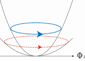
Figure 1: The schema of the effective potential of $\Phi_{1}$. Before $\Phi_{2}$ decays, $\Phi_{1}$ inside the $Q$-ball moves in a circular orbit shown as the dotted line. After the decay of $\Phi_{2}$, the amplitude of $\Phi_{1}$ decreases but its angular velocity increases so that the charge of $\Phi_{1}$ remains constant. The modified orbit is represented as the solid circle.

We would like to make several remarks. First, the $Q$-ball solution such as Eq. (III) exists if and only if the $Q$-ball solution is allowed before the decay of $\Phi_{2}$, that is to say, $K<0$. In other words, the partial decay of the constituent fields does not split the $Q$-ball into fragments. This is rather surprising result. For instance, even if $K_{1}$ is positive, the $Q$-ball configuration remains stable as long as $K$ is negative. It is the conservation of the charge of $\Phi_{1}$ that keeps the $Q$-ball stable during the course of the decay. After the decay of $\Phi_{2}$ completed, $\Phi_{1}$ still feels the potential of $\Phi_{2}$ through the $D$-term potential. Therefore $\Phi_{1}$ moves in an effective potential given as the sum of the potentials of $\Phi_{1}$ and $\Phi_{2}$. See Fig. 1. Second, the energy per unit charge becomes about $\sqrt{2}$ times larger, which means the $Q$-ball configuration becomes slightly unstable. The resultant $Q$-ball might be able to decay into light particles by using this increase. Such increment comes from the fact that the interplay of the charge conservation of $\Phi_{1}$ and the $D$-flat condition do not allow $\Phi_{2}$ to decay with the potential energy. Third, the reason why the energy of $\Phi_{1}$ cannot dissipate through the decay channel of $\Phi_{2}$ is that the $Q$-ball is a state of the lowest energy. It is helpful to consider how the $I$-ball Kasuya:2002zs , which is considered to be in an excited state of the $Q$-ball, change its profile if the partial decay occurs. The $I$-ball solution exists if the scalar potential is dominated by the quadratic term, which guarantees the approximate invariance of the adiabatic charge, $I$. The $I$-ball configuration is obtained as a state with the lowest energy at fixed $I$. Its profile is very similar to that of the $Q$-ball, except that the scalar field moves in an orbit with large ellipticity. If the kick of A-term is not strong enough, $I$-balls are generally formed instead of $Q$-balls. Let us consider the $I$-ball composed of $X=\Phi_{1}\Phi_{2}$, and suppose that $\Phi_{2}$ decays into something else. In this case, the energy of $\Phi_{1}$, in addition to $\Phi_{2}$, can dissipate into light particles through the $D$-term interaction. This process lasts until the ellipticity of the orbit becomes $\sim 1$, i.e., until the $I$-ball becomes a $Q$-ball, from which the energy cannot be extracted anymore without violating the charge conservation of $\Phi_{1}$.

IV Numerical Calculation

We have performed the numerical calculation to validate the analysis presented in the previous section. In particular, it is important to follow the evolution and show that the $Q$-ball does not break up during the decay of $\Phi_{2}$.

We have solved the equations of motion, Eq. (III), on the one dimensional lattices with the initial condition given as Eq. (21). The space $x$ and time $t$ are normalized by a mass scale $m$, while the field value is normalized by $M_{*}$. We take the following values for the model parameters: $m_{1}=m_{2}=m$, $\phi(0)/M_{*}=2$, $g^{2}M_{*}^{2}=200m^{2}$, $K_{1}=0.02$, $K_{2}=-0.1$, and $\Gamma=0.1m$.

The evolutions of $|\Phi_{1}|$ and $|\Phi_{2}|$ are illustrated in Fig. 2. As seen in the figure, the $D$-flat condition is satisfied inside the $Q$-ball but not outside. However, as shown in Figs. 3 and 4, the leakage of the energy or charge of $\Phi_{1}$ from the $Q$-ball is negligible . The amplitude decreases as expected by the analytical estimate (see Eq. (III)). The charge and energy of $\Phi_{1}$, $Q_{1}$ and $E_{1}$, do not change before and after the decay. See Figs. 3 and 4. On the other hand, the charge of $\Phi_{2}$ quickly decreases to zero, and its energy, $E_{2}$, is also brought down to the potential energy of $\Phi_{2}$, which is necessary to satisfy the $D$-flat condition. It should be noted that the shape of the $Q$-ball remains unchanged throughout the decay as expected. The behavior of the energy per unit charge, $E/Q$, is shown in Fig. 5, and it agrees well with the predicted values given in Eqs. (II.2) and (III).

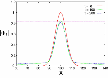
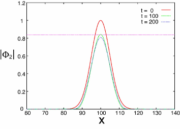
Figure 2: The evolution of the distribution of $|\Phi_{1}|$ and $|\Phi_{2}|$. The horizontal straight line represents the analytical estimate of $\tilde{\phi}$ given in Eq. (III). The $D$-flat condition is satisfied inside the $Q$-ball centered at $x=100$. The span of the lattices is actually $x=0\sim 200$.

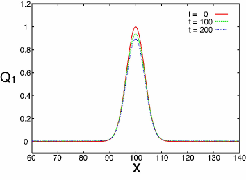
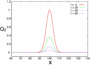
Figure 3: The evolution of the charge distribution of $\Phi_{1}$ and $\Phi_{2}$. While $Q_{1}$ is conserved, $Q_{2}$ rapidly decreases to zero due to the decay of $\Phi_{2}$. The charge outside the $Q$-ball is negligibly small.

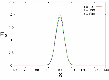
Figure 4: The evolution of the energy distribution. While $E_{1}$ stays unchanged, $E_{2}$ decreases to some finite value, which corresponds to the potential energy of $\Phi_{2}$. We do not have included the $D$-term potential in the definition of $E_{1,2}$.

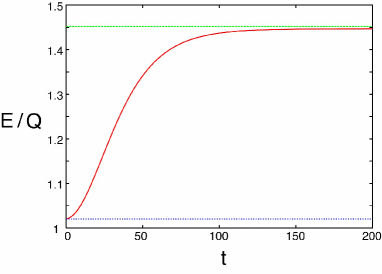
Figure 5: The time evolution of the energy per unit charge, $E/Q$. The analytical estimates for the initial and final states are shown as the horizontal straight lines.

V discussions

So far we have presented the analytical and numerical study of the partially decaying $Q$-balls with use of a toy model of flat directions. Let us consider now the implication of the results presented above. We have assumed that only a part of constituent fields decay, but our arguments apply to more generic case where there is a hierarchy between the decay rates, say, $\Gamma_{1}\gg\Gamma_{2}$. The asymmetry of the $Q$-ball continuously changes during the course of the decay. Most of the flat directions in the MSSM are composed of both squarks and sleptons, therefore they have both baryon and lepton number. If such a flat direction deforms into $Q$-balls and they are stable, our argument can be applied since the slepton condensate can always decay into a pair of neutrinos through the exchange of the gauginos. All through the decay processes, the $Q$-balls sequentially transform themselves toward pure $B$-balls with no lepton number. In the usual scenario considered so far, it is a flat direction composed only of squarks that forms pure $B$-balls. Therefore our analysis indicates that the pure $B$-balls are generated for most of flat directions, as a result of the decay into neutrinos. Specifically, all the $Q$-ball dark matter must be pure $B$-balls. Interestingly enough, the resultant $B$-ball might become unstable due to the increase of its energy per unit charge, leading to a complete decay of the $Q$-ball. In connection with the transformation of $Q$-balls into $B$-balls, the leptogenesis might become possible even for a flat direction with $B-L=0$. Another interesting possibility is that the $I$-ball can be naturally altered to Q-ball, if one of the constituent fields decay into something else. In particular, the $I$-ball composed of a flat direction that includes a leptonic field is generally transformed into a $Q$-ball. In fact, since the $I$-ball is a quasi-stable object, its conversion to a $Q$-ball was not known. The results of this study affords some new perspectives on the decay or stabilization processes of non-topological solitons made of flat directions.

In summary, we have investigated the evolution of $Q$-balls, assuming that some of the constituent scalar fields decay into light particles. With a toy model of the flat direction, we have obtained the analytical solution of the $Q$-ball in the final state, and found that the spatial shape of the $Q$-ball does not change, but the orbit of the scalar field inside the $Q$-ball does change in order to compensate for the decay. In particular, the energy per unit charge generally increases due to the partial decay, which might induce further decay of the remnant scalar fields. Also we have performed numerical calculations to confirm these results. Again we stress that $Q$-balls remain $Q$-balls throughout the partial decay, due to both the charge conservation of the remnant scalar fields and the $D$-flat condition.

ACKNOWLEDGMENTS

This work was partially supported by the JSPS Grant-in-Aid for Scientific Research No. 10975 (F.T.)

References

- (1) S. R. Coleman, Nucl. Phys. B 262, 263 (1985) [Erratum-ibid. B 269, 744 (1986)].
- (2) S. Kasuya, M. Kawasaki and F. Takahashi, Phys. Lett. B 559, 99 (2003) [arXiv:hep-ph/0209358].
- (3) I. Affleck and M. Dine, Nucl. Phys. B 249, 361 (1985); M. Dine, L. Randall and S. Thomas, Nucl. Phys. B 458, 291 (1996) [arXiv:hep-ph/9507453].
- (4) A. Kusenko and M. E. Shaposhnikov, Phys. Lett. B 418, 46 (1998) [arXiv:hep-ph/9709492].
- (5) K. Enqvist and J. McDonald, Nucl. Phys. B 538, 321 (1999) [arXiv:hep-ph/9803380].
- (6) S. Kasuya and M. Kawasaki, Phys. Rev. D 61, 041301 (2000) [arXiv:hep-ph/9909509].
- (7) S. Kasuya and M. Kawasaki, Phys. Rev. D 62, 023512 (2000) [arXiv:hep-ph/0002285].
- (8) S. Kasuya and M. Kawasaki, Phys. Rev. Lett. 85, 2677 (2000) [arXiv:hep-ph/0006128].
- (9) S. Kasuya and M. Kawasaki, Phys. Rev. D 64, 123515 (2001) [arXiv:hep-ph/0106119].
- (10) M. Kawasaki, F. Takahashi and M. Yamaguchi, Phys. Rev. D 66, 043516 (2002) [arXiv:hep-ph/0205101].
- (11) K. Ichikawa, M. Kawasaki and F. Takahashi, arXiv:astro-ph/0402522.
- (12) F. Takahashi and M. Yamaguchi, arXiv:hep-ph/0308173, (to be published in Phys. Rev. D).
- (13) A. G. Cohen, S. R. Coleman, H. Georgi and A. Manohar, Nucl. Phys. B 272, 301 (1986).