HD-THEP-04-09

hep-ph/0403197

The Perturbative Odderon in Quasidiffractive

Photon-Photon Scattering

Stefan Braunewell ^a, Carlo Ewerz ^b

Institut für Theoretische Physik, Universität Heidelberg
Philosophenweg 16, D-69120 Heidelberg, Germany

We study the perturbative Odderon in the quasidiffractive process $\gamma^{(*)}\gamma^{(*)}\to\eta_{c}\eta_{c}$. At high energies this process is dominated by Odderon exchange and can be viewed as the theoretically cleanest test of the perturbative Odderon. We calculate the differential and total cross section, as well as the dependence on the energy and on the photon virtualities taking into account the effects of resummation of logarithms of the energy. The results are compared with those obtained with a simple exchange of three noninteracting gluons. We present the expected cross section for this process at a future Linear Collider and discuss implications for other processes involving the perturbative Odderon.

  ^a email: S.Braunewell@thphys.uni-heidelberg.de
^b email: C.Ewerz@thphys.uni-heidelberg.de

1 Introduction

The Odderon is the partner of the Pomeron carrying negative charge parity quantum number. In high energy scattering processes it gives the leading contribution to processes in which negative $C$-parity is exchanged in the $t$-channel.

After the concept of the Odderon had been proposed in [1], it was for a long time almost exclusively discussed in the context of elastic or inclusive processes. These have the disadvantage that the Odderon gives only one of many contributions to the scattering amplitude and a clean identification of the Odderon is rather difficult. The only experimental evidence of the Odderon so far has been found as a small difference between the differential cross sections of elastic proton-proton and antiproton-proton scattering at the CERN ISR [2]. Due to the low statistics of the data and the difficulty of extracting the Odderon contribution, however, it is not possible to interpret this as an unambiguous signal of the Odderon. For a more detailed review of the phenomenological and theoretical status of the Odderon we refer the reader to [3].

Recently an important change of direction in the search for the Odderon has taken place. Now the search concentrates on processes in which it basically gives the only contribution to the cross section. The cross section for such processes is in general smaller than for elastic or inclusive processes, but here already the observation of the process as such would establish the existence of the Odderon. Examples of such exclusive processes are the double-diffractive production of vector mesons in proton-(anti)proton scattering [4] or the diffractive production of pseudoscalar or tensor mesons in electron-proton scattering [5]-[15]. In all of these processes Odderon exchange gives the main contribution to the cross section at high energies. Other possible contributions can only arise due to photon or reggeon exchange, but both of these contributions are under good theoretical control. Another interesting possibility is to study the interference between Pomeron and Odderon exchange. This is possible in the diffractive production of final states that can be produced both in a $C=+1$ and in a $C=-1$ state like for example a pair of charged pions. The interference term between the two corresponding production mechanisms can be isolated in suitable asymmetries like for example the charge or spin asymmetry. Asymmetries of this kind have been studied in [16]-[20]. Also here already the experimental observation of an asymmetry could firmly establish the existence of the Odderon.

The first experimental search for one of these exclusive processes was performed for the case of diffractive pion photoproduction in $ep$ scattering at HERA in [21]. This process is the one for which the largest cross section is expected, but its theoretical description obviously has to rely on nonperturbative techniques. Such a calculation was performed in [11] making use of the stochastic vacuum model [22, 23, 24] in the framework of the functional approach to high energy scattering developed in [25]. In [21] the experimental results have been compared to the expectations based on that calculation, and no signal of Odderon exchange has been found. The failure of the theoretical prediction for this process is currently not understood.

In order to avoid the large theoretical uncertainties of nonperturbative calculations in diffractive pion production one can consider the diffractive production of heavy pseudoscalar or tensor mesons. In that case the large mass of the meson provides a hard scale, and one can hope that perturbation theory is applicable even for real photons. Here in particular the production of $\eta_{c}$ mesons has been considered, see [7, 8, 13]. The expected cross section for that process was in the range of several tens of picobarns. In a study of elastic $pp$ scattering it has subsequently been found that the choice of parameters in the Odderon-proton coupling in those calculations was very optimistic [26], and a realistic estimate of the cross section should be even smaller by at least an order of magnitude. Due to the small cross section, the process is not of immediate phenomenological interest, but it has turned out to be quite interesting from a theoretical perspective.

That interest is related to the occurrence of large logarithms of the energy in the perturbative series. In the simplest possible perturbative picture the exchange of an Odderon is described by the exchange of three noninteracting gluons in a symmetric color state. In higher orders in perturbation theory large logarithms of the energy can compensate the smallness of the strong coupling constant, $\alpha_{s}\log s\sim 1$, and one needs to resum these logarithms. For the case of the Odderon this leads to the generalized leading logarithmic approximation (GLLA) which is encoded in the Bartels-Kwieciński-Praszałowicz (BKP) equation. Recently two different solutions of this equation have been found explicitly in [29] and in [30]. The former solution does not couple to the $\gamma\eta_{c}$ impact factor in leading order and is hence not relevant for the production of $\eta_{c}$ mesons. The latter solution, the so-called Bartels-Lipatov-Vacca (BLV) solution, on the other hand does couple to that impact factor. Its intercept exactly equals one, and it hence leads to a cross section which is constant with the energy up to logarithmic corrections. The BLV solution was recently also found in the dipole picture of high energy scattering [31].

Although the intercept of the BLV solution is equal to the intercept of the simple three-gluon exchange model for the Odderon it has quite different properties. So far the phenomenological consequences of using the BLV solution in the scattering amplitude have been considered only in the diffractive production of $\eta_{c}$ mesons in [13, 14]. Interestingly, in [13] it was found that for real photons the resulting cross section is by about a factor of five larger than the one obtained in [7, 8] by using a simple three-gluon exchange for describing the Odderon. It is a very interesting question whether that enhancement is a general property of the BLV solution or whether and how strongly it depends on the couplings of the Odderon to the proton and to the $\gamma\eta_{c}$ impact factor. It is one of the aims of the present paper to address this question.

All of the processes mentioned above involve the coupling of the Odderon to the proton. This coupling is known to be rather sensitive to the internal structure of the proton [26], and it is therefore possible that due to nonperturbative effects this coupling is small. In that case it could be quite difficult to find the Odderon in these processes. It is therefore interesting to study also processes which do not involve the uncertainties of the Odderon-proton coupling. From a theoretical point of view the quasidiffractive process $\gamma^{(*)}\gamma^{(*)}\to\eta_{c}\eta_{c}$ is the cleanest possible probe of the Odderon. Due to the large mass of the charm quark the coupling of the Odderon to the $\gamma\eta_{c}$ impact factor can be calculated perturbatively even for small photon virtualities. Again, already the observation of this process at high energies would firmly establish the existence of the Odderon. More generally, one can study the quasidiffractive processes $\gamma^{(*)}\gamma^{(*)}\to MM$ and $\gamma^{(*)}\gamma^{(*)}\to MX$ with $M$ being a heavy pseudoscalar or tensor meson. Also these can occur at high energies only due to Odderon exchange. Such processes have first been studied in [32, 33] and more recently for the case of $\eta_{c}$ meson production in [34]. In these studies the Odderon has been modeled as a simple exchange of three noninteracting gluons.

In the present paper we study in detail the process $\gamma^{(*)}\gamma^{(*)}\to\eta_{c}\eta_{c}$ at high energies. In particular, we take into account the effects of resumming large logarithms of the energy in perturbation theory by using the BLV solution of the BKP equation. That allows us to perform a detailed study of the properties of the BLV Odderon solution in a completely perturbative process, that is in a clean theoretical setting which does not involve model assumptions about the impact factors. The properties of the BLV Odderon can easily be compared to those of an Odderon modeled by the exchange of three noninteracting gluons. Furthermore, by comparing the behavior of the BLV solution in this process and in the process $\gamma p\to\eta_{c}p$ we can draw some conclusions about the possible origin of the enhancement obtained in the latter process for the BLV solution as compared to simple three-gluon exchange. Another important motivation for the present study is to estimate the chances of finding the Odderon in the process $\gamma^{(*)}\gamma^{(*)}\to\eta_{c}\eta_{c}$ in $e^{+}e^{-}$ scattering at a future Linear Collider.

In section 2 we provide the cross section formulae for the process $\gamma^{(*)}\gamma^{(*)}\to\eta_{c}\eta_{c}$. In particular we discuss the BLV solution and the $\gamma\eta_{c}$ impact factor. In section 3 we study the resulting cross section and its dependence on the different parameters. After discussing some technical details of the calculation, we start with the case of real photons and calculate the differential and total cross sections in section 3.2. The applicability of the saddle point approximation for the BLV Odderon solution in this process is considered in 3.3. We investigate the energy dependence of the cross section in section 3.4. In section 3.5 we address the possibility to observe this process at a future Linear Collider. The case of virtual photons is studied in section 3.6. Finally, we discuss our results in the light of results obtained for the BLV solution in the process $\gamma p\to\eta_{c}p$ in section 3.7. Our main results are summarized in section 4.

2 The scattering amplitude

2.1 High energy factorization

We consider the process $\gamma^{(*)}\gamma^{(*)}\to\eta_{c}\eta_{c}$ at high energy and relatively small momentum transfer, that is $s\gg|t|$ in terms of Mandelstam variables. The photons in the initial state can both be real or virtual. The large mass of the charm quark provides a justification for treating the process in perturbation theory.

At high energies the process is dominated by Odderon exchange. Diagrams involving quark exchange in the $t$-channel are suppressed by powers of the energy and can be neglected at the energies which we will consider below. Due to high energy factorization the scattering amplitude for Odderon exchange can be written in the form illustrated in figure 1.

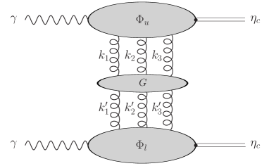
Figure 1: Factorized form of the scattering amplitude for $\gamma^{(*)}\gamma^{(*)}\to\eta_{c}\eta_{c}$

The amplitude is a convolution of the Odderon Green function $\mathbf{G}$ with two impact factors $\Phi$ coupling the Odderon to the external particles. Symbolically,

$${\cal A}\sim\langle\Phi_{u}|\mathbf{G}|\Phi_{l}\rangle\,,$$ (1)

and the convolution includes the integration over the unconstrained transverse momenta of the gluons as will be described further below. The subscripts $u$ and $l$ of the impact factors stand for the upper and lower impact factor, respectively. For the Odderon Green function $\mathbf{G}$ one can insert either the BLV Odderon solution or the propagation of three noninteracting gluons as the simplest possible model for the perturbative Odderon.

In order to make the paper self-contained we collect in the following sections the known results for the impact factors and for the Odderon Green function, and we bring them into a form which can then be used to compute the above amplitude and the resulting cross section.

2.2 The $\gamma\to\eta_{c}$ impact factor

We first consider the impact factor that describes the transition of a photon (real or virtual) into an $\eta_{c}$ meson and three $t$-channel gluons in a color singlet state as it has been calculated in [7]. There it was found that the impact factor has only transverse components. The resulting expression reads

$$\Phi^{i}=b\epsilon^{i}_{l}\left(\sum_{(123)}\frac{(\mathbf{k}_{1}+\mathbf{k}_{2}-\mathbf{k}_{3})^{l}}{Q^{2}+4m_{c}^{2}+(\mathbf{k}_{1}+\mathbf{k}_{2}-\mathbf{k}_{3})^{2}}-\frac{\mathbf{q}^{l}}{Q^{2}+4m_{c}^{2}+\mathbf{q}^{2}}\right),\qquad i=1,2\,,$$ (2)

where the sum runs over all cyclic permutations and the index $i$ corresponds to the two possible transverse polarizations of the incident photon. Furthermore, $\mathbf{q=k}_{1}+\mathbf{k}_{2}+\mathbf{k}_{3}$ is the total momentum transfer, and we will have $t=-\mathbf{q}^{2}$. $Q^{2}$ is the virtuality of the photon, $m_{c}=1.4\,\mbox{GeV}$ the mass of the charm quark, $\epsilon_{l}^{i}$ the totally antisymmetric tensor in two dimensions, and we have

$$b=\frac{4}{q_{c}}\frac{d^{abc}}{N_{c}}\sqrt{\frac{\alpha_{s}^{3}}{\alpha}\pi^{3}\Gamma m_{\eta_{c}}}\,.$$ (3)

Here $\alpha_{s}$ and $\alpha$ are the strong and electromagnetic coupling constants, respectively. The charm quark carries the charge $q_{c}=2/3$, and the $\eta_{c}$ meson has a radiative (photon) width of $\Gamma=7\,\mbox{keV}$ and a mass of $m_{\eta_{c}}=2.98\,\mbox{GeV}$.

The factor $d^{abc}$ is the totally symmetric structure constant for the color SU($N_{c}$) group. The scattering amplitude contains the contraction

$$d^{abc}d^{abc}=\frac{N_{c}^{2}-4}{N_{c}}\,\delta^{aa}=\frac{40}{3}\,,$$ (4)

where the last equality holds for $N_{c}=3$.

2.3 The BLV solution

The Bartels-Lipatov-Vacca (BLV) Odderon solution $\Psi^{(\nu,n)}$ found in [30] is constructed from the known eigenfunctions $E^{(\nu,n)}$ of the BFKL equation [35, 36]. These eigenfunctions are labeled by a discrete quantum number $n\in{\rm\kern 2.59995pt\vrule width=0.20004pt,height=2.15277pt,depth=0.0pt\kern 0.39993pt\vrule width=0.20004pt,height=6.32915pt,depth=-4.30554pt\kern-3.39996ptZ}$, called the conformal spin, and a continuous quantum number $\nu\in{\rm I\kern-2.10007ptR}$. The functions $E^{(\nu,n)}$ were found in impact parameter space in [37], and they can be obtained in transverse momentum space via a Fourier transformation. We will use the same symbol $E^{(\nu,n)}$ for both representations of the BFKL eigenfunctions. In the BLV solution the eigenfunctions of the BKP integral operator are constructed as

$$\Psi^{(\nu,n)}(\mathbf{k}_{1},\mathbf{k}_{2},\mathbf{k}_{3})=c(\nu,n)\sum_{(123)}\frac{(\mathbf{k}_{1}+\mathbf{k}_{2})^{2}}{\mathbf{k}_{1}^{2}\mathbf{k}_{2}^{2}}E^{(\nu,n)}(\mathbf{k}_{1}+\mathbf{k}_{2},\mathbf{k}_{3})\,,$$ (5)

where the sum runs over cyclic permutations, and $n$ needs to be an odd integer. We use the same normalization convention as in [13], so that the Odderon states have the same norm as the Pomeron eigenfunctions of which they are constructed. This leads to

$$c(\nu,n)=\sqrt{\frac{N_{c}\alpha_{s}}{2\pi^{2}(-3\chi(\nu,n))}}\,.$$ (6)

The functions (5) are eigenfunctions of the BKP integral operator with eigenvalues

$$\chi(\nu,n)=\frac{N_{c}\alpha_{s}}{\pi}\left[2\psi(1)-\psi\left(\frac{1+|n|}{2}+i\nu\right)-\psi\left(\frac{1+|n|}{2}-i\nu\right)\right]\,,$$ (7)

where $\psi$ is the logarithmic derivative of the Euler gamma function $\Gamma$.

The Odderon Green function in spectral representation is constructed as a superposition of all states with odd integer numbers $n$ and general (real) $\nu$,

$$\mathbf{G}=\sum_{\mathrm{odd\ n\ }}\int_{-\infty}^{\infty}d\nu\,e^{y\chi(\nu,n)}\frac{(2\pi)^{2}(\nu^{2}+\frac{n^{2}}{4})}{[\nu^{2}+\frac{(n-1)^{2}}{4}][\nu^{2}+\frac{(n+1)^{2}}{4}]}\Psi^{(\nu,n)}(\mathbf{k}_{1},\mathbf{k}_{2},\mathbf{k}_{3}){\Psi^{*(\nu,n)}}(\mathbf{k}_{1}^{\prime},\mathbf{k}_{2}^{\prime},\mathbf{k}_{3}^{\prime})\,.$$ (8)

Here $y=\log(s/s_{0})$ is the rapidity and $s_{0}$ is a fixed energy scale. The scale $s_{0}$ is undetermined in leading logarithmic approximation, and we will discuss possible choices for $s_{0}$ in section 3.4 below. The normalization in (8) is chosen in such a way that in the limit of vanishing coupling, $\alpha_{s}\to 0$, the Green function reduces to the exchange of three noninteracting gluons.

In order to calculate the momentum integral for the scattering amplitude, we need to know the BFKL eigenfunctions in momentum space. In impact parameter space the eigenfunctions are

$$E^{(\nu,n)}(\mathbf{r}_{10},\mathbf{r}_{20})=\left(\frac{r_{12}}{r_{10}r_{20}}\right)^{h}\left(\frac{\bar{r}_{12}}{\bar{r}_{10}\bar{r}_{20}}\right)^{\bar{h}}\,,$$ (9)

where $\mathbf{r}_{ij}=\mathbf{r}_{i}-\mathbf{r}_{j}$. In the r.h.s. we use complex coordinates $r_{i}$ for describing positions in the two-dimensional impact parameter space. Further we have the conformal weights $h=(1+n)/2+i\nu$ and $\bar{h}=1-h^{*}=(1-n)/2+i\nu$.

The Fourier transform of these eigenfunctions was calculated in [13]. It was found that the momentum space functions have the form

$$E^{(\nu,n)}(\mathbf{l}_{1},\mathbf{l}_{2})=E_{A}^{(\nu,n)}(\mathbf{l}_{1},\mathbf{l}_{2})+E_{\delta}^{(\nu,n)}(\mathbf{l}_{1},\mathbf{l}_{2})\,,$$ (10)

where $E_{A}^{(\nu,n)}$ denotes an analytic contribution and $E_{\delta}^{(\nu,n)}$ a part containing $\delta$-functions. The analytic part reads

$$E_{A}^{(\nu,n)}(\mathbf{l}_{1},\mathbf{l}_{2})=C[X(\mathbf{l}_{1},\mathbf{l}_{2})-X(\mathbf{l}_{2},\mathbf{l}_{1})]\,,$$ (11)

where the coefficient $C$ is

$$C=\frac{(-i)^{n}}{(4\pi)^{2}}h\bar{h}(1-h)(1-\bar{h})\Gamma(1-h)\Gamma(1-\bar{h})\,.$$ (12)

The expression $X$ can be given in terms of the hypergeometric function $F(a_{1},a_{2};b;z)={}_{2}F_{1}(a_{1},a_{2};b;z)$,

$$X(\mathbf{l}_{1},\mathbf{l}_{2})=\left(\frac{l_{1}}{2}\right)^{\bar{h}-2}\left(\frac{\bar{l}_{2}}{2}\right)^{h-2}F\left(1-h,2-h;2;-\frac{\bar{l}_{1}}{\bar{l}_{2}}\right)F\left(1-\bar{h},2-\bar{h};2;-\frac{l_{2}}{l_{1}}\right)\,.$$ (13)

The two-dimensional momenta are denoted as complex numbers on the r.h.s.

The $\delta$-function part in (10) is simpler. Denoting the total momentum transfer (in complex notation) by $q=l_{1}+l_{2}$, it can be written as

$$E_{\delta}^{(\nu,n)}(\mathbf{l}_{1},\mathbf{l}_{2})=\left[\delta^{(2)}(\mathbf{l}_{1})+(-1)^{n}\delta^{(2)}(\mathbf{l}_{2})\right]\frac{i^{n}}{2\pi}2^{1-h-\bar{h}}\frac{\Gamma(1-\bar{h})}{\Gamma(h)}q^{\bar{h}-1}q^{*h-1}\,.$$ (14)

2.4 Calculation of the scattering amplitude

We want to calculate the scattering amplitudes

$$A^{ij}=\frac{s}{3(2\pi)^{4}}\langle\Phi^{i}_{u}|\mathbf{G}|\Phi^{j}_{l}\rangle$$ (15)

for different transverse polarizations $i,j$ of the incoming photons, where we have distributed the constant factors as in [8]. In order to compute these expressions, we have to evaluate integrals over the independent transverse momenta, e.g.

$$\langle\Phi^{i}|\Psi^{(\nu,n)}\rangle=\int d^{2}\mathbf{k}_{1}d^{2}\mathbf{k}_{2}\,\Phi^{i}(\mathbf{k}_{1},\mathbf{k}_{2};\mathbf{q})\Psi^{(\nu,n)}(\mathbf{k}_{1},\mathbf{k}_{2};\mathbf{q})\,.$$ (16)

However, this four-dimensional integral reduces to a two-dimensional one [30],

$$\langle\Phi^{i}|\Psi^{(\nu,n)}\rangle=\frac{b}{c(\nu,n)}\int d^{2}{\bf k}\,\phi^{i}(\mathbf{k,q-k})E^{(\nu,n)}\mathbf{(k,q-k)}\equiv\frac{b}{c(\nu,n)}\langle\phi^{i}|E^{(\nu,n)}\rangle\,,$$ (17)

where the reduced impact factor is

$$\phi^{i}(\mathbf{k,q-k})=\frac{\epsilon^{i}_{l}(2\mathbf{k}-\mathbf{q})^{l}}{Q^{2}+4m_{c}^{2}+(2\mathbf{k}-\mathbf{q})^{2}}\,.$$ (18)

Let us now consider the infinite sum over odd values of $n$ in (8) which needs approximation in order to be evaluated numerically. In the full Green function (8) the exponential factor $e^{y\chi(\nu,n)}$ clearly is of special importance to the integrand, and an expansion of its argument can help us determine the dominant values of $n$. Expanding (7) up to second order around $\nu=0$ yields

$$\chi(\nu,n)=\frac{N_{c}\alpha_{s}}{\pi}\left[2\,\psi(1)-2\psi\left(\frac{1+|n|}{2}\right)+\psi^{\prime\prime}\left(\frac{1+|n|}{2}\right)\,\nu^{2}+\mathcal{O}(\nu^{4})\right]\,.$$ (19)

For values of $n$ other than $\pm 1$ we therefore get a constant part in the Taylor expansion of the argument of the exponential which grows with $n$. We have in fact checked numerically the contribution of $n=3$ and find that this term is already of relative size $\sim 10^{-4}$ compared to the leading term. Therefore we can reduce the sum to one over $n=\pm 1$.

Now we can further simplify the integral that we have to calculate numerically. The analytic part reduces for $n=\pm 1$ to

$$E^{(\nu,n=\pm 1)}_{A}(\mathbf{k,q-k})=\pm\frac{1}{(4\pi)^{2}}\nu(1+\nu^{2})\Gamma^{2}(1-i\nu)[X(\mathbf{k,q-k})-X(\mathbf{q-k,k})]\,.$$ (20)

For $n=1$, (13) leads to

$$X^{(n=1)}(\mathbf{k,q-k}) = \left(\frac{k}{2}\right)^{i\nu-2}\left(\frac{\bar{q}-\bar{k}}{2}\right)^{i\nu-1}F\left(-i\nu,1-i\nu;2;-\frac{\bar{k}}{\bar{q}-\bar{k}}\right)$$ (21)

$${}\times\,F\left(1-i\nu,2-i\nu;2;-\frac{q-k}{k}\right)\,.$$

For $n=-1$, we get

$$X^{(n=-1)}(k,q-k)=X^{(n=1)}(\bar{q}-\bar{k},\bar{k})\,,$$ (22)

and thus obtain

$$E_{A}^{(\nu,n=-1)}(k,q-k)=E_{A}^{(\nu,n=1)}(\bar{k},\bar{q}-\bar{k})\,.$$ (23)

From now on we choose the coordinate axes such that the total momentum transfer $\mathbf{q}$ is in 1-direction, so that in complex notation $q$ is purely real. As we have an integral over both components of the two-dimensional momentum vector $\mathbf{k}$, we can replace the second component by its negative value, which in complex notation corresponds to complex conjugation. In the reduced impact factor (18) we have to switch the sign of the $i=1$ component due to the $\epsilon$ symbol. The $i=2$ expression remains unchanged because it includes only the first component of the momentum in its numerator. For $i\neq j$ in (15) the coherent sum over $n=\pm 1$ thus gives two equal but opposite results. For parallel photon polarizations, $i=j$, the resulting expression in (15) is the same for $n=1$ and $n=-1$. Thus, we can work with the expression $E_{A}^{(\nu,n=1)}$, which we will denote as $E_{A}^{(\nu)}$ from now on.

Let us now turn to the $\delta$-function part for $n=\pm 1$. For the $\delta$-function part one also obtains the same result for $n=+1$ and $n=-1$, which we will denote by $E^{(\nu)}_{\delta}$,

$$E^{(\nu)}_{\delta}=E^{(\nu,n=\pm 1)}_{\delta}(\mathbf{k,q-k})=\left[\delta^{(2)}(\mathbf{k})-\delta^{(2)}(\mathbf{q-k})\right]\frac{i}{2\pi}4^{-i\nu}\frac{\Gamma(1-i\nu)}{\Gamma(1+i\nu)}\frac{q^{2i\nu}}{q}\,.$$ (24)

With our specific choice $\mathbf{q}=(q,0)$ we can easily evaluate the convolution of the $\delta$-function part with the impact factor. We can see from (18) that due to the $\epsilon$ tensor the $i=1$ component of the impact factor vanishes for $\mathbf{k}=0$ or $\mathbf{k=q}$, that is when the $\delta$-functions in (24) are applied. Hence the only non-vanishing contribution to the convolution of the $\delta$-function part with the impact factor is the one for $i,j=2$,

$$\langle\phi^{i=2}|E^{(\nu)}_{\delta}\rangle=\frac{i}{\pi}\frac{1}{4^{i\nu}}\frac{\Gamma(1-i\nu)}{\Gamma(1+i\nu)}\frac{q^{2i\nu}}{Q^{2}+4m_{c}^{2}+q^{2}}\,.$$ (25)

2.5 Saddle point approximation

In [13] diffractive production of an $\eta_{c}$ meson in $\gamma p$ scattering was calculated in the saddle point approximation (SPA). For our study this approximation will not be needed, and our results given below will not make use of the SPA. Nevertheless, it is interesting for us to study the same approximation also for our scattering process in order to discuss our results in the context of those of [13]. For this purpose the $\nu$ integral in (8) is approximated by expanding the argument of the exponential and other $\nu$-dependent factors in the integrand (in particular the BFKL eigenfunctions) in Taylor series. In lowest non-vanishing order the Lipatov characteristic function (7) is quadratic in $\nu$,

$$\chi(\nu,\pm 1)=-2\frac{N_{c}\alpha_{s}}{\pi}\zeta(3)\nu^{2}+\mathcal{O}(\nu^{4})\,.$$ (26)

The rest of the integrand is also expanded in $\nu$. The first non-vanishing term in the expansion of the analytic part is of first order, but this term vanishes in the momentum integral because it is orthogonal to the $\eta_{c}$ impact factor, see [13]. The first term that survives this convolution is of second order. The $\delta$-function part leads to a non-vanishing contribution already in zeroth order in $\nu$,

$$E^{(\nu)}_{\delta,0}(\mathbf{k}_{1},\mathbf{k}_{2})=\left(\delta^{(2)}(\mathbf{k}_{1})-\delta^{(2)}(\mathbf{k}_{2})\right)\frac{i}{2\pi}\frac{1}{q}\,.$$ (27)

Therefore in [13] only the $\delta$-contribution is calculated. We will study in section 3.3 below how that approximation affects our results. As we will show, the SPA turns out to be inadequate for our process.

3 Numerical results

3.1 Details of the calculation

In the following sections we will present our numerical results for the cross section for $\gamma^{(*)}\gamma^{(*)}\to\eta_{c}\eta_{c}$ and for its dependence on various parameters. In the present section we make several general remarks relevant for those results.

The differential cross section is obtained from the amplitudes $A^{ij}$ involving the BLV Odderon solution as

$$\frac{d\sigma}{dt}=\frac{1}{16\pi s^{2}}\frac{1}{4}\sum_{i,j=1}^{2}|A^{ij}|^{2}\,.$$ (28)

As we have seen in the previous section, the mixed polarization amplitudes vanish. Furthermore, we find numerically that the $i,j=1$ contribution to the cross section is only $\sim 1\%$ of that coming from $i,j=2$. Since the numerical error of our calculation is also on the percent level we neglect this contribution. We hence have

$$\frac{d\sigma}{dt}=\frac{1}{64\pi s^{2}}|A|^{2},$$ (29)

where $A=A^{22}$. According to the discussion above we obtain the scattering amplitude $A$ as the integral

$$A=2\frac{s}{3(2\pi)^{4}}\int_{-\infty}^{\infty}d\nu\,e^{y\chi(\nu)}\frac{(2\pi)^{2}(\nu^{2}+\frac{1}{4})}{\nu^{2}(\nu^{2}+1)}\frac{b^{2}}{c(\nu)^{2}}\langle\phi|E^{(\nu)}\rangle_{u}\langle\phi|E^{(\nu)}\rangle^{*}_{l}\,,$$ (30)

where we have the reduced impact factor $\phi=\phi^{i=2}$, and the convolution of $\phi$ with $E^{(\nu)}$ is defined in (17). Further, $E^{(\nu)}$ has two parts as in (10), and we have set $n=+1$ here while multiplying by 2 to take into account the contribution of $n=-1$ as explained in the previous section.

Our results below are obtained from a numerical evaluation of the integral (30). We emphasize that we compute that integral without further approximations. In particular we do not use the saddle point approximation for our main results. The outcome of using the SPA is included below only in order to discuss the applicability of that approximation. In fact we will show that the saddle point approximation is not applicable to our process in the phenomenologically relevant kinematical region.

Recall that the convolutions $\langle\phi|E^{(\nu)}\rangle_{u,l}$ in the integrand of (30) involve only two-dimensional integrations, see (17). The reduction from a four-dimensional to a two-dimensional integral in these convolutions occurred due to the special structure of the BLV Odderon solution. The integral (30) involves hypergeometric functions which are expensive to evaluate in terms of computer time. But because of the reduction to two-dimensional integrations in $\langle\phi|E^{(\nu)}\rangle_{u,l}$ it is still possible to perform the integral (30) using Mathematica.

As already pointed out in section 2.4, we do not take into account contributions to the BLV solution with quantum number $n\neq\pm 1$. We have in fact calculated numerically the $n=3$ contribution for a variety of values of the parameters $Q^{2}$, $s$ and $t$ and find it to be negligible.

One of the most interesting questions which we want to study is how the BLV Odderon solution compares to the exchange of three noninteracting gluons in our process. The latter exchange is the simplest possible perturbative model for the Odderon. Technically speaking it amounts to replacing the Odderon Green function $\mathbf{G}$ in (15) by three free gluon propagators,

$$\mathbf{G}_{3g}=\delta^{(2)}(\mathbf{k}^{\prime}_{1}-\mathbf{k}_{1})\delta^{(2)}(\mathbf{k}^{\prime}_{2}-\mathbf{k}_{2})\,\frac{1}{\mathbf{k}_{1}^{2}\mathbf{k}_{2}^{2}\mathbf{k}_{3}^{2}}\,.$$ (31)

The cross section for $\gamma^{(*)}\gamma^{(*)}\to\eta_{c}\eta_{c}$ with a simple three-gluon exchange was calculated in [34]. We have reproduced the results of that paper in order to compare them with our calculations.

Our calculation is based on the BLV Odderon solution which results from the resummation of leading logarithms. It should be pointed out that there are several uncertainties which are inevitable in that approximation scheme. The first of these uncertainties concerns the choice of the appropriate value of the strong coupling constant. Strictly speaking the scale of $\alpha_{s}$ is undetermined in GLLA. In all our calculations we use $\alpha_{s}=\alpha_{s}(m_{c}^{2})=0.38$ to allow for an easy comparison with the results from [34] and [13] where the same value had been chosen. It should be emphasized, however, that already a small change in $\alpha_{s}$ implies a considerable change in the cross section. This is due to the simple fact that the cross section contains a factor $\alpha_{s}^{6}$ already from the coupling of the three gluons to the impact factors.

Another important uncertainty is the choice of the energy scale $s_{0}$ in $y=\log(s/s_{0})$. Also this scale is, strictly speaking, undetermined in GLLA and has to be chosen as a typical energy scale for the process. We will discuss several possible choices in detail in section 3.4. It will turn out that choices which appear equally natural can lead to quite different results.

Of course there is a minimal momentum transfer required for the transition from a real photon in the initial state to a $\eta_{c}$ meson in the final state. That minimal momentum transfer $t_{\mathrm{min}}$ can be estimated to be $t_{\mathrm{min}}\approx-m_{\eta_{c}}^{4}/s$. At the energies which we will consider its numerical value will be very small and will not have any quantitative effect visible in our figures.

3.2 Cross section for the scattering of real photons

For the calculations in this section we choose a center-of-mass energy $\sqrt{s}=300$ GeV. This choice is somewhat arbitrary and our main motivation for it is that later on we want to compare the behavior of the BLV solution in the process $\gamma\gamma\to\eta_{c}\eta_{c}$ to that in the process $\gamma p\to\eta_{c}p$. The latter was calculated for the HERA energy in [13], and we therefore use the same energy here. As the process $\gamma\gamma\to\eta_{c}\eta_{c}$ is phenomenologically interesting mainly as a subprocess of electron-positron scattering for example, in an actual collider setup there is a continuous energy range available for the $\gamma\gamma$ scattering, rather than a fixed center-of-mass energy. We give an estimate on the size of the cross section for the process $e^{+}e^{-}\to\eta_{c}\eta_{c}$ in section 3.5, but in the first part we are only concerned with the properties of the differential cross section of the subprocess. The squared energy $s$ enters in the argument of the exponential as $y=\log(s/s_{0})$, with the scale factor $s_{0}$ on which we will comment later. For this section we use a scale $s_{0}=m_{\eta_{c}}^{2}$. Our numerical results for the differential cross section for real photons (virtuality $Q^{2}=Q_{u,l}^{2}=0$) are shown in figure 2, together with the corresponding results for the noninteracting three-gluon process from [34].

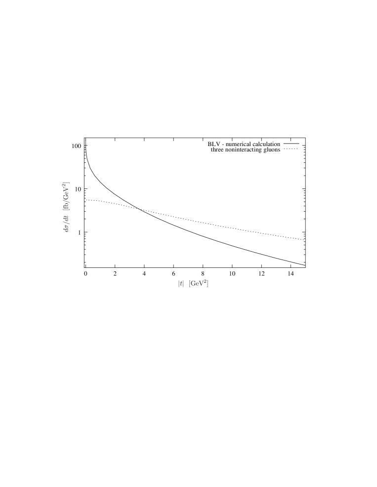
Figure 2: Results for the differential cross section $\frac{d\sigma}{dt}$ for real photons ($Q^{2}=0$) and center-of-mass energy $\sqrt{s}=300\,\mbox{GeV}$

Comparing our numerical results for the BLV solution to the three noninteracting gluons in the $t$-channel, we find a huge enhancement of the differential cross section at small momentum transfer. The cross section calculated with the BLV solution reaches a maximal value of $\approx 120$ fb/GeV² at $t=t_{\mathrm{min}}\approx-10^{-3}\,\mbox{GeV}^{2}$, and then quickly falls to $\approx 88$ fb/GeV² already at $|t|=0.01$ GeV². The simple solution exhibits a fundamentally different $t$-dependence that can fairly well be described by an exponential decay. Its maximal value at $t=t_{\mathrm{min}}$ is only $\approx 5$ fb/GeV², so there is a maximal enhancement factor of about $25$ that comes from the interaction of the three gluons. As the BLV curve has a much steeper $t$-dependence, the two curves intersect at $|t|\approx 3.5\,\mbox{GeV}^{2}$.

We have also estimated the total cross sections for the two cases. For the calculation involving the BLV solution we get a cross section of about ${\sigma^{\mathrm{BLV}}_{\mathrm{tot}}\approx 59\,\mbox{fb}}$, whereas the simple three-gluon process yields $\sigma_{\mathrm{tot}}\approx 43\,\mathrm{fb}$. In both cases, no cutoff for the integral was needed as the differential cross section falls off sufficiently quickly with growing $|t|$ to allow for a reasonable estimate of the contribution from large $|t|$. We notice that the minimal momentum transfer $t_{\mathrm{min}}$ is sufficiently small at $\sqrt{s}=300\,\mbox{GeV}$ so that it does not affect the calculation of the total cross section.

In summary, we see that the BLV solution enhances the total cross section of $\gamma\gamma\to\eta_{c}\eta_{c}$ by a factor of about $1.5$ compared to the noninteracting three-gluon calculation of [34]. The dependence of the differential cross section on the momentum transfer changes significantly, and the region of small momentum transfer becomes more important in the case of the BLV solution.

3.3 Comparison with the saddle point approximation

Next we want to study the reliability of the saddle point approximation for our process. This question is primarily of theoretical interest. However, it turns out that due to the hypergeometric functions in the BLV solution it is numerically extremely challenging to calculate processes in which the BLV Odderon solution is coupled to a proton. For these one has to make use of the SPA, and it is therefore interesting to study the reliability of that approximation. For this our process is well suited since here we can compare the SPA to the exact result.

Figure 3 shows our exact results together with the result obtained by using the saddle point approximation as described in section 2.5. Again we have chosen $\sqrt{s}=300\,\mbox{GeV}$.

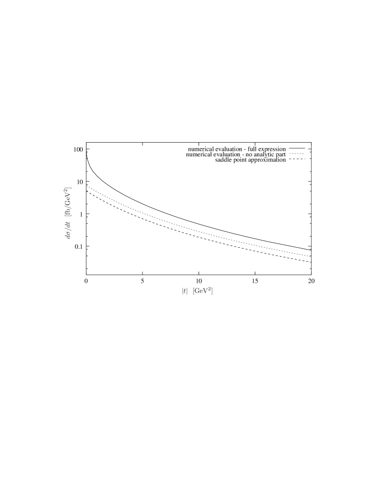
Figure 3: Differential cross section: comparison of two different approximations of the Odderon wave function with the exact result

We find a maximal enhancement factor of the exact calculation over the SPA of order 25 at $t=t_{\mathrm{min}}$, but quickly shrinking with increasing $|t|$ to an enhancement of order 2. For the total cross section the SPA calculation leads to $\sigma^{\mathrm{SPA}}_{\mathrm{tot}}\approx 13\,\mbox{fb}$, hence underestimating the total cross section approximately by a factor 5. So we find that the SPA in its simplest form should not be applied to the scattering process at hand, at least if one is interested in small values of $|t|$.

This result appears surprising at first sight, as it was found that in calculations involving the BFKL Pomeron the saddle point approximation typically overestimates the cross section, the deviation from the actual cross section usually being of the order of $20\,\%$, see for example [38] for the case of the total hadronic cross section in virtual photon collisions. We therefore find it instructive to discuss the origin of the large deviation and its direction in the case of the BLV solution in our process.

As was mentioned in section 2.5, in the SPA the analytic part $E^{(\nu)}_{A}$ of the BFKL eigenfunction is completely neglected. In figure 3 we also show how this affects the $t$-dependence. Going to small $|t|$, the curve resulting from the full calculation (including the analytic part) has a much steeper $t$-dependence than the SPA curve, leading to the large enhancement. We have also included in this figure the cross section obtained by neglecting the analytic part while calculating the $\nu$ integral numerically without the SPA. That curve is very similar to the SPA curve in its $t$-dependence, but is higher by a factor of about 1.5. Thus we see that the crucial difference is not caused by the approximation of the argument of the exponential, but by the fact that the analytic part is neglected.

The omission of the analytic part $E_{A}^{(\nu)}$ in the SPA is due to the fact that the first non-vanishing term in the Taylor expansion (in $\nu$) of $E_{A}^{(\nu)}$ is of second order, whereas the delta function contribution $E_{\delta}^{(\nu)}$ already has a non-vanishing zeroth order term. But as the factor $y$ in the exponent is not very large, the analytic piece nevertheless contributes substantially to the $\nu$ integral. Thus a numerical investigation of the $\nu$-dependence of the different parts of the solution is needed to obtain a clearer picture of the importance of the analytic part.

In figure 4 we show the real and imaginary parts of both contributions to the expression $\langle\phi|E^{(\nu)}\rangle_{u}$ at $|t|=0.01$ GeV².

Figure 4: Comparison of the different contributions to $\langle\phi|E^{(\nu)}\rangle$; the solid line is the Gauss-like function $I(\nu)$ representing the momentum-independent factors of the $\nu$-integrand (the curve is scaled and shifted, see text)

We have not included the constant factors in this calculation, so that the figure shows only the relative size of the different terms. We recall that, before being integrated, the expression $\langle\phi|E^{(\nu)}\rangle_{u}$ gets multiplied with the corresponding lower part and the rest of the $\nu$ integrand in (30). The latter is given by

$$I(\nu)=e^{y\chi(\nu)}\frac{(2\pi)^{2}(\nu^{2}+\frac{1}{4})}{\nu^{2}(\nu^{2}+1)}\frac{b^{2}}{c(\nu)^{2}}$$ (32)

To better understand the significance of a particular contribution to the overall result, we have included in figure 4 also this momentum-independent contribution $I(\nu)$ to the integral (solid curve). It basically gives a Gauss-like-curve with a maximum $I_{0}$ at $\nu=0$. It is scaled and shifted in such a way that the lower horizontal axis in the figure is the $I(\nu)=0$ level and the upper one the $I(\nu)=I_{0}$ level (see r.h.s. of the figure).

It now becomes clear from the figure, why the SPA cannot lead to good results in our calculation. The analytic part (dashed lines) gets comparable in size to the $\delta$-function part (dotted) already at $\nu\approx 0.2$, where the Gauss-like factor (solid line) is still at about 70% of its maximal value. At larger values of $\nu$ the analytic part even contributes dominantly to the amplitude. Compared to the approximated integrand, where the analytic part is neglected but the $\nu$ integration is done numerically (no SPA), this gives an enhancement by a factor of 12 in the differential cross section (which can be understood when keeping in mind that the expression $\langle\phi|E^{(\nu)}\rangle$ gets squared when the result of the lower part is multiplied and again squared when the cross section is calculated). The analytic part falls off much faster with $|t|$ than the $\delta$-function part, so the SPA improves with increasing momentum transfer. For values of $|t|>5\,\mbox{GeV}^{2}$ it reproduces the $t$-dependence fairly well. Nevertheless, even for larger values of $|t|$ the size of the differential cross section is significantly underestimated by the SPA. We find that the analytic part $E_{A}$ becomes negligible at small $t$ only for extremely large $y$ above $\sim 100$.

3.4 Energy and scale dependence of the cross section

The intercept of the BLV solution equals unity, so there should be no power-like energy dependence of the cross section. But as the continuous quantum number $\nu$ of the BLV solution leads to a cut in the complex angular momentum plane (instead of a simple pole), we expect a $\log^{-c(t)}s$ dependence. This can be numerically verified by keeping $t$ fixed and calculating the cross section as a function of $s$. Again, the results of this calculation can be compared to the SPA to check the significance of the latter. The comparison with the noninteracting three-gluon exchange process does not give any new insight, as there is no energy dependence in that cross section.

The saddle point approximation gives an inverse logarithmic dependence on the energy, as can be easily seen when keeping in mind that $s$ only appears in the Gaussian exponential $\exp(-yc^{\prime}\nu^{2})$ in the factor $y=\log(s/s_{0})$ (with $c^{\prime}=2N_{c}\alpha_{s}/\pi$). Similar results are expected for the numerical calculation if this approximation should be reasonable. However, as pointed out in the previous section, in the domain of the momentum transfer that gives the largest contribution to the total cross section (i.e. the small $|t|$ domain) the applicability of the saddle point approximation is very questionable.

Again, we have calculated the differential cross section numerically, this time varying $s$. To the results a function of the form

$$f(s)=a\log^{-b}(s/s_{0})$$ (33)

is fitted with fitting parameters $a$ and $b$ that depend only on $t$. To see the change of the $s$-dependence with varying $t$, we have performed the calculation for $|t|=0.01,0.1,1$ and $10\,\mbox{GeV}^{2}$. The results for a wide range of squared center-of-mass energies $s$ together with the fitted curves are shown in figure 5.

Figure 5: $s$-dependence of the differential cross section for real photons for $|t|=0.01,0.1,1,10\,\mbox{GeV}^{2}$ (top to bottom), the points are numerical results, the lines represent fits (see text)

One can see that the expected behavior is reproduced quite well by the numerical results. This should however not be understood as a possibility to determine the value of $b$ in (33) as a function of $t$. From the fits we get values for $b$ ranging from $1.9$ at $|t|=0.01\,\mbox{GeV}^{2}$ to $2.4$ at $|t|=1\,\mbox{GeV}^{2}$, but in the limit of asymptotically large $s$, all these curves eventually have to approach the saddle point approximation, because it does become valid at some large value of $y$ when the Gaussian factor gets so narrow that only the region of small $\nu$ gives a sizeable contribution to the integrand. Therefore, in the limit $s\to\infty$, we know that $b\to 1$.

In the case of center-of-mass energies accessible at present and planned accelerators (up to $y\approx 10$), however, the fitted curves give a reasonable description of the energy dependence. Again, we find the SPA to be inappropriate for the parameter range of small $|t|$ and realistic $s$. In order to keep the figure readable, we did not include the SPA curves, but again they fail completely in quantitatively reproducing the numerical results. This can be easily seen from the fact that the exponent of the logarithm is determined to be around $b\approx 2$, whereas the SPA gives an exponent $b=1$. It is only at values of $s$ well beyond any realistic size ($y\gg 100$) that the saddle point approximation becomes acceptable already for small $|t|$.

We now turn to the question of the dependence of our results on the choice of the scale $s_{0}$. For all of the previous calculations we had chosen the fixed scale $s_{0}=m_{\eta_{c}}^{2}$ in $y=\log(s/s_{0})$. The scale $s_{0}$ of the energy cannot be determined in LLA since a change in $s_{0}$ is formally sub-leading in the expansion of logarithms. The numerical results, however, do naturally depend on the specific choice. It is therefore interesting to see the influence of different choices of $s_{0}$ on the cross section. If $s$, $t$ and $Q$ are fixed, a change of the scale $s_{0}$ by a factor $d$ clearly has the same effect as replacing $s$ by $s/d$ with fixed scale. It is then straightforward to obtain the resulting cross sections from the results obtained above. As long as the scale $s_{0}$ remains small compared to $s$, the change does not qualitatively alter the results.

Yet, the overall magnitude of the cross section is significantly changed by a change in the scale factor. For example, in comparison with $s_{0}=m_{\eta_{c}}^{2}$ the choice $s_{0}=1\,\mbox{GeV}^{2}$, which is the typical mass scale for hadronic processes, changes the result by an approximately constant factor of about $2/3$. Compared to this uncertainty, the numerical and systematical errors in our calculations are definitely negligible. Strictly speaking, the numerical values of our results should only be taken as an indication for the order of magnitude. The appropriate choice for $s_{0}$ and hence the absolute results could only be determined in a next-to-leading order calculation. The qualitative dependence on the momentum transfer and on the center-of-mass energy, however, is quite stable under changes of the scale factor.

As soon as we consider non-vanishing virtualities of one or both of the photons, the choice of the scale $s_{0}$ becomes even more ambiguous. As the virtuality of the photon provides another momentum scale for the reaction, it is natural to include it into the scale factor. The inclusion of the virtuality in $s_{0}$ will lead to different results for the dependence of the differential cross section on the virtuality of the photons, as will be discussed in more detail in section 3.6.

3.5 Possible realizations of $\eta_{c}$ meson photoproduction

In order to relate our results to phenomenology, we want to give some estimates for the cross section in possible future collider setups. So far, we have been concerned with the process $\gamma\gamma\to\eta_{c}\eta_{c}$ with real photons at the fixed center-of-mass energy $\sqrt{s}=300\,\mbox{GeV}$. That scale was chosen having in mind a later comparison to other works concerning the process $\gamma p\to\eta_{c}p$.

A possible realization of quasidiffractive double $\eta_{c}$ production would be the photon collider option at TESLA. In this section we use the definitions and numbers given in the TESLA design report [39]. From an electron-positron center-of-mass beam energy of $E_{\mathrm{beam}}=500\,\mbox{GeV}$ a beam of real photons with a maximum center-of-mass energy $\sqrt{s}=390\,\mbox{GeV}$ can be produced. However, due to the production mechanism of inverse Compton scattering, the resulting beam is not very narrowly peaked, but has a maximum at about $\sqrt{s}=360\,\mbox{GeV}$ with a width at half maximum of about 15 %. The luminosity for photons with an energy in this peak region is estimated as $L_{\gamma\gamma}=1.1\cdot 10^{34}\mbox{cm}^{-2}\mbox{s}^{-1}$. As the dependence on the momentum transfer at this energy does not give any new insight, we do not show a figure of the differential cross section (the curve looks exactly like figure 2). The total cross section for $\sqrt{s}=360\,\mbox{GeV}$ is $\sigma_{\mathrm{tot}}\approx 55\,\mbox{fb}$. This would lead to a total number of events of the order of $10^{5}$ in five years of continuous running.

Another possibility of realizing the process $\gamma\gamma\to\eta_{c}\eta_{c}$ is directly in electron-positron collisions. Here the process occurs as a subprocess in $e^{+}e^{-}\to e^{+}e^{-}\eta_{c}\eta_{c}$ at high energies. The $\gamma\gamma$ subsystem in such a collision has a continuous spectrum and we have to integrate over the energy fractions. In [34] this calculation was performed in the equivalent photon approximation (see also [40]) for the noninteracting three-gluon exchange process. There, it was much easier to calculate the convolution integral, as the simple solution does not exhibit any energy dependence. Because of the large numerical effort of calculating total cross sections in our approach, we use the results from the previous section to estimate the energy dependence of the total cross section. There we found fairly good fits of the form $\propto\log^{b}(s/s_{0})$ with values of $b$ around 2. Therefore, we approximate the total cross section by

$$\sigma_{\mathrm{tot}}(s)=\sigma_{0}\log^{-2}\left(\frac{s}{s_{0}}\right)\,,$$ (34)

where $\sigma_{0}=5040\,\mbox{fb}$ is determined from the value of $\sigma_{\mathrm{tot}}$ at $\sqrt{s}=300\,\mbox{GeV}$.

The center-of-mass energy $\sqrt{s}$ in the $\gamma\gamma$ subprocess is related to the beam energy $E_{\mathrm{beam}}$ as

$$s=z_{1}z_{2}E^{2}_{\mathrm{beam}}\,,$$ (35)

where $z_{1}$, $z_{2}$ are the fractions of the electron and positron energies carried by the two photons.

In the equivalent photon approximation the energy distribution of the photons is given by the flux-factor $f_{\gamma}(z,Q^{2}_{\mathrm{min}},Q^{2}_{\mathrm{max}})$. For untagged $e^{\pm}$ it reads (for details see equations (23)-(25) in [34]):

$$f_{\gamma}(z)=\frac{\alpha}{2\pi}\left(\frac{1+(1-z)^{2}}{z}\log\frac{(1-z)^{2}E^{2}_{\mathrm{beam}}\Theta^{2}_{\mathrm{max}}}{m^{2}_{e}\,z}\right)\,.$$ (36)

where we use $\Theta^{2}_{\mathrm{max}}=30\,\mbox{mrad}$. The cross section for the process $e^{+}e^{-}\to e^{+}e^{-}\eta_{c}\eta_{c}$, which corresponds to the collision of almost real photons, is given by:

$$\int_{0}^{1}dz_{1}\int_{0}^{1}dz_{2}\,\Theta(s-s_{\mathrm{min}})\,\sigma_{\mathrm{tot}}(s)f_{\gamma}(z_{1})f_{\gamma}(z_{2})\,.$$ (37)

Here $s_{\mathrm{min}}$ denotes the minimal squared center-of-mass energy for the process. Again, $E_{\mathrm{beam}}=500\,\mbox{GeV}$ is used.

If we integrate over the complete domain of possible values for $s$, that is $4m_{\eta_{c}}^{2}<s<E^{2}_{\mathrm{beam}}$ we get a total cross section for the electron-positron scattering process of $\approx 55\,\mbox{fb}$, as opposed to $3.5\,\mbox{fb}$ that was obtained for the simple three-gluon exchange in [34]. However, with a squared center-of-mass energy $s=s_{\mathrm{min}}\equiv 4m_{\eta_{c}}^{2}$ one is clearly not in the high energy limit. In particular, the requirement $s\gg t$ is not met. Therefore, we have performed the calculation again for a minimal squared energy of $10\,s_{\mathrm{min}}$ and obtain for the $e^{+}e^{-}$ total cross section a value of $\sigma_{\mathrm{tot}}\approx 7\,\mbox{fb}$. The large difference between these values comes about because the total photon cross section rises as one goes to small values of $s$. Compared to the value at $\sqrt{s}=300\,\mbox{GeV}$ the total cross section for $\sqrt{s}=s_{\mathrm{min}}$ is larger by a factor of 50.

Stating it very cautiously, we estimate the total cross section of the process $e^{+}e^{-}\to e^{+}e^{-}\eta_{c}\eta_{c}$ to be of the order of $10\,\mbox{fb}$. The planned luminosity at TESLA is $3.4\cdot 10^{34}\mbox{cm}^{-2}\mbox{s}^{-1}$ [39]. The resulting order of magnitude of the number of events is similar as in the case of the photon collider option.

A realistic assessment of the feasibility of a measurement of our process at a future Linear Collider would clearly require a more detailed study of the process including detector cuts and tagging efficiencies. Such a study is beyond the scope of the present paper.

3.6 Virtual photon scattering

So far we have been concerned with the case of real photon scattering. In this section we consider the cross section for virtual photons. For definiteness, we choose a virtuality $Q^{2}=25\,\mbox{GeV}^{2}$, again motivated by the choice in [13]. The comparison of the differential cross section for real and virtual photons is presented in figure 6.

Figure 6: Differential cross section for real and virtual ($Q^{2}=25\,\mbox{GeV}^{2}$) photons for $\sqrt{s}=300\,\mbox{GeV}$.

We would like to point out that now and in the following we are again considering cross sections for $\gamma\gamma$ scattering rather than for the corresponding process in $e^{+}e^{-}$ scattering. We have included in the figure the cross sections for the case of two real photons, one real photon and one virtual photon, and two virtual photons.

In the latter two processes there is an additional natural scale in the process that can be included in the scale factor $s_{0}$. In addition to the choices discussed in section 3.4 this clearly gives another range of reasonable choices. For the case of two real photons we have used again $s_{0}=m_{\eta_{c}}^{2}$, for the processes in which at least one virtual photon is involved, we have chosen $s_{0}=m_{\eta_{c}}^{2}+Q^{2}$. That choice appears natural in particular in the light of the typical energy scales occurring in deep inelastic scattering. In the case of a virtual photon scattering on a real photon, one could also think of using some kind of average momentum scale (for example the geometric or the arithmetic mean). This would change the results only by a factor which is almost independent of $|t|$.

In figure 6 it can be seen that the basic dependence on the squared momentum transfer is qualitatively similar for all three processes, but the absolute size of the result is quite different. The virtuality of a photon leads to a suppression of the differential cross section. If both photons are virtual, the cross section is further suppressed. The relative enhancement of the real photon scattering over the processes including virtual photons decreases with growing $|t|$. This behavior does not come as a surprise if one looks at the reduced impact factor (18)

$$\phi({\bf k,q-k})\propto\frac{(2k^{1}-q)}{Q^{2}+4m_{c}^{2}+(2\mathbf{k}-\mathbf{q})^{2}}\,.$$ (38)

The dominant region for the momentum integration is where the gluon momentum $\mathbf{k}$ is small. For small values of $|t|$ the suppression by the virtuality is therefore basically given by a factor $\approx 1/Q^{2}$. For a value of $|t|$ comparable in size to $Q^{2}$, the suppression is only $\approx 1/2$, and if $|t|\gg Q^{2}$ the effect of the virtuality becomes negligible.

For the total cross section this gives a strong suppression with respect to $Q^{2}$. For one virtual ($Q^{2}=25\,\mbox{GeV}^{2}$) and one real photon, we get a total cross section $\sigma_{\mathrm{tot}}\approx 5\,\mbox{fb}$, for both being virtual $\sigma_{\mathrm{tot}}\approx 1\,\mbox{fb}$ (for both real, the cross section was $\sigma_{\mathrm{tot}}\approx 59\,\mbox{fb}$). The three-gluon approximation leads to cross sections $\sigma_{\mathrm{tot}}\approx 2\,\mbox{fb}$ for one virtual photon and $\sigma_{\mathrm{tot}}\approx 0.2\,\mbox{fb}$ if both photons are virtual. Thus we see that the enhancement of the total cross section of the BLV Odderon over the three-gluon approximation gets amplified when one considers virtual photons.

Next, we want to investigate the dependence of the differential cross section on the virtuality of one photon (figure 7) when the second photon is real. For this we keep $t$ fixed ($|t|=1\,\mbox{GeV}^{2}$) and vary $Q^{2}$ in one impact factor. As was already mentioned above, the results of the numerical calculations depend on the specific choice of $s_{0}$ which can now include the virtuality $Q^{2}$. In that case the $Q^{2}$-dependence of the cross section will strongly be affected by the specific choice of $s_{0}$.

In figure 7 we plot the results for three different calculations: the approximation by three noninteracting gluons and the numerical BLV Odderon calculation with two choices for the scale factor.

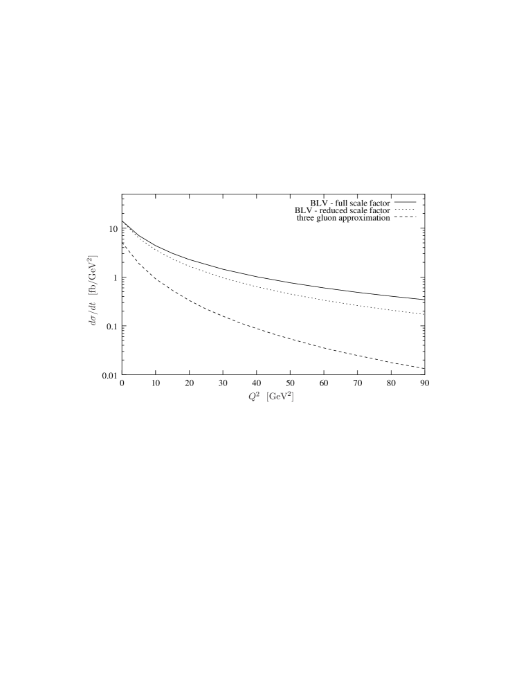
Figure 7: $Q^{2}$-dependence of the differential cross section for one virtual and one real photon at $|t|=1\,\mbox{GeV}^{2}$: comparison of BLV Odderon with two different choices for the scale factor $s_{0}$ and noninteracting three-gluon exchange

These are: the scale that was used in [13], $s_{0}=m_{\eta_{c}}^{2}+Q^{2}$, which we will call ‘full’ scale factor because of the inclusion of the virtuality, and a ‘reduced’ version without the virtuality of the photon, $s_{0}=m_{\eta_{c}}^{2}$. As we have pointed out above, there is no way to determine in LLA which scale choice is the correct one. Consequently the terms ‘full’ and ‘reduced’ are not meant in the sense that the ‘full’ scale factor is ‘better’ in any sense. We see that the reduced scale factor leads to a steeper slope than the full scale factor. Again, we find that the three-gluon approximation exhibits a yet steeper slope with respect to $Q^{2}$. Nevertheless, all curves have a somewhat similar dependence on the virtuality.

A remark is in order here concerning the applicability of the BKP Odderon in the case of a virtual photon scattering on a real one. If the virtuality of the former is large, there is an evolution in transverse momentum along the exchanged gluons in the $t$-channel. The BKP equation, on the other hand, takes into account only evolution in energy but not in transverse momentum. The situation of two largely different photon virtualities would hence require the inclusion of DGLAP type evolution [41, 42, 43] and is not appropriately described by BKP evolution. This limitation of our results for largely different virtualities should be kept in mind when interpreting the results of the present section.

Ignoring that limitation for the moment, we now want to investigate the ‘asymptotic’ $Q^{2}$-dependence. That dependence is of theoretical rather than of phenomenological interest, but can be useful for gaining insight into the BLV Odderon solution. Again we consider the case of one virtual and one real photon. In figures 8 (for the reduced scale factor) and 9 (for the full scale factor) we plot the cross section as a function of $Q^{2}$ for $|t|=0.01$ and $1\,\mbox{GeV}^{2}$. The points are our numerical results, the curves are certain fits on which we will comment below.

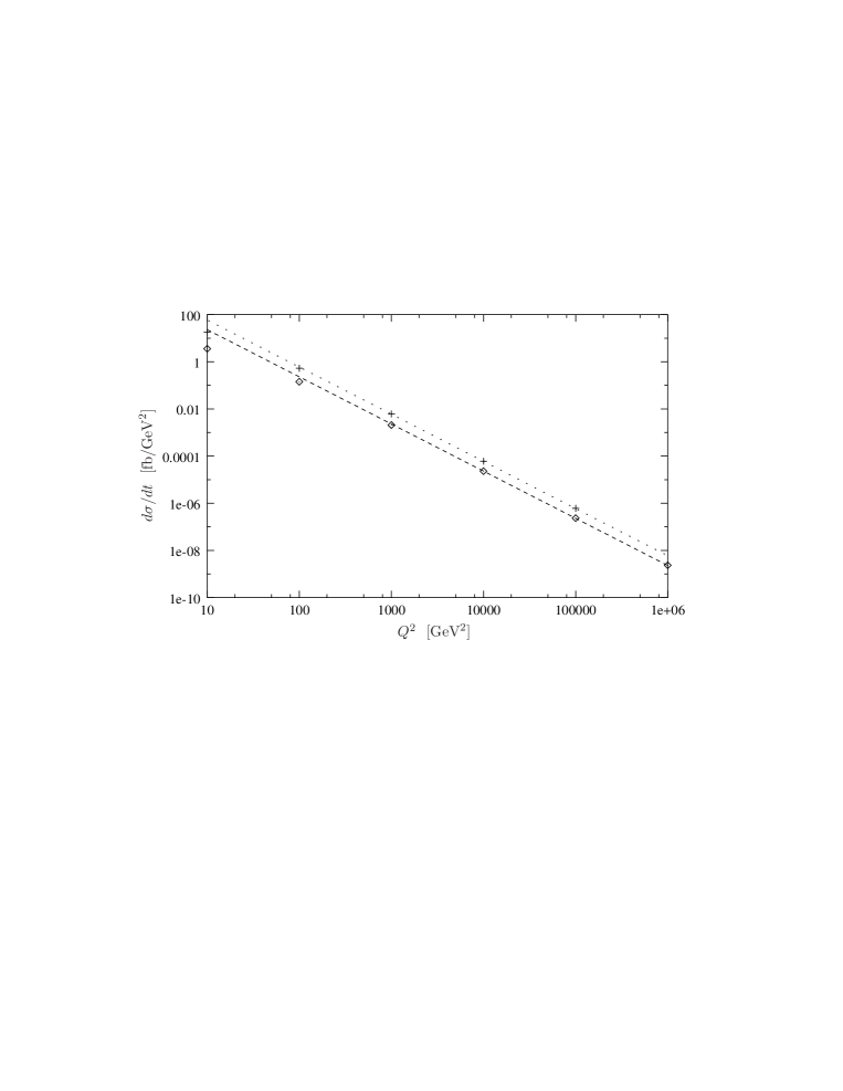
Figure 8: $Q^{2}$-dependence of the differential cross section for one virtual and one real photon, $|t|=0.01\,\mbox{GeV}^{2}$ (upper points) and $|t|=1\,\mbox{GeV}^{2}$ (lower points) with reduced scale factor $s_{0}$; the points are numerical results, the curves are fits (see text)

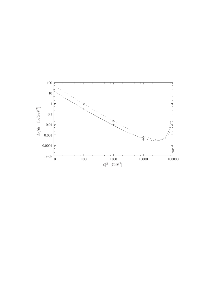
Figure 9: $Q^{2}$-dependence of the differential cross section for one virtual and one real photon, $|t|=0.01\,\mbox{GeV}^{2}$ (upper points) and $|t|=1\,\mbox{GeV}^{2}$ (lower points) with full scale factor $s_{0}$ ($Q^{2}$ included); the points are numerical results, the curves are fits (see text)

If the $Q^{2}$-dependence is not included in $s_{0}$, the result is simple. In the region $m_{c}^{2}\ll Q^{2}\ll s$ we find a ($t$-independent) scaling behavior of the cross section of $\frac{d\sigma}{dt}\propto Q^{-4}$ (the fitted curves in figure 8). This can be easily understood. The virtuality of the incident photon appears explicitly only in the impact factors (38), as the BLV Green function itself does not exhibit a $Q^{2}$-dependence. The momentum integrals $\langle\phi|E^{(\nu)}\rangle$ receive the dominant contribution from the region of small transverse momenta. As long as all momentum components are small compared to $\sqrt{Q^{2}}$, the error we make by pulling the numerator out of the integral as a factor $Q^{-2}$ is small. In the cross section this gives a contribution of $|Q|^{-4}$. We have added to the figures a fit with exactly that $Q^{2}$-dependence to show the agreement with the numerical results.

If we include a $Q^{2}$-dependence in the scale $s_{0}$ via the ‘full’ scale factor $s_{0}=m_{\eta_{c}}^{2}+Q^{2}$, the overall dependence on $Q^{2}$ changes qualitatively. In the domain $m_{\eta_{c}}^{2}\ll Q^{2}\ll s$ we basically expect a curve that resembles the $|Q|^{-4}$ result from the simple choice $s_{0}=m^{2}_{\eta_{c}}$ multiplied by the dependence that we get from section 3.4, $\propto\log^{-b(t)}(s/Q^{2})$. In figure 9 we show the numerical results together with a fit representing that expectation. The fit fails when $Q^{2}$ approaches the boundary of the domain in which it is expected to apply but gives a fairly good description of the slope within that domain. The slope with respect to $\sqrt{Q^{2}}$ is about $3.2$ for $|t|=0.01\,\mbox{GeV}^{2}$ and about $3.0$ for $|t|=1\,\mbox{GeV}^{2}$, indicating that the slope is not entirely independent of $t$.

A remark is in order here concerning the question of the twist of the different solutions to the BKP equation, and in particular of the BLV solution. This issue has been addressed in [44, 45], see also [46]. The twist of the Odderon solutions is an interesting quantity from a theoretical point of view and crucial for a thorough understanding of the different solutions. It should be kept in mind, however, that at high energies (or small Bjorken-$x$) the operator product expansion becomes problematic and eventually breaks down, see for example [47]. Our results illustrate an additional problem of the phenomenological aspects of the Odderon twist. A potential measurement of the Odderon twist is likely to be obscured by the effects of different but theoretically equivalent choices of the energy scale $s_{0}$, at least as long as one works in GLLA.

3.7 Comparison with photon-proton scattering

In [13] the process $\gamma p\to\eta_{c}p$ was studied using the BLV Odderon solution. The coupling of the BLV Odderon to the proton is more complicated than the $\gamma\eta_{c}$ impact factor, and here the reduction of the four-dimensional integral over two transverse momenta is not reduced to a two-dimensional one. One therefore has to make use of the saddle point approximation for a numerical calculation of the cross section. The quality of the saddle point approximation is difficult to assess in that process. A comparison with our process can be helpful in this respect, since there we can compare the SPA with the exact results and are hence able to trace the effects of the approximation. In our calculations we have used kinematical parameters similar to those of [13], and we can therefore hope that our results can give us an idea of what the effects of the exact calculation in $\gamma p\to\eta_{c}p$ can be.

Before we discuss possible implications of our results for the process $\gamma p\to\eta_{c}p$ we want to point out some general differences between the results for that process found in [13] and the results found here for the $\gamma\gamma$ case. As was already found in the approximation of three noninteracting gluons [7, 8] the differential cross section for the process $\gamma p\to\eta_{c}p$ vanishes as $|t|\to 0$. This is due to the coupling of the Odderon to the proton impact factor and is not expected in our scattering process. In addition, the calculation involving the BLV solution leads to a pronounced dip in the cross section at $|t|\approx 0.07\,\mbox{GeV}^{2}$. Also this is due to the coupling of the Odderon to the proton as was pointed out in [13], and such a dip is not expected in $\gamma\gamma\to\eta_{c}\eta_{c}$.

In [13] a sizable difference between the BLV cross section and the exchange of three noninteracting gluons [7, 8] was found in $\gamma^{(*)}p\to\eta_{c}p$. For real photons, the cross section is enhanced by a factor of 5 due to resummation, that is for the BLV solution. We find a much smaller enhancement in our process. In addition, when calculating our process in SPA the results are actually smaller than for three-gluon exchange. Therefore, it appears that in $\gamma p$ scattering the enhancement is caused solely by the coupling of the Odderon to the proton. In the case of virtual photons (with $Q^{2}=25\,\mbox{GeV}^{2}$) the $\gamma p$ calculation in SPA gives an enhancement of the total cross section by one order of magnitude. This means that there is an additional enhancement factor of 2 (as compared to the respective three-gluon calculation) caused by the virtuality of the photon. We find approximately the same additional enhancement factor in the case of one virtual photon in our process.

In section 3.3 we found that for our process the saddle point approximation significantly underestimates the cross section. As the convolution of the Odderon wave function with the $\gamma\eta_{c}$ impact factor in the case of photon-proton scattering was calculated in saddle point approximation, too, it is plausible to expect that using the full numerical calculation also in that process would lead to an additional enhancement that is approximately the square root of the one found here, i. e.  by about a factor 2 for the total cross section. We should point out, however, that it is by no means clear that the saddle point approximation also underestimates the Odderon-proton coupling. Instead, also a completely different behavior of the full 4-dimensional integral is conceivable. It would be important to study this problem in more detail and to determine at least the direction of the effect of the saddle point approximation in that coupling.

4 Conclusions and Outlook

We have studied the quasidiffractive process $\gamma^{(*)}\gamma^{(*)}\to\eta_{c}\eta_{c}$ at high energies which is mediated by the exchange of an Odderon. This process is considered to be the theoretically cleanest probe of the Odderon in perturbative QCD since it does not involve the uncertainties typically associated with the coupling of the Odderon to a proton. We have taken into account the effects of resummation of large logarithms of the energy by using the BLV Odderon solution. This is the only solution of the BKP equation which couples in leading order to the $\gamma\eta_{c}$ impact factor.

We have investigated in detail the effect of resummation in this process by comparing our results to the exchange of three noninteracting gluons which is the simplest possible model for a perturbative Odderon. For real photons we find that resummation strongly enhances the differential cross section at small $|t|$, but leads to a faster decrease with increasing $|t|$. The total cross section is consequently only slightly enhanced due to resummation. The enhancement due to resummation is more pronounced when one considers virtual photons. We find a logarithmic decrease of the cross section with the energy in agreement with the intercept of the BLV solution being exactly one. We have discussed in detail the effects of different possible choices for the energy scale $s_{0}$ which is undetermined in leading logarithmic approximation. We have investigated this uncertainty and find that the cross section is rather sensitive to the choice of the energy scale, in particular in the case of virtual photons when the scale $s_{0}$ can naturally involve also the virtuality of the photons.

We have estimated the expected event rates for the process $\gamma\gamma\to\eta_{c}\eta_{c}$ at a future Linear Collider for $e^{+}e^{-}$ scattering as well as for a photon collider option. In both cases the observation of the Odderon in this process appears feasible, but more detailed studies accounting for detector cuts and tagging efficiencies will be required to obtain a conclusive assessment of this process.

All previous phenomenological studies of the BLV Odderon solution were done for processes involving protons. Due to the complicated Odderon-proton coupling the numerical effort for an exact calculation of the cross section is prohibitively large in these cases. These processes have therefore been studied in the saddle point approximation. In our process a considerable simplification occurs due to the special structure of the $\gamma\eta_{c}$ impact factor and an exact numerical calculation becomes possible. We have used our exact results to test the quality of the saddle point approximation in our process. We find that for realistic values of the kinematical parameters the saddle point approximation fails and underestimates the actual cross section by about an order of magnitude. We have identified the origin of this large deviation and have indicated possible implications of our result for processes in which the BLV Odderon solution is coupled to a proton.

Finally, we would like to point out that also other final states can be produced via Odderon exchange in quasidiffractive photon-photon scattering. An interesting example among them is the single-inclusive process $\gamma\gamma\to\eta_{c}X$ which can be treated in a similar way as the process discussed in the present paper. In that process, however, the situation is similar to the processes in which the BLV Odderon is coupled to a proton. The coupling of the BLV Odderon to the $\gamma X$ impact factor does not allow one to reduce the four-dimensional integral over transverse momenta to a two-dimensional one. An exact numerical evaluation of the integral is therefore not feasible and again one has to make use of the saddle point approximation. In the light of our results, however, it seems likely that also here that approximation gives only a relatively poor estimate of the actual cross section. Despite this difficulty it would be very interesting to study the effects of resummation also in $\gamma\gamma\to\eta_{c}X$ and in related processes involving tensor mesons in more detail since they might offer a good chance to observe the Odderon.

References

- [1] L. Lukaszuk and B. Nicolescu, Lett. Nuovo Cim. 8 (1973) 405.
- [2] A. Breakstone et al., Phys. Rev. Lett. 54 (1985) 2180.
- [3] C. Ewerz, arXiv:hep-ph/0306137.
- [4] A. Schäfer, L. Mankiewicz and O. Nachtmann, Phys. Lett. B 272 (1991) 419.
- [5] V. V. Barakhovsky, I. R. Zhitnitsky and A. N. Shelkovenko, Phys. Lett. B 267 (1991) 532.
- [6] A. Schäfer, L. Mankiewicz and O. Nachtmann, in Proc. of the Workshop ”Physics at HERA”, Hamburg 1991, vol. 1, p. 243.
- [7] J. Czyzewski, J. Kwieciński, L. Motyka and M. Sadzikowski, Phys. Lett. B 398 (1997) 400 [Erratum-ibid. B 411 (1997) 402] [arXiv:hep-ph/9611225].
- [8] R. Engel, D. Y. Ivanov, R. Kirschner and L. Szymanowski, Eur. Phys. J. C 4 (1998) 93 [arXiv:hep-ph/9707362].
- [9] M. G. Ryskin, Eur. Phys. J. C 2 (1998) 339.
- [10] W. Kilian and O. Nachtmann, Eur. Phys. J. C 5 (1998) 317 [arXiv:hep-ph/9712371].
- [11] E. R. Berger, A. Donnachie, H. G. Dosch, W. Kilian, O. Nachtmann and M. Rueter, Eur. Phys. J. C 9 (1999) 491 [arXiv:hep-ph/9901376].
- [12] E. R. Berger, A. Donnachie, H. G. Dosch and O. Nachtmann, Eur. Phys. J. C 14 (2000) 673 [arXiv:hep-ph/0001270].
- [13] J. Bartels, M. A. Braun, D. Colferai and G. P. Vacca, Eur. Phys. J. C 20 (2001) 323 [arXiv:hep-ph/0102221].
- [14] J. Bartels, M. A. Braun and G. P. Vacca, arXiv:hep-ph/0304160.
- [15] J. P. Ma, Nucl. Phys. A 727 (2003) 333 [arXiv:hep-ph/0301155].
- [16] S. J. Brodsky, J. Rathsman and C. Merino, Phys. Lett. B 461 (1999) 114 [arXiv:hep-ph/9904280].
- [17] I. P. Ivanov, N. N. Nikolaev and I. F. Ginzburg, in Proc. 9th International Workshop on Deep Inelastic Scattering (DIS 2001), Bologna, Italy, 2001, arXiv:hep-ph/0110181.
- [18] P. Hägler, B. Pire, L. Szymanowski and O. V. Teryaev, Phys. Lett. B 535 (2002) 117 [Erratum-ibid. B 540 (2002) 324] [arXiv:hep-ph/0202231].
- [19] P. Hägler, B. Pire, L. Szymanowski and O. V. Teryaev, Eur. Phys. J. C 26 (2002) 261 [arXiv:hep-ph/0207224].
- [20] I. F. Ginzburg, I. P. Ivanov and N. N. Nikolaev, Eur. Phys. J. directC 5 (2003) 02 [arXiv:hep-ph/0207345].
- [21] C. Adloff et al. [H1 Collaboration], Phys. Lett. B 544 (2002) 35 [arXiv:hep-ex/0206073].
- [22] H. G. Dosch, Phys. Lett. B 190 (1987) 177.
- [23] H. G. Dosch and Y. A. Simonov, Phys. Lett. B 205 (1988) 339.
- [24] Y. A. Simonov, Nucl. Phys. B 307 (1988) 512.
- [25] O. Nachtmann, Annals Phys. 209 (1991) 436.
- [26] H. G. Dosch, C. Ewerz and V. Schatz, Eur. Phys. J. C 24 (2002) 561 [arXiv:hep-ph/0201294].
- [27] J. Bartels, Nucl. Phys. B 175 (1980) 365.
- [28] J. Kwieciński and M. Praszałowicz, Phys. Lett. B 94 (1980) 413.
- [29] R. A. Janik and J. Wosiek, Phys. Rev. Lett. 82 (1999) 1092 [arXiv:hep-th/9802100].
- [30] J. Bartels, L. N. Lipatov and G. P. Vacca, Phys. Lett. B 477 (2000) 178 [arXiv:hep-ph/9912423].
- [31] Y. V. Kovchegov, L. Szymanowski and S. Wallon, arXiv:hep-ph/0309281.
- [32] I. F. Ginzburg, D. Y. Ivanov and V. G. Serbo, Phys. Atom. Nucl. 56 (1993) 1474 [Yad. Fiz. 56N11 (1993) 45].
- [33] I. F. Ginzburg and D. Y. Ivanov, Nucl. Phys. Proc. Suppl. 25B (1992) 224.
- [34] L. Motyka and J. Kwieciński, Phys. Rev. D 58 (1998) 117501 [arXiv:hep-ph/9802278].
- [35] E. A. Kuraev, L. N. Lipatov and V. S. Fadin, Sov. Phys. JETP 45 (1977) 199 [Zh. Eksp. Teor. Fiz. 72 (1977) 377].
- [36] I. I. Balitsky and L. N. Lipatov, Sov. J. Nucl. Phys. 28 (1978) 822 [Yad. Fiz. 28 (1978) 1597].
- [37] L. N. Lipatov, Sov. Phys. JETP 63 (1986) 904 [Zh. Eksp. Teor. Fiz. 90 (1986) 1536].
- [38] J. Bartels, A. De Roeck and H. Lotter, Phys. Lett. B 389 (1996) 742 [arXiv:hep-ph/9608401].
- [39] B. Badelek et al. [ECFA/DESY Photon Collider Working Group Collaboration], “TESLA Technical Design Report, Part VI, Chapter 1: Photon collider at TESLA,” arXiv:hep-ex/0108012.
- [40] P. Aurenche et al., “Gamma-Gamma Physics at LEP2,” arXiv:hep-ph/9601317.
- [41] V. N. Gribov and L. N. Lipatov, Sov. J. Nucl. Phys. 15 (1972) 438 [Yad. Fiz. 15 (1972) 781].
- [42] G. Altarelli and G. Parisi, Nucl. Phys. B 126 (1977) 298.
- [43] Y. L. Dokshitzer, Sov. Phys. JETP 46 (1977) 641 [Zh. Eksp. Teor. Fiz. 73 (1977) 1216].
- [44] H. J. de Vega and L. N. Lipatov, Phys. Rev. D 66 (2002) 074013 [arXiv:hep-ph/0204245].
- [45] G. P. Korchemsky, J. Kotanski and A. N. Manashov, Phys. Lett. B 583 (2004) 121 [arXiv:hep-ph/0306250].
- [46] A. G. Shuvaev, arXiv:hep-ph/0310344.
- [47] A. H. Mueller, Phys. Lett. B 396 (1997) 251 [arXiv:hep-ph/9612251].