DESY 04–047 hep-ph/0403192
SFB/CPP-04-09
NIKHEF 04-001
March 2004

The Three-Loop Splitting Functions in QCD:
The Non-Singlet Case
S. Moch${}^{\,a}$, J.A.M. Vermaseren${}^{\,b}$ and A. Vogt${}^{\,b}$
^aDeutsches Elektronensynchrotron DESY
Platanenallee 6, D–15735 Zeuthen, Germany
^bNIKHEF Theory Group
Kruislaan 409, 1098 SJ Amsterdam, The Netherlands

Abstract

We compute the next-to-next-to-leading order (NNLO) contributions to the three splitting functions governing the evolution of unpolarized non-singlet combinations of quark densities in perturbative QCD. Our results agree with all partial results available in the literature. We find that the correct leading logarithmic (LL) predictions for small momentum fractions $x$ do not provide a good estimate of the respective complete results. A new, unpredicted LL contribution is found for the colour factor $d^{abc\,}d_{abc}$ entering at three loops for the first time. We investigate the size of the corrections and the stability of the NNLO evolution under variation of the renormalization scale. Except for very small $x$ the corrections are found to be rather small even for large values of the strong coupling constant, in principle facilitating a perturbative evolution into the sub-GeV regime.

1 Introduction

Parton distributions form indispensable ingredients for the analysis of all hard-scattering processes involving initial-state hadrons. The dependence of these quantities on the fraction $x$ of the hadron momentum carried by the quark or gluon cannot be calculated in perturbation theory. However, the scale-dependence (evolution) of the parton distributions can be derived from first principles in terms of an expansion in powers of the strong coupling constant $\alpha_{\rm s}$. The corresponding $n\,$th-order coefficients governing the evolution are referred to as the $n$-loop anomalous dimensions or splitting functions. Parton densities evolved by including the terms up to order $\alpha_{\rm s}^{\,n+1}$ in this expansion constitute, together with the corresponding results for the partonic cross sections for the observable under consideration, the NⁿLO (leading-order, next-to-leading-order, next-to-next-to-leading-order, etc.) approximation of perturbative QCD.

Presently the next-to-leading-order is the standard approximation for most important processes. The corresponding one- and two-loop splitting functions have been known for a long time [1, 2, 3, 4, 5, 6, 7, 8, 9, 10, 11]. The NNLO corrections need to be included, however, in order to arrive at quantitatively reliable predictions for hard processes at present and future high-energy colliders. These corrections are so far known only for structure functions in deep-inelastic scattering [12, 13, 14, 15] and for Drell-Yan lepton-pair and gauge-boson production in proton–(anti-)proton collisions [16, 17, 18, 19] and the related cross sections for Higgs production in the heavy-top-quark approximation [17, 20, 21, 22]. Work on NNLO cross sections for jet production is under way and expected to yield results in the near future, see Ref. [23] and references therein. For the corresponding three-loop splitting functions, on the other hand, only partial results have been obtained up to now, most notably the lowest six/seven (even or odd) integer-$N$ Mellin moments [24, 25, 26].

These Mellin moments already provide a rather accurate description of the splitting functions at large momentum fractions $x$ [25, 27, 28, 29]. Their much-debated behaviour at small values of $x$, on the other hand, can only be determined by a full calculation. As we will demonstrate below for the non-singlet cases, this statement holds despite the existence of resummation predictions for the leading small-$x$ logarithms [30, 31], since –a– the correctly predicted logarithms do not dominate the three-loop splitting functions at any practically relevant value of $x$ and –b– a term of the same size occurs with a new colour factor at third order which could not have been predicted from lower-order results, analogous to the situation for the four-loop $\beta$-function of QCD [32].

In this article we present the (unpolarized) flavour non-singlet (ns) splitting functions at the third order in perturbative QCD. The corresponding flavour singlet results will appear in a forthcoming publication [33]. The present article is organized as follows: In section 2 we set up our notations for the three independent third-order splitting functions and briefly discuss the method of our calculation. The Mellin-$N$ space results are written down in section 3 together with their explicit large-$N$ limit which is relevant for the soft-gluon threshold resummation [34, 35, 36] at next-to-next-to leading logarithmic accuracy [37]. A surprising relation is found between the leading large-$N$ term at two loops and the subleading $(\ln N)/N$ contribution at third order. In section 4 we present the exact results as well as compact parametrizations for the $x$-space splitting functions and study their behaviour at small $x$. The numerical implications of these results for the scale dependence of the non-singlet quark distributions are illustrated in section 5. Except for very small values of $x$, the perturbation series appears to be well-behaved even down to sub-GeV scales where the initial distributions have been studied using non-perturbative methods for example in Refs. [38, 39, 40, 41, 42, 43]. Finally we briefly summarize our findings in section 6.

2 Notations and method

We start by setting up our notations for the non-singlet combinations of parton distributions and the splitting functions governing their evolution. The number distributions of quarks and antiquarks in a hadron are denoted by $q_{i}(x,\mu_{f}^{\,2})$ and $\bar{q}_{i}(x,\mu_{f}^{\,2})$, respectively, where $x$ represents the fraction of the hadron momentum carried by the parton and $\mu_{f}$ stand for the factorization scale. There is no need to introduce a renormalization scale $\mu_{r}$ different from $\mu_{f}$ at this point. The subscript $i$ indicates the flavour of the (anti-)quark, with $i=1,\ldots,{n_{\!f}}\,$ for ${n_{\!f}}$ flavours of light quarks.

The general structure of the (anti-)quark (anti-)quark splitting functions, constrained by charge conjugation invariance and flavour symmetry, is given by

$$P_{{\rm q}_{i}{\rm q}_{k}}\>=\>P_{\bar{{\rm q}}_{i}\bar{{\rm q}}_{k}} \!=\! \delta_{ik}P_{{\rm q}{\rm q}}^{\,\rm v}+P_{{\rm q}{\rm q}}^{\,\rm s}$$

$$P_{{\rm q}_{i}\bar{{\rm q}}_{k}}\>=\>P_{\bar{{\rm q}}_{i}{\rm q}_{k}} \!=\! \delta_{ik}P_{{\rm q}\bar{{\rm q}}}^{\,\rm v}+P_{{\rm q}\bar{{\rm q}}}^{\,\rm s}\>\>.$$ (2.1)

In the expansion in powers of $\alpha_{\rm s}$ the flavour-diagonal (‘valence’) quantity $P_{\rm qq}^{\,\rm v}$ starts at first order, while $P_{{\rm q}\bar{{\rm q}}}^{\,\rm v}$ and the flavour-independent (‘sea’) contributions $P_{{\rm qq}}^{\,\rm s}$ and $P_{{\rm q}\bar{{\rm q}}}^{\,\rm s}$ are of order $\alpha_{\rm s}^{2}$. A non-vanishing difference $P_{{\rm qq}}^{\,\rm s}-P_{{\rm q}\bar{{\rm q}}}^{\,\rm s}$ occurs for the first time at the third order.

This general structure leads to three independently evolving types of non-singlet distributions: The evolution of the flavour asymmetries

$$q_{{\rm ns},ik}^{\,\pm}\>=\>q_{i}\pm\bar{q}_{i}-(q_{k}\pm\bar{q}_{k})$$ (2.2)

and of linear combinations thereof, hereafter generically denoted by $q_{\rm ns}^{\pm}$, is governed by

$$P_{\rm ns}^{\,\pm}\>=\>P_{{\rm q}{\rm q}}^{\,\rm v}\pm P_{{\rm q}\bar{{\rm q}}}^{\,\rm v}\>\>.$$ (2.3)

The sum of the valence distributions of all flavours,

$$q_{\rm ns}^{\rm v}\>=\>\sum_{r=1}^{{n_{\!f}}}(q_{r}-\bar{q}_{r})\>\>,$$ (2.4)

evolves with

$$P_{\rm ns}^{\,\rm v}\>=\>P_{\rm qq}^{\,\rm v}-P_{{\rm q}\bar{{\rm q}}}^{\,\rm v}+{n_{\!f}}(P_{\rm qq}^{\,\rm s}-P_{{\rm q}\bar{{\rm q}}}^{\,\rm s})\>\equiv\>P_{\rm ns}^{\,-}+P_{\rm ns}^{\,\rm s}\>\>.$$ (2.5)

The first moments of $P_{\rm ns}^{-}$ and $P_{\rm ns}^{\,\rm v}$ vanish, since the first moments of the distributions $q_{\rm ns}^{-}$ and $q_{\rm ns}^{\rm v}$ reflect conserved additive quantum numbers.

We expand the splitting functions in powers of $a_{\rm s}\,\equiv\,\alpha_{\rm s}/(4\pi)$, i.e. the evolution equations for $q_{\rm ns}^{\>i}(x,\mu_{f}^{\,2})$, $i=\pm,{\rm v},$ are written as

$$\frac{d}{d\ln\mu_{f}^{\,2}}\>q_{\rm ns}^{\>i}(x,\mu_{f}^{\,2})\>=\>\sum_{n=0}\>\left(\frac{\alpha_{\rm s}(\mu_{f}^{\,2})}{4\pi}\right)^{\!n+1}P_{\rm ns}^{\,(n)i}(x)\,\otimes\,q_{\rm ns}^{\,i}(x,\mu_{f}^{\,2})$$ (2.6)

where $\otimes$ represents the standard Mellin convolution.

Our calculation is preformed in Mellin-$N$ space, i.e., we compute the non-singlet anomalous dimensions $\gamma_{\,\rm ns}^{\,(n)i}(N)$ which are related by the Mellin transformation

$$\gamma_{\,\rm ns}^{\>(n)i}(N)\>=\>-\int_{0}^{1}\!dx\>\,x^{\,N-1}\,P_{\,\rm ns}^{\,(n)i}(x)$$ (2.7)

to the splitting functions discussed above. The relative sign is the standard convention. Note that in the older literature an additional factor of two is often included in Eq. (2.7).

The calculation follows the methods of Refs. [24, 25, 26, 44, 45]. We employ the optical theorem and the operator product expansion to calculate Mellin moments of the deep-inelastic structure functions. Since we treat the Mellin moment $N$ as an analytical parameter, we cannot apply the techniques of Refs. [24, 25, 26], where the Mincer program [46, 47] was used as the tool to solve the integrals. Instead, the introduction of new techniques was necessary, and various aspects of those have already been discussed in Refs. [45, 48, 49, 50]. Here we briefly summarize our approach, focussing on some parts which have not been presented yet. It should be emphasized that we have at our disposal a very powerful check on all our derivations and calculations by letting, at any point, $N$ be some positive integer value. Then we can resort to the approach of Refs. [24, 25, 26] and, with the help of the Mincer program, the checking of all programs greatly simplifies.

We start by constructing the diagrams for the forward Compton reactions

$$\mbox{quark}\,(P)+\mbox{vector}\,(Q)\>\longrightarrow\>\mbox{quark}\,(P)+\mbox{vector}\,(Q)\>\>,$$ (2.8)

which contribute to the non-singlet structure functions $F_{2}$, $F_{L}$ and $F_{3}$ of deep-inelastic scattering. The $N$-th Mellin moment is given by the $N$-th derivative with respect to the quark momentum $P$ at $P=0$. The diagrams are generated automatically with the diagram generator Qgraf [51] and for all symbolic manipulations we use the latest version of Form [52, 53]. The calculation is performed in dimensional regularization [54, 55, 56, 57] with $D=4-2\epsilon$. The unrenormalized results in Mellin space are formulae in terms of the invariants determined by the colour group [58], harmonic sums [6, 7, 59, 60, 61] and the values $\zeta_{3}$, $\zeta_{4}$, $\zeta_{5}$ of the Riemann $\zeta$-function. In physics results the terms with $\zeta_{4}$ cancel in $N$-space. With the help of an inverse Mellin transformation the results can be transformed to harmonic polylogarithms [62, 63, 64] in Bjorken-$x$ space. Details have been discussed in Refs. [45, 65]. The renormalization is carried out in the $\overline{\mbox{MS}}$-scheme [66, 67] as described in Ref. [24, 25, 26].

The complete non-singlet contributions to the structure functions can be obtained from three Lorentz projections of the amplitude for the process (2.8), that is with $g^{\mu\nu}$, $P^{\mu}P^{\nu}$ and with $\epsilon^{PQ\mu\nu}\equiv\epsilon^{\alpha\beta\mu\nu}P_{\alpha}Q_{\beta}$. For the projection with $g^{\mu\nu}$ and $P^{\mu}P^{\nu}$ one has two vector-like couplings, whereas for the projection with $\epsilon^{PQ\mu\nu}$ one has the product of a vector and an axial-vector coupling. The axial nature leads to the need for additional renormalizations with $Z_{A}$, the axial renormalization, and with $Z_{5}$, the finite renormalization due to the treatment of the $\gamma_{5}$. This is all described in the literature [68]. For the anomalous dimensions we need only the divergent parts of the $g^{\mu\nu}$ and $\epsilon^{PQ\mu\nu}$ projections, but just as for the fixed moments we can also obtain the finite pieces which lead to the coefficient functions in N³LO. The determination of the latter for $F_{2}$ and $F_{L}$ requires also the computation of the $P^{\mu}P^{\nu}$ projection which is still in progress. The results for the three-loop coefficient functions will thus be presented in a future publication [69].

To solve the integrals we apply the following strategy [45, 49]. We set up a hierarchy of classes among all diagrams depending on the topology, for instance ladder, Benz or non-planar. Within a certain topology, we define a sub-hierarchy depending on the number of $P$-dependent propagators. We define basic building blocks (BBB’s) as diagrams of a given topology in which the quark momentum $P$ flows only through a single line in the diagram, while composite building blocks (CBB’s) denote all diagrams with more than one $P$-dependent propagator. We determine reduction schemes that map the CBB’s of a given topology class to the BBB’s of the same topology class or to simpler CBB topologies. Subsequently, we use reduction identities that express the BBB’s of a given topology class in terms of BBB’s of simpler topologies.

This procedure has been discussed to some extent in Refs. [45, 49]. It exploits various categories of relations between the integrals which can be derived as follows. For a generic loop integral depending on external momenta $P$ and $Q$, the first category are integration-by-parts identities [54, 70],

$$\int\,\prod_{n}\,d^{D}p_{n}\,{\partial\over\partial p_{i}^{\,\mu}}\,p_{j}^{\,\mu}\>\times\>(\dots) = 0\,.$$ (2.9)

These give a number of nontrivial relations by making various choices for the $p_{i}$ and $p_{\!j}$ from the loop momenta. Additionally $p_{\!j}$ can be equal to $P$ or $Q$. The second category is based on scaling arguments [45] in Mellin space. They involve applying one of the operators

$$Q^{\,\mu}{\partial\over\partial Q^{\,\mu}}\>\>,\quad\quad\quad P^{\,\mu}{\partial\over\partial Q^{\,\mu}}\>\>,\quad\quad\quad P^{\,\mu}{\partial\over\partial P^{\,\mu}}$$ (2.10)

both inside the integral and to the integrated result. The scaling in Mellin space tells us the effect of these operators on the integrated result, while inside the integral we just work out the derivative. These relations naturally involve polynomials linear in $N$. The fourth operator of this kind,

$$Q^{\mu}{\partial\over\partial P^{\mu}}\>\>,$$ (2.11)

cannot be used naively in this context, because it does not commute with the limit $P\!\cdot\!P\to 0$. More care is needed in this case and we will come back to this shortly.

A third category of relations is obtained along the lines of the Passarino–Veltman decomposition into form factors [71]. In Mellin space we write

$$\int\,\prod_{n}\,d^{D}p_{n}\,p_{i}^{\,\mu}\,\times\,(\dots) = Q^{\,\mu}\,I_{Q}+P^{\,\mu}\,I_{P}\,\>\>,$$ (2.12)

where $I_{Q}$ and $I_{P}$ are the two form factors. By contracting Eq. (2.12) either with $Q_{\mu}$ or $P_{\mu}$, the $I_{Q}$ and $I_{P}$ are determined in terms of a number of integrals. Next, by taking the derivative with respect to $Q_{\mu}$, the relevant identities can be obtained. Because the momentum $p_{i}$ can be any of the loop momenta, Eq. (2.12) gives us as many relations as there are loops. Again, in Mellin space, these relations contain polynomials linear in $N$.

The fourth and the fifth category of relations are new. Together with the form factor relations from Eq. (2.12) they were crucial in setting up the reduction scheme for the three-loop topologies. They are based on operators that do not commute with the limit $P\!\cdot\!P\to 0$. In the fourth category, one considers the dimensionless operators

$$O_{1} = {P\cdot Q\over Q\cdot Q}\>Q^{\mu}{\partial\over\partial P^{\mu}}\,,$$ (2.13)

$$O_{2} = {P\cdot Q}\>\>{\partial\over\partial P^{\mu}}\,{\partial\over\partial Q^{\mu}}\,,$$ (2.14)

$$O_{3} = {(P\cdot Q)^{2}\over Q\cdot Q}\>{\partial\over\partial P^{\mu}}\,{\partial\over\partial P^{\mu}}\>\>.$$ (2.15)

Each individual operator $O_{i}$ does not commute with the limit $P\cdot P\to 0$, but certain linear combinations of the $O_{i}$ do. However, one has to extend the ansatz based on scaling arguments in $N$-space. Specifically, one has for the $N$-th moment of an integral $I(N)$

$$I(N) = \bigg{(}{2P\cdot Q\over Q\cdot Q}\bigg{)}^{N}\,(Q\cdot Q)^{\alpha}\,C^{(0)}_{N}+\bigg{(}{2P\cdot Q\over Q\cdot Q}\bigg{)}^{N-2}\,{P\cdot P\over Q\cdot Q}\,(Q\cdot Q)^{\alpha}\,C^{(2)}_{N}\,+\,\dots\>\>,$$ (2.16)

where the $C^{(0)}_{N}$ and $C^{(2)}_{N}$ are dimensionless functions of $N$, and $\alpha$ adjusts the mass dimensions. The novel feature is here the term $C^{(2)}_{N}$ proportional to $P\cdot P$, which one may call higher twist. In contrast, for the relations based on Eq. (2.10) it was sufficient to restrict the ansatz to $C^{(0)}_{N}$.

Applying the differential operators $O_{i}$ in Eqs. (2.13) – (2.15) to the ansatz (2.16), one finds that the combinations

$$2(\alpha+1-N)O_{1}-O_{2}\>\>,\quad\quad\quad(2N-4+D)O_{1}-O_{3}$$ (2.17)

do commute with the limit $P\!\cdot\!P\to 0$. That is to say, any dependence on the higher twist term $C^{(2)}_{N}$ vanishes in this limit and one is left with only contributions from $C^{(0)}_{N}$. Eq. (2.17) adds two more relations, which in Mellin space contain quadratic polynomials in $N$ due to the differential operators of second order. We have checked that differential operators of yet a higher order in $P$ and $Q$ do not add any new information.

Finally, the fifth category of relations again uses the form factor approach of Eq. (2.12). However, now we do not take the derivative with respect to $Q_{\mu}$ but with respect to $P_{\mu}$. Some extra book-keeping is needed here, since one has to take along terms proportional to $P\!\cdot\!P$. Let us write Eq. (2.12) as

$$p_{i}^{\,\mu}\,I = Q^{\,\mu}\,I_{Q}+P^{\,\mu}\,I_{P}\>\>.$$ (2.18)

Taking the derivative of Eq. (2.18) with respect to $P_{\mu}$ in $N$-space one finds

$${\partial\over\partial P^{\mu}}\,p_{i}^{\,\mu}\,I = Q^{\,\mu}\,{\partial\over\partial P^{\,\mu}}\,I_{Q}+(D+N-1)\,I_{P}\>\>.$$ (2.19)

Solving Eq. (2.18) for $I_{Q}$ and $I_{P}$ as above, however keeping all terms $P\!\cdot\!P$, substituting into Eq. (2.19) and finally taking the limit $P\!\cdot\!P\to 0$, we find

$${\partial\over\partial P^{\mu}}\,p_{i}^{\,\mu}\,I = {P\cdot p_{i}\over P\cdot Q}\>Q^{\,\mu}\,{\partial\over\partial P^{\,\mu}}\,I+(D+N-2)\,{Q\cdot p_{i}\,P\cdot Q-Q\cdot Q\,P\cdot p_{i}\over(P\cdot Q)^{2}}\,I\>\>.$$ (2.20)

Again, as the momentum $p_{i}$ can be any of the loop momenta, Eq. (2.20) gives us as many relations with polynomials linear in $N$ as there are loops.

Taken together, the reductions of category one to five suffice to obtain a complete reduction scheme. In particular, the reduction equations of category two to five involve explicitly the parameter $N$ of the Mellin moment. They give rise to difference equations in $N$ for an integral $I(N)$,

$$a_{0}(N)\,I(N)+a_{1}(N)\,I(N-1)+\ldots+a_{m}(N)\,I(N-m)\>=\>G(N)\>\>,$$ (2.21)

in which the function $G$ refers to a combination of integrals of simpler topologies. Zeroth order equations are of course trivial, although sometimes the function $G$ can contain thousands of terms. First order difference equations can be solved analytically in a closed form, introducing one sum. Higher order difference equations on the other hand can be solved constructively, sometimes with considerable effort, by making an ansatz for the solution in terms of harmonic sums. For the present calculation we had to go up to fourth order for certain types of integrals.

Due to the difference equations, which have to be solved in a successive way, a strict hierarchy for topology classes is introduced in the reduction scheme. For a given integral $I$, a difference equation as in Eq. (2.21), with some (often lenghty) function $G$ expressed in terms of harmonic sums, can be solved in terms of harmonic sums again. Subsequently, the result for $I$ can be part of the inhomogenous term in a difference equation for another, more complicated integral. This requires the tabulation of a large number CBB and BBB integrals, because each integral is typically used many times, thus it saves computer time and disk space. Only this tabulation, which required the addition of features to Form [53], renders the calculation feasible with current computing resources. For the complete project, including Refs. [33, 69], we have collected tablebases with more than $100.000$ integrals and a total size of tables of more than 3 GByte.

3 Results in Mellin space

Here we present the anomalous dimensions $\gamma^{\,\pm,{\rm s}}_{\,\rm ns}(N)$ in the $\overline{\mbox{MS}}$-scheme up to the third order in the running coupling constant $\alpha_{\rm s}$, expanded in powers of $\alpha_{\rm s}/(4\pi)$. These quantities can be expressed in terms of harmonic sums [6, 7, 59, 60]. Following the notation of Ref. [59], these sums are recursively defined by

$$S_{\pm m}(M)\>=\>\sum_{i=1}^{M}\>\frac{(\pm 1)^{m}}{i^{\,m}}$$ (3.1)

and

$$S_{\pm m_{1},m_{2},\ldots,m_{k}}(M)\>=\>\sum_{i=1}^{M}\>\frac{(\pm 1)^{m_{1}}}{i^{\,m_{1}}}\>S_{m_{2},\ldots,m_{k}}(i)\>\>.$$ (3.2)

The sum of the absolute values of the indices $m_{k}$ defines the weight of the harmonic sum. In the $n$-loop anomalous dimensions written down below one encounters sums up to weight $2n-1$.

In order to arrive at a reasonably compact representation of our results, we employ the abbreviation $S_{\vec{m}}\,\equiv\,S_{\vec{m}}(N)$ in what follows, together with the notation

$${{\bf N_{\pm}}}\,S_{\vec{m}}\>=\>S_{\vec{m}}(N\pm 1)\>\>,\quad\quad{{\bf N_{\pm i}}}\,S_{\vec{m}}\>=\>S_{\vec{m}}(N\pm i)$$ (3.3)

for arguments shifted by $\pm 1$ or a larger integer $i$. In this notation the well-known one-loop (LO) anomalous dimension [1, 2] reads

$$\gamma^{\,(0)}_{\,\rm ns}(N) \!=\! {{C_{F}}}\*\big{(}2\*({{\bf N_{-}}}+{{\bf N_{+}}})\*{{S}_{1}}-3\big{)}\>\ ,$$ (3.4)

and the corresponding two second-order (NLO) non-singlet quantities [4, 6] are given by

$$\gamma^{\,(1)+}_{\,\rm ns}(N)\>\>=\>4\,\*{{C_{A}}\*{C_{F}}}\*\bigg{(}2\,\*{{\bf N_{+}}}\*{{S}_{3}}-{17\over 24}-2\*{{S}_{-3}}-{28\over 3}\*{{S}_{1}}+({{\bf N_{-}}}+{{\bf N_{+}}})\*\bigg{[}{151\over 18}\*{{S}_{1}}+2\*{{S}_{1,-2}}-{11\over 6}\*{{S}_{2}}\bigg{]}\bigg{)}$$

$$\mbox{}\quad+4\,\*{{C_{F}}\*{n_{\!f}}}\*\bigg{(}{1\over 12}+{4\over 3}\*{{S}_{1}}-({{\bf N_{-}}}+{{\bf N_{+}}})\*\bigg{[}{11\over 9}\*{{S}_{1}}-{1\over 3}\*{{S}_{2}}\bigg{]}\bigg{)}+4\,\*{{C_{F}}^{2}}\*\bigg{(}4\*{{S}_{-3}}+2\*{{S}_{1}}+2\*{{S}_{2}}-{3\over 8}$$

$$\mbox{}\quad+{{\bf N_{-}}}\*\bigg{[}{{S}_{2}}+2\*{{S}_{3}}\bigg{]}-({{\bf N_{-}}}+{{\bf N_{+}}})\*\bigg{[}{{S}_{1}}+4\*{{S}_{1,-2}}+2\*{{S}_{1,2}}+2\*{{S}_{2,1}}+{{S}_{3}}\bigg{]}\bigg{)}\>\>,$$ (3.5)

$$\gamma^{\,(1)-}_{\,\rm ns}(N)\>\>=\>\>\gamma^{\,(1)+}_{\,\rm ns}(N)+16\,\*{{C_{F}}\*\bigg{(}{C_{F}}-{{C_{A}}\over 2}\bigg{)}}\*\bigg{(}({{\bf N_{-}}}-{{\bf N_{+}}})\*\bigg{[}{{S}_{2}}-{{S}_{3}}\bigg{]}-2\*({{\bf N_{-}}}+{{\bf N_{+}}}-2)\*{{S}_{1}}\bigg{)}\>\>.\quad$$

The three-loop (NNLO, N²LO) contribution to the anomalous dimension $\gamma^{\,+}_{\,\rm ns}(N)$ corresponding to the upper sign in Eq. (2.3) reads

$$\gamma^{\,(2)+}_{\,\rm ns}(N)\>\>=\>\>16\,\*{{C_{A}}\*{C_{F}}\*{n_{\!f}}}\*\bigg{(}{3\over 2}\*{\zeta_{3}}-{5\over 4}+{10\over 9}\*{{S}_{-3}}-{10\over 9}\*{{S}_{3}}+{4\over 3}\*{{S}_{1,-2}}-{2\over 3}\*{{S}_{-4}}+2\*{{S}_{1,1}}-{25\over 9}\*{{S}_{2}}$$

$$\mbox{}+{257\over 27}\*{{S}_{1}}-{2\over 3}\*{{S}_{-3,1}}-{{\bf N_{+}}}\*\bigg{[}{{S}_{2,1}}-{2\over 3}\*{{S}_{3,1}}-{2\over 3}\*{{S}_{4}}\bigg{]}-({{\bf N_{+}}}-1)\*\bigg{[}{23\over 18}\*{{S}_{3}}-{{S}_{2}}\bigg{]}-({{\bf N_{-}}}+{{\bf N_{+}}})\*\bigg{[}{{S}_{1,1}}$$

$$\mbox{}+{1237\over 216}\*{{S}_{1}}+{11\over 18}\*{{S}_{3}}-{317\over 108}\*{{S}_{2}}+{16\over 9}\*{{S}_{1,-2}}-{2\over 3}\*{{S}_{1,-2,1}}-{1\over 3}\*{{S}_{1,-3}}-{1\over 2}\*{{S}_{1,3}}-{1\over 2}\*{{S}_{2,1}}-{1\over 3}\*{{S}_{2,-2}}+{{S}_{1}}\*{\zeta_{3}}$$

$$\mbox{}+{1\over 2}\*{{S}_{3,1}}\bigg{]}\bigg{)}+16\,\*{{C_{F}}\*{C_{A}}^{2}}\*\bigg{(}{1657\over 576}-{15\over 4}\*{\zeta_{3}}+2\*{{S}_{-5}}+{31\over 6}\*{{S}_{-4}}-4\*{{S}_{-4,1}}-{67\over 9}\*{{S}_{-3}}+2\*{{S}_{-3,-2}}$$

$$\mbox{}+{11\over 3}\*{{S}_{-3,1}}+{3\over 2}\*{{S}_{-2}}-6\*{{S}_{-2}}\*{\zeta_{3}}-2\*{{S}_{-2,-3}}+3\*{{S}_{-2,-2}}-4\*{{S}_{-2,-2,1}}+8\*{{S}_{-2,1,-2}}-{1883\over 54}\*{{S}_{1}}$$

$$\mbox{}-10\*{{S}_{1,-3}}-{16\over 3}\*{{S}_{1,-2}}+12\*{{S}_{1,-2,1}}+4\*{{S}_{1,3}}-4\*{{S}_{2,-2}}-{5\over 2}\*{{S}_{4}}+{1\over 2}\*{{S}_{5}}+{176\over 9}\*{{S}_{2}}+{13\over 3}\*{{S}_{3}}$$

$$\mbox{}+({{\bf N_{-}}}+{{\bf N_{+}}}-2)\*\bigg{[}3\*{{S}_{1}}\*{\zeta_{3}}+11\*{{S}_{1,1}}-4\*{{S}_{1,1,-2}}\bigg{]}+({{\bf N_{-}}}+{{\bf N_{+}}})\*\bigg{[}{9737\over 432}\*{{S}_{1}}-3\*{{S}_{1,-4}}+{19\over 6}\*{{S}_{1,-3}}$$

$$\mbox{}+8\*{{S}_{1,-3,1}}+{91\over 9}\*{{S}_{1,-2}}-6\*{{S}_{1,-2,-2}}-{29\over 3}\*{{S}_{1,-2,1}}+8\*{{S}_{1,1,-3}}-16\*{{S}_{1,1,-2,1}}-4\*{{S}_{1,1,3}}-{19\over 4}\*{{S}_{1,3}}$$

$$\mbox{}+4\*{{S}_{1,3,1}}+3\*{{S}_{1,4}}+8\*{{S}_{2,-2,1}}+2\*{{S}_{2,3}}-{{S}_{3,-2}}+{11\over 12}\*{{S}_{3,1}}-{{S}_{4,1}}-4\*{{S}_{2,-3}}+{1\over 6}\*{{S}_{2,-2}}-{1967\over 216}\*{{S}_{2}}$$

$$\mbox{}+{121\over 72}\*{{S}_{3}}\bigg{]}-({{\bf N_{-}}}-{{\bf N_{+}}})\*\bigg{[}3\*{{S}_{2}}\*{\zeta_{3}}+7\*{{S}_{2,1}}-3\*{{S}_{2,1,-2}}+2\*{{S}_{2,-2,1}}-{1\over 4}\*{{S}_{2,3}}-{3\over 2}\*{{S}_{3,-2}}-{29\over 6}\*{{S}_{3,1}}$$

$$\mbox{}+{11\over 4}\*{{S}_{4,1}}+{1\over 2}\*{{S}_{2,-3}}-{{S}_{2,-2}}\bigg{]}+{{\bf N_{+}}}\*\bigg{[}{28\over 9}\*{{S}_{3}}-{2376\over 216}\*{{S}_{2}}-{8\over 3}\*{{S}_{4}}-{5\over 2}\*{{S}_{5}}\bigg{]}\bigg{)}+16\,\*{{C_{F}}\*{n^{\,2}_{\!f}}}\*\bigg{(}{17\over 144}$$

$$\mbox{}-{13\over 27}\*{{S}_{1}}+{2\over 9}\*{{S}_{2}}+({{\bf N_{-}}}+{{\bf N_{+}}})\*\bigg{[}{2\over 9}\*{{S}_{1}}-{11\over 54}\*{{S}_{2}}+{1\over 18}\*{{S}_{3}}\bigg{]}\bigg{)}+16\,\*{{C_{F}}^{2}\*{C_{A}}}\*\bigg{(}{45\over 4}\*{\zeta_{3}}-{151\over 64}-10\*{{S}_{-5}}$$

$$\mbox{}-{89\over 6}\*{{S}_{-4}}+20\*{{S}_{-4,1}}+{134\over 9}\*{{S}_{-3}}-2\*{{S}_{-3,-2}}-{31\over 3}\*{{S}_{-3,1}}+2\*{{S}_{-3,2}}-{9\over 2}\*{{S}_{-2}}+18\*{{S}_{-2}}\*{\zeta_{3}}+10\*{{S}_{-2,-3}}$$

$$\mbox{}-6\*{{S}_{-2,-2}}+8\*{{S}_{-2,-2,1}}-28\*{{S}_{-2,1,-2}}+46\*{{S}_{1,-3}}+{26\over 3}\*{{S}_{1,-2}}-48\*{{S}_{1,-2,1}}+{28\over 3}\*{{S}_{1,2}}-{185\over 6}\*{{S}_{3}}$$

$$\mbox{}-8\*{{S}_{1,3}}+2\*{{S}_{3,-2}}-4\*{{S}_{5}}-({{\bf N_{-}}}+{{\bf N_{+}}}-2)\*\bigg{[}9\*{{S}_{1}}\*{\zeta_{3}}-{133\over 36}\*{{S}_{1}}+{209\over 6}\*{{S}_{1,1}}-14\*{{S}_{1,1,-2}}-{242\over 18}\*{{S}_{2}}$$

$$\mbox{}+9\*{{S}_{2,-2}}+{33\over 4}\*{{S}_{4}}-3\*{{S}_{3,1}}+{14\over 3}\*{{S}_{2,1}}\bigg{]}+({{\bf N_{-}}}+{{\bf N_{+}}})\*\bigg{[}17\*{{S}_{1,-4}}-{107\over 6}\*{{S}_{1,-3}}-32\*{{S}_{1,-3,1}}$$

$$\mbox{}-{173\over 9}\*{{S}_{1,-2}}+16\*{{S}_{1,-2,-2}}+{103\over 3}\*{{S}_{1,-2,1}}-2\*{{S}_{1,-2,2}}-36\*{{S}_{1,1,-3}}+56\*{{S}_{1,1,-2,1}}+8\*{{S}_{1,1,3}}$$

$$\mbox{}-{109\over 9}\*{{S}_{1,2}}-4\*{{S}_{1,2,-2}}+{43\over 3}\*{{S}_{1,3}}-8\*{{S}_{1,3,1}}-11\*{{S}_{1,4}}+{11\over 3}\*{{S}_{2,2}}+21\*{{S}_{2,-3}}-30\*{{S}_{2,-2,1}}-4\*{{S}_{2,1,-2}}$$

$$\mbox{}-5\*{{S}_{2,3}}-{{S}_{4,1}}+{31\over 6}\*{{S}_{2,-2}}-{67\over 9}\*{{S}_{2,1}}\bigg{]}+({{\bf N_{-}}}-{{\bf N_{+}}})\*\bigg{[}9\*{{S}_{2}}\*{\zeta_{3}}+2\*{{S}_{2,-3}}+4\*{{S}_{2,-2,1}}-12\*{{S}_{2,1,-2}}$$

$$\mbox{}-2\*{{S}_{2,3}}+13\*{{S}_{4,1}}+{1\over 2}\*{{S}_{2,-2}}+{11\over 2}\*{{S}_{4}}-{33\over 2}\*{{S}_{3,1}}+{59\over 9}\*{{S}_{3}}+{127\over 6}\*{{S}_{2,1}}-{1153\over 72}\*{{S}_{2}}\bigg{]}+{{\bf N_{+}}}\*\bigg{[}8\*{{S}_{3,-2}}$$

$$\mbox{}+{4\over 3}\*{{S}_{3,1}}-2\*{{S}_{3,2}}+14\*{{S}_{5}}+{23\over 6}\*{{S}_{4}}+{73\over 3}\*{{S}_{3}}+{151\over 24}\*{{S}_{2}}\bigg{]}\bigg{)}+16\,\*{{C_{F}}^{2}\*{n_{\!f}}}\*\bigg{(}{23\over 16}-{3\over 2}\*{\zeta_{3}}+{4\over 3}\*{{S}_{-3,1}}-{59\over 36}\*{{S}_{2}}$$

$$\mbox{}+{4\over 3}\*{{S}_{-4}}-{20\over 9}\*{{S}_{-3}}+{20\over 9}\*{{S}_{1}}-{8\over 3}\*{{S}_{1,-2}}-{8\over 3}\*{{S}_{1,1}}-{4\over 3}\*{{S}_{1,2}}+{{\bf N_{+}}}\*\bigg{[}{25\over 9}\*{{S}_{3}}-{4\over 3}\*{{S}_{3,1}}-{1\over 3}\*{{S}_{4}}\bigg{]}$$

$$\mbox{}-({{\bf N_{+}}}-1)\*\bigg{[}{67\over 36}\*{{S}_{2}}-{4\over 3}\*{{S}_{2,1}}+{4\over 3}\*{{S}_{3}}\bigg{]}+({{\bf N_{-}}}+{{\bf N_{+}}})\*\bigg{[}{{S}_{1}}\*{\zeta_{3}}-{325\over 144}\*{{S}_{1}}-{2\over 3}\*{{S}_{1,-3}}+{32\over 9}\*{{S}_{1,-2}}$$

$$\mbox{}-{4\over 3}\*{{S}_{1,-2,1}}+{4\over 3}\*{{S}_{1,1}}+{16\over 9}\*{{S}_{1,2}}-{4\over 3}\*{{S}_{1,3}}+{11\over 18}\*{{S}_{2}}-{2\over 3}\*{{S}_{2,-2}}+{10\over 9}\*{{S}_{2,1}}+{1\over 2}\*{{S}_{4}}-{2\over 3}\*{{S}_{2,2}}-{8\over 9}\*{{S}_{3}}\bigg{]}\bigg{)}$$

$$\mbox{}+16\,\*{{C_{F}}^{3}}\*\bigg{(}12\*{{S}_{-5}}-{29\over 32}-{15\over 2}\*{\zeta_{3}}+9\*{{S}_{-4}}-24\*{{S}_{-4,1}}-4\*{{S}_{-3,-2}}+6\*{{S}_{-3,1}}-4\*{{S}_{-3,2}}+3\*{{S}_{-2}}+25\*{{S}_{3}}$$

$$\mbox{}-12\*{{S}_{-2}}\*{\zeta_{3}}-12\*{{S}_{-2,-3}}+24\*{{S}_{-2,1,-2}}-52\*{{S}_{1,-3}}+4\*{{S}_{1,-2}}+48\*{{S}_{1,-2,1}}-4\*{{S}_{3,-2}}+{67\over 2}\*{{S}_{2}}-17\*{{S}_{4}}$$

$$\mbox{}+({{\bf N_{-}}}+{{\bf N_{+}}}-2)\*\bigg{[}6\*{{S}_{1}}\*{\zeta_{3}}-{31\over 8}\*{{S}_{1}}+35\*{{S}_{1,1}}-12\*{{S}_{1,1,-2}}+{{S}_{1,2}}+10\*{{S}_{2,-2}}+{{S}_{2,1}}+2\*{{S}_{2,2}}-2\*{{S}_{3,1}}$$

$$\mbox{}-3\*{{S}_{5}}\bigg{]}+({{\bf N_{-}}}+{{\bf N_{+}}})\*\bigg{[}23\*{{S}_{1,-3}}-22\*{{S}_{1,-4}}+32\*{{S}_{1,-3,1}}-2\*{{S}_{1,-2}}-8\*{{S}_{1,-2,-2}}-30\*{{S}_{1,-2,1}}-6\*{{S}_{1,3}}$$

$$\mbox{}+4\*{{S}_{1,-2,2}}+40\*{{S}_{1,1,-3}}-48\*{{S}_{1,1,-2,1}}+8\*{{S}_{1,2,-2}}+4\*{{S}_{1,2,2}}+8\*{{S}_{1,3,1}}+4\*{{S}_{1,4}}+28\*{{S}_{2,-2,1}}+4\*{{S}_{2,1,2}}$$

$$\mbox{}+4\*{{S}_{2,2,1}}+4\*{{S}_{3,1,1}}-4\*{{S}_{3,2}}+8\*{{S}_{2,1,-2}}-26\*{{S}_{2,-3}}-2\*{{S}_{2,3}}-4\*{{S}_{3,-2}}-3\*{{S}_{2,-2}}-3\*{{S}_{2,2}}+{3\over 2}\*{{S}_{4}}\bigg{]}$$

$$\mbox{}+({{\bf N_{-}}}-{{\bf N_{+}}})\*\bigg{[}12\*{{S}_{2,1,-2}}-6\*{{S}_{2}}\*{\zeta_{3}}-2\*{{S}_{2,-3}}+3\*{{S}_{2,3}}+2\*{{S}_{3,-2}}-{81\over 4}\*{{S}_{2,1}}+14\*{{S}_{3,1}}-5\*{{S}_{2,-2}}$$

$$\mbox{}-{1\over 2}\*{{S}_{2,2}}+{15\over 8}\*{{S}_{2}}+{1\over 2}\*{{S}_{3}}-13\*{{S}_{4,1}}+4\*{{S}_{5}}\bigg{]}+{{\bf N_{+}}}\*\bigg{[}14\*{{S}_{4}}-{265\over 8}\*{{S}_{2}}-{87\over 4}\*{{S}_{3}}-4\*{{S}_{4,1}}-4\*{{S}_{5}}\bigg{]}\bigg{)}\>\>.$$ (3.7)

The third-order result for the anomalous dimension $\gamma^{\,-}_{\,\rm ns}(N)$ corresponding to the lower sign in Eq. (2.3) is given by

$$\gamma^{\,(2)-}_{\,\rm ns}(N)\>\>=\>\>\gamma^{\,(2)+}_{\,\rm ns}(N)+16\,\*{{C_{A}}\*{C_{F}}\*\bigg{(}{C_{F}}-{{C_{A}}\over 2}\bigg{)}}\*\bigg{(}({{\bf N_{-}}}+{{\bf N_{+}}}-2)\*\bigg{[}{367\over 18}\*{{S}_{1}}+12\*{{S}_{1}}\*{\zeta_{3}}+2\*{{S}_{1,-2}}$$

$$\mbox{}+4\*{{S}_{1,-3}}+8\*{{S}_{1,-2,1}}+{140\over 3}\*{{S}_{1,1}}-16\*{{S}_{1,1,-2}}-{{S}_{5}}-8\*{{S}_{3,1}}-{{S}_{4}}\bigg{]}+({{\bf N_{-}}}-{{\bf N_{+}}})\*\bigg{[}4\*{{S}_{5}}-12\*{{S}_{2}}\*{\zeta_{3}}$$

$$\mbox{}-4\*{{S}_{2,-3}}-8\*{{S}_{2,-2,1}}-{70\over 3}\*{{S}_{2,1}}+16\*{{S}_{2,1,-2}}+4\*{{S}_{3,-2}}-8\*{{S}_{4,1}}+{70\over 3}\*{{S}_{3,1}}+{13\over 3}\*{{S}_{4}}-{41\over 18}\*{{S}_{2}}$$

$$\mbox{}+2\*{{S}_{2,-2}}-{152\over 9}\*{{S}_{3}}\bigg{]}+4\*({{\bf N_{+}}}-1)\*\bigg{[}4\*{{S}_{2,-2}}-8\*{{S}_{2}}-{{S}_{3}}\bigg{]}\bigg{)}+16\*{{C_{F}}\*{n_{\!f}}\*\bigg{(}{C_{F}}-{{C_{A}}\over 2}\bigg{)}}$$

$$\mbox{}\cdot\bigg{(}({{\bf N_{-}}}+{{\bf N_{+}}}-2)\*\bigg{[}{61\over 9}\*{{S}_{1}}-{8\over 3}\*{{S}_{1,1}}\bigg{]}+({{\bf N_{-}}}-{{\bf N_{+}}})\*\bigg{[}{4\over 3}\*{{S}_{2,1}}-{41\over 9}\*{{S}_{2}}+{38\over 9}\*{{S}_{3}}-{4\over 3}\*{{S}_{3,1}}-{4\over 3}\*{{S}_{4}}\bigg{]}\bigg{)}$$

$$\mbox{}+16\*{{C_{F}}^{2}\*\bigg{(}{C_{F}}-{{C_{A}}\over 2}\bigg{)}}\*\bigg{(}({{\bf N_{-}}}+{{\bf N_{+}}}-2)\*\bigg{[}8\*{{S}_{1,-2}}-15\*{{S}_{1}}-12\*{{S}_{1}}\*{\zeta_{3}}-12\*{{S}_{1,-3}}-60\*{{S}_{1,1}}$$

$$\mbox{}+24\*{{S}_{1,1,-2}}+8\*{{S}_{1,2}}+40\*{{S}_{2}}-12\*{{S}_{2,-2}}+8\*{{S}_{2,1}}+7\*{{S}_{3}}+12\*{{S}_{3,1}}+6\*{{S}_{5}}\bigg{]}+({{\bf N_{-}}}-{{\bf N_{+}}})\*\bigg{[}12\*{{S}_{2}}\*{\zeta_{3}}$$

$$\mbox{}-24\*{{S}_{2}}+12\*{{S}_{2,-3}}+8\*{{S}_{2,-2}}+30\*{{S}_{2,1}}-24\*{{S}_{2,1,-2}}-4\*{{S}_{2,2}}-15\*{{S}_{3}}-38\*{{S}_{3,1}}+4\*{{S}_{3,2}}+24\*{{S}_{4,1}}$$

$$\mbox{}-12\*{{S}_{5}}\bigg{]}-({{\bf N_{+}}}-1)\*\bigg{[}8\*{{S}_{3,-2}}+26\*{{S}_{4}}\bigg{]}\bigg{)}\>\>.$$ (3.8)

Finally the quantity $\gamma^{\>\rm s}_{\,\rm ns}(N)$ corresponding to the last term in Eq. (2.5) starts at three loops with

$$\gamma^{\,(2){\rm s}}_{\,\rm ns}(N)\>\>=\>\>16\,\*{{n_{\!f}}\,\*{{d^{abc}d_{abc}}\over{n_{c}}}}\*\bigg{(}({{\bf N_{-}}}+{{\bf N_{+}}})\*\bigg{[}{25\over 3}\*{{S}_{1}}+{11\over 12}\*{{S}_{1,-3}}-{5\over 3}\*{{S}_{1,-2,1}}-{1\over 6}\*{{S}_{1,1,-2}}\bigg{]}$$

$$\mbox{}+({{\bf N_{-}}}+{{\bf N_{+}}}-2)\*\bigg{[}{13\over 12}\*{{S}_{1,-2}}+{91\over 24}\*{{S}_{1,1}}-{3\over 8}\*{{S}_{1,3}}-{1\over 4}\*{{S}_{2,-2}}-{91\over 48}\*{{S}_{2}}+{3\over 16}\*{{S}_{3}}+{5\over 8}\*{{S}_{3,1}}\bigg{]}$$

$$\mbox{}+{2\over 3}\*({{\bf N_{+}}}-{{\bf N_{+2}}})\*\bigg{[}{{S}_{4}}+{{S}_{2,-2}}-{{S}_{3,1}}\bigg{]}-{2\over 3}\*({{\bf N_{-2}}}+{{\bf N_{+2}}})\*\bigg{[}{{S}_{1,-3}}-{{S}_{1,-2,1}}-{{S}_{1,1,-2}}\bigg{]}$$

$$\mbox{}+({{\bf N_{-}}}-1)\*\bigg{[}{1\over 4}\*{{S}_{4}}+{1\over 2}\*{{S}_{5}}\bigg{]}+({{\bf N_{-}}}-{{\bf N_{+}}})\*\bigg{[}{1\over 2}\*{{S}_{2,-3}}+{1\over 2}\*{{S}_{2,-2}}-{109\over 48}\*{{S}_{2}}-{41\over 24}\*{{S}_{2,1}}+{67\over 48}\*{{S}_{3}}$$

$$\mbox{}-{1\over 2}\*{{S}_{3,1}}-{{S}_{2,1,-2}}+{1\over 4}\*{{S}_{2,3}}+{1\over 2}\*{{S}_{3,-2}}-{3\over 4}\*{{S}_{4,1}}\bigg{]}-{50\over 3}\*{{S}_{1}}-{1\over 2}\*{{S}_{1,-3}}+2\*{{S}_{1,-2,1}}-{{S}_{1,1,-2}}\bigg{)}\>\>.\quad$$ (3.9)

Eqs. (3.7) – (3.9) represent new results of this article, with the exception of the (identical) ${n^{\,2}_{\!f}}$ parts of Eqs. (3.7) and (3.8) which have been obtained by Gracey in Ref. [72] and of the contribution linear in ${n_{\!f}}$ in Eq. (3.7) which we have published before [49]. All our results agree with the fixed moments determined before using the Mincer program [46, 47], i.e. Eq. (3.7) reproduces the even moments $N=2,\dots,14$ computed in Refs. [24, 25, 26], while Eqs. (3.8) and (3.9) reproduce the odd moments $N=1,\dots,13$ also obtained in Ref. [26].

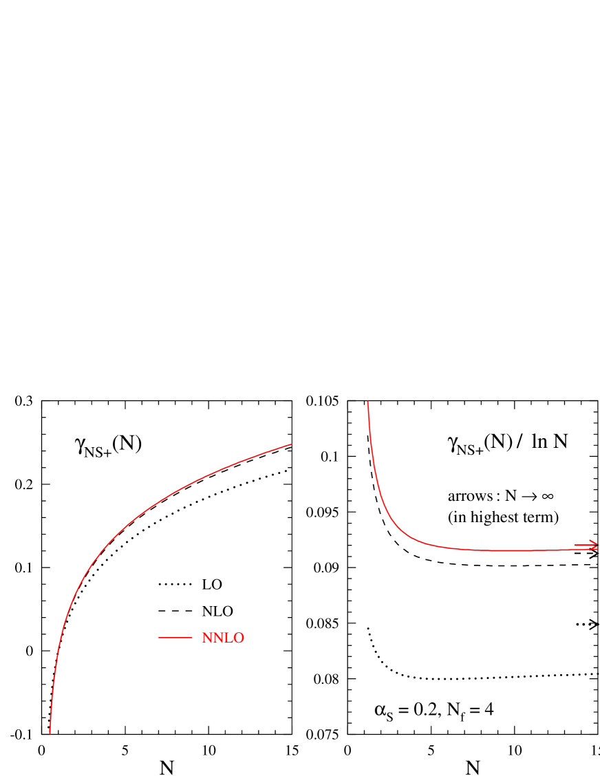
Figure 1: The perturbative expansion of the anomalous dimension $\gamma_{\,\rm ns}^{\,+}(N)$ for four flavours at $\alpha_{\rm s}=0.2$. In the right part the leading $N$-dependence for large $N$ has been divided out, and the corresponding asymptotic limits are indicated as discussed in the text.

The results (3.4), (3.5) and (3.7) for $\gamma_{\rm ns}^{\,+}(N)$ are assembled in Fig. 1 for four active flavours and a typical value $\alpha_{\rm s}=0.2$ for the strong coupling constant (recall that the terms up to order $\alpha_{\rm s}^{\,n+1}$ are included at N${}^{\,\rm n}$LO). Numerically, the colour factors take the values ${C_{F}}=4/3,{C_{A}}=3$ and ${d^{abc}d_{abc}}/n_{c}=40/9$. Note that the latter normalization is different from that employed in Ref. [58].

The NNLO corrections are rather small under these circumstances, amounting to less than 2% for $N\geq 2$. At large $N$ the anomalous dimensions behave as

$$\gamma_{\,\rm ns}^{\,(n)\pm,\rm v}(N)\>=\>\>A_{n}(\ln N+\gamma_{e})-B_{n}-C_{n}\>\frac{\ln N}{N}+{\cal O}\left(\frac{1}{N}\right)$$ (3.10)

where $\gamma_{e}$ is the Euler-Mascheroni constant and the coefficients are specified in the next paragraph. Thus $\tilde{\gamma}_{\,\rm ns}^{\,+}=\gamma_{\,\rm ns}^{\,+}/\ln N$, also shown in Fig. 1, approaches a constant for $N\rightarrow\infty$. The asymptotic results are indicated by replacing $\tilde{\gamma}_{\,\rm ns}^{\,(n)+}(N=15)$ by $\tilde{\gamma}_{\,\rm ns}^{\,(n)+}(N\rightarrow\infty)$ for the respective highest term included in the curves (e.g., for $n=2$ at NNLO). Obviously the approach to the asymptotic limit is very slow. Yet the results at $N\rightarrow\infty$, which can be derived much easier than the full $N$-dependence [73], do provide a reasonable first estimate of the corrections.

The leading large-$N$ coefficients $A_{n}$, which are also relevant for the soft-gluon (threshold) resummation [34, 35, 36, 37], are given by

$$A_{1} = 4\,C_{F}$$

$$A_{2} = 8\,C_{F}\left[\left(\frac{67}{18}-\zeta_{2}\right)C_{A}-\frac{5}{9}\,{n_{\!f}}\right]$$

$$A_{3} = 16\,C_{F}C_{A}^{\,2}\,\left(\frac{245}{24}-\frac{67}{9}\>{\zeta_{2}}+\frac{11}{6}\>{\zeta_{3}}+\frac{11}{5}\>{\zeta_{2}}^{\!\!2}\right)\>+\>16\,C_{F}^{\,2}{n_{\!f}}\,\left(-\frac{55}{24}+2\>{\zeta_{3}}\right)$$ (3.11)

$$\mbox{}+\>16\,C_{F}C_{A}{n_{\!f}}\,\left(-\frac{209}{108}+\frac{10}{9}\>{\zeta_{2}}-\frac{7}{3}\>{\zeta_{3}}\right)\>+\>16\,C_{F}{n^{\,2}_{\!f}}\left(-\frac{1}{27}\,\right)\>\>.$$

The ${n_{\!f}}$-independent contribution to the three-loop coefficient $A_{3}$ is also a new result of the present article. Inserting the numerical values of the $\zeta$-function and the QCD colour factors it reads $A_{3}|_{{n_{\!f}}=0}\cong 1174.898$, in agreement with the previous numerical estimate of Ref. [37]. The constants $B_{n}$ can be read off directly from the terms with $\delta(1-x)$ in Eqs. (4.5), (4) and (4.9) below. Surprisingly, the coefficients $C_{n}$ in Eq. (3.10), which are also best determined using those $x$-space results, turn out to be related to the $A_{n}$ by

$$C_{1}\>\>=\>\>0\>\>,\quad C_{2}\>\>=\>\>4\,C_{F}\>A_{1}\>\>,\quad C_{3}\>\>=\>\>8\,C_{F}\>A_{2}\>\>.$$ (3.12)

Especially the relation for $C_{3}$ is very suggestive and seems to call for a structural explanation.

4 Results in x-space

The splitting functions $P_{\,\rm ns}^{\,(n)\pm,s}(x)$ are obtained from the $N$-space results of the previous section by an inverse Mellin transformation, which expresses these functions in terms of harmonic polylogarithms [62, 63, 64]. The inverse Mellin transformation exploits an isomorphism between the set of harmonic sums for even or odd $N$ and the set of harmonic polylogarithms. Hence it can be performed by a completely algebraic procedure [45, 64], based on the fact that harmonic sums occur as coefficients of the Taylor expansion of harmonic polylogarithms.

Our notation for the harmonic polylogarithms $H_{m_{1},...,m_{w}}(x)$, $m_{j}=0,\pm 1$ follows Ref. [64] to which the reader is referred for a detailed discussion. The lowest-weight ($w=1$) functions $H_{m}(x)$ are given by

$$H_{0}(x)\>=\>\ln x\>\>,\quad\quad H_{\pm 1}(x)\>=\>\mp\,\ln(1\mp x)\>\>.$$ (4.1)

The higher-weight ($w\geq 2$) functions are recursively defined as

$$H_{m_{1},...,m_{w}}(x)\>=\>\left\{\begin{array}[]{cl}\displaystyle{\frac{1}{w!}\,\ln^{w}x\>\>,}&\quad{\rm if}\>\>\>m_{1},...,m_{w}=0,\ldots,0\\[8.61108pt] \displaystyle{\int_{0}^{x}\!dz\>f_{m_{1}}(z)\,H_{m_{2},...,m_{w}}(z)\>\>,}&\quad{\rm else}\end{array}\right.$$ (4.2)

with

$$f_{0}(x)\>=\>\frac{1}{x}\>\>,\quad\quad f_{\pm 1}(x)\>=\>\frac{1}{1\mp x}\>\>.$$ (4.3)

A useful short-hand notation is

$$H_{{\footnotesize\underbrace{0,\ldots,0}_{\scriptstyle m}},\,\pm 1,\,{\footnotesize\underbrace{0,\ldots,0}_{\scriptstyle n}},\,\pm 1,\,\ldots}(x)\>=\>H_{\pm(m+1),\,\pm(n+1),\,\ldots}(x)\>\>.$$ (4.4)

For $w\leq 3$ the harmonic polylogarithms can be expressed in terms of standard polylogarithms; a complete list can be found in appendix A of Ref. [45]. All harmonic polylogarithms of weight $w=4$ in this article can be expressed in terms of standard polylogarithms, Nielsen functions [74] or, by means of the defining relation (4.2), as one-dimensional integrals over these functions. A Fortran program for the functions up to weight $w=4$ has been provided in Ref. [75].

For completeness we recall the one- and two-loop non-singlet splitting functions [3, 8]

$$P^{\,(0)}_{\,\rm ns}(x) \!=\! {{C_{F}}}\*\big{(}\,2\*p_{\rm{qq}}(x)+3\*\delta(1-x)\,\big{)}$$ (4.5)

and

$$P^{\,(1)+}_{\,\rm ns}(x)\>\>=\>4\,\*{{C_{A}}\*{C_{F}}}\*\bigg{(}p_{\rm{qq}}(x)\*\bigg{[}{67\over 18}-{\zeta_{2}}+{11\over 6}\*{\rm{H}}_{0}+{\rm{H}}_{0,0}\bigg{]}+p_{\rm{qq}}(-x)\*\bigg{[}{\zeta_{2}}+2\*{\rm{H}}_{-1,0}-{\rm{H}}_{0,0}\bigg{]}$$

$$\mbox{}\quad+{14\over 3}\*(1-x)+\delta(1-x)\*\bigg{[}{17\over 24}+{11\over 3}\*{\zeta_{2}}-3\*{\zeta_{3}}\bigg{]}\bigg{)}-4\,\*{{C_{F}}\*{n_{\!f}}}\*\bigg{(}p_{\rm{qq}}(x)\*\bigg{[}{5\over 9}+{1\over 3}\*{\rm{H}}_{0}\bigg{]}+{2\over 3}\*(1-x)$$

$$\mbox{}\quad+\delta(1-x)\*\bigg{[}{1\over 12}+{2\over 3}\*{\zeta_{2}}\bigg{]}\bigg{)}+4\,\*{{C_{F}}^{2}}\*\bigg{(}2\*p_{\rm{qq}}(x)\*\bigg{[}{\rm{H}}_{1,0}-{3\over 4}\*{\rm{H}}_{0}+{\rm{H}}_{2}\bigg{]}-2\*p_{\rm{qq}}(-x)\*\bigg{[}{\zeta_{2}}+2\*{\rm{H}}_{-1,0}\quad$$

$$\mbox{}\quad-{\rm{H}}_{0,0}\bigg{]}-(1-x)\*\bigg{[}1-{3\over 2}\*{\rm{H}}_{0}\bigg{]}-{\rm{H}}_{0}-(1+x)\*{\rm{H}}_{0,0}+\delta(1-x)\*\bigg{[}{3\over 8}-3\*{\zeta_{2}}+6\*{\zeta_{3}}\bigg{]}\bigg{)}\>\>,$$ (4.6)

$$P^{\,(1)-}_{\,\rm ns}(x)\>\>=\>\>P^{\,(1)+}_{\,\rm ns}(x)+16\,\*{{C_{F}}\*\bigg{(}{C_{F}}-{{C_{A}}\over 2}\bigg{)}}\*\bigg{(}p_{\rm{qq}}(-x)\*\bigg{[}{\zeta_{2}}+2\*{\rm{H}}_{-1,0}-{\rm{H}}_{0,0}\bigg{]}-2\*(1-x)$$

$$\mbox{}\quad-(1+x)\*{\rm{H}}_{0}\bigg{)}\>\>.$$ (4.7)

Here and in Eqs. (4.9) – (4.11) we suppress the argument $x$ of the polylogarithms and use

$$p_{\rm{qq}}(x)\>=\>2\,(1-x)^{-1}-1-x\>\>.$$ (4.8)

All divergences for $x\to 1$ are understood in the sense of $+$-distributions.

The three-loop splitting function for the evolution of the ‘plus’ combinations of quark densities in Eq. (2.2), corresponding to the anomalous dimension (3.8) reads

$$P^{\,(2)+}_{\,\rm ns}(x)\>\>=\>\>16\,\*{{C_{A}}\*{C_{F}}\*{n_{\!f}}}\*\bigg{(}{1\over 6}\*p_{\rm{qq}}(x)\*\bigg{[}{10\over 3}\*{\zeta_{2}}-{209\over 36}-9\*{\zeta_{3}}-{167\over 18}\*{\rm{H}}_{0}+2\*{\rm{H}}_{0}\*{\zeta_{2}}-7\*{\rm{H}}_{0,0}-2\*{\rm{H}}_{0,0,0}$$

$$\mbox{}+3\*{\rm{H}}_{1,0,0}-{\rm{H}}_{3}\bigg{]}+{1\over 3}\*p_{\rm{qq}}(-x)\*\bigg{[}{3\over 2}\*{\zeta_{3}}-{5\over 3}\*{\zeta_{2}}-{\rm{H}}_{-2,0}-2\*{\rm{H}}_{-1}\*{\zeta_{2}}-{10\over 3}\*{\rm{H}}_{-1,0}-{\rm{H}}_{-1,0,0}$$

$$\mbox{}+2\*{\rm{H}}_{-1,2}+{1\over 2}\*{\rm{H}}_{0}\*{\zeta_{2}}+{5\over 3}\*{\rm{H}}_{0,0}+{\rm{H}}_{0,0,0}-{\rm{H}}_{3}\bigg{]}+(1-x)\*\bigg{[}{1\over 6}\*{\zeta_{2}}-{257\over 54}-{43\over 18}\*{\rm{H}}_{0}-{1\over 6}\*{\rm{H}}_{0,0}-{\rm{H}}_{1}\bigg{]}$$

$$\mbox{}-(1+x)\*\bigg{[}{2\over 3}\*{\rm{H}}_{-1,0}+{1\over 2}\*{\rm{H}}_{2}\bigg{]}+{1\over 3}\*{\zeta_{2}}+{\rm{H}}_{0}+{1\over 6}\*{\rm{H}}_{0,0}+\delta(1-x)\*\bigg{[}{5\over 4}-{167\over 54}\*{\zeta_{2}}+{1\over 20}\*{\zeta_{2}}^{2}+{25\over 18}\*{\zeta_{3}}\bigg{]}\bigg{)}$$

$$\mbox{}+16\,\*{{C_{A}}\*{C_{F}}^{2}}\*\bigg{(}p_{\rm{qq}}(x)\*\bigg{[}{5\over 6}\*{\zeta_{3}}-{69\over 20}\*{\zeta_{2}}^{2}-{\rm{H}}_{-3,0}-3\*{\rm{H}}_{-2}\*{\zeta_{2}}-14\*{\rm{H}}_{-2,-1,0}+3\*{\rm{H}}_{-2,0}+5\*{\rm{H}}_{-2,0,0}$$

$$\mbox{}-4\*{\rm{H}}_{-2,2}-{151\over 48}\*{\rm{H}}_{0}+{41\over 12}\*{\rm{H}}_{0}\*{\zeta_{2}}-{17\over 2}\*{\rm{H}}_{0}\*{\zeta_{3}}-{13\over 4}\*{\rm{H}}_{0,0}-4\*{\rm{H}}_{0,0}\*{\zeta_{2}}-{23\over 12}\*{\rm{H}}_{0,0,0}+5\*{\rm{H}}_{0,0,0,0}+{2\over 3}\*{\rm{H}}_{3}$$

$$\mbox{}-24\*{\rm{H}}_{1}\*{\zeta_{3}}-16\*{\rm{H}}_{1,-2,0}+{67\over 9}\*{\rm{H}}_{1,0}-2\*{\rm{H}}_{1,0}\*{\zeta_{2}}+{31\over 3}\*{\rm{H}}_{1,0,0}+11\*{\rm{H}}_{1,0,0,0}+8\*{\rm{H}}_{1,1,0,0}-8\*{\rm{H}}_{1,3}+{\rm{H}}_{4}$$

$$\mbox{}+{67\over 9}\*{\rm{H}}_{2}-2\*{\rm{H}}_{2}\*{\zeta_{2}}+{11\over 3}\*{\rm{H}}_{2,0}+5\*{\rm{H}}_{2,0,0}+{\rm{H}}_{3,0}\bigg{]}+p_{\rm{qq}}(-x)\*\bigg{[}{1\over 4}\*{\zeta_{2}}^{2}-{67\over 9}\*{\zeta_{2}}+{31\over 4}\*{\zeta_{3}}+5\*{\rm{H}}_{-3,0}$$

$$\mbox{}-32\*{\rm{H}}_{-2}\*{\zeta_{2}}-4\*{\rm{H}}_{-2,-1,0}-{31\over 6}\*{\rm{H}}_{-2,0}+21\*{\rm{H}}_{-2,0,0}+30\*{\rm{H}}_{-2,2}-{31\over 3}\*{\rm{H}}_{-1}\*{\zeta_{2}}-42\*{\rm{H}}_{-1}\*{\zeta_{3}}+{9\over 4}\*{\rm{H}}_{0}$$

$$\mbox{}-4\*{\rm{H}}_{-1,-2,0}+56\*{\rm{H}}_{-1,-1}\*{\zeta_{2}}-36\*{\rm{H}}_{-1,-1,0,0}-56\*{\rm{H}}_{-1,-1,2}-{134\over 9}\*{\rm{H}}_{-1,0}-42\*{\rm{H}}_{-1,0}\*{\zeta_{2}}-{\rm{H}}_{3,0}$$

$$\mbox{}+32\*{\rm{H}}_{-1,3}-{31\over 6}\*{\rm{H}}_{-1,0,0}+17\*{\rm{H}}_{-1,0,0,0}+{31\over 3}\*{\rm{H}}_{-1,2}+2\*{\rm{H}}_{-1,2,0}+{13\over 12}\*{\rm{H}}_{0}\*{\zeta_{2}}+{29\over 2}\*{\rm{H}}_{0}\*{\zeta_{3}}+{67\over 9}\*{\rm{H}}_{0,0}$$

$$\mbox{}+13\*{\rm{H}}_{0,0}\*{\zeta_{2}}+{89\over 12}\*{\rm{H}}_{0,0,0}-5\*{\rm{H}}_{0,0,0,0}-7\*{\rm{H}}_{2}\*{\zeta_{2}}-{31\over 6}\*{\rm{H}}_{3}-10\*{\rm{H}}_{4}\bigg{]}+(1-x)\*\bigg{[}{133\over 36}+4\*{\rm{H}}_{0,0,0,0}$$

$$\mbox{}-{167\over 4}\*{\zeta_{3}}-2\*{\rm{H}}_{0}\*{\zeta_{3}}-2\*{\rm{H}}_{-3,0}+{\rm{H}}_{-2}\*{\zeta_{2}}+2\*{\rm{H}}_{-2,-1,0}-3\*{\rm{H}}_{-2,0,0}+{77\over 4}\*{\rm{H}}_{0,0,0}-{209\over 6}\*{\rm{H}}_{1}-7\*{\rm{H}}_{1}\*{\zeta_{2}}$$

$$\mbox{}+4\*{\rm{H}}_{1,0,0}+{14\over 3}\*{\rm{H}}_{1,0}\bigg{]}+(1+x)\*\bigg{[}{43\over 2}\*{\zeta_{2}}-3\*{\zeta_{2}}^{2}+{25\over 2}\*{\rm{H}}_{-2,0}-31\*{\rm{H}}_{-1}\*{\zeta_{2}}-14\*{\rm{H}}_{-1,-1,0}-{13\over 3}\*{\rm{H}}_{-1,0}$$

$$\mbox{}+24\*{\rm{H}}_{-1,2}+23\*{\rm{H}}_{-1,0,0}+{55\over 2}\*{\rm{H}}_{0}\*{\zeta_{2}}+5\*{\rm{H}}_{0,0}\*{\zeta_{2}}+{1457\over 48}\*{\rm{H}}_{0}-{1025\over 36}\*{\rm{H}}_{0,0}-{155\over 6}\*{\rm{H}}_{2}+{\rm{H}}_{2}\*{\zeta_{2}}-15\*{\rm{H}}_{3}$$

$$\mbox{}+2\*{\rm{H}}_{2,0,0}-3\*{\rm{H}}_{4}\bigg{]}-5\*{\zeta_{2}}-{1\over 2}\*{\zeta_{2}}^{2}+50\*{\zeta_{3}}-2\*{\rm{H}}_{-3,0}-7\*{\rm{H}}_{-2,0}-{\rm{H}}_{0}\*{\zeta_{3}}-{37\over 2}\*{\rm{H}}_{0}\*{\zeta_{2}}-{242\over 9}\*{\rm{H}}_{0}$$

$$\mbox{}-2\*{\rm{H}}_{0,0}\*{\zeta_{2}}+{185\over 6}\*{\rm{H}}_{0,0}-22\*{\rm{H}}_{0,0,0}-4\*{\rm{H}}_{0,0,0,0}+{28\over 3}\*{\rm{H}}_{2}+6\*{\rm{H}}_{3}+\delta(1-x)\*\bigg{[}{151\over 64}+{\zeta_{2}}\*{\zeta_{3}}-{205\over 24}\*{\zeta_{2}}$$

$$\mbox{}-{247\over 60}\*{\zeta_{2}}^{2}+{211\over 12}\*{\zeta_{3}}+{15\over 2}\*{\zeta_{5}}\bigg{]}\bigg{)}+16\,\*{{C_{A}}^{2}\*{C_{F}}}\*\bigg{(}p_{\rm{qq}}(x)\*\bigg{[}{245\over 48}-{67\over 18}\*{\zeta_{2}}+{12\over 5}\*{\zeta_{2}}^{2}+{1\over 2}\*{\zeta_{3}}+{1043\over 216}\*{\rm{H}}_{0}$$

$$\mbox{}+{\rm{H}}_{-3,0}+4\*{\rm{H}}_{-2,-1,0}-{3\over 2}\*{\rm{H}}_{-2,0}-{\rm{H}}_{-2,0,0}+2\*{\rm{H}}_{-2,2}-{31\over 12}\*{\rm{H}}_{0}\*{\zeta_{2}}+4\*{\rm{H}}_{0}\*{\zeta_{3}}+{389\over 72}\*{\rm{H}}_{0,0}-2\*{\rm{H}}_{2,0,0}$$

$$\mbox{}-{\rm{H}}_{0,0,0,0}+9\*{\rm{H}}_{1}\*{\zeta_{3}}+6\*{\rm{H}}_{1,-2,0}-{\rm{H}}_{1,0}\*{\zeta_{2}}-{11\over 4}\*{\rm{H}}_{1,0,0}-3\*{\rm{H}}_{1,0,0,0}-4\*{\rm{H}}_{1,1,0,0}+4\*{\rm{H}}_{1,3}+{31\over 12}\*{\rm{H}}_{0,0,0}$$

$$\mbox{}+{11\over 12}\*{\rm{H}}_{3}+{\rm{H}}_{4}\bigg{]}+p_{\rm{qq}}(-x)\*\bigg{[}{67\over 18}\*{\zeta_{2}}-{\zeta_{2}}^{2}-{11\over 4}\*{\zeta_{3}}-{\rm{H}}_{-3,0}+8\*{\rm{H}}_{-2}\*{\zeta_{2}}+{11\over 6}\*{\rm{H}}_{-2,0}-4\*{\rm{H}}_{-2,0,0}$$

$$\mbox{}-3\*{\rm{H}}_{-1,0,0,0}+{11\over 3}\*{\rm{H}}_{-1}\*{\zeta_{2}}+12\*{\rm{H}}_{-1}\*{\zeta_{3}}-16\*{\rm{H}}_{-1,-1}\*{\zeta_{2}}+8\*{\rm{H}}_{-1,-1,0,0}+16\*{\rm{H}}_{-1,-1,2}+{67\over 9}\*{\rm{H}}_{-1,0}$$

$$\mbox{}-8\*{\rm{H}}_{-2,2}+11\*{\rm{H}}_{-1,0}\*{\zeta_{2}}+{11\over 6}\*{\rm{H}}_{-1,0,0}-{11\over 3}\*{\rm{H}}_{-1,2}-8\*{\rm{H}}_{-1,3}-{3\over 4}\*{\rm{H}}_{0}-{1\over 6}\*{\rm{H}}_{0}\*{\zeta_{2}}-4\*{\rm{H}}_{0}\*{\zeta_{3}}-{67\over 18}\*{\rm{H}}_{0,0}$$

$$\mbox{}-3\*{\rm{H}}_{0,0}\*{\zeta_{2}}-{31\over 12}\*{\rm{H}}_{0,0,0}+{\rm{H}}_{0,0,0,0}+2\*{\rm{H}}_{2}\*{\zeta_{2}}+{11\over 6}\*{\rm{H}}_{3}+2\*{\rm{H}}_{4}\bigg{]}+(1-x)\*\bigg{[}{1883\over 108}-{1\over 2}\*{\rm{H}}_{0,0,0,0}+11\*{\rm{H}}_{1}$$

$$\mbox{}-{\rm{H}}_{-2,-1,0}+{1\over 2}\*{\rm{H}}_{-3,0}-{1\over 2}\*{\rm{H}}_{-2}\*{\zeta_{2}}+{1\over 2}\*{\rm{H}}_{-2,0,0}+{523\over 36}\*{\rm{H}}_{0}+{\rm{H}}_{0}\*{\zeta_{3}}-{13\over 3}\*{\rm{H}}_{0,0}-{5\over 2}\*{\rm{H}}_{0,0,0}+2\*{\rm{H}}_{1}\*{\zeta_{2}}$$

$$\mbox{}-2\*{\rm{H}}_{1,0,0}\bigg{]}+(1+x)\*\bigg{[}8\*{\rm{H}}_{-1}\*{\zeta_{2}}+4\*{\rm{H}}_{-1,-1,0}+{8\over 3}\*{\rm{H}}_{-1,0}-5\*{\rm{H}}_{-1,0,0}-6\*{\rm{H}}_{-1,2}-{13\over 3}\*{\zeta_{2}}+{3\over 8}\*{\zeta_{2}}^{2}$$

$$\mbox{}-{43\over 4}\*{\zeta_{3}}-{5\over 2}\*{\rm{H}}_{-2,0}-{11\over 2}\*{\rm{H}}_{0}\*{\zeta_{2}}-{1\over 2}\*{\rm{H}}_{2}\*{\zeta_{2}}-{5\over 4}\*{\rm{H}}_{0,0}\*{\zeta_{2}}+7\*{\rm{H}}_{2}-{1\over 4}\*{\rm{H}}_{2,0,0}+3\*{\rm{H}}_{3}+{3\over 4}\*{\rm{H}}_{4}\bigg{]}+{1\over 2}\*{\rm{H}}_{0,0}\*{\zeta_{2}}$$

$$\mbox{}+{1\over 4}\*{\zeta_{2}}^{2}-{8\over 3}\*{\zeta_{2}}+{17\over 2}\*{\zeta_{3}}+{\rm{H}}_{-2,0}-{19\over 2}\*{\rm{H}}_{0}+{5\over 2}\*{\rm{H}}_{0}\*{\zeta_{2}}-{\rm{H}}_{0}\*{\zeta_{3}}+{13\over 3}\*{\rm{H}}_{0,0}+{5\over 2}\*{\rm{H}}_{0,0,0}+{1\over 2}\*{\rm{H}}_{0,0,0,0}$$

$$\mbox{}-\delta(1-x)\*\bigg{[}{1657\over 576}-{281\over 27}\*{\zeta_{2}}+{1\over 8}\*{\zeta_{2}}^{2}+{97\over 9}\*{\zeta_{3}}-{5\over 2}\*{\zeta_{5}}\bigg{]}\bigg{)}+16\,\*{{C_{F}}\*{n^{\,2}_{\!f}}}\*\bigg{(}{1\over 18}\*p_{\rm{qq}}(x)\*\bigg{[}{\rm{H}}_{0,0}-{1\over 3}+{5\over 3}\*{\rm{H}}_{0}\bigg{]}$$

$$\mbox{}+(1-x)\*\bigg{[}{13\over 54}+{1\over 9}\*{\rm{H}}_{0}\bigg{]}-\delta(1-x)\*\bigg{[}{17\over 144}-{5\over 27}\*{\zeta_{2}}+{1\over 9}\*{\zeta_{3}}\bigg{]}\bigg{)}+16\,\*{{C_{F}}^{2}\*{n_{\!f}}}\*\bigg{(}{1\over 3}\*p_{\rm{qq}}(x)\*\bigg{[}5\*{\zeta_{3}}-4\*{\rm{H}}_{1,0,0}$$

$$\mbox{}-{55\over 16}+{5\over 8}\*{\rm{H}}_{0}+{\rm{H}}_{0}\*{\zeta_{2}}+{3\over 2}\*{\rm{H}}_{0,0}-{\rm{H}}_{0,0,0}-{10\over 3}\*{\rm{H}}_{1,0}-{10\over 3}\*{\rm{H}}_{2}-2\*{\rm{H}}_{2,0}-2\*{\rm{H}}_{3}\bigg{]}+{2\over 3}\*p_{\rm{qq}}(-x)\*\bigg{[}{5\over 3}\*{\zeta_{2}}$$

$$\mbox{}-{3\over 2}\*{\zeta_{3}}+{\rm{H}}_{-2,0}+2\*{\rm{H}}_{-1}\*{\zeta_{2}}+{10\over 3}\*{\rm{H}}_{-1,0}+{\rm{H}}_{-1,0,0}-2\*{\rm{H}}_{-1,2}-{1\over 2}\*{\rm{H}}_{0}\*{\zeta_{2}}-{5\over 3}\*{\rm{H}}_{0,0}-{\rm{H}}_{0,0,0}+{\rm{H}}_{3}\bigg{]}$$

$$\mbox{}-(1-x)\*\bigg{[}{10\over 9}+{19\over 18}\*{\rm{H}}_{0,0}-{4\over 3}\*{\rm{H}}_{1}+{2\over 3}\*{\rm{H}}_{1,0}+{4\over 3}\*{\rm{H}}_{2}\bigg{]}+(1+x)\*\bigg{[}{4\over 3}\*{\rm{H}}_{-1,0}-{25\over 24}\*{\rm{H}}_{0}+{1\over 2}\*{\rm{H}}_{0,0,0}\bigg{]}+{2\over 9}\*{\rm{H}}_{0}$$

$$\mbox{}+{7\over 9}\*{\rm{H}}_{0,0}+{4\over 3}\*{\rm{H}}_{2}-\delta(1-x)\*\bigg{[}{23\over 16}-{5\over 12}\*{\zeta_{2}}-{29\over 30}\*{\zeta_{2}}^{2}+{17\over 6}\*{\zeta_{3}}\bigg{]}\bigg{)}+16\,\*{{C_{F}}^{3}}\*\bigg{(}p_{\rm{qq}}(x)\*\bigg{[}{9\over 10}\*{\zeta_{2}}^{2}-2\*{\rm{H}}_{-3,0}$$

$$\mbox{}+6\*{\rm{H}}_{-2}\*{\zeta_{2}}+12\*{\rm{H}}_{-2,-1,0}-6\*{\rm{H}}_{-2,0,0}-{3\over 16}\*{\rm{H}}_{0}-{3\over 2}\*{\rm{H}}_{0}\*{\zeta_{2}}+{\rm{H}}_{0}\*{\zeta_{3}}+{13\over 8}\*{\rm{H}}_{0,0}-2\*{\rm{H}}_{0,0,0,0}+8\*{\rm{H}}_{1,3}$$

$$\mbox{}+12\*{\rm{H}}_{1}\*{\zeta_{3}}+8\*{\rm{H}}_{1,-2,0}-6\*{\rm{H}}_{1,0,0}-4\*{\rm{H}}_{1,0,0,0}+4\*{\rm{H}}_{1,2,0}-3\*{\rm{H}}_{2,0}+2\*{\rm{H}}_{2,0,0}+4\*{\rm{H}}_{2,1,0}+4\*{\rm{H}}_{2,2}$$

$$\mbox{}+4\*{\rm{H}}_{3,0}+4\*{\rm{H}}_{3,1}+2\*{\rm{H}}_{4}\bigg{]}+p_{\rm{qq}}(-x)\*\bigg{[}{7\over 2}\*{\zeta_{2}}^{2}-{9\over 2}\*{\zeta_{3}}-6\*{\rm{H}}_{-3,0}+32\*{\rm{H}}_{-2}\*{\zeta_{2}}+8\*{\rm{H}}_{-2,-1,0}+3\*{\rm{H}}_{-2,0}$$

$$\mbox{}-26\*{\rm{H}}_{-2,0,0}-28\*{\rm{H}}_{-2,2}+6\*{\rm{H}}_{-1}\*{\zeta_{2}}+36\*{\rm{H}}_{-1}\*{\zeta_{3}}+8\*{\rm{H}}_{-1,-2,0}-48\*{\rm{H}}_{-1,-1}\*{\zeta_{2}}+40\*{\rm{H}}_{-1,-1,0,0}$$

$$\mbox{}+48\*{\rm{H}}_{-1,-1,2}+40\*{\rm{H}}_{-1,0}\*{\zeta_{2}}+3\*{\rm{H}}_{-1,0,0}-22\*{\rm{H}}_{-1,0,0,0}-6\*{\rm{H}}_{-1,2}-4\*{\rm{H}}_{-1,2,0}-32\*{\rm{H}}_{-1,3}-{3\over 2}\*{\rm{H}}_{0}$$

$$\mbox{}-{3\over 2}\*{\rm{H}}_{0}\*{\zeta_{2}}-13\*{\rm{H}}_{0}\*{\zeta_{3}}-14\*{\rm{H}}_{0,0}\*{\zeta_{2}}-{9\over 2}\*{\rm{H}}_{0,0,0}+6\*{\rm{H}}_{0,0,0,0}+6\*{\rm{H}}_{2}\*{\zeta_{2}}+3\*{\rm{H}}_{3}+2\*{\rm{H}}_{3,0}+12\*{\rm{H}}_{4}\bigg{]}$$

$$\mbox{}+(1-x)\*\bigg{[}2\*{\rm{H}}_{-3,0}-{31\over 8}+4\*{\rm{H}}_{-2,0,0}+{\rm{H}}_{0,0}\*{\zeta_{2}}-3\*{\rm{H}}_{0,0,0,0}+35\*{\rm{H}}_{1}+6\*{\rm{H}}_{1}\*{\zeta_{2}}-{\rm{H}}_{1,0}+{5\over 2}\*{\rm{H}}_{2,0}\bigg{]}$$

$$\mbox{}+(1+x)\*\bigg{[}{37\over 10}\*{\zeta_{2}}^{2}-{93\over 4}\*{\zeta_{2}}-{81\over 2}\*{\zeta_{3}}-15\*{\rm{H}}_{-2,0}+30\*{\rm{H}}_{-1}\*{\zeta_{2}}+12\*{\rm{H}}_{-1,-1,0}-2\*{\rm{H}}_{-1,0}-26\*{\rm{H}}_{-1,0,0}$$

$$\mbox{}-24\*{\rm{H}}_{-1,2}-{539\over 16}\*{\rm{H}}_{0}-28\*{\rm{H}}_{0}\*{\zeta_{2}}+{191\over 8}\*{\rm{H}}_{0,0}+20\*{\rm{H}}_{0,0,0}+{85\over 4}\*{\rm{H}}_{2}-3\*{\rm{H}}_{2,0,0}-2\*{\rm{H}}_{3,0}+13\*{\rm{H}}_{3}$$

$$\mbox{}-{\rm{H}}_{4}\bigg{]}+4\*{\zeta_{2}}+33\*{\zeta_{3}}+4\*{\rm{H}}_{-3,0}+10\*{\rm{H}}_{-2,0}+{67\over 2}\*{\rm{H}}_{0}+6\*{\rm{H}}_{0}\*{\zeta_{3}}+19\*{\rm{H}}_{0}\*{\zeta_{2}}-25\*{\rm{H}}_{0,0}-17\*{\rm{H}}_{0,0,0}$$

$$\mbox{}-2\*{\rm{H}}_{2}-{\rm{H}}_{2,0}-4\*{\rm{H}}_{3}+\delta(1-x)\*\bigg{[}{29\over 32}-2\*{\zeta_{2}}\*{\zeta_{3}}+{9\over 8}\*{\zeta_{2}}+{18\over 5}\*{\zeta_{2}}^{2}+{17\over 4}\*{\zeta_{3}}-15\*{\zeta_{5}}\bigg{]}\bigg{)}\>\>.$$ (4.9)

The $x$-space counterpart of Eq. (3.8) for the evolution of the ‘minus’ combinations (2.2) is given by

$$P^{\,(2)-}_{\,\rm ns}(x)\>\>=\>\>P^{\,(2)+}_{\,\rm ns}(x)+16\,\*{{C_{A}}\*{C_{F}}\*\bigg{(}{C_{F}}-{{C_{A}}\over 2}\bigg{)}}\*\bigg{(}p_{\rm{qq}}(-x)\*\bigg{[}{134\over 9}\*{\zeta_{2}}-4\*{\zeta_{2}}^{2}-11\*{\zeta_{3}}-4\*{\rm{H}}_{-3,0}$$

$$\mbox{}+32\*{\rm{H}}_{-2}\*{\zeta_{2}}+{22\over 3}\*{\rm{H}}_{-2,0}-16\*{\rm{H}}_{-2,0,0}-32\*{\rm{H}}_{-2,2}+{44\over 3}\*{\rm{H}}_{-1}\*{\zeta_{2}}+48\*{\rm{H}}_{-1}\*{\zeta_{3}}-64\*{\rm{H}}_{-1,-1}\*{\zeta_{2}}$$

$$\mbox{}+32\*{\rm{H}}_{-1,-1,0,0}+64\*{\rm{H}}_{-1,-1,2}+{268\over 9}\*{\rm{H}}_{-1,0}+44\*{\rm{H}}_{-1,0}\*{\zeta_{2}}+{22\over 3}\*{\rm{H}}_{-1,0,0}-12\*{\rm{H}}_{-1,0,0,0}-{44\over 3}\*{\rm{H}}_{-1,2}$$

$$\mbox{}-32\*{\rm{H}}_{-1,3}-3\*{\rm{H}}_{0}-{2\over 3}\*{\rm{H}}_{0}\*{\zeta_{2}}-16\*{\rm{H}}_{0}\*{\zeta_{3}}-{134\over 9}\*{\rm{H}}_{0,0}-12\*{\rm{H}}_{0,0}\*{\zeta_{2}}-{31\over 3}\*{\rm{H}}_{0,0,0}+4\*{\rm{H}}_{0,0,0,0}+8\*{\rm{H}}_{2}\*{\zeta_{2}}$$

$$\mbox{}+{22\over 3}\*{\rm{H}}_{3}+8\*{\rm{H}}_{4}\bigg{]}+(1-x)\*\bigg{[}{367\over 18}+{1\over 2}\*{\zeta_{2}}^{2}+2\*{\rm{H}}_{-3,0}-2\*{\rm{H}}_{-2}\*{\zeta_{2}}-4\*{\rm{H}}_{-2,-1,0}-10\*{\rm{H}}_{-2,0}-2\*{\rm{H}}_{0,0}$$

$$\mbox{}+2\*{\rm{H}}_{-2,0,0}+2\*{\rm{H}}_{0}\*{\zeta_{3}}+{\rm{H}}_{0,0}\*{\zeta_{2}}-{\rm{H}}_{0,0,0,0}+8\*{\rm{H}}_{1}\*{\zeta_{2}}+{140\over 3}\*{\rm{H}}_{1}\bigg{]}+(1+x)\*\bigg{[}32\*{\rm{H}}_{-1}\*{\zeta_{2}}-18\*{\zeta_{2}}$$

$$\mbox{}-23\*{\zeta_{3}}+{26\over 3}\*{\rm{H}}_{-1,0}-16\*{\rm{H}}_{-1,0,0}-32\*{\rm{H}}_{-1,2}-{481\over 18}\*{\rm{H}}_{0}-29\*{\rm{H}}_{0}\*{\zeta_{2}}+5\*{\rm{H}}_{0,0,0}+24\*{\rm{H}}_{3}+{70\over 3}\*{\rm{H}}_{2}\bigg{]}$$

$$\mbox{}-2\*{\zeta_{2}}-2\*{\zeta_{3}}+32\*{\rm{H}}_{0}+14\*{\rm{H}}_{0}\*{\zeta_{2}}+2\*{\rm{H}}_{0,0,0}-16\*{\rm{H}}_{3}\bigg{)}+16\,\*{{C_{F}}\*{n_{\!f}}\*\bigg{(}{C_{F}}-{{C_{A}}\over 2}\bigg{)}}\*\bigg{(}p_{\rm{qq}}(-x)\*\bigg{[}2\*{\zeta_{3}}$$

$$\mbox{}-{20\over 9}\*{\zeta_{2}}-{4\over 3}\*{\rm{H}}_{-2,0}-{8\over 3}\*{\rm{H}}_{-1}\*{\zeta_{2}}-{40\over 9}\*{\rm{H}}_{-1,0}-{4\over 3}\*{\rm{H}}_{-1,0,0}+{8\over 3}\*{\rm{H}}_{-1,2}+{2\over 3}\*{\rm{H}}_{0}\*{\zeta_{2}}+{20\over 9}\*{\rm{H}}_{0,0}+{4\over 3}\*{\rm{H}}_{0,0,0}$$

$$\mbox{}-{4\over 3}\*{\rm{H}}_{3}\bigg{]}+(1-x)\*\bigg{[}{61\over 9}-{8\over 3}\*{\rm{H}}_{1}\bigg{]}+(1+x)\*\bigg{[}2\*{\rm{H}}_{0,0}-{8\over 3}\*{\rm{H}}_{-1,0}+{41\over 9}\*{\rm{H}}_{0}-{4\over 3}\*{\rm{H}}_{2}\bigg{]}\bigg{)}$$

$$\mbox{}+16\,\*{{C_{F}}^{2}\*\bigg{(}{C_{F}}-{{C_{A}}\over 2}\bigg{)}}\*\bigg{(}p_{\rm{qq}}(-x)\*\bigg{[}9\*{\zeta_{3}}-7\*{\zeta_{2}}^{2}+12\*{\rm{H}}_{-3,0}-64\*{\rm{H}}_{-2}\*{\zeta_{2}}-16\*{\rm{H}}_{-2,-1,0}-6\*{\rm{H}}_{-2,0}$$

$$\mbox{}+52\*{\rm{H}}_{-2,0,0}+56\*{\rm{H}}_{-2,2}-12\*{\rm{H}}_{-1}\*{\zeta_{2}}-72\*{\rm{H}}_{-1}\*{\zeta_{3}}-16\*{\rm{H}}_{-1,-2,0}+96\*{\rm{H}}_{-1,-1}\*{\zeta_{2}}-80\*{\rm{H}}_{-1,-1,0,0}$$

$$\mbox{}-96\*{\rm{H}}_{-1,-1,2}-80\*{\rm{H}}_{-1,0}\*{\zeta_{2}}-6\*{\rm{H}}_{-1,0,0}+44\*{\rm{H}}_{-1,0,0,0}+12\*{\rm{H}}_{-1,2}+8\*{\rm{H}}_{-1,2,0}+64\*{\rm{H}}_{-1,3}+3\*{\rm{H}}_{0}$$

$$\mbox{}+3\*{\rm{H}}_{0}\*{\zeta_{2}}+26\*{\rm{H}}_{0}\*{\zeta_{3}}+28\*{\rm{H}}_{0,0}\*{\zeta_{2}}+9\*{\rm{H}}_{0,0,0}-12\*{\rm{H}}_{0,0,0,0}-12\*{\rm{H}}_{2}\*{\zeta_{2}}-6\*{\rm{H}}_{3}-4\*{\rm{H}}_{3,0}-24\*{\rm{H}}_{4}\bigg{]}$$

$$\mbox{}-(1-x)\*\bigg{[}15+8\*{\rm{H}}_{-3,0}+8\*{\rm{H}}_{-2,0,0}+61\*{\rm{H}}_{0}+6\*{\rm{H}}_{0}\*{\zeta_{3}}+2\*{\rm{H}}_{0,0}\*{\zeta_{2}}-6\*{\rm{H}}_{0,0,0,0}+12\*{\rm{H}}_{1}\*{\zeta_{2}}+60\*{\rm{H}}_{1}$$

$$\mbox{}+8\*{\rm{H}}_{1,0}\bigg{]}+(1+x)\*\bigg{[}24\*{\zeta_{2}}+57\*{\zeta_{3}}+10\*{\rm{H}}_{-2,0}-48\*{\rm{H}}_{-1}\*{\zeta_{2}}-4\*{\rm{H}}_{-1,0}+40\*{\rm{H}}_{-1,0,0}+48\*{\rm{H}}_{-1,2}$$

$$\mbox{}+59\*{\rm{H}}_{0}\*{\zeta_{2}}-22\*{\rm{H}}_{0,0}-35\*{\rm{H}}_{0,0,0}-22\*{\rm{H}}_{2}-4\*{\rm{H}}_{2,0}-44\*{\rm{H}}_{3}\bigg{]}+8\*{\zeta_{2}}-42\*{\zeta_{3}}-4\*{\rm{H}}_{-2,0}+42\*{\rm{H}}_{0}$$

$$\mbox{}-38\*{\rm{H}}_{0}\*{\zeta_{2}}+14\*{\rm{H}}_{0,0}-16\*{\rm{H}}_{2}+26\*{\rm{H}}_{0,0,0}+24\*{\rm{H}}_{3}\bigg{)}\>\>.$$ (4.10)

Finally the Mellin inversion of $\gamma^{(2)\rm s}_{\,\rm ns}(N)$ in Eq. (3.9) leads to the following result for the leading (third-order) difference $P^{\,(2){\rm s}}_{\,\rm ns}(x)$ of the ‘valence’ and ‘minus’ splitting functions:

$$P^{\,(2){\rm s}}_{\,\rm ns}(x)\>\>=\>\>16\,\*{{n_{\!f}}\,\*{{d^{abc}d_{abc}}\over{n_{c}}}}\*\bigg{(}{1\over 2}\*(1-x)\*\bigg{[}{50\over 3}+{41\over 12}\*{\zeta_{2}}-{5\over 4}\*{\zeta_{2}}^{2}-{\rm{H}}_{-3,0}+{\rm{H}}_{-2}\*{\zeta_{2}}-{\rm{H}}_{-2,0,0}+{9\over 4}\*{\rm{H}}_{3}$$

$$\mbox{}+2\*{\rm{H}}_{-2,-1,0}+{3\over 2}\*{\rm{H}}_{0,0}\*{\zeta_{2}}-{1\over 2}\*{\rm{H}}_{1}\*{\zeta_{2}}-{3\over 4}\*{\rm{H}}_{1,0,0}+{91\over 12}\*{\rm{H}}_{1}\bigg{]}+{1\over 2}\*(1+x)\*\bigg{[}{\rm{H}}_{-1,-1,0}-{3\over 2}\*{\rm{H}}_{-1}\*{\zeta_{2}}+{3\over 4}\*{\rm{H}}_{0}$$

$$\mbox{}-{13\over 6}\*{\rm{H}}_{-1,0}+{1\over 2}\*{\rm{H}}_{-1,0,0}+2\*{\rm{H}}_{-1,2}-{3\over 2}\*{\rm{H}}_{-2,0}+{9\over 4}\*{\rm{H}}_{0}\*{\zeta_{2}}+{29\over 12}\*{\rm{H}}_{0,0}+{41\over 12}\*{\rm{H}}_{2}-{\rm{H}}_{2}\*{\zeta_{2}}-{1\over 2}\*{\rm{H}}_{2,0,0}$$

$$\mbox{}+{3\over 2}\*{\rm{H}}_{4}\bigg{]}-{1\over 3}\*\bigg{(}{1\over x}+x^{2}\bigg{)}\*\bigg{[}3\*{\rm{H}}_{-1}\*{\zeta_{2}}+2\*{\rm{H}}_{-1,-1,0}-2\*{\rm{H}}_{-1,0,0}-2\*{\rm{H}}_{-1,2}+{\rm{H}}_{1}\*{\zeta_{2}}\bigg{]}+{1\over 3}\*x^{2}\*\bigg{[}5\*{\zeta_{3}}-2\*{\rm{H}}_{3}$$

$$\mbox{}+2\*{\rm{H}}_{-2,0}+4\*{\rm{H}}_{0}\*{\zeta_{2}}-2\*{\rm{H}}_{0,0,0}+2\*{\rm{H}}_{1}\*{\zeta_{2}}\bigg{]}+{91\over 24}\*{\rm{H}}_{0}+{\zeta_{3}}-{9\over 2}\*{\zeta_{2}}+{\zeta_{2}}^{2}-{\rm{H}}_{0}\*{\zeta_{3}}-{\rm{H}}_{0}\*{\zeta_{2}}-2\*{\rm{H}}_{0,0}\*{\zeta_{2}}$$

$$\mbox{}+{3\over 8}\*{\rm{H}}_{0,0}-{1\over 4}\*{\rm{H}}_{0,0,0}+{1\over 2}\*{\rm{H}}_{0,0,0,0}+{\rm{H}}_{-2,0}-{\rm{H}}_{3}\bigg{)}\>\>.$$ (4.11)

Of particular interest is the end-point behaviour of the harmonic polylogarithms at $x\to 0$ or $x\to 1$, where logarithmic singularities occur. In the limit $x\to 0$, the factors $\ln x$ are related to trailing zeroes in the index field, whereas in the limit $x\to 1$ factors of $\ln(1-x)$ emerge from leading indices of value 1. In both limits, the logarithms can be factored out by repeated use of the product identity for harmonic polylogarithms,

$$H_{\vec{m}_{w}}(x)H_{\vec{n}_{v}}(x) \!=\! \sum_{{\vec{l}_{w+v}}\,=\,\vec{m}_{w}\uplus\vec{n}_{v}}H_{\vec{l}_{w+v}}(x)\>\>.$$ (4.12)

Here $\vec{m}_{w}\uplus\vec{n}_{v}$ represents all mergers of $\vec{m}_{w}$ and $\vec{n}_{v}$ in which the relative orders of the elements of $\vec{m}_{w}$ and $\vec{n}_{v}$ are preserved. All algorithms for this algebraic procedure have been coded in Form, some explicit examples are given in Refs. [64, 76].

The large-$x$ behaviour of splitting functions $P^{(n)\pm,\rm v}_{\,\rm ns}(x)$ reflects the large-$N$ behaviour of the corresponding anomalous dimensions in Eq. (3.10). Specifically, the (identical) large-$x$ behaviour of $P^{(2)\pm,\rm v}_{\,\rm ns}(x)$ is given by

$$P^{(2)\pm,\rm v}_{x\rightarrow 1}(x)\>=\>\frac{A_{3}}{(1-x)_{+}}\>+\>B_{3}\>\delta(1-x)\>+\>C_{3}\>\ln(1-x)\>+\>{\cal O}(1)\>\>.$$ (4.13)

The constants $A_{3}$ and $C_{3}$ have been specified in Eqs. (3) and (3.12), respectively, while the coefficients of $\delta(1-x)$ are explicit in Eq. (4.9). At small $x$ the splitting functions can be expanded in powers of $\ln x$. For the three-loop non-singlet splitting functions $P^{(n)\pm,\rm s}_{\,\rm ns}(x)$ one finds

$$P^{\,(2)i}_{x\rightarrow 0}(x)\>=\>D_{0}^{\,i}\ln^{4}x\>+\>D_{1}^{\,i}\ln^{3}x\>+\>D_{2}^{\,i}\ln^{2}x\>+\>D_{3}^{\,i}\ln x\>+\>{\cal O}(1)\>\>.$$ (4.14)

Generally, terms up to $\ln^{\,2k}x$ occur at order $\alpha_{\rm s}^{\,k+1}$. Keeping only the highest $n\!+\!1$ of these, one arrives at the NⁿLx small-$x$ approximation. Like the large-$x$ coefficients, these contributions can be readily extracted from our full results using Eq. (4.12). For $P^{\,(2)+}_{\,\rm ns}$ we obtain

$$D_{0}^{+} = \frac{2}{3}\>C_{F}^{\,3}$$

$$D_{1}^{+} = \frac{22}{3}\>C_{F}^{\,2}{C_{A}}-4\>C_{F}^{\,3}-\frac{4}{3}\>C_{F}^{\,2}{n_{\!f}}$$

$$D_{2}^{+} = \left[\frac{121}{9}-30\,{\zeta_{2}}\right]{C_{F}}C_{A}^{\,2}+\left[\frac{472}{9}+96\,{\zeta_{2}}\right]C_{F}^{\,2}{C_{A}}+[4-104\,{\zeta_{2}}]\>C_{F}^{\,3}-\frac{44}{9}\,{C_{F}}{C_{A}}{n_{\!f}}$$

$$\mbox{}-\frac{64}{9}\,C_{F}^{\,2}{n_{\!f}}+\frac{4}{9}{C_{F}}n_{\!f}^{\,2}$$

$$D_{3}^{+} = \left[\frac{3934}{27}-92\,{\zeta_{2}}\right]{C_{F}}C_{A}^{\,2}+\left[\frac{370}{9}+216\,{\zeta_{2}}+48\,{\zeta_{3}}\right]C_{F}^{\,2}{C_{A}}$$

$$\mbox{}-[30+192\,{\zeta_{2}}+96\,{\zeta_{3}}]\>C_{F}^{\,3}-\left[\frac{1268}{27}-8\,{\zeta_{2}}\right]{C_{F}}{C_{A}}{n_{\!f}}-\frac{88}{9}\,C_{F}^{\,2}{n_{\!f}}+\frac{88}{27}\,{C_{F}}n_{\!f}^{\,2}\>\>,\>\>\>\>$$

or, after inserting $C_{A}=3$ and $C_{F}=4/3$ and the numerical values of ${\zeta_{2}}$ and ${\zeta_{3}}$,

$$D_{0}^{+} \cong 1.58025$$

$$D_{1}^{+} \cong 29.6296-2.37037\>{n_{\!f}}$$

$$D_{2}^{+} \cong 295.042-32.1975\>{n_{\!f}}+0.592592\>n_{\!f}^{\,2}$$

$$D_{3}^{+} \cong 1261.11-152.597\>{n_{\!f}}+4.345679\>n_{\!f}^{\,2}\>\>.$$ (4.16)

The corresponding coefficients for $P^{\,(2)-}_{\,\rm ns}$ are given by

$$D_{0}^{-} = \mbox{}-{C_{F}}C_{A}^{\,2}+4\>C_{F}^{\,2}{C_{A}}-\frac{10}{3}\>C_{F}^{\,3}$$

$$D_{1}^{-} = \frac{40}{9}\>{C_{F}}C_{A}^{\,2}-\frac{14}{9}\>C_{F}^{\,2}{C_{A}}-4\>C_{F}^{\,3}+\frac{20}{9}\>C_{F}^{\,2}{n_{\!f}}-\frac{16}{9}\>{C_{F}}{C_{A}}{n_{\!f}}$$

$$D_{2}^{-} = \left[\,81+14\,{\zeta_{2}}\right]\>{C_{F}}C_{A}^{\,2}-\left[\frac{152}{3}+96\,{\zeta_{2}}\right]C_{F}^{\,2}{C_{A}}-[60-104\,{\zeta_{2}}]\>C_{F}^{\,3}-\frac{196}{9}\,{C_{F}}{C_{A}}{n_{\!f}}$$

$$\mbox{}+\frac{80}{3}\,C_{F}^{\,2}{n_{\!f}}+\frac{4}{9}{C_{F}}n_{\!f}^{\,2}$$

$$D_{3}^{-} = \left[\frac{3442}{27}+\frac{100}{3}\,{\zeta_{2}}+112\,{\zeta_{3}}\right]{C_{F}}C_{A}^{\,2}+\left[\frac{1850}{9}-\frac{680}{3}\,{\zeta_{2}}-336\,{\zeta_{3}}\right]C_{F}^{\,2}{C_{A}}+\frac{88}{27}\,{C_{F}}n_{\!f}^{\,2}\>\>\>\>$$ (4.17)

$$\mbox{}-[286-192\,{\zeta_{2}}-224\,{\zeta_{3}}]\>C_{F}^{\,3}+\left[\frac{568}{9}+\frac{32}{3}\right]C_{F}^{\,2}{n_{\!f}}-\left[\frac{2252}{27}-\frac{8}{3}{\zeta_{2}}\right]{C_{F}}{C_{A}}{n_{\!f}}\>\>,$$

and

$$D_{0}^{-} \cong 1.43210$$

$$D_{1}^{-} \cong 35.5556-3.16049\>{n_{\!f}}$$

$$D_{2}^{-} \cong 399.205-39.7037\>{n_{\!f}}+0.592592\>n_{\!f}^{\,2}$$

$$D_{3}^{-} \cong 1465.93-172.693\>{n_{\!f}}+4.345679\>n_{\!f}^{\,2}\>\>.$$ (4.18)

The coefficients $D_{0}^{\pm}$ of the leading logarithms in Eqs. (4) and (4) agree with the predictions in ref. [31] based of the resummation of Ref. [30]. Finally the small-$x$ expansion of $P^{\,(2)\rm s}_{\,\rm ns}(x)$ reads

$$D_{0}^{\,\rm s} = {{d^{abc}d_{abc}}\over{n_{c}}}\>{n_{\!f}}\>\>\frac{1}{3}$$

$$D_{1}^{\,\rm s} = {{d^{abc}d_{abc}}\over{n_{c}}}\>{n_{\!f}}\>\left(-\frac{2}{3}\right)$$

$$D_{2}^{\,\rm s} = {{d^{abc}d_{abc}}\over{n_{c}}}\>{n_{\!f}}\>(18-10\>{\zeta_{2}})$$

$$D_{3}^{\,\rm s} = {{d^{abc}d_{abc}}\over{n_{c}}}\>{n_{\!f}}\>(56+2\>{\zeta_{2}}-16\>{\zeta_{3}})\>\>,$$ (4.19)

or, inserting the QCD value of $40/9$ for the group factor $d^{abc}d_{abc}/n_{c}$,

$$D_{0}^{\,s}\>\cong\>+1.48148\>{n_{\!f}}\>\> \quad D_{1}^{\,s}\>\cong\>-2.96296\>{n_{\!f}}$$ ,

$$D_{2}^{\,s}\>\cong\>+6.89182\>{n_{\!f}}\>\> \quad D_{3}^{\,s}\>\cong\>+178.030\>{n_{\!f}}\>\>.$$ , (4.20)

The $n_{\!f}^{\>0}$ and $n_{\!f}^{\,1}$ parts of the functions $P^{\,(2)\pm}_{\,\rm ns}(x)$ in Eqs. (4.9) and (4.10) are separately shown in Figs. 2 – 4 together with the approximate expressions derived in Ref. [29] mainly from the integer-$N$ results of Refs. [24, 25, 26]. Also shown for the non-fermionic contributions in Figs. 2 and 3 are the successive approximations by small-$x$ logarithms as defined in Eq. (4.14) and the text below it. As can be seen from Eqs. (4) and (4), the coefficients of $\ln^{\,k}x$ for $P^{\,(2)\pm}_{\,\rm ns}$ increase sharply with decreasing power $k$. Consequently the shapes of the full results in Figs. 2 and 3 are reproduced only after all logarithmically enhanced terms have been included. Even then the small-$x$ approximations underestimate the complete results by factors as large as 2.7 and 2.0, respectively, for $P^{\,(2)+}_{\,\rm ns}$ and $P^{\,(2)-}_{\,\rm ns}$ at $x=10^{-4}$, rendering the small-$x$ expansion (4.14) ineffective for any practically relevant value of $x$. Keeping only the Lx ($\,\ln^{\,4}x$) or NLx ($\ln^{\,4}x$ and $\ln^{\,3}x$) contributions leads to a reasonable description only at extremely small values of $x$. Therefore, meaningful estimates of higher-order effects based on resumming leading (and subleading) logarithms in the small-$x$ limit appear to be difficult.

The new three-loop $n_{\!f}^{\,1}$ contribution $P^{\,(2)\rm s}_{\,\rm ns}$ with the colour structure $d^{abc}d_{abc}/n_{c}$ is graphically displayed in Fig. 5 for $n_{\!f}=1$. Rather unexpectedly, also this function behaves like $\ln^{\,4}x$ for $x\rightarrow 0$, and here the leading small-$x$ terms do indeed provide a reasonable approximation. In fact, this function dominates the small-$x$ behaviour of the non-singlet splitting functions, for $n_{\!f}=4$ being, for example, about 7 times larger than $P^{\,(2)\pm}_{\,\rm ns}(x)$ at $x=10^{-4}$. The presence of a (dominant) leading small-$x$ logarithm in a term unpredictable from lower-order structures appears to call into question the very concept of the small-$x$ resummation of the double logarithms $\alpha_{\rm s}^{\,k+1}\,\ln^{\,2k}x$.

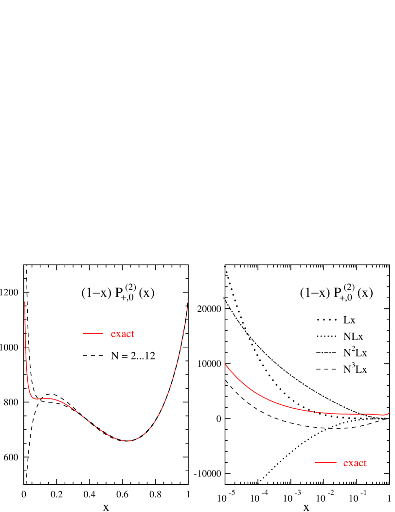
Figure 2: The $n_{\,\rm f\,}$-independent three-loop contribution $P_{+,0}^{\,(2)}(x)$ to the splitting function $P_{\rm ns}^{\,+}(x)$, multiplied by $(1-x)$ for display purposes. Also shown in the left part is the uncertainty band derived in Ref. [29] from the lowest six even-integer moments [24, 25, 26]. In the right part our exact result is compared to the small-$x$ approximations defined in Eq. (4.14) and the text below it.

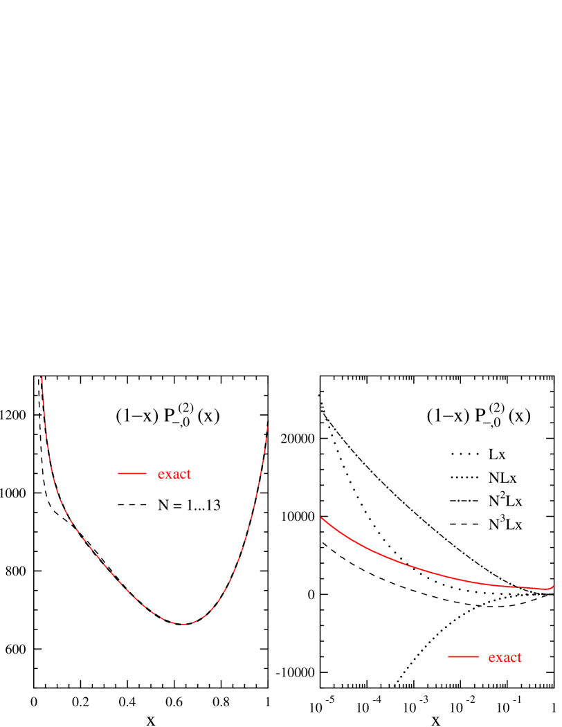
Figure 3: As Fig. 2, but for the splitting function $P_{\rm ns}^{\,-}(x)$. The first seven odd moments underlying the previous approximations [29] also shown in the left part have been computed in Ref. [26].

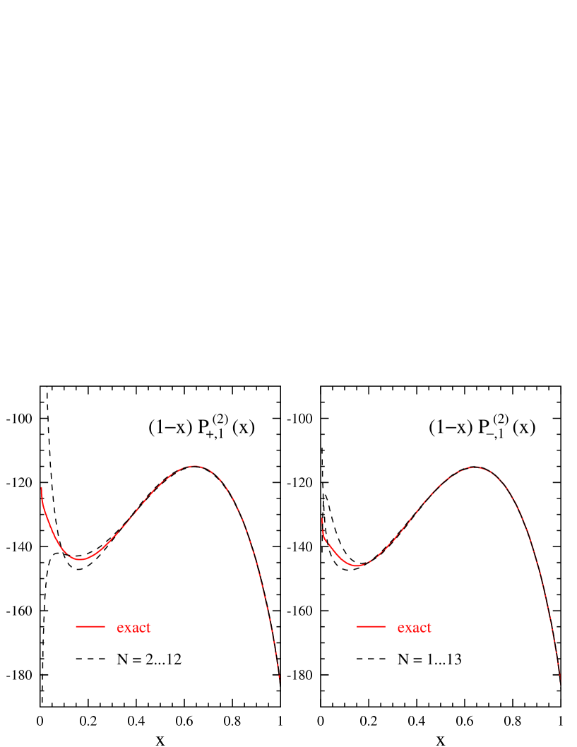
Figure 4: The $n_{\,\rm f\,}^{\,1}$ three-loop contributions $P_{\pm,1}^{\,(2)}(x)$ to the splitting functions $P_{\rm ns}^{\,\pm}(x)$, compared to the uncertainty bands of Ref. [29] based on the integer moments calculated in Refs. [24, 25, 26].

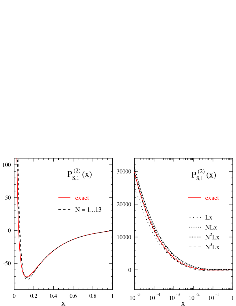
Figure 5: The first non-vanishing contribution $P_{{\rm s},1}^{\,(2)}(x)$ to the splitting functions $P_{\rm ns}^{\>s}(x)$, compared to the approximations of Ref. [29] (where, assuming the completeness of the resummation [30, 31], the possibility of a $\ln^{\,4}x$ term was disregarded) and to the small-$x$ expansion in powers of $\ln x$.

In view of the length and complexity of the exact expressions for the functions $P^{\,(2)i}_{\rm ns}(x)$, it is useful to have at ones disposal also compact approximate representations involving, besides powers of $x$, only simple functions like the $+$-distribution and the end-point logarithms

$${\cal D}_{\,0}\>=\>1/(1-x)_{+}\>,\quad L_{1}\>=\>\ln(1-x)\>,\quad L_{0}\>=\>\ln x\>\>.$$ (4.21)

Inserting the numerical values of the QCD colour factors, $P^{\,(2)+}_{\,\rm ns}$ in Eq. (4.9) can be represented by

$$P^{(2)+}_{\,\rm ns}(x)\!\!\! \cong \mbox{}\!\!+1174.898\>{\cal D}_{0}+1295.384\>\delta(1-x)+714.1\>L_{1}+1641.1-3135\>x+243.6\>x^{2}$$ (4.22)

$$\mbox{}\!\!-522.1\>x^{3}+L_{0}L_{1}[563.9+256.8\>L_{0}]+1258\>L_{0}+294.9\>L_{0}^{2}+800/27\>L_{0}^{3}+128/81\>L_{0}^{4}$$

$$+ \mbox{}{n_{\!f}}\>\Big{(}-183.187\>{\cal D}_{0}-173.927\>\delta(1-x)-5120/81\>L_{1}-197.0+381.1\>x+72.94\>x^{2}$$

$$\mbox{}\quad+44.79\>x^{3}-1.497\>xL_{0}^{3}-56.66\>L_{0}L_{1}-152.6\>L_{0}-2608/81\>L_{0}^{2}-64/27\>L_{0}^{3}\,\Big{)}$$

$$+ \mbox{}{n^{\,2}_{\!f}}\>\Big{(}-{\cal D}_{0}-(51/16+3\,{\zeta_{3}}-5\,{\zeta_{2}})\>\delta(1-x)+x\,(1-x)^{-1}L_{0}\,(3/2\>L_{0}+5)+1$$

$$\mbox{}\quad+(1-x)\,(6+11/2\>L_{0}+3/4\>L_{0}^{2})\,\Big{)}\>\,64/81\>\>.$$

A corresponding parametrization of $P^{\,(2)-}_{\,\rm ns}$ in Eq. (4.10) is given by

$$P^{(2)-}_{\,\rm ns}(x)\!\!\! \cong \mbox{}\!\!+1174.898\>{\cal D}_{0}+1295.470\>\delta(1-x)+714.1\>L_{1}+1860.2-3505\>x+297.0\>x^{2}$$ (4.23)

$$\mbox{}\!\!-433.2\>x^{3}+L_{0}L_{1}[684+251.2\>L_{0}]+1465.2\>L_{0}+399.2\>L_{0}^{2}+320/9\>L_{0}^{3}+116/81\>L_{0}^{4}$$

$$+ \mbox{}{n_{\!f}}\>\Big{(}-183.187\>{\cal D}_{0}-173.933\>\delta(1-x)-5120/81\>L_{1}-216.62+406.5\>x+77.89\>x^{2}$$

$$\mbox{}\quad+34.76\>x^{3}-1.136\>xL_{0}^{3}-65.43\>L_{0}L_{1}-172.69\>L_{0}-3216/81\>L_{0}^{2}-256/81\>L_{0}^{3}\,\Big{)}$$

$$+ \mbox{}{n^{\,2}_{\!f}}\>\Big{(}-{\cal D}_{0}-(51/16+3\,{\zeta_{3}}-5\,{\zeta_{2}})\>\delta(1-x)+x\,(1-x)^{-1}L_{0}\,(3/2\>L_{0}+5)+1$$

$$\mbox{}\quad+(1-x)\,(6+11/2\>L_{0}+3/4\>L_{0}^{2})\,\Big{)}\>\,64/81\>\>.$$

Finally the splitting function $P^{\,(2){\rm s}}_{\,\rm ns}$ in Eq. (4.11) can be approximated by

$$P^{(2)\rm s}_{\,\rm ns}(x)\!\! \cong {n_{\!f}}\>\Big{(}[\,L_{1}(-163.9\>x^{-1}-7.208\>x)+151.49+44.51\>x-43.12\>x^{2}+4.82\>x^{3}\,]\,[1-x\,]\quad$$ (4.24)

$$\mbox{}\!\!\!+L_{0}L_{1}[-173.1+46.18\>L_{0}]+178.04\>L_{0}+6.892\>L_{0}^{2}+40/27\>[L_{0}^{4}-2\>L_{0}^{3}\,]\,\Big{)}\>\ .\quad\quad$$

The identical ${n^{\,2}_{\!f}}$ parts of $P^{(2)\pm}_{\,\rm ns}$, the $+$-distribution contributions (up to a numerical truncation of the coefficients involving $\zeta_{i\,}$), and the rational coefficients of the (sub-)leading regular end-point terms are exact in Eqs. (4.22) – (4.24). The remaining coefficients have been determined by fits to the exact results, for which we have used the Fortran package of Ref. [75]. Except for $x$ values very close to zeros of $P^{(2)i}_{\rm ns}(x)$, the above parametrizations deviate from the exact expressions by less than one part in thousand, which should be sufficiently accurate for foreseeable numerical applications. For a maximal accuracy for the convolutions with the quark densities, also the coefficients of $\delta(1-x)$ have been slightly adjusted, by 0.02% or less, using low integer moments. Also the complex-$N$ moments of the splitting functions can be readily obtained to a perfectly sufficient accuracy using Eqs. (4.22) – (4.24). The Mellin transform of these parametrizations involve only simple harmonic sums $S_{m>0}(N)$ (see, e.g, the appendix of Ref. [60]) of which the analytic continuations in terms of logaritmic derivatives of Euler’s $\Gamma$-function are well known.

5 Numerical implications

In this section we illustrate the effect of our new three-loop splitting functions $P^{(2)\pm,\rm v}_{\,\rm ns}(x)$ on the evolution (2.6) of the non-singlet combinations $q_{\,\rm ns}^{\,\pm,\rm v}(x,\mu_{f}^{\,2})$ of the quark and antiquark distributions. For all figures we employ the same schematic, but characteristic model distribution,

$$xq_{\,\rm ns}^{\,\pm,\rm v}(x,\mu_{0}^{\,2})\>=\>x^{\,a}(1-x)^{b}\>\>$$ (5.1)

with

$$a\>=\>0.5\>\>,\quad b\>=\>3\>\>,$$ (5.2)

facilitating a direct comparison of the various splitting functions contributing to Eq. (2.6). For the same reason the reference scale is specified by an order-independent value for the strong coupling constant usually chosen as

$$\alpha_{\rm s}(\mu_{0}^{\,2})\>=\>0.2\>\>.$$ (5.3)

This value corresponds to $\mu_{0}^{\,2}\,\simeq\,25\ldots 50$ GeV² for $\alpha_{\rm s}(M_{Z}^{\,2})=0.114\ldots 0.120$ beyond the leading order, a scale region relevant for deep-inelastic scattering both at fixed-target experiments and, for much smaller $x$, at the ep collider HERA. Our default for the number of effectively massless flavours is ${n_{\!f}}=4$. The normalization of $q_{\,\rm ns}^{\>i}$ is irrelevant for our purposes, as we consider only the logaritmic derivatives $\dot{q}_{\rm ns}^{\>i}\equiv d\ln q_{\rm ns}^{\>i}/d\ln\mu_{f}^{\,2}$.

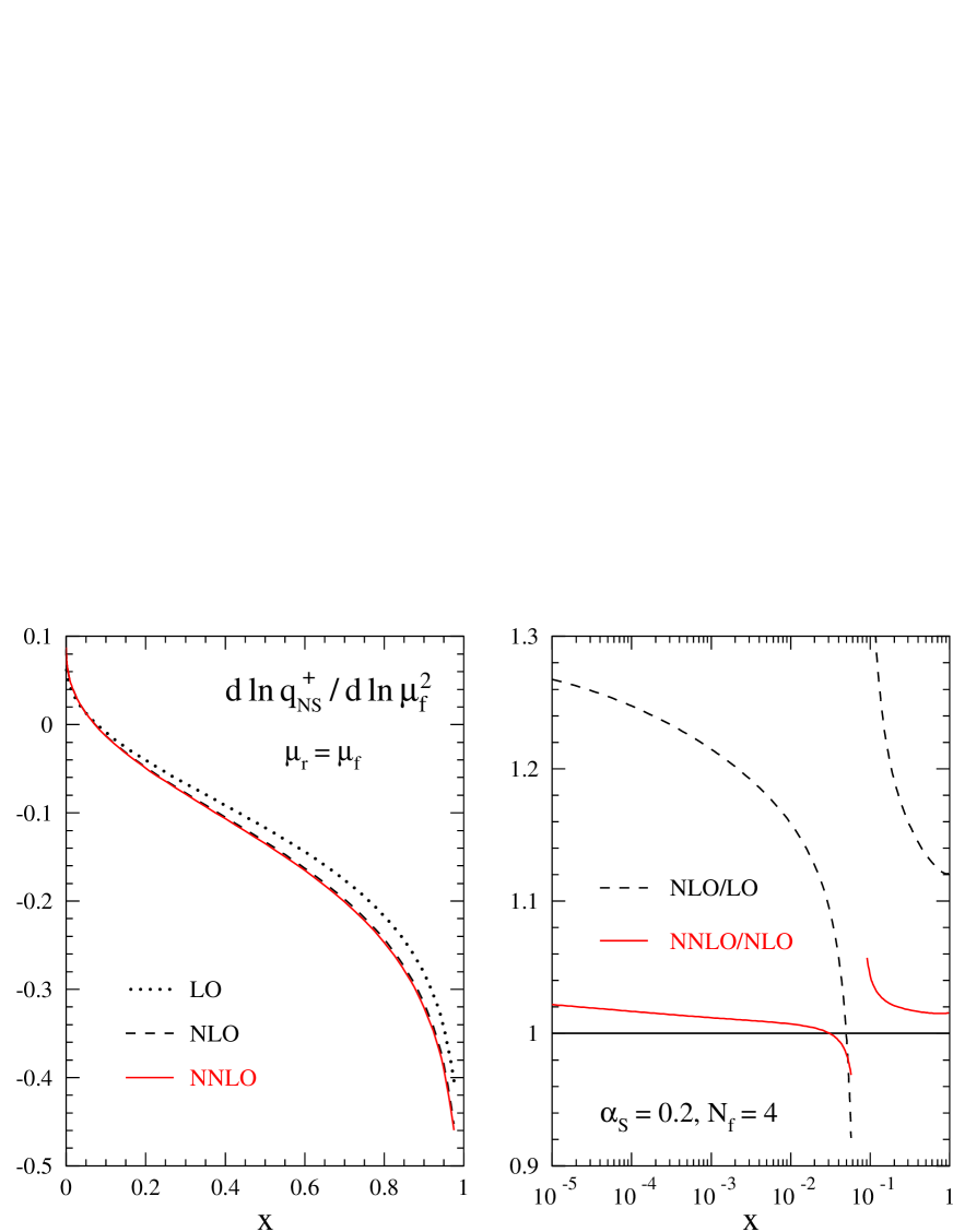
Figure 6: The perturbative expansion of the logarithmic scale derivative $\,d\ln q_{\,\rm ns}^{\,+}/d\ln\mu_{f}^{\,2}\,$ for a characteristic non-singlet quark distribution $xq_{\rm ns}^{\,+}\,=\,x^{\,0.5}(1-x)^{3}$ at the standard scale $\mu_{r}=\mu_{f}$.

Figure 7: As Fig. 6, but for the scale derivatives of the two other non-singlet combinations $q_{\,\rm ns}^{\,-,{\rm v}}$.

The scale derivatives of the three non-singlet distributions are graphically displayed in Figs. 6 and 7 over a wide region of $x$. At large $x$ the NNLO corrections are very similar in all cases, amounting to 2% or less for $x\geq 0.2$, thus being smaller than the NLO corrections by a factor of about eight. The same suppression factor is also found for $q_{\,\rm ns}^{\,-}(x)$ in the region $10^{-5}\raisebox{-1.9919pt}{$\>\>\stackrel{{\scriptstyle<}}{{{\scriptstyle\sim}}}\>\>$}x\raisebox{-1.9919pt}{$\>\>\stackrel{{\scriptstyle<}}{{{\scriptstyle\sim}}}\>\>$}10^{-2}$. The NNLO effects are even smaller for $q_{\,\rm ns}^{\,+}$ at small $x$, but considerably larger for $q_{\,\rm ns}^{\,\rm v}$ at $x<10^{-3}$. For example, at $x\simeq 10^{-4}$, where $P^{(2)\rm v}_{\rm ns}(x)$ exceeds $P^{(2)-}_{\rm ns}(x)$ by a factor of about 8 as discussed in the paragraph above Eq. (4.21), the ratio of the corresponding corrections in Fig. 7 amounts to 2.5. Recall that the scale derivatives (2.6) do not probe the splitting functions locally in $x$ due to the presence of the Mellin convolution.

The numerical values for $\dot{q}_{\rm ns}^{\>\rm v}(x,\mu_{0}^{\,2})$ are presented in Tab. 1 for four characteristic values of $x$. Also illustrated in this table is the dependence of the results on the shape of the initial distribution, the number of flavours and the value of the strong coupling constant. The relative corrections are rather weakly dependent of the large-$x$ power $b$ in Eq. (5.1). They increase at small $x$ with increasing small-$x$ power $a$, i.e., with decreasing size of $q_{\rm ns}^{\>\rm v}$. At large $x$, where the ${n_{\!f}}\,d^{abc\,}d_{abc}/n_{c}$ contribution $P^{\,\rm s}_{\,\rm ns}$ is negligible, the NNLO corrections decrease with increasing ${n_{\!f}}$. At small-$x$ this decrease is overcompensated in $\dot{q}_{\rm ns}^{\>\rm v}$ by the effect of $P^{\,\rm s}_{\rm ns}$. Except for very small momentum fractions $x\raisebox{-1.9919pt}{$\>\>\stackrel{{\scriptstyle<}}{{{\scriptstyle\sim}}}\>\>$}10^{-3}$ (where the non-singlet quark densities play a minor role for most important observables) the NNLO corrections amount to 15% or less even for a strong coupling constant as large as $\alpha_{\rm s}=0.5$. Hence the non-singlet evolution at intermediate and large $x$ appears to remain perturbative down to very low scales as used in the phenomenological analyses of Refs. [77, 78] and in non-perturbative studies of the initial distributions like those of Refs. [38, 39, 40, 41, 42, 43].

$x$	LO	NLO	NNLO	$r_{1}$	$r_{\,2}$	$r_{\,2}/r_{1}$
default (Fig. 7)
$10^{-4}$	$6.546\cdot 10^{-2}$	$8.424\cdot 10^{-2}$	$9.163\cdot 10^{-2}$	0.287	0.088	0.31
0.002	$5.632\cdot 10^{-2}$	$6.875\cdot 10^{-2}$	$7.041\cdot 10^{-2}$	0.221	0.024	0.11
0.25	$-5.402\cdot 10^{-2}$	$-6.331\cdot 10^{-2}$	$-6.457\cdot 10^{-2}$	0.172	0.020	0.12
0.75	$-1.949\cdot 10^{-1}$	$-2.189\cdot 10^{-1}$	$-2.222\cdot 10^{-1}$	0.123	0.015	0.12
$a=0.8$
$10^{-4}$	$1.660\cdot 10^{-1}$	$2.351\cdot 10^{-1}$	$2.818\cdot 10^{-1}$	0.417	0.198	0.48
0.002	$1.249\cdot 10^{-1}$	$1.583\cdot 10^{-1}$	$1.650\cdot 10^{-1}$	0.268	0.042	0.16
0.25	$-4.352\cdot 10^{-2}$	$-5.171\cdot 10^{-2}$	$-5.283\cdot 10^{-2}$	0.188	0.022	0.12
0.75	$-1.930\cdot 10^{-1}$	$-2.168\cdot 10^{-1}$	$-2.200\cdot 10^{-1}$	0.123	0.015	0.12
$b=5$
$10^{-4}$	$6.474\cdot 10^{-2}$	$8.278\cdot 10^{-2}$	$8.917\cdot 10^{-2}$	0.279	0.077	0.28
0.002	$5.324\cdot 10^{-2}$	$6.432\cdot 10^{-2}$	$6.546\cdot 10^{-2}$	0.208	0.018	0.09
0.25	$-7.835\cdot 10^{-2}$	$-9.022\cdot 10^{-2}$	$-9.180\cdot 10^{-2}$	0.151	0.018	0.12
0.75	$-2.300\cdot 10^{-1}$	$-2.580\cdot 10^{-1}$	$-2.619\cdot 10^{-1}$	0.122	0.015	0.12
${n_{\!f}}=3$
$10^{-4}$	$6.546\cdot 10^{-2}$	$8.480\cdot 10^{-2}$	$9.187\cdot 10^{-2}$	0.295	0.083	0.28
0.002	$5.632\cdot 10^{-2}$	$6.942\cdot 10^{-2}$	$7.174\cdot 10^{-2}$	0.233	0.033	0.14
0.25	$-5.402\cdot 10^{-2}$	$-6.406\cdot 10^{-2}$	$-6.588\cdot 10^{-2}$	0.186	0.028	0.15
0.75	$-1.949\cdot 10^{-1}$	$-2.219\cdot 10^{-1}$	$-2.269\cdot 10^{-1}$	0.139	0.023	0.16
${n_{\!f}}=3\>$ and $\>\alpha_{\rm s}=0.5$
$10^{-4}$	$1.636\cdot 10^{-1}$	$2.845\cdot 10^{-1}$	$3.949\cdot 10^{-1}$	0.739	0.388	0.53
0.002	$1.408\cdot 10^{-1}$	$2.227\cdot 10^{-1}$	$2.589\cdot 10^{-1}$	0.581	0.163	0.28
$0.25$	$-1.350\cdot 10^{-1}$	$-1.978\cdot 10^{-1}$	$-2.262\cdot 10^{-1}$	0.465	0.144	0.31
$0.75$	$-4.871\cdot 10^{-1}$	$-6.563\cdot 10^{-1}$	$-7.346\cdot 10^{-1}$	0.347	0.119	0.34

Table 1: The LO, NLO and NNLO logarithmic derivatives $\dot{q}_{\rm ns}^{\,\rm v}\equiv d\ln q_{\rm ns}^{\>v}/d\ln\mu_{f}^{\,2}$ at four representative values of $x$, together with the ratios $r_{n}={\rm N^{n}LO}/{\rm N^{n-1}LO}-1\,$ for the default input parameters specified in the first paragraph of this section and some variations thereof.

Another conventional way to assess the reliability of perturbative calculations is to investigate the stability of the results under variations of the renormalization scale $\mu_{r}$. For $\mu_{r}\neq\mu_{f}$ the expansion in Eq. (2.6) has to be replaced by

$$P_{\rm ns}^{\,i}(\mu_{f},\mu_{r}) \!=\! \quad a_{s}(\mu_{r}^{2})\,P_{\rm ns}^{(0)}\>\>+\>\>a_{s}^{2}(\mu_{r}^{2})\,\left(P_{\rm ns}^{(1),i}-\beta_{0}P_{\rm ns}^{(0)}\ln\frac{\mu_{f}^{2}}{\mu_{r}^{2}}\right)\>$$

$$\mbox{}\!\!\!+\>a_{s}^{3}(\mu_{r}^{2})\,\left(P_{\rm ns}^{(2),i}-\bigg{\{}\beta_{1}P_{\rm ns}^{(0)}+2\beta_{0}P_{\rm ns}^{(1),i}\bigg{\}}\ln\frac{\mu_{f}^{2}}{\mu_{r}^{2}}+\beta_{0}^{2}P_{\rm ns}^{(0)}\ln^{2}\frac{\mu_{f}^{2}}{\mu_{r}^{2}}\,\right)+\ldots\>\>,$$

where $\beta_{k}$ represent the $\overline{\mbox{MS}}$ expansion coefficients of the $\beta$-function of QCD  [79, 80, 81, 82].

In Fig. 8 the consequences of varying $\mu_{r}$ over the rather wide range $\frac{1}{8}\,\mu_{f}^{2}\,\leq\,\mu_{r}^{2}\,\leq\,8\mu_{f}^{2}$ are displayed for $\dot{q}_{\rm ns}^{\,+}$ at six representative values of $x$. The scale dependence is considerably reduced by including the third-order corrections over the full $x$-range. At NNLO both the points of fastest apparent convergence and the points of minimal $\mu_{r}$-sensitivity, $\partial\dot{q}_{\rm ns}^{\,+}/\partial\mu_{r}=0$, are rather close to the ‘natural’ choice $\mu_{r}=\mu_{f}$ for the renormalization scale.

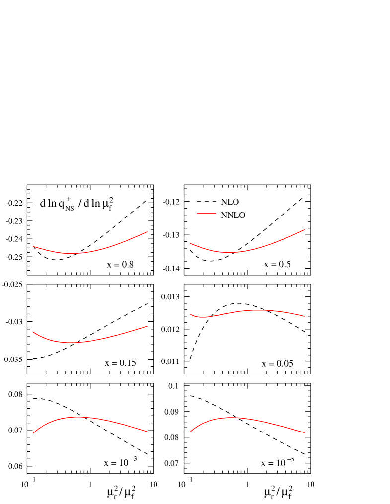
Figure 8: The dependence of the NLO and NNLO predictions for $\dot{q}_{\rm ns}^{\,+}\>\equiv\>d\ln q_{\rm ns}^{\,+}/d\ln\mu_{f}^{2}$ on the renormalization scale $\mu_{r}$ for six typical values of $x$. The initial conditions are as in Fig. 6.

The relative scale uncertainties of the average results, conventionally estimated by

$$\Delta\dot{q}_{\rm ns}^{\,i}\>\equiv\>\frac{\max\,[\dot{q}_{\rm ns}^{\,i}(x,\mu_{r}^{2}=\frac{1}{4}\mu_{f}^{2}\ldots 4\mu_{f}^{2})]-\min\,[\dot{q}_{\rm ns}^{\,i}(x,\mu_{r}^{2}=\frac{1}{4}\mu_{f}^{2}\ldots 4\mu_{f}^{2})]}{2\,|\,{\rm average}\,[\dot{q}_{\rm ns}^{\,i}(x,\mu_{r}^{2}=\frac{1}{4}\mu_{f}^{2}\ldots 4\mu_{f}^{2})]\,|}$$ (5.5)

is shown in Fig. 9 for all three cases $i=\pm,$v. These uncertainty estimates amount to 2% or less except for $x\raisebox{-1.9919pt}{$\>\>\stackrel{{\scriptstyle<}}{{{\scriptstyle\sim}}}\>\>$}10^{-3}$, an improvement by more than a factor of three with respect to the corresponding NLO results. Taking into account also the apparent convergence of the series in Figs. 6 and 7, it is not unreasonable to expect that the effect of the four-loop non-singlet splitting functions — which most likely will remain uncalculated for quite some time — will be less than 1% for $x>10^{-3}$. This expectation is consistent with the Padé estimates of $P_{\rm ns}^{\,(3)i}$ employed in Ref. [83] for the N³LO large-$x$ evolution of the deep-inelastic structure functions $F_{2}$ and $F_{3}$. At very small values of $x$ the higher-order corrections will presumably be considerably larger.

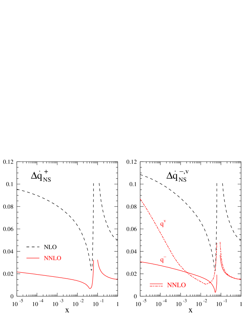
Figure 9: The renormalization scale uncertainty of the NLO and NNLO predictions for the scale derivative of $q_{\rm ns}^{\,i}$, $i=\pm,V$, as obtained from the quantity $\Delta\dot{q}_{\rm ns}^{\,i}$ defined in Eq. (5.5). Here and in Figs. 6 and 7 the spikes close to $x=0.1$ reflect the sign-change of $\dot{q}_{\rm ns}^{\,i}$ and do not constitute appreciable absolute corrections and uncertainties.

6 Summary

We have calculated the complete third-order contributions to the splitting functions governing the evolution of unpolarized non-singlet parton distribution in perturbative QCD. Our calculation is performed in Mellin-$N$ space and follows the previous fixed-$N$ computations [24, 25, 26] inasmuch as we compute the partonic structure functions in deep-inelastic scattering at even or odd $N$ using the optical theorem and a dispersion relation as discussed in [25]. Our calculation, however, is not restricted to low fixed values of $N$ but provides the complete $N$-dependence from which the $x$-space splitting functions can be obtained by a (by now) standard Mellin inversion. This progress has been made possible by an improved understanding of the mathematics of harmonic sums, difference equations and harmonic polylogarithms [59, 64, 45], and the implementation of corresponding tools, together with other new features [53], in the symbolic manipulation program Form [52] which we have employed to handle the almost prohibitively large intermediate expressions.

Our results have been presented in both Mellin-$N$ and Bjorken-$x$ space, in the latter case we have also provided easy-to-use accurate parametrizations. Our results agree with all partial results available in the literature, in particular we reproduce the lowest seven even- or odd-integer moments computed before [24, 25, 26]. We also agree with the resummation predictions [30, 31] for the leading small-$x$ logarithms $\ln^{\,4}x$ of the splitting functions $P_{\rm ns}^{\,+}(x)$ and $P_{\rm ns}^{\,-}(x)$ governing the evolution of flavour differences of quark-antiquark sums and differences. However, an unpredicted term of the same size is found also for the new $d^{abc\,}d_{abc}/n_{c}$ contributions $P_{\rm ns}^{\,\rm s}$ to the splitting function for the total valence distribution. At large $x$ we find that the coefficients of the leading integrable term $\ln(1-x)$ at order $n$ is proportional to the coefficient of the (only) $+$-distribution $1/(1-x)_{+}$ at order $n-1$, a result that seems to point to a yet unexplored structure.

We have investigated the numerical impact of the three-loop (NNLO) contributions on the evolution of the various non-singlet densities. The effect of the new contribution $P_{\rm ns}^{\,-}(x)$ is very small at large $x$ but rises sharply towards $x\rightarrow 0$, reaching 10% for a standard Regge-inspired $\sqrt{x}$ initial distributions at $x\simeq 10^{-5}$. At $x>10^{-3}$, on the other hand, the perturbative expansion for the scale dependences $d\ln q_{\rm ns}(x,\mu_{f}^{\,2})/d\ln\mu_{f}^{\,2}$ appear to be very well convergent. For $\alpha_{\rm s}=0.2$, for example, the NNLO corrections amount to 2% or less for four flavours, a factor of about 8 less than the NLO contributions. Also the variation of the renormalization scale leads to effects of about $\pm 2\%$ at NNLO in this region of $x$. Corrections of this size are comparable to the dependence of the predictions on the number of quark flavours, rendering a proper treatment of charm effects rather important even for large-$x$ non-singlet quantities, see Refs. [84, 85] and references therein.

Form files of our results, and Fortran subroutines of our exact and approximate $x$-space splitting functions can be obtained from the preprint server  http://arXiv.org by downloading the source. Furthermore they are available from the authors upon request.

Acknowledgments

The preparations for this calculation have been started by J.V. following a suggestion by S.A. Larin. For stimulating discussions during various stages of this project we would like to thank, in chronological order, S.A. Larin, F. J. Yndurain, E. Remiddi, E. Laenen, W. L. van Neerven, P. Uwer, S. Weinzierl and J. Blümlein. M. Zhou has contributed some Form routines during an early stage of the calculation. The work of S.M. has been supported in part by Deutsche Forschungsgemeinschaft in Sonderforschungsbereich/Transregio 9. The work of J.V. and A.V. has been part of the research program of the Dutch Foundation for Fundamental Research of Matter (FOM).

References

[1]
D.J. Gross and F. Wilczek,
Phys. Rev. D8 (1973) 3633
[2]
H. Georgi and H.D. Politzer,
Phys. Rev. D9 (1974) 416
[3]
G. Altarelli and G. Parisi,
Nucl. Phys. B126 (1977) 298
[4]
E.G. Floratos, D.A. Ross and C.T. Sachrajda,
Nucl. Phys. B129 (1977) 66
[5]
E.G. Floratos, D.A. Ross and C.T. Sachrajda,
Nucl. Phys. B152 (1979) 493
[6]
A. Gonzalez-Arroyo, C. Lopez and F.J. Yndurain,
Nucl. Phys. B153 (1979) 161
[7]
A. Gonzalez-Arroyo and C. Lopez,
Nucl. Phys. B166 (1980) 429
[8]
G. Curci, W. Furmanski and R. Petronzio,
Nucl. Phys. B175 (1980) 27
[9]
W. Furmanski and R. Petronzio,
Phys. Lett. 97B (1980) 437
[10]
E.G. Floratos, C. Kounnas and R. Lacaze,
Nucl. Phys. B192 (1981) 417
[11]
R. Hamberg and W.L. van Neerven,
Nucl. Phys. B379 (1992) 143
[12]
W.L. van Neerven and E.B. Zijlstra,
Phys. Lett. B272 (1991) 127
[13]
E.B. Zijlstra and W.L. van Neerven,
Phys. Lett. B273 (1991) 476
[14]
E.B. Zijlstra and W.L. van Neerven,
Phys. Lett. B297 (1992) 377
[15]
E.B. Zijlstra and W.L. van Neerven,
Nucl. Phys. B383 (1992) 525
[16]
R. Hamberg, W.L. van Neerven and T. Matsuura,
Nucl. Phys. B359 (1991) 343 [Erratum ibid. B 644 (2002) 403]
[17]
R.V. Harlander and W.B. Kilgore,
Phys. Rev. Lett. 88 (2002) 201801, hep-ph/0201206
[18]
C. Anastasiou, L. J. Dixon, K. Melnikov, and F. Petriello,
Phys. Rev. Lett. 91, 182002 (2003), hep-ph/0306192
[19]
C. Anastasiou, L. Dixon, K. Melnikov, and F. Petriello,
hep-ph/0312266.
[20]
C. Anastasiou and K. Melnikov,
Nucl. Phys. B646 (2002) 220, hep-ph/0207004
[21]
V. Ravindran, J. Smith and W.L. van Neerven,
Nucl. Phys. B665 (2003) 325, hep-ph/0302135