1 Introduction

LHC collaborations aimed at working in low and high $p_{T}$ regimes related to typical undulatory (diffractive) and corpuscular (point-like) behaviours of the corresponding cross-sections may offer a very exciting possibility to observe an interplay of both regimes [1]. In theory the ”hard part” can be (hopefully) treated with perturbative methods whilst the ”soft” one is definitely nonperturbative.

Below we give several examples of such an interplay: exclusive particle production by diffractively scattered protons, i.e. the processes $p+p\to p+X+p$, where $+$ means also a rapidity gap and X represents a particle or a system of particles consisting of or strongly coupled to the two-gluon state.

This process is related to the dominant amplitude of exclusive two-gluon production. Driving mechanism of the diffractive processes is the Pomeron. Data on the total cross-sections demands unambiguosly for the Pomeron with larger-than-one intercept, thereof the need in ”unitarisation”.

As will be seen below, EDDE gives us unique experimental possibilities for particle searches and investigations of diffraction itself. This is due to several advantages of the process: a) clear signature of the process; b) possibility to use ”missing mass method”, that improve the mass resolution; c) background is strongly suppressed; d) spin-parity analysis of the central system can be done; e) interesting measurements concerning the interplay between ”soft” and ”hard” scales are possible.

2 Calculations

In Figs. 1,2 we illustrate in detail the process $p+p\to p+X+p$. Off-shell proton-gluon amplitudes in Fig. 1 are treated by the method developed in Ref. [2], which is based on the extension of Regge-eikonal approach, and succesfully used for the description of the HERA data [3].

The amplitude of the process $p+p\to p+X+p$ can be obtained in the following way (see Figs. 1,2). The first step is to calculate the ”bare” amplitude $T_{X}$, which is depicted in Fig. 1. The ”hard” part is the usual gluon-gluon fusion process calculated by perturbative methods in the Standard Model or its extensions. ”Soft” amplitudes $T_{1,2}$ are obtained in the Regge-eikonal approach. The second step is the unitarization procedure, that takes into account initial and final state interactions (see Fig. 2).

We use the following kinematics, which corresponds to the double Regge limit. It is convenient to use light-cone components $(+,-;\bot)$. The components of momenta of the hadrons in Fig. 1 are

$$p_{1} = \left(\sqrt{\frac{s}{2}},\frac{m^{2}}{\sqrt{2s}},{\bf 0}\right)$$ (1)

$$p_{2} = \left(\frac{m^{2}}{\sqrt{2s}},\sqrt{\frac{s}{2}},{\bf 0}\right)$$

$$p_{1}^{\prime} = \left((1-\xi_{1})\sqrt{\frac{s}{2}},\frac{{\bf\Delta}_{1}^{2}+m^{2}}{(1-\xi_{1})\sqrt{2s}},-{\bf\Delta}_{1}\right)$$

$$p_{2}^{\prime} = \left(\frac{{\bf\Delta}_{2}^{2}+m^{2}}{(1-\xi_{2})\sqrt{2s}},(1-\xi_{2})\sqrt{\frac{s}{2}},-{\bf\Delta}_{2}\right)$$

$$q = \left(q_{+},q_{-},{\bf q}\right)\;{,}$$

$$q_{1} = q+p_{1}-p_{1}^{\prime}=q+\Delta_{1}\;{,}$$

$$q_{2} = -q+p_{2}-p_{2}^{\prime}=-q+\Delta_{2}\;{,}$$

$\xi_{1,2}$ are fractions of protons momenta carried by gluons. For two-dimensional transverse vectors we use boldface type. From the above notations we can obtain the relations:

$$t_{1,2}\;\;=\;\;\Delta_{1,2}^{2} \simeq -\frac{{\bf\Delta}_{1,2}^{2}(1+\xi_{1,2})+\xi_{1,2}^{2}m^{2}}{1-\xi_{1,2}}\;\;\simeq$$

$$\simeq -{\bf\Delta}_{1,2}^{2}\;{,}\;\;\xi_{1,2}\to 0$$

$$\cos\phi_{0} = \frac{{\bf\Delta}_{1}{\bf\Delta}_{2}}{|{\bf\Delta}_{1}||{\bf\Delta}_{2}|}$$

$$M_{X}^{2} \simeq \xi_{1}\xi_{2}s+t_{1}+t_{2}-2\sqrt{t_{1}t_{2}}\cos\phi_{0}$$

$$(p_{1}+q)^{2} \simeq m^{2}+q^{2}+\sqrt{2s}q_{-}=s_{1}$$

$$(p_{2}-q)^{2} \simeq m^{2}+q^{2}-\sqrt{2s}q_{+}=s_{2}\;.$$

Physical region of diffractive events with two rapidity gaps is defined by the following kinematical cuts:

$$0.01\;GeV^{2}\leq|t_{1,2}|\leq 1\;GeV^{2}\;{,}$$ (3)

$$\xi_{min}\simeq\frac{M_{X}^{2}}{s\xi_{max}}\leq\xi_{1,2}\leq\xi_{max}=0.1\;,$$ (4)

$$\left(\sqrt{-t_{1}}-\sqrt{-t_{2}}\right)^{2}\leq\! \kappa \!\leq\left(\sqrt{-t_{1}}+\sqrt{-t_{2}}\right)^{2}$$ (5)

$$\kappa=\xi_{1}\xi_{2}s\!\! - \!\!M_{X}^{2}\ll M_{X}^{2}$$

We can write the relations in terms of $y_{1,2}$ and $y_{X}$ (rapidities of hadrons and the system X correspondingly). For instance:

$$\xi_{1,2} \!\!\simeq\frac{M_{X}}{\sqrt{s}}e^{\pm y_{X}}\;,$$

$$|y_{X}| \!\!\leq y_{0}=\ln\left(\frac{\sqrt{s}\xi_{max}}{M_{X}}\right)\;,$$

$$y_{0}\simeq 2.5\! \!\sqrt{s}=14\;TeV\;{,}\;M_{X}=O(100\;GeV)\;,$$ for

$$|y_{1,2}| \!\!=\frac{1}{2}\ln\frac{(1-\xi_{1,2})^{2}s}{m^{2}-t_{1,2}}\geq 9$$

In standard terms the amplitude corresponds to the so-called nonfactorized scheme [4]. The contribution of the diagram depicted in Fig. 2 is obtained by integrating over all internal loop momenta. It was shown in [4], that the leading contribution arises from the region of the integration, where momentum $q$ is ”Glauber-like”, i.e. of the order $(\mbox{k}_{+}m^{2}/\sqrt{s},\mbox{k}_{-}m^{2}/\sqrt{s},\mbox{\bf k}m)$, where k’s are of the order $1$. The detailed consideration of the loop integral like

$$\int\frac{d^{4}q}{(2\pi)^{4}}\frac{f(q,p_{1},p_{2},\Delta_{1},\Delta_{2})}{(q^{2}+i0)(q_{1}^{2}+i0)(q_{2}^{2}+i0)}$$ (7)

shows that the main contribution comes from the poles at

$$q_{1}^{2} \!\!\!=\sqrt{2s}\xi_{1}q_{-}-{\mbox{\bf q}_{1}}^{2}=0\;,$$

$$q_{2}^{2} \!\!\!=-\sqrt{2s}\xi_{2}q_{+}-{\mbox{\bf q}_{2}}^{2}=0\;.$$

In this case

$$q=\left(-\frac{{\mbox{\bf q}_{2}}^{2}}{\xi_{2}\sqrt{2s}},\;\frac{{\mbox{\bf q}_{1}}^{2}}{\xi_{1}\sqrt{2s}},\mbox{\bf q}\right)\;{,}$$ (8)

where

$${\mbox{\bf q}_{1}}^{2} \!\!\!\!={\mbox{\bf q}}^{2}+{{\bf\Delta}_{1}}^{2}+2|\mbox{\bf q}||{\bf\Delta}_{1}|\cos(\phi+\frac{\phi_{0}}{2})\;{,}$$

$${\mbox{\bf q}_{2}}^{2} \!\!\!\!={\mbox{\bf q}}^{2}+{{\bf\Delta}_{2}}^{2}-2|\mbox{\bf q}||{\bf\Delta}_{2}|\cos(\phi-\frac{\phi_{0}}{2})$$

Taking the general form for $T$-amplitudes that satisfy identities

$$q^{\alpha}T^{D}_{\mu\alpha}=0,\;q_{i}^{\mu}T^{D}_{\mu\alpha}=0\;,$$ (9)

and neglecting terms of the order $o(\xi_{i})$, the following expression is found at $|t_{i}|\leq 1$ GeV²:

$$T^{D}_{\mu\alpha}(p,\;q,\;q_{i})=\left(G_{\mu\alpha}-\frac{P^{q_{i}}_{\mu}P^{q}_{\alpha}}{P^{q_{i}}P^{q}}\right)T^{D}_{gp\to gp}(s_{i},t_{i},qq_{i})$$ (10)

$$\noindent G_{\mu\alpha}=g_{\mu\nu}-\frac{q_{i,\mu}q_{\alpha}}{qq_{i}}\;,$$

$$\noindent P^{q_{i}}_{\mu}=p_{\mu}-\frac{pq_{i}}{qq_{i}}q_{\mu}\;,$$

$$\noindent P^{q}_{\alpha}=p_{\alpha}-\frac{pq}{qq_{i}}q_{i,\alpha}\;.$$

For $T^{D}_{gp\to gp}$ we use the Regge-eikonal approach [2, 5]. At small $t_{i}$ it takes the form of the Born approximation, i.e. Regge factor:

$$T^{D}_{gp\to gp}(s_{i},t_{i},qq_{i})=c_{gp}\left(e^{-i\frac{\pi}{2}}\frac{s_{i}-qq_{i}-m^{2}}{s_{0}-qq_{i}-m^{2}}\right)^{\alpha_{P}(t_{i})}e^{b_{0}t_{i}}\;,$$ (11)

$$b_{0}=\frac{1}{4}(\frac{r^{2}_{pp}}{2}+r^{2}_{gp})\;,$$

where $\alpha_{P}(0)=1.203$, $\alpha_{P}^{\prime}(0)=0.094$ GeV^-2, $r^{2}_{pp}=2.477$ GeV^-2 are fixed parameters for the ”hard” Pomeron [5], which have been obtained from the global fit to the data on diffractive $pp(p\bar{p})$ scattering. Parameters $c_{gp}\simeq 3.5$, $r^{2}_{gp}=2.54$ GeV^-2 are defined from fitting the HERA data on elastic $J/\Psi$ production [6], which will be published elsewhere. The upper bound for the constant $c^{up}_{gp}\simeq 2.3(3.3)$ can be also estimated from the exclusive double diffractive di-jet production at Tevatron (see (41)), if we take CDF cuts and the upper limit for the exclusive total di-jet cross-section [7]. The effective value $c_{gp}=2.3$ corresponds to the case, when the Sudakov suppression factor is absorbed into the constant, and $c_{gp}=3.3$ is obtained when taking into account this factor explicitely.

The full ”bare” amplitude looks as follows:

$$T_{pp\to pXp}\simeq\int\frac{d^{4}q}{(2\pi)^{4}}\frac{8F^{\mu\nu}(q_{1},q_{2})T^{D}_{\mu\alpha}(p_{1},\;q,\;q_{1})T^{D}_{\nu\alpha}(p_{2},\;-q,\;q_{2})}{(q^{2}+i0)(q_{1}^{2}+i0)(q_{2}^{2}+i0)}\;,$$ (12)

where

$$F^{\mu\nu}(q_{1},q_{2})=(g^{\mu\nu}-\frac{q_{2}^{\mu}q_{1}^{\nu}}{M_{X}^{2}})F_{gg\to X}\;.$$

Factor $8$ arises from the colour index contraction. Let $l^{2}=-q^{2}\simeq{\mbox{\bf q}}^{2}$, $y_{X}=<y_{X}>=0$ and contract all the tensor indices, then the integral (12) takes the form

$$T_{pp\to pXp}\simeq c_{gp}^{2}e^{b(t_{1}+t_{2})}\frac{\pi}{(2\pi)^{2}}\left(-\frac{s}{M_{X}^{2}}\right)^{\alpha_{P}(0)}\cdot 8F_{gg\to X}\cdot I\;,$$ (13)

$$b=\alpha^{\prime}_{P}(0)\ln\left(\frac{\sqrt{s}}{M_{X}}\right)+b_{0}\;,$$ (14)

$$I\simeq\int_{0}^{M_{X}^{2}}\frac{dl^{2}}{l^{4}}\left(\frac{l^{2}}{s_{0}-m^{2}+l^{2}/2}\right)^{2\alpha_{P}(0)}\;,$$ (15)

where $s_{0}-m^{2}\simeq 1$ GeV² is the scale parameter of the model that is used in the global fitting of the data on $pp(p\bar{p})$ scattering for on-shell amplitudes [5]. It remains fixed in the present calculations. It worth nothing that the ”rescattering corrections” for the off-shell gluon-proton amplitudes, $T^{D}$, are small (in accordance with a general analysis in Ref. [2]). Contrary to this, the ”outer” corrections (see Eq.(18)) are significant.

If we take into account the emission of virtual ”soft” gluons, while prohibiting the real ones, that could fill rapidity gaps, it results in the Sudakov-like suppression [8]:

$$F_{s}(l^{2})=exp\left[-\frac{3}{2\pi}\int\limits_{l^{2}}^{{M_{X}}^{2}/4}\frac{d{p_{T}}^{2}}{{p_{T}}^{2}}\alpha_{s}({p_{T}}^{2})\ln\left(\frac{{M_{X}}^{2}}{4{p_{T}}^{2}}\right)\right]\;,$$ (16)

and in the new value of the integral (15):

$$I_{s}\simeq\int_{0}^{M_{X}^{2}}\frac{dl^{2}}{l^{4}}F_{s}(l^{2})\left(\frac{l^{2}}{s_{0}-m^{2}+l^{2}/2}\right)^{2\alpha_{P}(0)}\;.$$ (17)

In this case the total cross-section becomes smaller, than without the factor $F_{s}$. It plays significant role for large $M_{X}$.

Unitarity corrections can be estimated from the elastic $pp$ scattering by the method depicted in Fig.2, where

$$T_{X} = T_{pp\to pXp}\;,$$ (18)

$$V(s\;,\;\mbox{\bf q}_{T}) = 4s(2\pi)^{2}\delta^{2}(\mbox{\bf q}_{T})+4s\int d^{2}\mbox{\bf b}e^{i\mbox{\bf q}_{T}\mbox{\bf b}}\left[e^{i\delta_{pp\to pp}}-1\right]\;,$$

$$T^{Unit.}_{X}(p_{1}\;,\;p_{2}\;,\;\Delta_{1}\;,\;\Delta_{2}) = \frac{1}{16ss^{\prime}}\int\frac{d^{2}\mbox{\bf q}_{T}}{(2\pi)^{2}}\frac{d^{2}\mbox{\bf q}^{\prime}_{T}}{(2\pi)^{2}}V(s\;,\;\mbox{\bf q}_{T})\;\cdot\;T_{X}(p_{1}-q_{T},p_{2}+q_{T},\Delta_{1T},\Delta_{2T})\;\cdot$$

$$\cdot \;V(s^{\prime}\;,\;\mbox{\bf q}^{\prime}_{T})\;,$$

$$\Delta_{1T} = \Delta_{1}-q_{T}-q^{\prime}_{T}\;,$$

$$\Delta_{2T} = \Delta_{2}+q_{T}+q^{\prime}_{T}\;,$$

and $\delta_{pp\to pp}$ can be found in Ref. [5]. These ”outer” unitarity corrections reduce the integrated cross-section by the factor about $14$ for the given kinematical cuts and lead to the changes in the $\phi_{0}$-dependence.

3 Results for resonance production

We have the following expression for the differential cross-section in case of one particle production:

$$\frac{d\sigma}{dt_{1}dt_{2}d\xi_{1}d\xi_{2}}\!\!\!\!\!\!\!\!\!\!\!\! =\frac{\pi|T^{Unit.}_{pp\to pXp}|^{2}}{8s(2\pi)^{5}\sqrt{-\lambda}}$$

$$\lambda =\kappa^{2}+2(t_{1}+t_{2})\kappa+(t_{1}-t_{2})^{2}\leq 0$$

By partial integrating (3) we obtain $t$ and $\xi$ distributions. The first result of our calculations is depicted in the Fig. 3. The antishrinkage of the diffraction peak with increasing mass $M_{X}$ is the direct consequence of the existence of the additional hard scale $M_{X}$, which makes the interaction radius smaller. The $\xi$ distribution is shown in Fig.4.

We can use the following replacement to obtain the cross-section for the EDD process $p+p\to p+X+p$:

$$|F_{gg\to X}|^{2}\to 4\pi M_{X}\Gamma(X\to gg)\;.$$ (20)

It is possible to simplify calculations after reduction of (3) to

$$\frac{d\sigma}{dt_{1}dt_{2}d\phi_{0}}\simeq\frac{\pi|T^{Unit.}_{pp\to pXp}|_{y_{X}=0}^{2}}{8s^{2}(2\pi)^{5}}\Delta y_{X}\;,$$ (21)

where $\Delta y_{X}=2y_{0}$, $\phi_{0}$ is the azimuthal angle between outgoing protons.

4 Standard model Higgs boson production

For the Standard Model Higgs boson [9]

$$\!\!F^{0}_{gg\to H} \!\!=\!\! M_{H}^{2}\frac{\alpha_{s}}{2\pi}\sqrt{\frac{G_{F}}{\sqrt{2}}}f(\eta)\;,$$ (22)

$$\!\!f(\eta) \!\!=\!\! \frac{1}{\eta}\left\{1+\frac{1}{2}\left(1-\frac{1}{\eta}\right)\left[Li_{2}\left(\frac{2}{1-\sqrt{1-\frac{1}{\eta}}-i0}\right)+Li_{2}\left(\frac{2}{1+\sqrt{1-\frac{1}{\eta}}+i0}\right)\right]\right\}\;,$$

$$|F_{gg\to H}|^{2} \to 1.5|F^{0}_{gg\to H}|^{2}\;,$$ (23)

where $\eta=M_{H}^{2}/4m_{t}^{2}$, $G_{F}$ is the Fermi constant, $m_{t}$ is the top quark mass. NLO K-factor 1.5 for the $gg\to H$ process is included to the final answer.

Numerical results are the following [10]

		$\sigma_{p+p\to p+H+p}$ (fb)
$c_{gp}$	$M_{H}$ (GeV)	LHC		TeVatron
		no Sud. suppr.	Sud. suppr.	no Sud. suppr.	Sud. suppr.
3.5	$100\to 500$	$110\to 57$	$4.6\to 0.14$	$12\to 0.4$	$0.5\to 0.001$
2.3(3.3)	$100\to 500$	$20\to 11$	$\mbox{\bf 3.6}\to\mbox{\bf 0.11}$	$2.2\to 0.08$	$0.4\to 0.0009$

We consider four different cases only for Higgs boson as illustration of the Sudakov suppressing action. In other examples we take $c_{gp}=3.3$ with Sudakov-like suppression according to the CDF data estimations to obtain the lower value of cross-sections at LHC and Tevatron. For this case our result is quite close to the one of [8], where the value of the total cross-section is about $3$ fb. In both cases the most important suppressing in the mass region $M_{H}>100$ GeV is due to (perturbative) Sudakov factors, while the nonperturbative (absorbtive) factors play relatively minor role.

Results of other authors were considered in details in [11]. Here we refer to the highest cross-section $2$ pb for $M_{H}=400$ GeV at LHC energies that was obtained in Ref. [12]. A nonfactorized form of the amplitude and a ”QCD inspired” model for $gp\to gp$ amplitudes were used, taking into account the nonperturbative proton wave functions. Even if we multiply the result of Ref. [12] by the suppressing factor, it will be larger than ours. This could serve as the indication of the role of nonperturbative effects. Our model is based on the Regge-eikonal approach for the amplitudes, which is primordially nonperturbative, normalized to the data from HERA on $\gamma p\to J/\Psi p$ [6] and improved by the CDF data on the exclusive di-jet production [7].

To estimate the signal to QCD background ratio for $b\bar{b}$ signal we use the standard expression for $gg\to b\bar{b}$ amplitude and assumptions [13]-[16]:

• possibility to separate final $b\bar{b}$ quark jets from gluon jets. If we cannot do it, it will increase the background by two orders of magnitude under the $50\%$ efficiency.

• suppression due to the absence of colour-octet $b\bar{b}$ final states

• suppression of light fermion pair production, when $J_{z,tot}=0$ (see also [17],[18])

• cut $E_{T}>50$ GeV ($\theta\geq 60^{\mbox{\small o}}$), since the cross-section of EDD $b\bar{b}$ jet production strongly decreases with $E_{T}$ (see formulae (39)).

The theoretical result of our numerical estimations is

$$\frac{Signal(pp\to pHp\to pb\bar{b}p)}{QCD\;\;background}\geq 3.8\frac{GeV}{\Delta M}\;{,}$$ (24)

where $\Delta M$ is the mass resolution of the detector and $M_{H}\simeq 115$ GeV, which can reach $0.01M_{H}$ due to application of the ”missing mass method”. Similar result was strictly obtained in [13],[14]. Under the above circumstances the total efficiency at the integrated luminocity $30$ fb^-1 is $\sim 10\%$ and numerically estimated significance of the event is about $3\sigma$, which is close to the one in $\gamma\gamma$ decay mode.

5 Heavy quarkonium production

Results for $\chi_{c0,b0}$ EDD production were obtained recently by some authors [13],[15],[19] in different approaches. To obtain the total cross-sections in the model considered in the present paper let us substitute widths of these states into (20).

$$\Gamma(\chi_{b0}\to gg)\simeq\Gamma_{0}(\chi_{b0}\to gg)\left(1+9.8\frac{\alpha_{S}}{\pi}\right)=550\;keV\;\mbox{(see \cite[cite]{[\@@bibref{}{Khozebg1chi}{}{}]},\cite[cite]{[\@@bibref{}{KhozeJz0chi}{}{}]} for details)},$$ (25)

where the width is set to the lattice result $\Gamma_{0}(\chi_{b0}\to gg)=354\;keV$ [20]. After replacement we obtain for LHC and TeVatron:

$$\sigma_{pp\to p+\chi_{b0}+p}\simeq 1.3\;nb\;,\sqrt{s}=14\;TeV\;,\;\mbox{((\ref{tlimits}),(\ref{xlimits}) cuts),}$$ (26)

$$\sigma_{pp\to p+\chi_{b0}+p}\simeq 160\;pb\;,\sqrt{s}=1.8\;TeV\;,\;\mbox{(CDF cuts),}$$ (27)

The same procedure can be done for $\chi_{c0}$. Taking the total width $\Gamma(\chi_{c0}\to gg)\simeq 14.9\;MeV$ [21] we obtain

$$\sigma_{pp\to p+\chi_{c0}+p}\simeq 4\;\mu b\;,\sqrt{s}=14\;TeV\;,\;\mbox{((\ref{tlimits}),(\ref{xlimits}) cuts),}$$ (28)

$$\sigma_{pp\to p+\chi_{c0}+p}\simeq 600\;nb\;,\sqrt{s}=1.8\;TeV\;,\;\mbox{(CDF cuts).}$$ (29)

6 Radion production.

Now there is a great interest to the multidimensional properties of the space-time. One of the models was proposed by Randall and Sundrum [22]. We have considered the case of one compact extra-dimension. In this case we have additional scalar particle Radion, that reflects the existence of an extra dimension and represents the field of the ”distance” oscillations between the branes along the extra dimension. Since Radion has the same quantum numbers as the Higgs boson, they can mix [23]. After mixing we have two mass eigenstates, which could be observed experimentally. For the EDDE the following replacements in (22) should be done:

$$f(\eta) \to a_{34}f(\eta_{h^{*}})+7\gamma\;b\;\;\mbox{for}\;h^{*}\;,$$ (30)

$$f(\eta) \to \gamma\left(a_{12}f(\eta_{r^{*}})+7a\right)\;\;\mbox{for}\;r^{*}\;,$$ (31)

where $\eta_{h^{*},r^{*}}=m_{h^{*},r^{*}}^{2}/4m_{t}^{2}$ and other parameters are obtained from formulae in the Appendix A of [23]:

$$\gamma=v/\Lambda_{\phi}\;,v=246\;GeV\;\mbox{is the Higgs VEV}\;,\;\Lambda_{\phi}\;\mbox{is the radion VEV}\;,$$ (32)

$$Z^{2}=1-6\xi\gamma^{2}(1+6\xi)\;,\;\tan 2\theta=12\xi\gamma Z\frac{1}{Z^{2}-36\xi^{2}\gamma^{2}-m^{2}_{r}/m^{2}_{h}}\;,$$ (33)

$$a=\cos\theta/Z\;;\;b=-\sin\theta/Z\;;\;c=\sin\theta-6\xi\gamma/Z\;;\;d=\cos\theta+6\xi\gamma/Z\;\sin\theta\;,$$ (34)

$$a_{12}=a+c/\gamma\;;\;a_{34}=d+b\gamma\;,$$ (35)

$$m^{2}_{r^{*}}=c^{2}m^{2}_{h}+a^{2}m^{2}_{r}\;;\;m^{2}_{h^{*}}=d^{2}m^{2}_{h}+b^{2}m^{2}_{r}\;,$$ (36)

$$r=ar^{*}+bh^{*}\;;\;h=cr^{*}+dh^{*}\;.$$ (37)

Results for the total cross-sections in the case of $c_{gp}=3.3$ with Sudakov-like suppression are depicted in Figs.5,6 for several values of mixing parameter $\xi$ and for the vacuum expectation value of the radion field $\Lambda_{\phi}=1$ TeV.

7 EDD dijet production

For the EDD production of a dijet system of mass $M_{X}$ in the leading order (see, for example [4]) we have:

$$|F_{gg\to X}|^{2}\to\frac{144\pi^{2}\alpha_{S}^{2}M_{X}^{4}}{E_{T}^{4}}\;,X=gg\;,$$ (38)

$$|F_{gg\to X}|^{2}\to\frac{32\pi^{2}\alpha_{S}^{2}M_{X}^{2}m_{Q}^{2}}{3E_{T}^{4}}\beta^{2}\;,X=Q\bar{Q}\;,\beta=\sqrt{1-4m_{Q}^{2}/M_{X}^{2}}\;,$$ (39)

and the cross-section becomes

$$\frac{d\sigma}{dt_{1}dt_{2}dy_{X}d\kappa^{\prime}dE_{T}^{2}}\simeq\frac{|T^{Unit.}_{pp\to pjjp}|^{2}}{2^{13}\pi^{5}s^{2}\kappa^{\prime}\sqrt{1-\kappa^{\prime}}}\;,$$ (40)

where $\kappa^{\prime}=4E_{T}^{2}/M_{X}^{2}$, and $T^{Unit.}_{pp\to pjjp}$ is calculated as in the section 2 with substitutions (38),(39).

Note that all the results of this article are given for the value of the constant $c_{gp}=3.3$, which is obtained from the upper bounds for the exclusive di-jet production at TeVatron energies [7]. Cross-sections and numerical estimations for $c_{gp}$ at different transverse energy cuts are the following:

$$E_{T}> \!\!7\;GeV\;, \sigma<3.7\;nb\;,\;c_{gp}<3.3$$ (41)

$$E_{T}> \!\!10\;GeV\;, \sigma<0.97\pm 0.065\;(stat.)\pm 0.272(sys.)\;nb\;,\;c_{gp}<3.4$$

$$E_{T}> \!\!25\;GeV\;, \sigma<34\pm 5\;(stat.)\pm 10(sys.)\;pb\;,\;c_{gp}<4.2\;.$$

The lowest value is close to the result, obtained by fitting the HERA data on elastic $J/\Psi$ production. It can serve as the indication of model applicability.

From the analogous calculations for LHC with cuts (3),(4) we have:

$$E_{T}>10\;GeV, \sigma(pp\to p+jet+jet+p)\simeq 7\;nb$$ (42)

$$E_{T}>25\;GeV, \sigma(pp\to p+jet+jet+p)\simeq 150\;pb$$

$$E_{T}>50\;GeV, \sigma(pp\to p+jet+jet+p)\simeq 8\;pb.$$

8 Conclusions

We see from the results that there is a real possibility to use advantages of the the EDDE for investigations at LHC. Accuracy of the mass measurements could be improved by applying the missing mass method [24].

The low value of the exclusive Higgs boson production cross-section obtained in this paper is mainly due to the Sudakov suppression factor (16), the full validity of which is not obvious, because the confinement effects can strongly modify the ”real gluon emission”. It is interesting that in spite of different models and quite different ways of account of absorbtive effects in our paper and in Ref. [8], the final results appeared to be quite close.

Certainly, the cross-sections may be several times larger due to still not very well known non-perturbative factors.

In the case of heavy quarkonium and dijet EDD production cross-sections are much larger than for Higgs boson production, and some other important investigations like measurements of the azimuthal angle dependence and the diffractive pattern of the interaction could be done.

Aknowledgements

We are grateful to A. De Roeck, A. Prokudin, A. Rostovtsev, N.E. Tyurin, A. Sobol, S. Slabospitsky and participants of BLOIS2003 workshop and several CMS meetings for helpful discussions. We are also indebted to N.V. Krasnikov and V.A. Matveev, who draw our attention to the radion phenomenology. This work is supported by the Russian Foundation for Basic Research, grant no. 02-02-16355

Figure captions

• 1: The process $p+p\to p+X+p$. Absorbtion in the initial and final pp-channels is not shown.

• 2: The full unitarization of the process $p+p\to p+X+p$.

• 3: t-distribution $d\sigma/dt/\sigma_{tot}$ of the process $p+p\to p+X+p$ for masses of the system X equal to 100 and 500 GeV.

• 4: $\xi$-distribution $d\sigma/d\xi/\sigma_{tot}$ of the process $p+p\to p+X+p$ for $M_{X}=100$ GeV.

• 5: The total cross-section (in fb) of the process $p+p\to p+h*+p$ versus Higgs boson($h^{*}$) mass for $c_{gp}=3.3$ with Sudakov-like suppression at LHC. Parameters of RS1 model are shown.

• 6: The total cross-section (in fb) of the process $p+p\to p+r*+p$ versus Radion($r^{*}$) mass for $c_{gp}=3.3$ with Sudakov-like suppression at LHC. Parameters of RS1 model are shown.

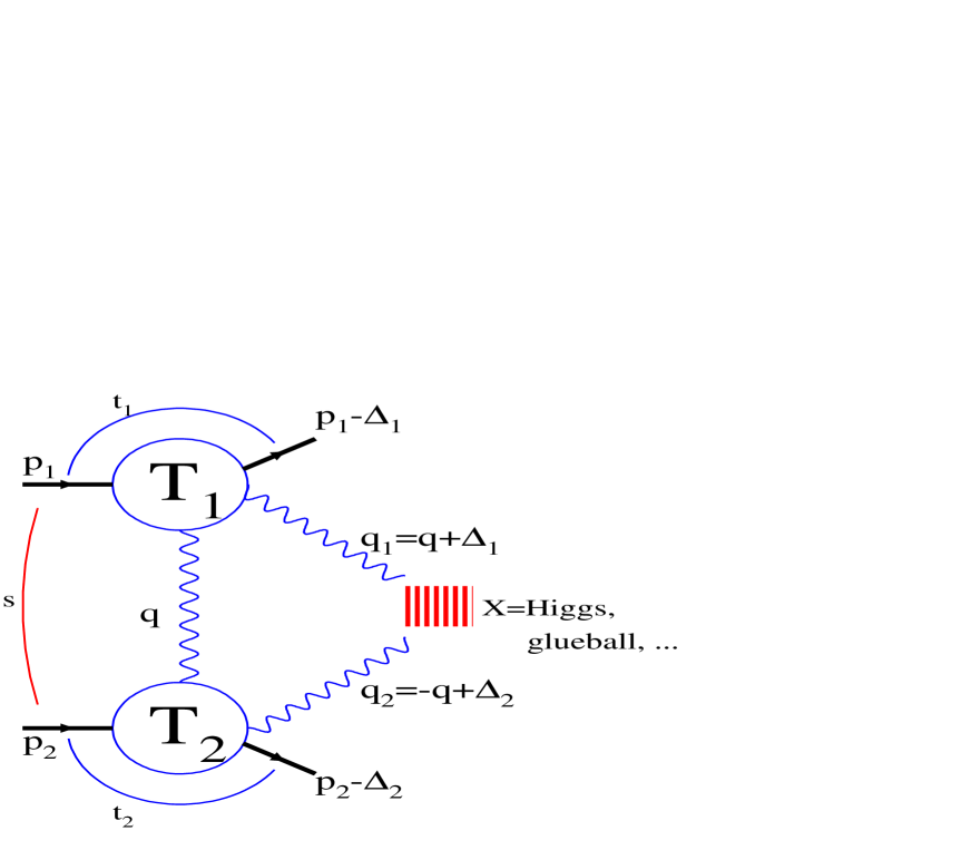
Figure 1:

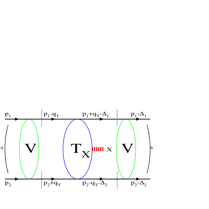
Figure 2:

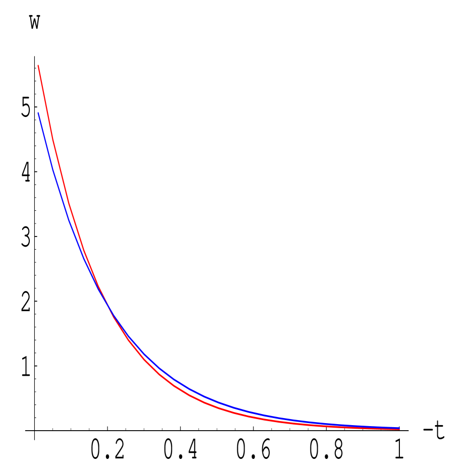
Figure 3:

Figure 4:

Figure 5:

Figure 6:

References

• [1] V.A. Petrov, Proc. of the 2nd Int. Symp. ”LHC: Physics and Detectors”. (Eds. A.N. Sissakian and Y.A. Kultchitsky), June 2000, Dubna. P.223;
V.A. Petrov, A.V. Prokudin, S.M. Troshin, N.E. Tyurin, J. Phys. G: Nucl. Part. Phys. 27 (2001) 2225.
• [2] V.A. Petrov, Proceedings of the VIIth Blois Wokshop (Ed. M. Haguenauer et al., Editions Fronti$\grave{e}$res; Paris 1995).
• [3] V.A. Petrov and A.V. Prokudin, Phys. Atom. Nucl. 62 (1999) 1562.
• [4] A. Berera and J. C. Collins, Nucl. Phys. B 474 (1996) 183.
• [5] V.A. Petrov and A. V. Prokudin, Eur. Phys. J. C 23 (2002)135.
• [6] S. Aid et al. H1 Collab. Nucl. Phys. B 472 (1996) 3, hep-ex/9603005;
C.Adloff et al. H1 Collab. Phys. Lett. B 483 (2000) 23, hep-ex/0003020;
ZEUS Collab. Z. Phys. C 75 (1997) 215, hep-ex/9704013;
ZEUS Collab. Phys. Lett. B 437 (1998) 432, hep-ex/9807020.
• [7] CDF Collaboration (K. Borras for the collaboration). FERMILAB-CONF-00-141-E, Jun 2000; K. Goulianos, talk given in the Xth Blois workshop, 2003, Helsinki, Finland.
M. Gallinaro, hep-ph/0311192.
• [8] V. A. Khoze, A. D. Martin and M. G. Ryskin, Eur. Phys. J. C 14 (2000) 525;
Eur. Phys. J. C 21 (2001) 99; V. A. Khoze, hep-ph/0105224;
• [9] A. Kniehl, Phys. Rept. 240 (1994) 211.
• [10] V.A. Petrov and R.A. Ryutin, hep-ph/0311024, submitted to Eur.Phys.J.C.
• [11] V. A. Khoze, A. D. Martin, M. G. Ryskin, Eur. Phys. J. C 26 (2002) 229.
• [12] J.-R. Cudell and O. F. Hernandez, Nucl. Phys. B 471 (1996) 471.
• [13] V. A. Khoze, A. D. Martin, M. G. Ryskin, Eur. Phys. J. C 19 (2001) 477.
• [14] A. De Roeck,V. A. Khoze, A. D. Martin, R. Orava, M. G. Ryskin, Eur. Phys. J. C 25 (2002) 391.
• [15] V. A. Khoze, A. D. Martin, M. G. Ryskin, Eur. Phys. J. C 23 (2002) 311.
• [16] A. D. Martin, M. G. Ryskin and V. A. Khoze, Phys. Rev. D 56 (1997) 5867.
• [17] A. Bialas and V. Szeremeta, Phys. Lett. B 296 (1992) 191;
A. Bialas and R. Janik, Z. Phys. C 62 (1994) 487.
• [18] J. Pumplin, Phys. Rev. D 52 (1995) 1477.
• [19] Feng Yuan, Phys. Lett. B 510 (2001) 155.
• [20] S. Kim, Nucl. Phys. B (Proc. Suppl.) 471 (1996) 437.
• [21] Review of Particle Properties, Eur. Phys. J. C 15 (2000) 1.
• [22] L. Randall and R. Sundrum, Phys. Rev. Lett. 83 (1999) 3370.
• [23] M. Chaichian, A. Datta, K. Huitu and Zenghui Yu, Phys.Lett. B524 (2002) 161
• [24] M.G. Albrow and A. Rostovtsev, FERMILAB-PUB-00-173. Aug. 2000.