GLUEBALL-GLUEBALL INTERACTION IN THE CONTEXT
OF AN EFFECTIVE THEORY

Abstract

In this work we use a mapping technique to derive in the context of a constituent gluon model an effective Hamiltonian that involves explicit gluon degrees of freedom. We study glueballs with two gluons using the Fock-Tani formalism.

Received (received date)Revised (revised date)

1 Introduction

The gluon self-coupling in QCD implies the existence of bound states of pure gauge fields known as glueballs. Numerous technical difficulties have so far been present in our understanding of their properties in experiments, largely because glueball states can mix strongly with nearby $q\bar{q}$ resonances. However recent experimental and lattice studies of $0^{++}$, $2^{++}$ and $0^{-+}$ glueballs seem to be convergent. In the present we follow a different approach by applying the Fock-Tani formalism in order to obtain an effective interaction between glueballs [1]. A glueball-glueball cross-section can be obtained and compared with usual meson-meson cross-sections.

2 Fock-Tani Formalism for Glueballs

The starting point is the creation operator of a glueball formed by two constituent gluons

$$G_{\alpha}^{\dagger}=\frac{1}{\sqrt{2}}\Phi_{\alpha}^{\mu\nu}a_{\mu}^{\dagger}a_{\nu}^{\dagger}$$

where gluons obey the following commutation relations

$$[a_{\mu},a_{\nu}]=0\,\,\,\,;\,\,\,\,[a_{\mu},a_{\nu}^{\dagger}]=\delta_{\mu\nu}$$

The composite glueball operator satisfy non-canonical commutation relations

$$[G_{\alpha},G_{\beta}]=0\,\,\,\,\,;\,\,\,\,[G_{\alpha},G_{\beta}^{\dagger}]=\delta_{\alpha\beta}+\Delta_{\alpha\beta}$$

where

$$\delta_{\alpha\beta}=\Phi_{\alpha}^{\star\rho\gamma}\Phi_{\beta}^{\gamma\rho}\,\,\,\,\,\,;\,\,\,\,\,\,\Delta_{\alpha\beta}=2\Phi_{\alpha}^{\star\mu\gamma}\Phi_{\beta}^{\gamma\rho}a_{\rho}^{\dagger}a_{\mu}$$

The Fock-Tani formalism introduces “ideal particles” which obey canonical relations, in our case they are ideal glueballs

$$[g_{\alpha},g_{\beta}]=0\,\,\,\,\,;\,\,\,\,[g_{\alpha},g_{\beta}^{\dagger}]=\delta_{\alpha\beta}$$

This way one can transform the composite glueball state $|\alpha\rangle$ into an ideal state $|\alpha\,)$ by

$$|\alpha\,)=U^{-1}(-\frac{\pi}{2})\,G_{\alpha}^{\dagger}\,|0\rangle=g_{\alpha}^{\dagger}\,|0\rangle$$

where $U=\exp({tF})$ and $F$ is the generator of the glueball transformation given by

$$F=g_{\alpha}^{\dagger}\tilde{G}_{\alpha}-\tilde{G}_{\alpha}^{\dagger}g_{\alpha}$$ (1)

with

$$\tilde{G}_{\alpha}=G_{\alpha}-\frac{1}{2}\Delta_{\alpha\beta}G_{\beta}-\frac{1}{2}G_{\beta}^{\dagger}[\Delta_{\beta\gamma},G_{\alpha}]G_{\gamma}$$

In order to obtain the effective glueball-glueball potential one has to use (1) in a set of Heisenberg-like equations for the basic operators $g,\tilde{G},a$

$$\frac{dg_{\alpha}(t)}{dt}=[g_{\alpha},F]=\tilde{G}_{\alpha}\,\,\,\,\,;\,\,\,\,\,\frac{d\tilde{G}_{\alpha}(t)}{dt}=[\tilde{G}_{\alpha}(t),F]=-g_{\alpha}\,.$$

The simplicity of these equations are not present in the equations for $a$

$$\frac{da_{\mu}(t)}{dt}=[a_{\mu},F]= - \sqrt{2}\Phi_{\beta}^{\mu\nu}a_{\nu}^{\dagger}g_{\beta}+\frac{\sqrt{2}}{2}\Phi_{\beta}^{\mu\nu}a_{\nu}^{\dagger}\Delta_{\beta\alpha}g_{\beta}$$

$$+ \Phi_{\alpha}^{\star\mu\gamma}\Phi_{\beta}^{\gamma\mu^{{}^{\prime}}}(G_{\beta}^{\dagger}a_{\mu^{{}^{\prime}}}g_{\beta}-g_{\beta}^{\dagger}a_{\mu^{{}^{\prime}}}G_{\beta})$$

$$- \sqrt{2}(\Phi_{\alpha}^{\mu\rho^{{}^{\prime}}}\Phi_{\rho}^{\mu^{{}^{\prime}}\gamma^{{}^{\prime}}}\Phi_{\gamma}^{\star\gamma^{{}^{\prime}}\rho^{{}^{\prime}}}+\Phi_{\alpha}^{\mu^{{}^{\prime}}\rho^{{}^{\prime}}}\Phi_{\rho}^{\mu\gamma^{{}^{\prime}}}\Phi_{\gamma}^{\star\gamma^{{}^{\prime}}\rho^{{}^{\prime}}})G_{\gamma}^{\dagger}a_{\mu^{{}^{\prime}}}^{\dagger}G_{\beta}g_{\beta}$$

The solution for these equation can be found order by order in the wavefunctions. So, for zero order one has $a_{\mu}^{(0)}=a_{\mu}$

$$g_{\alpha}^{(0)}(t)=G_{\alpha}\sin{t}+g_{\alpha}\cos{t}\,\,\,\,;\,\,\,\,G_{\beta}^{(0)}(t)=G_{\beta}\cos{t}-g_{\beta}\sin{t}$$

In the first order $g_{\alpha}^{(1)}=0,\,\,\,G_{\beta}^{(1)}=0$ and

$$a_{\mu}^{(1)}(t)=\sqrt{2}\Phi_{\beta}^{\mu\nu}a_{\nu}^{\dagger}[G_{\beta}^{(0)}-G_{\beta}]$$

In the second order we found

$$a_{\mu}^{(2)}(t)=-2\Phi_{\alpha}^{\star\mu\gamma}\Phi_{\beta}^{\gamma\mu^{{}^{\prime}}}G_{\beta}^{\dagger}a_{\mu^{{}^{\prime}}}G_{\alpha}^{(0)}+\Phi_{\alpha}^{\star\mu\gamma}\Phi_{\beta}^{\gamma\mu^{{}^{\prime}}}G_{\beta}^{\dagger}a_{\mu^{{}^{\prime}}}G_{\alpha}+\Phi_{\alpha}^{\star\mu\gamma}\Phi_{\beta}^{\gamma\mu^{{}^{\prime}}}G_{\beta}^{\dagger(0)}a_{\mu^{{}^{\prime}}}G_{\alpha}^{(0)}$$

To obtain the third order $a_{\mu}^{(3)}(t)$ is straightforward and shall be presented elsewhere. The glueball-glueball potential can be obtained applying in a standard way the Fock-Tani transformed operators to the microscopic Hamiltonian

$${\cal{H}}(\mu\nu;\sigma\rho)=T_{\rm aa}(\mu)a_{\mu}^{\dagger}a_{\mu}+\frac{1}{2}V_{\rm aa}(\mu\nu;\sigma\rho)a_{\mu}^{\dagger}a_{\nu}^{\dagger}a_{\rho}a_{\sigma}$$

where one obtains for the glueball-gluball potential $V_{gg}$

$$V_{gg}=\sum_{i=1}^{4}V_{i}(\alpha\gamma;\delta\beta)g_{\alpha}^{\dagger}g_{\gamma}^{\dagger}g_{\delta}g_{\beta}$$ (2)

and

$$V_{1}(\alpha\gamma;\delta\beta)=2V_{aa}(\mu\nu;\sigma\rho)\Phi_{\alpha}^{\star\mu\tau}\Phi_{\gamma}^{\star\nu\xi}\Phi_{\delta}^{\rho\xi}\Phi_{\beta}^{\sigma\tau}$$

$$V_{2}(\alpha\gamma;\delta\beta)=2V_{aa}(\mu\nu;\sigma\rho)\Phi_{\alpha}^{\star\mu\tau}\Phi_{\gamma}^{\star\nu\xi}\Phi_{\delta}^{\rho\tau}\Phi_{\beta}^{\sigma\xi}$$

$$V_{3}(\alpha\gamma;\delta\beta)=V_{aa}(\mu\nu;\sigma\rho)\Phi_{\alpha}^{\star\mu\nu}\Phi_{\gamma}^{\star\lambda\xi}\Phi_{\delta}^{\sigma\lambda}\Phi_{\beta}^{\rho\xi}$$

$$V_{4}(\alpha\gamma;\delta\beta)=V_{aa}(\mu\nu;\sigma\rho)\Phi_{\alpha}^{\star\mu\xi}\Phi_{\gamma}^{\star\nu\lambda}\Phi_{\delta}^{\lambda\xi}\Phi_{\beta}^{\rho\sigma}\,.$$

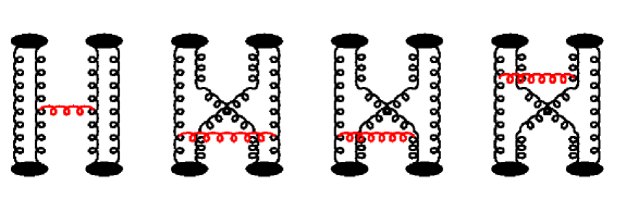
Figure 1: Diagrams representing the scattering amplitude $h_{fi}$ for glueball-glueball interaction with constituent gluon interchange.

The next step is to obtain the scattering $T$-matrix from Eq. (2)

$$T(\alpha\beta;\gamma\delta)=(\alpha\beta|V_{gg}|\gamma\delta)\,.$$

Due to translational invariance, the $T$-matrix element is written as a momentum conservation delta-function, times a Born-order matrix element, $h_{fi}$: $T(\alpha\beta;\gamma\delta)=\delta^{(3)}(\vec{P}_{f}-\vec{P}_{i})\,h_{fi}$, where $\vec{P}_{f}$ and $\vec{P}_{i}$ are the final and initial momenta of the two-glueball system. This result can be used in order to evaluate the glueball-glueball scattering cross-section

$$\sigma_{gg}=\frac{4\pi^{5}\,s}{s-4M_{G}^{2}}\int_{-(s-4M_{G}^{2})}^{0}\,dt\,|h_{fi}|^{2}$$ (3)

where $M_{G}$ is the glueball mass, $s$ and $t$ are the Mandelstam variables.

3 The Constituent Gluon Model

On theoretical grounds, a simple potential model with massive constituent gluons, namely the model of Cornwall and Soni [2],[3] has been studied [4],[5] and the results are consistent with lattice and experiment. In the conventional quark model a $0^{++}$ state is considered as $q\bar{q}$ bound state. The $0^{++}$ resonance is a isospin zero state so, in principal, it can be either represented as a $q\bar{q}$ bound state, a glueball, or a mixture. In particular there is growing evidence in the direction of large $s\bar{s}$ content with some mixture with the glue sector. It turns out that this resonance is an interesting system, in the theoretical point of view, where one can compare models. In the present work we consider two possibilities for $0^{++}$: (i) a as pure $s\bar{s}$ and calculate, in the context of a quark interchange picture, the cross-section; (ii ) as a glueball where a new calculation for this cross-section is made, in the context of the constituent gluon model, with gluon interchange. The potential $V_{\rm aa}$ is determined in the Cornwall and Soni constituent gluon model [2]

$$V_{\rm aa}(r)=\frac{1}{3}\,f^{ace}f^{bde}\left[\,V_{2g}^{OGEP}(r)+V_{S}(r)\right]$$ (4)

where

$$V_{2g}^{OGEP}(r)=-\lambda\,\left[\,\omega_{1}\frac{e^{-mr}}{r}+\omega_{2}\frac{\pi}{m^{2}}\,D(r)\,\right]\,\,\,\,\,\,,\,\,\,\,\,\,V_{S}(r)=2m\,(1-e^{-\beta\,m\,r})$$ (5)

and

$$D(r)=\frac{k^{3}m^{3}}{\pi^{3/2}}\,e^{-k^{2}m^{2}r^{2}}\,\,\,\,\,\,,\,\,\,\,\,\,\lambda=\frac{3\,g^{2}}{4\pi}\,\,\,\,\,\,,\,\,\,\,\,\,\omega_{1}=\frac{1}{4}+\frac{1}{3}\vec{S}^{2}\,\,\,\,\,\,,\,\,\,\,\,\,\omega_{2}=1-\frac{5}{6}\vec{S}^{2}.$$ (6)

The parameters $\lambda$, $m$, $k$ and $\beta$ assume known values[3, 4, 5] while the wave function $\Phi^{\mu\nu}_{\alpha}$ is given in [6]. The glueball-glueball scattering amplitude $h_{fi}$ is given by

$$h_{fi}(s,t) = \frac{3}{8}\,R_{0}(s)\sum_{i=1}^{6}\,R_{i}(s,t)$$ (7)

where

$$R_{0} = \frac{4}{(2\pi)^{3/2}b^{3}}\exp\left[-\frac{1}{2b^{2}}\left(\frac{s}{4}-M_{G}^{2}\right)\right]$$

$$R_{1} = \frac{\lambda\omega_{1}^{(2)}\,4\,\sqrt{2\pi}}{3}\,\int_{0}^{\infty}dq\,\frac{q^{2}}{q^{2}+m^{2}}\exp\left(-\frac{q^{2}}{2b^{2}}\right)\left[{\mathcal{J}}_{0}\left(\frac{q\sqrt{t}}{2b^{2}}\right)+{\mathcal{J}}_{0}\left(\frac{q\sqrt{u}}{2b^{2}}\right)\right]$$

$$R_{2} = \frac{\lambda\omega_{2}^{(2)}2\sqrt{2}\pi b^{3}k^{3}m}{3(b^{2}+2k^{2}m^{2})^{3/2}}\left[\exp\left(-\frac{tk^{2}m^{2}}{4(b^{4}+2b^{2}k^{2}m^{2})}\right)+\exp\left(-\frac{uk^{2}m^{2}}{4(b^{4}+2b^{2}k^{2}m^{2})}\right)\right]$$

$$R_{3} = \frac{32\sqrt{2\pi}}{3}\int_{0}^{\infty}dq\,\frac{q^{2}\beta m^{2}}{(q^{2}+\beta^{2}m^{2})^{2}}\exp\left(-\frac{q^{2}}{2b^{2}}\right)\left[{\mathcal{J}}_{0}\left(\frac{q\sqrt{t}}{2b^{2}}\right)+{\mathcal{J}}_{0}\left(\frac{q\sqrt{u}}{2b^{2}}\right)\right]$$

$$R_{4} = -\frac{\lambda\omega_{1}^{(3)}}{3}\,\,\frac{16\,\sqrt{2\pi}\,b^{2}}{\sqrt{\frac{s}{4}-M_{G}^{2}}}\int_{0}^{\infty}dq\,\frac{q}{q^{2}+m^{2}}\exp\left(-\frac{3q^{2}}{8b^{2}}\right)\sinh\left(\frac{q}{2b^{2}}\sqrt{\frac{s}{4}-M_{G}^{2}}\,\right)$$

$$R_{5} = -\frac{\lambda\omega_{2}^{(3)}\,}{3}\,\frac{16\pi b^{3}k^{3}m}{(2b^{2}+3k^{2}m^{2})^{3/2}}\exp\left[-\frac{k^{2}m^{2}\left(\frac{s}{4}-M_{G}^{2}\right)}{2(2b^{4}+3b^{2}k^{2}m^{2})}\right]$$

$$R_{6} = -\frac{128\sqrt{2\pi}b^{2}}{3\sqrt{\frac{s}{4}-M_{G}^{2}}}\int_{0}^{\infty}dq\,\frac{q\beta m^{2}}{(q^{2}+\beta^{2}m^{2})^{2}}\exp\left(\frac{3q^{2}}{8b^{2}}\right)\sinh\left(\frac{q}{2b^{2}}\sqrt{\frac{s}{4}-M_{G}^{2}}\,\right)$$ (8)

here $b=\frac{\sqrt{3}}{\sqrt{2}\,r_{0}}$ where $r_{0}$ is the glueball’s rms radius and ${\cal J}_{0}(x)=\sin x/x$. In (8) one finds the following notation $\omega^{(i)}_{1}$ and $\omega^{(i)}_{2}$, where the index $i$ correponds to the number of the evaluated diagram in figure (1) The cross-section is obtained inserting (7) in (3). From reference [6] one obtains the corresponding cross-section for a $0^{++}$ meson with a $s\bar{s}$ content

$$\sigma_{fi}^{s\bar{s}}=\frac{4\pi\alpha_{s}^{2}s}{81m_{q}^{4}}\left[\frac{4b^{2}\left(1-e^{-\frac{\xi}{4b^{2}}}\right)}{\xi}+\frac{128}{27}e^{-\frac{\xi}{6b^{2}}}+e^{-\frac{\xi}{8b^{2}}}+\frac{64}{3\sqrt{3}}\frac{4b^{2}}{\xi}\left(e^{-\frac{\xi}{12b^{2}}}-e^{-\frac{5\xi}{24b^{2}}}\right)\right]\;$$

with $\xi=s-4M_{G}^{2}$. The comparison between the cross-sections in the glueball picture and the quark picture for the $0^{++}$ meson is given in figure (2).

file=cross0pp.eps, height=300.00pt, width=200.00pt,angle=-90

Figure 2: Cross-section comparison for $0^{++}$ with the following parameters $\beta=0.1$, $\lambda=1.8$, $k=0.21$, gluon mass $m=0.6$GeV. The $s\bar{s}$ quark model parameters: $m_{q}=0.55$ GeV, $\alpha_{s}=0.6$.

4 Conclusions

In this work we have extended the Fock-Tani Formalism to a hadronic model in which the bound state is composed by bosons. The Cornwall-Soni constituent gluon model has been successful in describing low mass glueballs, in particular the $0^{++}$ resonance, which is a isospin zero state. This state can be either represented as a $q\bar{q}$ bound state, a glueball, or a mixture. In the present work we have considered two possibilities for $0^{++}$: a as pure $s\bar{s}$ and as a glueball. A comparison of the cross-sections reveals that a quark composition for the $0^{++}$ implies in a larger rms radius than in the constituent gluon picture. This could represent a criterion for distinguishing between pictures.

References

- [1] Hadjimichef D, Krein G, Szpigel S and Veiga J S da Ann. of Phys. 268 105 (1998).
- [2] Cornwall J M and Soni A Phys. Lett. 120B, 431 (1983).
- [3] Hou W S and Soni A Phys. Rev. D29, 101 (1984).
- [4] Hou W S, Luo C S and Wong G G Phys. Rev. D64, 014028 (2001).
- [5] Hou W S and Wong G G Phys. Rev. D67, 034003 (2003).
- [6] Szpigel S Interação Méson-Méson no Formalismo Fock-Tani. PhD thesis (Doutorado em Ciências) - Instituto de Física, Universidade de São Paulo, São Paulo, 1995.