Radiative B decays in Supersymmetry without R𝑅R-parity

Otto C. W. Kong and Rishikesh D. Vaidya
Department of Physics, National Central University,
Chung-Li 32054 Taiwan.
Abstract

We present a systematic analysis of all the contributions at the leading log order to the branching ratio of the inclusive radiative decay Bβ†’Xs+γ→𝐡subscript𝑋𝑠𝛾B\rightarrow X_{s}+\gammaΒ in the framework of supersymmetry without R𝑅R-parity. The relevant set of four-quark operators involved in QCD running are extended from 6 (within SM and MSSM) to 24, with also many new contributions to the Wilson coefficients of (chromo)magnetic penguins for either chiral structure. We present complete analytical results here without any a priori assumptions on the form of R𝑅R-parity violation. Mass eigenstate expressions are given, hence the results are free from the commonly adopted mass-insertion approximation. In the numerical analysis, we focus here only on the influence of the trilinear Ξ»i​j​kβ€²subscriptsuperscriptπœ†β€²π‘–π‘—π‘˜\lambda^{\prime}_{ijk} couplings and report on the possibility of a few orders of magnitude improvement for the bounds on a few combinations of the Ξ»β€²superscriptπœ†β€²\lambda^{\prime} couplings. Our study shows that the Wilson coefficients of the current-current operators due to R𝑅R-parity violation dominate over the direct contributions to the penguins. However, the inter-play of various contributions is complicated due to the QCD corrections which we elaborate here.

††preprint: NCU-HEP-k014 Feb 2004 rev. Aug 2004

I Introduction

With the successful testing of the gauge sector during the LEP era, the standard model (SM) of particle physics has certainly established itself as an essentially correct theory at and below the GeV scale. However, it still leaves many basic issues to be investigated. Even if one forgets about the hierarchy problem, and the need for neutrino masses, a cursory look at the error bars of about 20 % on the various flavor parameters pdg2 , and their wide range of apparently arbitrary numerical values suggests that the flavor sector is still much of a misery. Within flavor physics, it is the phenomena of the flavor changing neutral currents (FCNCs) that could be the window of the physics beyond SM. Forbidden at the tree level due to the unitarity of VCKMsubscript𝑉CKMV_{\mbox{\tiny CKM}}, FCNCs are loop induced where exotic virtualities (from supersymmetry or otherwise) could pop up and hence completely change the predictions for the decay rate. This could prove to be complementary to the direct search of the exotic particles by hinting toward a particular class of models or by ruling out large regions in the parameter space of beyond SM models, and thus, guiding the accelerator searches.

Among the FCNCs, the process Bβ†’Xs+γ→𝐡subscript𝑋𝑠𝛾B\rightarrow X_{s}+\gammaΒ is particularly attractive, both theoretically as well as experimentally. From the point of view of theory, though the calculation is very complicated and was a major challenge due to the ambiguities following β€˜scheme dependence’ of the decay rate right at the leading log (LL) bsg_classics ; cella , it was worth an effort. Unlike many hadronic processes, it can largely be freed from the scale and scheme dependence within the framework of renormalization group improved perturbation theory and heavy mass expansion together with the assumption of quark-hadron duality. All this is possible because mb>>Ξ›Q​C​Dmuch-greater-thansubscriptπ‘šπ‘subscriptΛ𝑄𝐢𝐷m_{b}>>\Lambda_{\scriptscriptstyle QCD} and hence, the inclusive decay Bβ†’Xs+γ→𝐡subscript𝑋𝑠𝛾B\rightarrow X_{s}+\gammaΒ  is very well approximated by the corresponding partonic level transition bβ†’s+γ→𝑏𝑠𝛾b\rightarrow s+\gammaΒ where the non-perturbative pathogens play only sub-leading role being suppressed by at least two powers of mbsubscriptπ‘šπ‘m_{b} (the corrections are less than 10%). The next to leading log (NLL) result for the branching fraction in the case of SM is given as gam-mis-01 ; bur-mis-02 :

B​r​[Bβ†’Xs+γ​(EΞ³>1.6​G​e​V)]SM=(3.57Β±0.30)Γ—10βˆ’4.π΅π‘Ÿsubscriptdelimited-[]→𝐡subscript𝑋𝑠𝛾subscript𝐸𝛾1.6𝐺𝑒𝑉SMplus-or-minus3.570.30superscript104Br\left[B\rightarrow X_{s}+\gamma\;(E_{\gamma}>1.6GeV)\right]_{\scriptscriptstyle\mathrm{SM}}=(3.57\pm 0.30)\times 10^{-4}\;. (1)

Here, EΞ³subscript𝐸𝛾E_{\gamma} is the energy cut on the photon spectrum to get rid of the background photons. The above result implies that this particular β€˜rare’ decay is actually not so rare. This is because, unlike other rare decays, where the rate is ∝GF2​αQ​E​D2proportional-toabsentsubscriptsuperscript𝐺2𝐹subscriptsuperscript𝛼2𝑄𝐸𝐷\propto G^{2}_{\scriptscriptstyle F}\alpha^{2}_{\scriptscriptstyle QED}, here it is ∝GF2​αQ​E​Dproportional-toabsentsubscriptsuperscript𝐺2𝐹subscript𝛼𝑄𝐸𝐷\propto G^{2}_{\scriptscriptstyle F}\alpha_{\scriptscriptstyle QED}. Also due to the heavy top in the loop, GIM suppression is not much effective. The high rate has already been quite well measured by CLEO cleo_bsg , BELLE belle_bsg and ALEPH aleph_bsg . The results of different experiments are consistent with each other. A weighted average of the available experimental measurement is problematic, because the model dependence errors (and also the systematic errors) are correlated and differ within the various measurements. An analysis taking into account the correlations, leads to the following world average world_average

B​r​[Bβ†’Xs+γ​(EΞ³>1.6​G​e​V)]EXP=(3.34Β±0.38)Γ—10βˆ’4.π΅π‘Ÿsubscriptdelimited-[]→𝐡subscript𝑋𝑠𝛾subscript𝐸𝛾1.6𝐺𝑒𝑉EXPplus-or-minus3.340.38superscript104Br\left[B\rightarrow X_{s}+\gamma\;(E_{\gamma}>1.6GeV)\right]_{\scriptscriptstyle\mathrm{EXP}}=(3.34\pm 0.38)\times 10^{-4}\;. (2)

Within 1ΟƒπœŽ\sigma it matches the SM predictions gam-mis-01 ; bur-mis-02 . So it is clear that there is not much room for new physics contributions111See the note added in proof at the end.. Either the new physics contributions are negligible, or there are large cancellations among various contributions. Thus, a study of new physics contributions can help to reduce the viable regions in parameter space of the relevant model. This channel is indeed very well studied in the most popular theory of beyond SM physics, namely the minimal supersymmetric standard model (MSSM) mssm ; baer ; carena . There is already a vast literature on the topic and we are not adding to that here. The imposed baryon number (B) and lepton number (L) conservation (in the form of R𝑅R-parity) within MSSM, is totally ad hoc. It is an overkill of a problem of proton decay which can be easily rescued by alternatives like baryon parity. It also forbids the neutrino masses that would otherwise arise naturally. In fact, super-symmetrizing the SM with its sacred gauge symmetries and renormalizability, one naturally lands into the generic supersymmetric standard model or the supersymmetry (SUSY) without R𝑅R-parity otto-gssm . However, due to the presence of a large number of free parameters, any phenomenological study of R𝑅R-parity violation (RPV) models is a daunting task. On the other hand, one may consider the origin and suppression of these parameters as due to a spontaneously broken anomalous Abelian family symmetry which is invoked to understand the fermion mass hierarchies fn . In ref.u1 such an attempt is made to understand the pattern of R𝑅R-parity violation consistent with phenomenology at the electroweak scale. However, in the absence of a compelling model of the kind, it is imperative that all possible phenomenological constraints on these,a priori, free parameters be studied. Such complexity necessitates a careful examination of the exact definition of the RPV couplings, and the choice of an optimal parametrization of the latter, or rather the full model Lagrangian, that can simplify the structure of mass matrices to enable an analytical diagonalization in a suitable approximation. The single vev parametrization (SVP), first explicitly advocated in otto-svp is such a parametrization. In this paper, we investigate the RPV contributions from the generic model to the process bβ†’s+γ→𝑏𝑠𝛾b\rightarrow s+\gammaΒ within the framework of SVP bsg-icfp . We give analytical formulae that include all possible contributions without a priori assumption on the form of R-parity violation. In the same spirit as an earlier study on ΞΌβ†’e+Ξ³β†’πœ‡π‘’π›Ύ\mu\rightarrow e+\gamma otto-mueg , we give mass eigenstate expressions, hence free from the commonly adopted mass-insertion approximation. In the numerical analysis, we focus in this paper only on the influence of the trilinear Ξ»i​j​kβ€²subscriptsuperscriptπœ†β€²π‘–π‘—π‘˜\lambda^{\prime}_{ijk} couplings and report on the possibility of a few orders of magnitude improvement for the bounds on a few combination of Ξ»i​j​kβ€²subscriptsuperscriptπœ†β€²π‘–π‘—π‘˜\lambda^{\prime}_{ijk} parameters. Our formulation also has the advantage that the physical meaning of the Ξ»β€²superscriptπœ†β€²\lambda^{\prime}-couplings would not change at all, whether the numerical values of any of the other RPV parameters are vanishingly small or otherwise.

There have been some studies on the process within the general framework of R𝑅R-parity violation. More systematic analysis are exemplified by refs.carlos ; besmer . Ref.carlos , fails to consider the additional 18 four-quark operators which, in fact, give the dominant contribution in most of the cases. As we shall demonstrate, the interplay of various contributions along with the QCD corrections, is very complicated and hence various contributions could add up or cancel depending on a particular case. The more recent work of ref.besmer has considered a complete operator basis. However, we find their formula for Wilson coefficient incomplete, and they do not report on the possibility of a few orders of magnitude improvement on the bounds for certain combinations of RPV couplings, as we present here. We must mention here that around the same time as ref.besmer authors of ref.chun-bsg published an analysis of the CP-asymmetries in the radiative B-decays, which involved a similar calculation machinery with the extended operator basis. To the best of our knowledge all the available studies on the topic in the literature, in fact are incomplete or incorrect to some extent. This is mostly a problem of incomplete consideration for the RPV couplings of the bilinear type and the mass mixings the latter produce in the sectors of fermions and scalars. We present here a complete treatment of the full operator basis together with the corresponding Wilson coefficients under the truly generic and consistent formulation of SUSY without R𝑅R-parity. In fact, the existence of interesting contributions from combinations of bilinear and trilinear RPV couplings in the process has been noted in the earlier studies of the model under the SVP formulation otto-jhep ; kong-keum . We present the full analytical result here. However, due to other complications involved, we will postpone any numerical study on the aspect to a later publication. Focusing our attention here on the trilinear RPV parameters, we perform our analysis at the leading log order. Such an approximation entails uncertainties of about 25 %. However, owing to sensitive dependence of the result on the large number of input parameters, we consider it worth-while to examine the relevant parameter space and obtain order of magnitude bounds before performing any precision analysis.

The paper is organized as follows: In section II we briefly summarize the main features of SVP parametrization and also set our notation. Section III deals with the effective Hamiltonian formulation, the extended operator basis and the Wilson coefficients. Section IV discusses the decay rate calculation in relation to the anomalous dimension matrix and the renormalization group running of the full set of 28 operators. We discuss our major numerical results in section V, and conclude the paper after. Some details involving the full set of 28 operators and the 28Γ—28282828\times 28 anomalous dimension matrix is left to an appendix. The numerical results discussed here are restricted to those obtained from combinations trilinear couplings along. Contributions from combinations of a trilinear and a bilinear parameter, the latter going into the loop diagrams through RPV mass mixings, form another class of novel results essentially not studied before. We present that latter part, from our parallel study, in an independent publication017 .

II The Single VEV Parametrization

The most general renormalizable superpotential for the generic supersymmetric SM (without R𝑅R-parity) can be written as

Wπ‘Š\displaystyle W\!\!\!\! =\displaystyle= Ξ΅a​b​[μα​H^ua​L^Ξ±b+hi​ku​Q^ia​H^ub​U^kC+λα​j​k′​L^Ξ±a​Q^jb​D^kC+12​λα​β​k​L^Ξ±a​L^Ξ²b​E^kC]+12​λi​j​k′′​U^iC​D^jC​D^kC,subscriptπœ€π‘Žπ‘delimited-[]subscriptπœ‡π›Όsuperscriptsubscript^π»π‘’π‘Žsuperscriptsubscript^𝐿𝛼𝑏superscriptsubscriptβ„Žπ‘–π‘˜π‘’superscriptsubscript^π‘„π‘–π‘Žsuperscriptsubscript^𝐻𝑒𝑏superscriptsubscript^π‘ˆπ‘˜πΆsuperscriptsubscriptπœ†π›Όπ‘—π‘˜β€²superscriptsubscript^πΏπ›Όπ‘Žsuperscriptsubscript^𝑄𝑗𝑏superscriptsubscript^π·π‘˜πΆ12subscriptπœ†π›Όπ›½π‘˜superscriptsubscript^πΏπ›Όπ‘Žsuperscriptsubscript^𝐿𝛽𝑏superscriptsubscript^πΈπ‘˜πΆ12superscriptsubscriptπœ†π‘–π‘—π‘˜β€²β€²superscriptsubscript^π‘ˆπ‘–πΆsuperscriptsubscript^𝐷𝑗𝐢superscriptsubscript^π·π‘˜πΆ\displaystyle\!\!\!\!\varepsilon_{ab}\Big{[}\mu_{\alpha}\hat{H}_{u}^{a}\hat{L}_{\alpha}^{b}+h_{ik}^{u}\hat{Q}_{i}^{a}\hat{H}_{u}^{b}\hat{U}_{k}^{\scriptscriptstyle C}+\lambda_{\alpha jk}^{\!\prime}\hat{L}_{\alpha}^{a}\hat{Q}_{j}^{b}\hat{D}_{k}^{\scriptscriptstyle C}+\;\frac{1}{2}\,\lambda_{\alpha\beta k}\hat{L}_{\alpha}^{a}\hat{L}_{\beta}^{b}\hat{E}_{k}^{\scriptscriptstyle C}\Big{]}+\frac{1}{2}\,\lambda_{ijk}^{\!\prime\prime}\hat{U}_{i}^{\scriptscriptstyle C}\hat{D}_{j}^{\scriptscriptstyle C}\hat{D}_{k}^{\scriptscriptstyle C}\;, (3)

where (a,b)π‘Žπ‘(a,b) are S​U​(2)π‘†π‘ˆ2SU(2) indices, (i,j,k)π‘–π‘—π‘˜(i,j,k) are the usual family (flavor) indices, and (Ξ±,Ξ²)𝛼𝛽(\alpha,\beta) are the extended flavor indices going from 00 to 333. In the limit where Ξ»i​j​k,Ξ»i​j​kβ€²,Ξ»i​j​kβ€²β€²subscriptπœ†π‘–π‘—π‘˜subscriptsuperscriptπœ†β€²π‘–π‘—π‘˜subscriptsuperscriptπœ†β€²β€²π‘–π‘—π‘˜\lambda_{ijk},\lambda^{\!\prime}_{ijk},\lambda^{\!\prime\prime}_{ijk} and ΞΌisubscriptπœ‡π‘–\mu_{i} all vanish, one recovers the expression for the R𝑅R-parity preserving case, with L^0subscript^𝐿0\hat{L}_{0} identified as H^dsubscript^𝐻𝑑\hat{H}_{d}. Without R𝑅R-parity imposed, the latter is not a priori distinguishable from the L^isubscript^𝐿𝑖\hat{L}_{i}’s. Note that Ξ»πœ†\lambda is antisymmetric in the first two indices, as required by the S​U​(2)π‘†π‘ˆ2SU(2) product rules, as shown explicitly here with Ξ΅12=βˆ’Ξ΅21=1subscriptπœ€12subscriptπœ€211\varepsilon_{\scriptscriptstyle 12}=-\varepsilon_{\scriptscriptstyle 21}=1. Similarly, Ξ»β€²β€²superscriptπœ†β€²β€²\lambda^{\!\prime\prime} is antisymmetric in the last two indices, from S​U​(3)Cπ‘†π‘ˆsubscript3𝐢SU(3)_{\scriptscriptstyle C}. R𝑅R-parity is exactly an ad hoc symmetry put in to make L^0subscript^𝐿0\hat{L}_{0}, stand out from the other L^isubscript^𝐿𝑖\hat{L}_{i}’s as the candidate for H^dsubscript^𝐻𝑑\hat{H}_{d}. It is defined in terms of baryon number, lepton number, and spin as, explicitly, β„›=(βˆ’1)3​B+L+2​Sβ„›superscript13𝐡𝐿2𝑆{\mathcal{R}}=(-1)^{3B+L+2S}. The consequence is that the accidental symmetries of baryon number and lepton number in the SM are preserved, at the expense of making particles and super-particles having a categorically different quantum number, R𝑅R-parity. As mentioned above, R𝑅R-parity hence kills the dangerous proton decay but also forbids neutrino masses within the model.

After the supersymmetrization of the SM, however, some of the superfields lose the exact identities they have in relation to the physical particles. The latter have to be mass eigenstates, which have to be worked out from the Lagrangian of the model. Assuming electroweak symmetry breaking, we have now five (color-singlet) charged fermions, for example. There are also 1+4 VEV’s admitted, together with a SUSY breaking gaugino mass. If one writes down naively the (tree-level) mass matrix, the result is extremely complicated with all the ΞΌΞ±subscriptπœ‡π›Ό\mu_{\scriptscriptstyle\alpha} and λα​β​ksubscriptπœ†π›Όπ›½π‘˜\lambda_{\alpha\beta k} couplings involved, from which the only definite experimental data are the three physical lepton masses as the light eigenvalues, and the overall magnitude of the electroweak symmetry breaking VEV’s. The task of analyzing the model seems to be formidable.

Doing phenomenological studies without specifying a choice of flavor bases is, however, ambiguous. It is like doing SM quark physics with 18 complex Yukawa couplings, instead of the 10 real physical parameters. As far as the SM itself is concerned, the extra 26 real parameters are simply redundant, and attempts to relate the full 36 parameters to experimental data will be futile. In the case at hand, the choice of an optimal parametrization mainly concerns the 4 L^Ξ±subscript^𝐿𝛼\hat{L}_{\alpha} flavors. In the single vev parametrizationotto-svp (SVP), flavor bases are chosen such that : 1) among the L^Ξ±subscript^𝐿𝛼\hat{L}_{\alpha}’s, only L^0subscript^𝐿0\hat{L}_{0}, bears a VEV, i.e. ⟨L^iβŸ©β‰‘0delimited-⟨⟩subscript^𝐿𝑖0\langle\hat{L}_{i}\rangle\equiv 0; 2) yj​ke(≑λ0​j​k)=2v0​diag​{m1,m2,m3}annotatedsubscriptsuperscriptπ‘¦π‘’π‘—π‘˜absentsubscriptπœ†0π‘—π‘˜2subscript𝑣0diagsubscriptπ‘š1subscriptπ‘š2subscriptπ‘š3y^{e}_{jk}(\equiv\lambda_{0jk})=\frac{\sqrt{2}}{v_{\scriptscriptstyle 0}}\,{\rm diag}\{m_{\scriptscriptstyle 1},m_{\scriptscriptstyle 2},m_{\scriptscriptstyle 3}\}; 3) yj​kd(≑λ0​j​kβ€²=βˆ’Ξ»j​0​k)=2v0diag{md,ms,mb}y^{d}_{jk}(\equiv\lambda^{\!\prime}_{0jk}=-\lambda_{j0k})=\frac{\sqrt{2}}{v_{\scriptscriptstyle 0}}\,{\rm diag}\{m_{d},m_{s},m_{b}\}; 4) hi​ku=2vu​VCKMT​diag​{mu,mc,mt}subscriptsuperscriptβ„Žπ‘’π‘–π‘˜2subscript𝑣𝑒superscriptsubscript𝑉CKM𝑇diagsubscriptπ‘šπ‘’subscriptπ‘šπ‘subscriptπ‘šπ‘‘h^{u}_{ik}=\frac{\sqrt{2}}{v_{\scriptscriptstyle u}}V_{\mbox{\tiny CKM}}^{\!\scriptscriptstyle T}\,{\rm diag}\{m_{u},m_{c},m_{t}\}, where v0≑2β€‹βŸ¨L^0⟩subscript𝑣02delimited-⟨⟩subscript^𝐿0{v_{\scriptscriptstyle 0}}\equiv\sqrt{2}\,\langle\hat{L}_{0}\rangle and vu≑2β€‹βŸ¨H^u⟩subscript𝑣𝑒2delimited-⟨⟩subscript^𝐻𝑒{v_{\scriptscriptstyle u}}\equiv\sqrt{2}\,\langle\hat{H}_{u}\rangle. Thus, the parametrization singles out the L^0subscript^𝐿0\hat{L}_{0} superfield as the one containing the Higgs. As a result, it gives the complete RPV effects on the tree-level mass matrices of all the states (scalars and fermions) the simplest structure. The latter is a strong technical advantage.

The soft SUSY breaking part of the Lagrangian can be written as

Vsoftsubscript𝑉soft\displaystyle\!\!\!\!\!\!\!\!V_{\rm soft} =\displaystyle= Q~†m~Q2Q~+U~†m~U2U~+D~†m~D2D~+L~†m~L2L~+E~†m~E2E~+m~Hu2|Hu|2+[M12B~B~+M22W~W~\displaystyle\tilde{Q}^{\dagger}\tilde{m}_{\!\scriptscriptstyle{Q}}^{2}\,\tilde{Q}+\tilde{U}^{\dagger}\tilde{m}_{\!\scriptscriptstyle{U}}^{2}\,\tilde{U}+\tilde{D}^{\dagger}\tilde{m}_{\!\scriptscriptstyle{D}}^{2}\,\tilde{D}+\tilde{L}^{\dagger}\tilde{m}_{\!\scriptscriptstyle{L}}^{2}\tilde{L}+\tilde{E}^{\dagger}\tilde{m}_{\!\scriptscriptstyle{E}}^{2}\,\tilde{E}+\tilde{m}_{\!\scriptscriptstyle H_{\!\scriptscriptstyle u}}^{2}\,|H_{u}|^{2}+\Big{[}\,\frac{M_{\!\scriptscriptstyle 1}}{2}\tilde{B}\tilde{B}+\frac{M_{\!\scriptscriptstyle 2}}{2}\tilde{W}\tilde{W} (4)
+M32g~g~+Ο΅a​b(BΞ±HuaL~Ξ±b+Ai​jUQ~iaHubU~jC+Ai​jDHdaQ~ibD~jC+Ai​jEHdaL~ibE~jC+Ai​j​kΞ»β€²L~iaQ~jbD~kC\displaystyle+\frac{M_{\!\scriptscriptstyle 3}}{2}\tilde{g}\tilde{g}+\epsilon_{\!\scriptscriptstyle ab}\Big{(}\,B_{\alpha}\,H_{u}^{a}\tilde{L}_{\alpha}^{b}+A^{\!\scriptscriptstyle U}_{ij}\,\tilde{Q}^{a}_{i}H_{u}^{b}\tilde{U}^{\scriptscriptstyle C}_{j}+A^{\!\scriptscriptstyle D}_{ij}H_{d}^{a}\tilde{Q}^{b}_{i}\tilde{D}^{\scriptscriptstyle C}_{j}+A^{\!\scriptscriptstyle E}_{ij}H_{d}^{a}\tilde{L}^{b}_{i}\tilde{E}^{\scriptscriptstyle C}_{j}+A^{\!\scriptscriptstyle\lambda^{\prime}}_{ijk}\tilde{L}_{i}^{a}\tilde{Q}^{b}_{j}\tilde{D}^{\scriptscriptstyle C}_{k}
+12Ai​j​kΞ»L~iaL~jbE~kC)+12Ai​j​kΞ»β€²β€²U~iCD~jCD~kC+h.c.],\displaystyle+\frac{1}{2}\,A^{\!\scriptscriptstyle\lambda}_{ijk}\tilde{L}_{i}^{a}\tilde{L}^{b}_{j}\tilde{E}^{\scriptscriptstyle C}_{k}\Big{)}+\frac{1}{2}\,A^{\!\scriptscriptstyle\lambda^{\prime\prime}}_{ijk}\tilde{U}^{\scriptscriptstyle C}_{i}\tilde{D}^{\scriptscriptstyle C}_{j}\tilde{D}^{\scriptscriptstyle C}_{k}+\mbox{\normalsize h.c.}\Big{]}\;,

where we have separated the R𝑅R-parity conserving A𝐴A-terms from the RPV ones (recall H^d≑L^0subscript^𝐻𝑑subscript^𝐿0\hat{H}_{d}\equiv\hat{L}_{0}). Note that L~†​m~L~2​L~superscript~𝐿†superscriptsubscript~π‘š~𝐿2~𝐿\tilde{L}^{\dagger}\tilde{m}_{\!\scriptscriptstyle\tilde{L}}^{2}\tilde{L}, unlike the other soft mass terms, is given by a 4Γ—4444\times 4 matrix. Explicitly, m~L002superscriptsubscript~π‘šsubscript𝐿002\tilde{m}_{\!\scriptscriptstyle{L}_{00}}^{2} corresponds to m~Hd2superscriptsubscript~π‘šsubscript𝐻𝑑2\tilde{m}_{\!\scriptscriptstyle H_{\!\scriptscriptstyle d}}^{2} of the MSSM case while m~L0​k2superscriptsubscript~π‘šsubscript𝐿0π‘˜2\tilde{m}_{\!\scriptscriptstyle{L}_{0k}}^{2}’s give RPV mass mixings. Going from here, it is straight forward to obtain the squark and slepton masses. No RPV A-term enters the mass matrices for instance. Full matrices have been worked out, together with various diagonalizing matrix elements from the perturbative approximations for the matrices within the experimentally viable setting of small RPV couplings. Readers are referred to ref.otto-gssm for further details.

III The Effective Hamiltonian

III.1 The basic Strategy

The partonic transition bβ†’s+γ→𝑏𝑠𝛾b\rightarrow s+\gammaΒ is described by the magnetic penguin diagram (see Fig.1). QCD corrections are obtained by attaching a gluon line to the quarks lines. Such a correction forms a power series in Ξ±QCD​(MW)​ln​(MW2/mb2)∼0.7similar-tosubscript𝛼QCDsubscriptπ‘€π‘Šlnsubscriptsuperscript𝑀2π‘Šsubscriptsuperscriptπ‘š2𝑏0.7\alpha_{\mbox{\tiny QCD}}\,(M_{\!\scriptscriptstyle W})\,\mathrm{ln}(M^{2}_{\!\scriptscriptstyle W}/m^{2}_{b})\sim 0.7 which is too large to be treated in the perturbation framework. This can be efficiently handled within the framework of operator product expansion (OPE) and the renormalization group (RG) improved perturbation theory buras-review . One writes down the effective Hamiltonian (β„‹effsubscriptβ„‹eff{\cal H}_{{\rm eff}}) as a series of local operators 𝒬i​(ΞΌ)subscriptπ’¬π‘–πœ‡{\cal Q}_{{\sl i}}(\mu) multiplied by the corresponding Wilson coefficients Ci​(ΞΌ)subscriptπΆπ‘–πœ‡C_{i}(\mu). Both, the operators and the Wilson coefficients are function of the scale ΞΌπœ‡\mu, however, the effective Hamiltonian is expected to be scale independent. Thus, we can write

β„‹eff=βˆ‘iCi​(ΞΌ)​𝒬i​(ΞΌ).subscriptβ„‹effsubscript𝑖subscriptπΆπ‘–πœ‡subscriptπ’¬π‘–πœ‡{\cal H}_{{\rm eff}}\,=\,\sum_{i}\,C_{i}(\mu)\,{\cal Q}_{{\sl i}}(\mu)\;. (5)

The choice of scale ΞΌπœ‡\mu is arbitrary, and separates high scale physics (>ΞΌabsentπœ‡>\mu) and the low scale (<ΞΌabsentπœ‡<\mu). It is typically taken to be the mass scale of the decaying particle (in this case the b𝑏b-quark). There are three major steps in the evaluation of the decay rate. They are:

Refer to caption
Figure 1: Magnetic penguin diagram with Higgs in the loop. Here the chirality flip is on the external b𝑏b-quark. Note that the photon can be attached to any electrically charged particle inside the loop but not outside the loop. Diagram with a photon outside the loop does not contribute to the magnetic transition. There are similar diagrams with other SUSY particles in the loop. For the chromo-magnetic penguin one attaches a gluon, instead of a photon to the quarks in the loop.
Refer to caption
Figure 2: A magnetic penguin digram but with the chirality flip inside the loop.
  • β€’

    Matching at MWsubscriptπ‘€π‘ŠM_{\!\scriptscriptstyle W}: Cisubscript𝐢𝑖C_{i} are first evaluated perturbatively at the scale at which one decouples the heavy modes (say at ΞΌ=MWπœ‡subscriptπ‘€π‘Š\mu=M_{\!\scriptscriptstyle W}). This is done by imposing the equality of the effective, and the underlying theory Green functions, at external momenta that are much smaller than the masses of the decoupled particles.

  • β€’

    Resummation: Since the theory contains two disparate scales mbsubscriptπ‘šπ‘m_{b} and MWsubscriptπ‘€π‘ŠM_{\!\scriptscriptstyle W}, the large logarithms need to be resumed using RG improved perturbation theory. The RG equation for the Cisubscript𝐢𝑖C_{i} are given as:

    d​Cid​l​n​μ=Ξ³j​i​Cj.𝑑subscriptπΆπ‘–π‘‘π‘™π‘›πœ‡subscript𝛾𝑗𝑖subscript𝐢𝑗\frac{dC_{i}}{dln\mu}=\gamma_{ji}C_{j}\;. (6)

    Here Ξ³j​isubscript𝛾𝑗𝑖\gamma_{ji} is the anomalous dimension matrix (ADM). It is obtained from the ultra-violet (UV) divergences in the theory. The derivation of ADM is the most difficult part of the calculation. Solving the RG equation one gets the Cisubscript𝐢𝑖C_{i} at the scale mbsubscriptπ‘šπ‘m_{b}. Note that in our case the resummation is performed at the LL order.

  • β€’

    Matrix elements: Having obtained the Ci​(mb)subscript𝐢𝑖subscriptπ‘šπ‘C_{i}(m_{b}) one finds the hadronic matrix elements of the relevant operators βŸ¨π’¬i⟩delimited-⟨⟩subscript𝒬𝑖\langle{\cal Q}_{i}\rangle. Typically this involves some non-perturbative method; but in case of inclusive B decays, non-perturbative corrections are sub-leading and one can approximate the decay by a corresponding partonic level transition.

III.2 The Operators

Having outlined the strategy, let us list the army of operators beginning with the SM bsg_classics . So far as one neglects the QCD corrections, the relevant operator is the magnetic penguin. However, once the penguin is dressed with the gluonic lines, it mixes with other current-current and QCD-penguin operator. They are given as:

𝒬1,2subscript𝒬12\displaystyle{\cal Q}_{1,2} =\displaystyle\,=\, (sΒ―L​α​γμ​bL​α,Ξ²)​(cΒ―L​β​γμ​cL​β,Ξ±),subscript¯𝑠𝐿𝛼superscriptπ›Ύπœ‡subscript𝑏𝐿𝛼𝛽subscript¯𝑐𝐿𝛽subscriptπ›Ύπœ‡subscript𝑐𝐿𝛽𝛼\displaystyle\left({\bar{s}_{L\alpha}}\,\gamma^{\mu}\,b_{L\alpha,\beta}\right)\,\left({\bar{c}_{L\beta}}\,\gamma_{\mu}\,c_{L\beta,\alpha}\right)\;, (7)
𝒬3,4subscript𝒬34\displaystyle{\cal Q}_{3,4} =\displaystyle\,=\, (sΒ―L​α​γμ​bL​α,Ξ²)β€‹βˆ‘i=u,c,d,s,b(qΒ―L​i​β​γμ​qL​i​β​α),subscript¯𝑠𝐿𝛼superscriptπ›Ύπœ‡subscript𝑏𝐿𝛼𝛽subscript𝑖𝑒𝑐𝑑𝑠𝑏subscriptΒ―π‘žπΏπ‘–π›½subscriptπ›Ύπœ‡subscriptπ‘žπΏπ‘–π›½π›Ό\displaystyle\left({\bar{s}_{L\alpha}}\,\gamma^{\mu}\,b_{L\alpha,\beta}\right)\,\sum_{i=u,c,d,s,b}\,\left(\bar{q}_{Li\beta}\,\gamma_{\mu}\,q_{Li\beta\alpha}\right)\;, (8)
𝒬5,6subscript𝒬56\displaystyle{\cal Q}_{5,6} =\displaystyle\,=\, (sΒ―L​α​γμ​bL​α,Ξ²)β€‹βˆ‘i=u,c,d,s,b(qΒ―R​i​β​γμ​qR​i​β,Ξ±),subscript¯𝑠𝐿𝛼superscriptπ›Ύπœ‡subscript𝑏𝐿𝛼𝛽subscript𝑖𝑒𝑐𝑑𝑠𝑏subscriptΒ―π‘žπ‘…π‘–π›½subscriptπ›Ύπœ‡subscriptπ‘žπ‘…π‘–π›½π›Ό\displaystyle\left({\bar{s}_{L\alpha}}\,\gamma^{\mu}\,b_{L\alpha,\beta}\right)\,\sum_{i=u,c,d,s,b}\,\left(\bar{q}_{Ri\beta}\,\gamma_{\mu}\,q_{Ri\beta,\alpha}\right)\;, (9)
𝒬7subscript𝒬7\displaystyle{\cal Q}_{\sl 7} =\displaystyle\,=\, e16​π2​mb​sΒ―L​α​σμ​ν​bR​α​Fμ​ν,𝑒16superscriptπœ‹2subscriptπ‘šπ‘subscript¯𝑠𝐿𝛼subscriptπœŽπœ‡πœˆsubscript𝑏𝑅𝛼superscriptπΉπœ‡πœˆ\displaystyle\frac{e}{16\pi^{2}}\,m_{b}\,{\bar{s}_{L\alpha}}\,\sigma_{\mu\nu}\,b_{R\alpha}\,F^{\mu\nu}\;, (10)
𝒬8subscript𝒬8\displaystyle{\cal Q}_{8} =\displaystyle\,=\, gs16​π2​mb​sΒ―L​α​σμ​ν​bR​β​ta​α​β​Ga​μ​ν.subscript𝑔𝑠16superscriptπœ‹2subscriptπ‘šπ‘subscript¯𝑠𝐿𝛼subscriptπœŽπœ‡πœˆsubscript𝑏𝑅𝛽superscriptπ‘‘π‘Žπ›Όπ›½superscriptπΊπ‘Žπœ‡πœˆ\displaystyle\frac{g_{s}}{16\pi^{2}}\,m_{b}\,{\bar{s}_{L\alpha}}\,\sigma_{\mu\nu}\,b_{R\beta}\,t^{a\alpha\beta}G^{a\mu\nu}\;. (11)

Here, we have used Fierz re-ordering to write the first two operators. α𝛼\alpha and β𝛽\beta are the colour indices and tasuperscriptπ‘‘π‘Žt^{a} are the generators of S​U​(3)π‘†π‘ˆ3SU(3). Other notations are self explanatory. Operators 𝒬3subscript𝒬3{\cal Q}_{3} to 𝒬6subscript𝒬6{\cal Q}_{6} are the QCD penguins, and 𝒬7,8subscript𝒬78{\cal Q}_{7,8} are the magnetic and the chromomagnetic penguins respectively involving up-type quark and W-boson. We would like to remark here that for a novice there is some chance of confusion regarding the choice of operator basis. The above mentioned operator basis is arrived at by considering the external states on-shell and hence these cannot be transformed into each other using equations of motion politzer . In an off-shell calculation one must consider additional operators 222For instance see the ref.cella for an off-shell basis. Ref.simma gives a careful treatment about the issues regarding equations of motion and effective Lagrangian, often neglected in other works.. Even for the on-shell basis there exist one more basis choice in the literature introduced by the authors of cmm 333The operators are written in such a manner that one does not encounter ill-defined trace of the product of odd number of gamma matrices including a Ξ³5subscript𝛾5\gamma_{5}. This allows them to use the fully anti-commuting Ξ³5subscript𝛾5\gamma_{5} in dimensional regularization..

Since the magnetic penguins are chirality flipping operators, they are necessarily proportional to the fermionic mass term. In principle one can also write down the following two operators obtained by flipping the chirality of 𝒬7,8subscript𝒬78{\cal Q}_{7,8}.

𝒬~7subscript~𝒬7\displaystyle{\widetilde{\cal Q}}_{\sl 7} =\displaystyle\,=\, e16​π2​ms​sΒ―R​α​σμ​ν​bL​α​Fμ​ν,𝑒16superscriptπœ‹2subscriptπ‘šπ‘ subscript¯𝑠𝑅𝛼subscriptπœŽπœ‡πœˆsubscript𝑏𝐿𝛼superscriptπΉπœ‡πœˆ\displaystyle\frac{e}{16\pi^{2}}\,m_{s}\,{\bar{s}_{R\alpha}}\,\sigma_{\mu\nu}\,b_{L\alpha}\,F^{\mu\nu}\;, (12)
𝒬~8subscript~𝒬8\displaystyle{\widetilde{\cal Q}}_{8} =\displaystyle\,=\, gs16​π2​ms​sΒ―R​α​σμ​ν​bL​β​ta​α​β​Ga​μ​ν.subscript𝑔𝑠16superscriptπœ‹2subscriptπ‘šπ‘ subscript¯𝑠𝑅𝛼subscriptπœŽπœ‡πœˆsubscript𝑏𝐿𝛽superscriptπ‘‘π‘Žπ›Όπ›½superscriptπΊπ‘Žπœ‡πœˆ\displaystyle\frac{g_{s}}{16\pi^{2}}\,m_{s}\,{\bar{s}_{R\alpha}}\,\sigma_{\mu\nu}\,b_{L\beta}\,t^{a\alpha\beta}G^{a\mu\nu}\;. (13)

However, these are suppressed by a factor of ms/mbsubscriptπ‘šπ‘ subscriptπ‘šπ‘m_{s}/m_{b} and hence generally neglected in the SM analysis. They do give significant contribution in case of SUSY without R𝑅R-parity under the discussion in this paper though. MSSM contributions are very well studied in the literature. We shall make only brief remarks over here and refer the reader to the literature mssm ; baer ; carena for a detailed discussion. In MSSM, over and above the usual, W-t loop contributions, one can have charged Higgs-up-squarks, chargino-up-squarks, gluino-down squarks and neutralino down-squarks contributions. Since there is left-right scalar mixing in the squark sector, there is a possibility of a mass-insertion inside the loop (see for instance Fig.2 as example with a mass-insertion inside the loop). Since these are mass-terms of the already decoupled heavy modes, they are included in the corresponding Wilson coefficients that encode the dynamics of heavy modes. So in the MSSM, there are new contributions to the Wilson coefficient of 𝒬7subscript𝒬7{\cal Q}_{7}, the operator basis is usually assumed to be the same as in SM. However, this is not quite true. It has been demonstrated in borz-gluino that there could be 100 extra scalar, vector and tensor-type four quark operators, formally higher order in strong coupling (compared to the SM operators). The 40 vector type operators are generated by two gluino box diagrams and gluino-gluon penguin diagrams. However, the vector four-quark operators do not mix with the SM operators at one-loop and hence contribute only at the next to leading log. The 60 scalar and tensor type operators are generated by the two gluino box diagram. These could in-principle mix with the 𝒬7,8subscript𝒬78{\cal Q}_{7,8}. However, this mixing turns out to be sub-dominant. The scalar and tensor type four-quark operators mix only with the dimension-6 penguins (corresponding to the chirality flip on the external quark) and hence their contribution to the amplitude is suppressed by mb/mg~subscriptπ‘šπ‘subscriptπ‘š~𝑔m_{b}/m_{\tilde{g}} relative to that of dimension-5 ones okamura . So we shall neglect all this extra 100 operators.

Giving up the restriction of R𝑅R-parity adds to the list of four quark operators. From an inspection of the super-potential it is straightforward to write down the relevant operators. It is clear that there cannot be any contribution from the Ξ»πœ†\lambda couplings. One gets 12 new four quark operators from the combinations of two Ξ»β€²superscriptπœ†β€²\lambda^{\prime}-couplings and 6 new four-quark operators from the combinations of two Ξ»β€²β€²superscriptπœ†β€²β€²\lambda^{\prime\prime}-couplings. With so many extra operators of different origin, a notation that is intuitively suggestive, compact, unambiguous and at the same time offers convenient expression of summation in formulas is virtually impossible. We make a simple choice for the notation as follows: Keeping the notation for SM operators as a yard-stick, we divide the operators according to their chiralities (the advantage of such a classification would soon become clear). Those operators that lead to bRβ†’sLβ†’subscript𝑏𝑅subscript𝑠𝐿b_{\!\scriptscriptstyle R}\rightarrow s_{\!\scriptscriptstyle L} transition are appended to the list of SM operators whereas the operators leading to bLβ†’sRβ†’subscript𝑏𝐿subscript𝑠𝑅b_{\!\scriptscriptstyle L}\rightarrow s_{\!\scriptscriptstyle R} transition are denoted with a tilde (i.e., in the form 𝒬~isubscript~𝒬𝑖{\widetilde{\cal Q}_{i}}) and form a new list. Obviously the above two classes of operators are related by Lβ†’R→𝐿𝑅L\rightarrow R flip. This choice is not without potential ambiguity. For instance, the notation 𝒬9,𝒬10subscript𝒬9subscript𝒬10{\cal Q}_{9},{\cal Q}_{10} typically denotes semi-leptonic operators, but since we are not dealing with semi-leptonic process in this paper, there should not be any ambiguity. With these comments we write down the additional operators obtained from RPV.

λ′​λ′superscriptπœ†β€²superscriptπœ†β€²\lambda^{\prime}\lambda^{\prime} case:

𝒬9βˆ’11subscript𝒬911\displaystyle{\cal Q}_{9-11} =\displaystyle= (sΒ―L​α​γμ​bL​β)​(qΒ―R​β​γμ​qR​α);q=d,s,b,formulae-sequencesubscript¯𝑠𝐿𝛼superscriptπ›Ύπœ‡subscript𝑏𝐿𝛽subscriptΒ―π‘žπ‘…π›½subscriptπ›Ύπœ‡subscriptπ‘žπ‘…π›Όπ‘žπ‘‘π‘ π‘\displaystyle\left({\bar{s}}_{L\alpha}\,\gamma^{\mu}\,b_{L\beta}\right)\,\left({\bar{q}}_{R\beta}\,\gamma_{\mu}\,q_{R\alpha}\right)~{};~{}q=d,s,b\;, (14)
𝒬~9βˆ’13subscript~𝒬913\displaystyle{\widetilde{\cal Q}}_{9-13} =\displaystyle= (sΒ―R​α​γμ​bR​β)​(qΒ―L​β​γμ​qL​α);q=d,s,b,u,c,formulae-sequencesubscript¯𝑠𝑅𝛼superscriptπ›Ύπœ‡subscript𝑏𝑅𝛽subscriptΒ―π‘žπΏπ›½subscriptπ›Ύπœ‡subscriptπ‘žπΏπ›Όπ‘žπ‘‘π‘ π‘π‘’π‘\displaystyle\left({\bar{s}}_{R\alpha}\,\gamma^{\mu}\,b_{R\beta}\right)\,\left({\bar{q}}_{L\beta}\,\gamma_{\mu}\,q_{L\alpha}\right)~{};~{}q\,=d,s,b,u,c\;, (15)
𝒬~3,4subscript~𝒬34\displaystyle{\widetilde{\cal Q}_{3,4}} =\displaystyle= (sΒ―R​α​γμ​bR​α,Ξ²)β€‹βˆ‘i=u,c,d,s,b(qΒ―R​i​β​γμ​qR​i​β,Ξ±),subscript¯𝑠𝑅𝛼superscriptπ›Ύπœ‡subscript𝑏𝑅𝛼𝛽subscript𝑖𝑒𝑐𝑑𝑠𝑏subscriptΒ―π‘žπ‘…π‘–π›½superscriptπ›Ύπœ‡subscriptπ‘žπ‘…π‘–π›½π›Ό\displaystyle\left({\bar{s}}_{R\alpha}\,\gamma^{\mu}b_{R\alpha,\beta}\right)\,\sum_{i=u,c,d,s,b}\,\left({\bar{q}}_{Ri\beta}\,\gamma^{\mu}\,q_{Ri\beta,\alpha}\right)\;, (16)
𝒬~5,6subscript~𝒬56\displaystyle{\widetilde{\cal Q}_{5,6}} =\displaystyle= (sΒ―R​α​γμ​bR​α,Ξ²)β€‹βˆ‘i=u,c,d,s,b(qΒ―L​i​β​γμ​qL​i​β,Ξ±).subscript¯𝑠𝑅𝛼superscriptπ›Ύπœ‡subscript𝑏𝑅𝛼𝛽subscript𝑖𝑒𝑐𝑑𝑠𝑏subscriptΒ―π‘žπΏπ‘–π›½superscriptπ›Ύπœ‡subscriptπ‘žπΏπ‘–π›½π›Ό\displaystyle\left({\bar{s}}_{R\alpha}\,\gamma^{\mu}b_{R\alpha,\beta}\right)\,\sum_{i=u,c,d,s,b}\,\left({\bar{q}}_{Li\beta}\,\gamma^{\mu}\,q_{Li\beta,\alpha}\right)\;. (17)

λ′′​λ′′superscriptπœ†β€²β€²superscriptπœ†β€²β€²\lambda^{\prime\prime}\lambda^{\prime\prime} case:

𝒬~1,2subscript~𝒬12\displaystyle{\widetilde{\cal Q}}_{1,2} =\displaystyle= (sΒ―R​α​γμ​bR​α,Ξ²)​(cΒ―R​β​γμ​cR​β,Ξ±),subscript¯𝑠𝑅𝛼superscriptπ›Ύπœ‡subscript𝑏𝑅𝛼𝛽subscript¯𝑐𝑅𝛽subscriptπ›Ύπœ‡subscript𝑐𝑅𝛽𝛼\displaystyle\left({\bar{s}}_{R\alpha}\,\gamma^{\mu}\,b_{R\alpha,\beta}\right)\,\left({\bar{c}}_{R\beta}\,\gamma_{\mu}\,c_{R\beta,\alpha}\right)\;, (18)
𝒬~14,15subscript~𝒬1415\displaystyle{\widetilde{\cal Q}}_{14,15} =\displaystyle= (sΒ―R​α​γμ​bR​α,Ξ²)​(uΒ―R​β​γμ​uR​β,Ξ±),subscript¯𝑠𝑅𝛼superscriptπ›Ύπœ‡subscript𝑏𝑅𝛼𝛽subscript¯𝑒𝑅𝛽subscriptπ›Ύπœ‡subscript𝑒𝑅𝛽𝛼\displaystyle\left({\bar{s}}_{R\alpha}\,\gamma^{\mu}\,b_{R\alpha,\beta}\right)\,\left({\bar{u}}_{R\beta}\,\gamma_{\mu}\,u_{R\beta,\alpha}\right)\;, (19)
𝒬~16,17subscript~𝒬1617\displaystyle{\widetilde{\cal Q}}_{16,17} =\displaystyle= (sΒ―R​α​γμ​bR​α,Ξ²)​(dΒ―R​β​γμ​dR​β,Ξ±).subscript¯𝑠𝑅𝛼superscriptπ›Ύπœ‡subscript𝑏𝑅𝛼𝛽subscript¯𝑑𝑅𝛽subscriptπ›Ύπœ‡subscript𝑑𝑅𝛽𝛼\displaystyle\left({\bar{s}}_{R\alpha}\,\gamma^{\mu}\,b_{R\alpha,\beta}\right)\,\left({\bar{d}}_{R\beta}\,\gamma_{\mu}\,d_{R\beta,\alpha}\right)\;. (20)

Thus the total number of operators becomes 28 which mix upon QCD renormalization.

III.3 Wilson Coefficients

The most important operator for the decay bβ†’s+γ→𝑏𝑠𝛾b\rightarrow s+\gammaΒ is of course the magnetic penguin 𝒬7subscript𝒬7{\cal Q}_{7}. In order to obtain the corresponding C7subscript𝐢7C_{7} we first need to define the relevant interaction Lagrangian. At this point we would like to emphasize that since we are working in the most general setting of RPV, there is an important distinction in the way we write down the interaction Lagrangian and the Wilson coefficients as compared to ref.besmer . Our analytical formulas contain all possible contributions from RPV including the bilinear RPV couplings. In ref.besmer the treatment of bilinear (RPV) parameters is slightly erroneous. They work in a basis where bilinears (ΞΌisubscriptπœ‡π‘–\mu_{i}’s) have been rotated away. This does not get rid of all the RPV effects beyond those described by the trilinear RPV couplings. RPV mass mixings are still to be found among the fermions and the scalars otto-gssm . In fact such mass mixing effects through the β€œsneutrino” VEVs, render the definition of the flavor basis of the charged leptons and the down-sector quarks in the formulation of the Lagrangian ambiguous otto-gssm . The problem is totally avoided in our formulation. Our formulae are given in terms of exact mass eigenstates, instead of the often used mass insertion approximation. Because of the RPV mass mixings our formulae for the Wilson coefficients do not factor into the MSSM contributions and RPV contributions as treated in ref.besmer . With these remarks we list here the interaction Lagrangian. Gluino-quark-squark vertex

β„’g~=gs​Ψ¯​(g~)​Φ†​(d~m)​[𝒒m​iR​1+Ξ³52+𝒒m​iL​1βˆ’Ξ³52]​Ψ​(di)+h.c.,superscriptβ„’~𝑔subscript𝑔𝑠¯Ψ~𝑔superscriptΦ†subscript~π‘‘π‘šdelimited-[]subscriptsuperscriptπ’’π‘…π‘šπ‘–1subscript𝛾52subscriptsuperscriptπ’’πΏπ‘šπ‘–1subscript𝛾52Ξ¨subscript𝑑𝑖h.c.{\cal L}^{\tilde{g}}={g_{s}}\overline{\Psi}(\tilde{g})\Phi^{\dagger}(\tilde{d}_{m})\left[{\cal G}^{\scriptscriptstyle R}_{\scriptscriptstyle mi}{1+\gamma_{\scriptscriptstyle 5}\over 2}+{\cal G}^{\scriptscriptstyle L}_{\scriptscriptstyle mi}{1-\gamma_{\scriptscriptstyle 5}\over 2}\right]{\Psi}({d_{i}})\,+\,\mbox{h.c.}\;, (21)

where,

𝒒m​iLβˆ—=βˆ’83β€‹π’Ÿi​md,𝒒m​iRβˆ—=83β€‹π’Ÿ(i+3)​md,formulae-sequencesubscriptsuperscript𝒒superscriptπΏπ‘šπ‘–83subscriptsuperscriptπ’Ÿπ‘‘π‘–π‘šsubscriptsuperscript𝒒superscriptπ‘…π‘šπ‘–83subscriptsuperscriptπ’Ÿπ‘‘π‘–3π‘š{\cal G}^{{\scriptscriptstyle L}^{*}}_{\scriptscriptstyle mi}=-\sqrt{8\over 3}\,{\cal D}^{d}_{\!im}\;,\qquad\qquad{\cal G}^{{\scriptscriptstyle R}^{*}}_{\scriptscriptstyle mi}=\sqrt{8\over 3}\,{\cal D}^{d}_{\!(i+3)m}\;, (22)

with π’Ÿd†​ℳD2β€‹π’Ÿd=d​i​a​g​{β„³D2}superscriptπ’Ÿsuperscript𝑑†subscriptsuperscriptβ„³2Dsuperscriptπ’Ÿπ‘‘π‘‘π‘–π‘Žπ‘”subscriptsuperscriptβ„³2D{\cal D}^{d^{\dagger}}{\cal M}^{2}_{\mbox{\tiny{D}}}{\cal D}^{d}=diag\{{\cal M}^{2}_{\mbox{\tiny{D}}}\} while β„³D2subscriptsuperscriptβ„³2D{\cal M}^{2}_{\mbox{\tiny{D}}} is 6Γ—6666\times 6 being the down-squark mass-matrix. Here i,j,k=1π‘–π‘—π‘˜1i,j,k=1 to 333 (same below), m=1π‘š1m=1 to 666 for the scalar (squark) mass eigenstates. Chargino(charged-lepton)-quark-squark vertices

β„’Ο‡-=g2​Ψ¯​(Ο‡n-)​Φ†​(u~m)​[π’žn​m​iL​1βˆ’Ξ³52+π’žn​m​iR​1+Ξ³52]​Ψ​(di)+h.c.,superscriptβ„’superscriptπœ’-subscript𝑔2Β―Ξ¨superscriptsubscriptπœ’π‘›-superscriptΦ†subscript~π‘’π‘šdelimited-[]subscriptsuperscriptπ’žπΏπ‘›π‘šπ‘–1subscript𝛾52subscriptsuperscriptπ’žπ‘…π‘›π‘šπ‘–1subscript𝛾52Ξ¨subscript𝑑𝑖h.c.{\cal L}^{\!\chi^{\mbox{-}}}={g_{\scriptscriptstyle 2}}\overline{\Psi}(\chi_{n}^{\mbox{-}})\Phi^{\dagger}({\tilde{u}_{m}})\left[{\cal C}^{\scriptscriptstyle L}_{\scriptscriptstyle nmi}{1-\gamma_{\scriptscriptstyle 5}\over 2}+{\cal C}^{\scriptscriptstyle R}_{\scriptscriptstyle nmi}{1+\gamma_{\scriptscriptstyle 5}\over 2}\right]{\Psi}({d_{i}})\ +\mbox{h.c.}\;, (23)

where,

π’žn​m​iLβˆ—subscriptsuperscriptπ’žsuperscriptπΏπ‘›π‘šπ‘–\displaystyle{\cal C}^{{\!\scriptscriptstyle L}^{*}}_{\scriptscriptstyle nmi} =\displaystyle= βˆ’π‘½1​nβ€‹π’Ÿi​mu+yupg2​VCKMp​iβˆ—β€‹π‘½2​nβ€‹π’Ÿ(p+3)​mu,subscript𝑽1𝑛subscriptsuperscriptπ’Ÿπ‘’π‘–π‘šsubscript𝑦subscript𝑒𝑝subscript𝑔2superscriptsubscript𝑉CKM𝑝superscript𝑖subscript𝑽2𝑛subscriptsuperscriptπ’Ÿπ‘’π‘3π‘š\displaystyle-\mbox{\boldmath$V$}_{\!\!1n}\,{\cal D}^{u}_{\!im}+{y_{\!\scriptscriptstyle u_{p}}\over g_{\scriptscriptstyle 2}}\,V_{\!\mbox{\tiny CKM}}^{pi^{*}}\,\mbox{\boldmath$V$}_{\!\!2n}\,{\cal D}^{u}_{\!(p+3)m}\;,
π’žn​m​iRβˆ—subscriptsuperscriptπ’žsuperscriptπ‘…π‘›π‘šπ‘–\displaystyle{\cal C}^{{\!\scriptscriptstyle R}^{*}}_{\scriptscriptstyle nmi} =\displaystyle= ydig2​VCKMh​iβˆ—β€‹π‘Ό2​nβ€‹π’Ÿh​mu+Ξ»q​r​iβ€²g2​VCKMh​rβˆ—β€‹π‘Ό(q+2)​nβ€‹π’Ÿh​mu.subscript𝑦subscript𝑑𝑖subscript𝑔2superscriptsubscript𝑉CKMβ„Žsuperscript𝑖subscript𝑼2𝑛subscriptsuperscriptπ’Ÿπ‘’β„Žπ‘šsubscriptsuperscriptπœ†β€²π‘žπ‘Ÿπ‘–subscript𝑔2superscriptsubscript𝑉CKMβ„Žsuperscriptπ‘Ÿsubscriptπ‘Όπ‘ž2𝑛subscriptsuperscriptπ’Ÿπ‘’β„Žπ‘š\displaystyle{y_{\!\scriptscriptstyle d_{i}}\over g_{\scriptscriptstyle 2}}\,V_{\!\mbox{\tiny CKM}}^{hi^{*}}\,\mbox{\boldmath$U$}_{\!2n}\,{\cal D}^{u}_{\!hm}+{\lambda^{\!\prime}_{qri}\over g_{\scriptscriptstyle 2}}\,V_{\!\mbox{\tiny CKM}}^{hr^{*}}\,\mbox{\boldmath$U$}_{\!(q+2)n}\,{\cal D}^{u}_{\!hm}\;. (24)

Here, and throughout the paper, the mπ‘šm index counts the scalar mass eigenstates and the n𝑛n index that of the fermions. Matrix π’Ÿusuperscriptπ’Ÿπ‘’{\cal D}^{u} diagonalizes the 6Γ—6666\times 6 up-squark mass matrix i.e. π’Ÿu†​ℳU2β€‹π’Ÿu=diag​{β„³U2}superscriptπ’Ÿsuperscript𝑒†subscriptsuperscriptβ„³2π‘ˆsuperscriptπ’Ÿπ‘’diagsubscriptsuperscriptβ„³2U{\cal D}^{u^{\scriptscriptstyle\dagger}}{\cal M}^{2}_{U}{\cal D}^{u}=\rm{diag}\{{\cal M}^{2}_{U}\}, and m=1π‘š1m=1 to 666 for the up-squarks. Similarly 𝑽†​ℳC​𝑼=diag​{β„³π’ž}superscript𝑽†subscriptℳ𝐢𝑼diagsubscriptβ„³π’ž\mbox{\boldmath$V$}^{\dagger}{\cal M}_{C}\mbox{\boldmath$U$}=\rm{diag}\{{\cal M_{C}}\} for the n=1𝑛1n=1 to 555 charged fermions (charginos and charged leptons). Neutralino(neutrino)-quark-squark vertices

β„’Ο‡0=g2​Ψ¯​(Ο‡n0)​Φ†​(d~m)​[𝒩n​m​iL​1βˆ’Ξ³52+𝒩n​m​iR​1+Ξ³52]​Ψ​(di)+h.c.,superscriptβ„’superscriptπœ’0subscript𝑔2Β―Ξ¨superscriptsubscriptπœ’π‘›0superscriptΦ†subscript~π‘‘π‘šdelimited-[]subscriptsuperscriptπ’©πΏπ‘›π‘šπ‘–1subscript𝛾52subscriptsuperscriptπ’©π‘…π‘›π‘šπ‘–1subscript𝛾52Ξ¨subscript𝑑𝑖h.c.{\cal L}^{\!\chi^{\mbox{\tiny 0}}}={g_{\scriptscriptstyle 2}}\overline{\Psi}(\chi_{n}^{\mbox{\tiny 0}})\Phi^{\dagger}({\tilde{d}_{m}})\left[{\cal N}^{\scriptscriptstyle L}_{\scriptscriptstyle nmi}{1-\gamma_{\scriptscriptstyle 5}\over 2}+{\cal N}^{\scriptscriptstyle R}_{\scriptscriptstyle nmi}{1+\gamma_{\scriptscriptstyle 5}\over 2}\right]{\Psi}({d_{i}})\ +\mbox{h.c.}\;, (25)

where,

𝒩n​m​iLβˆ—subscriptsuperscript𝒩superscriptπΏπ‘›π‘šπ‘–\displaystyle{\cal N}^{{\!\scriptscriptstyle L}^{*}}_{\scriptscriptstyle nmi}\!\!\! =\displaystyle= βˆ’2​{tan⁑θW​(𝒬dβˆ’T3​f)​𝑿1​nβˆ—+T3​f​𝑿2​nβˆ—}β€‹π’Ÿi​mdβˆ’ydig2​𝑿4​nβˆ—β€‹π’Ÿ(i+3)​md2subscriptπœƒπ‘Šsubscript𝒬𝑑subscript𝑇3𝑓superscriptsubscript𝑿1𝑛subscript𝑇3𝑓superscriptsubscript𝑿2𝑛subscriptsuperscriptπ’Ÿπ‘‘π‘–π‘šsubscript𝑦subscript𝑑𝑖subscript𝑔2superscriptsubscript𝑿4𝑛subscriptsuperscriptπ’Ÿπ‘‘π‘–3π‘š\displaystyle\!-\sqrt{2}\left\{\tan\!\theta_{\!\scriptscriptstyle W}({\cal Q}_{\!d}-T_{3f})\mbox{\boldmath$X$}_{\!\!1n}^{*}+T_{3f}\mbox{\boldmath$X$}_{\!\!2n}^{*}\right\}{\cal D}^{d}_{\!im}-{y_{\!\scriptscriptstyle d_{i}}\over g_{\scriptscriptstyle 2}}\mbox{\boldmath$X$}_{\!\!4n}^{*}\,{\cal D}^{d}_{\!(i+3)m}
βˆ’Ξ»h​i​pβ€²β£βˆ—g2​𝑿(h+4)​nβˆ—β€‹π’Ÿ(p+3)​md,superscriptsubscriptπœ†β„Žπ‘–π‘β€²subscript𝑔2superscriptsubscriptπ‘Ώβ„Ž4𝑛subscriptsuperscriptπ’Ÿπ‘‘π‘3π‘š\displaystyle-{\lambda_{hip}^{\!\prime*}\over g_{\scriptscriptstyle 2}}\mbox{\boldmath$X$}_{\!\!(h+4)n}^{*}{\cal D}^{d}_{\!(p+3)m}\;, (26)
𝒩n​m​iRβ£βˆ—subscriptsuperscriptπ’©π‘…π‘›π‘šπ‘–\displaystyle{\cal N}^{{\!\scriptscriptstyle R}*}_{\scriptscriptstyle nmi}\!\!\! =\displaystyle= 2​tan⁑θW​𝒬d​𝑿1​nβ€‹π’Ÿ(i+3)​mdβˆ’ydig2​𝑿4​nβ€‹π’Ÿi​mdβˆ’Ξ»h​q​iβ€²g2​𝑿(h+4)​nβ€‹π’Ÿq​md,2subscriptπœƒπ‘Šsubscript𝒬𝑑subscript𝑿1𝑛subscriptsuperscriptπ’Ÿπ‘‘π‘–3π‘šsubscript𝑦subscript𝑑𝑖subscript𝑔2subscript𝑿4𝑛subscriptsuperscriptπ’Ÿπ‘‘π‘–π‘šsuperscriptsubscriptπœ†β„Žπ‘žπ‘–β€²subscript𝑔2subscriptπ‘Ώβ„Ž4𝑛subscriptsuperscriptπ’Ÿπ‘‘π‘žπ‘š\displaystyle\!\sqrt{2}\,\tan\!\theta_{\!\scriptscriptstyle W}\,{\cal Q}_{\!d}\,\mbox{\boldmath$X$}_{\!\!1n}\,{\cal D}^{d}_{\!(i+3)m}-{y_{\!\scriptscriptstyle d_{i}}\over g_{\scriptscriptstyle 2}}\,\mbox{\boldmath$X$}_{\!\!4n}\,{\cal D}^{d}_{\!im}-{\lambda_{hqi}^{\!\prime}\over g_{\scriptscriptstyle 2}}\,\mbox{\boldmath$X$}_{\!\!(h+4)n}\,{\cal D}^{d}_{\!qm}\;, (27)

where T3​f=βˆ’12subscript𝑇3𝑓12T_{3f}=-{1\over 2}. The neutral fermions indexed by n𝑛n have the 7Γ—7777\times 7 (neutralino-neutrino) mass matrix to be diagonalized by X. Charged Higgs(slepton)-quark-quark vertices

β„’Ο•-=g2​Ψ¯​(un)​Φ†​(Ο•m-)​[π’ž~n​m​iL​1βˆ’Ξ³52+π’ž~n​m​iR​1+Ξ³52]​Ψ​(di)+h.c.,superscriptβ„’superscriptitalic-Ο•-subscript𝑔2Β―Ξ¨subscript𝑒𝑛superscriptΦ†superscriptsubscriptitalic-Ο•π‘š-delimited-[]subscriptsuperscript~π’žπΏπ‘›π‘šπ‘–1subscript𝛾52subscriptsuperscript~π’žπ‘…π‘›π‘šπ‘–1subscript𝛾52Ξ¨subscript𝑑𝑖h.c.{\cal L}^{\!\phi^{\mbox{-}}}={g_{\scriptscriptstyle 2}}\overline{\Psi}(u_{n})\Phi^{\dagger}(\phi_{m}^{{\mbox{-}}})\left[\widetilde{\cal C}^{\!\scriptscriptstyle L}_{\scriptscriptstyle nmi}{1-\gamma_{\scriptscriptstyle 5}\over 2}+\widetilde{\cal C}^{\!\scriptscriptstyle R}_{\scriptscriptstyle nmi}{1+\gamma_{\scriptscriptstyle 5}\over 2}\right]{\Psi}({d_{i}})\ +\mbox{h.c.}\;, (28)

where,

π’ž~n​m​iLβˆ—subscriptsuperscript~π’žsuperscriptπΏπ‘›π‘šπ‘–\displaystyle\widetilde{\cal C}^{{\!\scriptscriptstyle L}^{*}}_{\scriptscriptstyle nmi} =\displaystyle= yung2​VCKMn​iβˆ—β€‹π’Ÿ1​ml,subscript𝑦subscript𝑒𝑛subscript𝑔2superscriptsubscript𝑉CKM𝑛superscript𝑖subscriptsuperscriptπ’Ÿπ‘™1π‘š\displaystyle\frac{y_{\!\scriptscriptstyle u_{n}}}{g_{\scriptscriptstyle 2}}\,V_{\!\mbox{\tiny CKM}}^{ni^{*}}\,{\cal D}^{l}_{1m}\;,
π’ž~n​m​iRβˆ—subscriptsuperscript~π’žsuperscriptπ‘…π‘›π‘šπ‘–\displaystyle\widetilde{\cal C}^{{\!\scriptscriptstyle R}^{*}}_{\scriptscriptstyle nmi} =\displaystyle= ydig2​VCKMn​iβˆ—β€‹π’Ÿ2​ml+Ξ»j​k​iβ€²g2​VCKMn​kβˆ—β€‹π’Ÿ(j+2)​ml.subscript𝑦subscript𝑑𝑖subscript𝑔2superscriptsubscript𝑉CKM𝑛superscript𝑖subscriptsuperscriptπ’Ÿπ‘™2π‘šsuperscriptsubscriptπœ†π‘—π‘˜π‘–β€²subscript𝑔2superscriptsubscript𝑉CKM𝑛superscriptπ‘˜subscriptsuperscriptπ’Ÿπ‘™π‘—2π‘š\displaystyle\frac{y_{\!\scriptscriptstyle d_{i}}}{g_{\scriptscriptstyle 2}}\,V_{\!\mbox{\tiny CKM}}^{ni^{*}}\,{\cal D}^{l}_{2m}+\frac{\lambda_{jki}^{\!\prime}}{g_{\scriptscriptstyle 2}}\,V_{\!\mbox{\tiny CKM}}^{nk^{*}}\,{\cal D}^{l}_{(j+2)m}\;. (29)

π’Ÿlsuperscriptπ’Ÿπ‘™{\cal D}^{l} being the diagonalizing matrix for the 8Γ—8888\times 8 charged-slepton charged-Higgs mass matrix. Neutral scalar(sneutrino)-quark-quark vertices

β„’Ο•0=g2​Ψ¯​(dn)​Φ†​(Ο•m0)​[𝒩~n​m​iL​1βˆ’Ξ³52+𝒩~n​m​iR​1+Ξ³52]​Ψ​(di)+h.c.,superscriptβ„’superscriptitalic-Ο•0subscript𝑔2Β―Ξ¨subscript𝑑𝑛superscriptΦ†superscriptsubscriptitalic-Ο•π‘š0delimited-[]subscriptsuperscript~π’©πΏπ‘›π‘šπ‘–1subscript𝛾52subscriptsuperscript~π’©π‘…π‘›π‘šπ‘–1subscript𝛾52Ξ¨subscript𝑑𝑖h.c.{\cal L}^{\!\phi^{\mbox{\tiny 0}}}={g_{\scriptscriptstyle 2}}\overline{\Psi}(d_{n})\Phi^{\dagger}(\phi_{m}^{\mbox{\tiny 0}})\left[\widetilde{\cal N}^{\!\scriptscriptstyle L}_{\scriptscriptstyle nmi}{1-\gamma_{\scriptscriptstyle 5}\over 2}+\widetilde{\cal N}^{\!\scriptscriptstyle R}_{\scriptscriptstyle nmi}{1+\gamma_{\scriptscriptstyle 5}\over 2}\right]{\Psi}({d_{i}})\ +\mbox{h.c.}\;, (30)

where

𝒩~n​m​iLβˆ—subscriptsuperscript~𝒩superscriptπΏπ‘›π‘šπ‘–\displaystyle\widetilde{\cal N}^{{\!\scriptscriptstyle L}^{*}}_{\scriptscriptstyle nmi} =\displaystyle= βˆ’ydig2​δi​n​12​[π’Ÿ2​msβˆ’iβ€‹π’Ÿ7​ms]βˆ’Ξ»p​i​nβ€²β£βˆ—g2​12​[π’Ÿ(p+2)​msβˆ’iβ€‹π’Ÿ(p+7)​ms],subscript𝑦subscript𝑑𝑖subscript𝑔2subscript𝛿𝑖𝑛12delimited-[]subscriptsuperscriptπ’Ÿπ‘ 2π‘šπ‘–subscriptsuperscriptπ’Ÿπ‘ 7π‘šsuperscriptsubscriptπœ†π‘π‘–π‘›β€²subscript𝑔212delimited-[]subscriptsuperscriptπ’Ÿπ‘ π‘2π‘šπ‘–subscriptsuperscriptπ’Ÿπ‘ π‘7π‘š\displaystyle-\frac{y_{\!\scriptscriptstyle d_{i}}}{g_{\scriptscriptstyle 2}}\,\delta_{in}\,{1\over\sqrt{2}}\,[{\cal D}^{s}_{\!2m}-i\,{\cal D}^{s}_{\!7m}]-\frac{\lambda_{pin}^{\!\prime*}}{g_{\scriptscriptstyle 2}}\,{1\over\sqrt{2}}\,[{\cal D}^{s}_{\!(p+2)m}-i\,{\cal D}^{s}_{\!(p+7)m}]\;,
𝒩~n​m​iRβˆ—subscriptsuperscript~𝒩superscriptπ‘…π‘›π‘šπ‘–\displaystyle\widetilde{\cal N}^{{\!\scriptscriptstyle R}^{*}}_{\scriptscriptstyle nmi} =\displaystyle= βˆ’ydig2​δi​n​12​[π’Ÿ2​ms+iβ€‹π’Ÿ7​ms]βˆ’Ξ»q​n​iβ€²g2​12​[π’Ÿ(q+2)​ms+iβ€‹π’Ÿ(q+7)​ms],subscript𝑦subscript𝑑𝑖subscript𝑔2subscript𝛿𝑖𝑛12delimited-[]subscriptsuperscriptπ’Ÿπ‘ 2π‘šπ‘–subscriptsuperscriptπ’Ÿπ‘ 7π‘šsuperscriptsubscriptπœ†π‘žπ‘›π‘–β€²subscript𝑔212delimited-[]subscriptsuperscriptπ’Ÿπ‘ π‘ž2π‘šπ‘–subscriptsuperscriptπ’Ÿπ‘ π‘ž7π‘š\displaystyle-\frac{y_{\!\scriptscriptstyle d_{i}}}{g_{\scriptscriptstyle 2}}\,\delta_{in}\,{1\over\sqrt{2}}\,[{\cal D}^{s}_{\!2m}+i\,{\cal D}^{s}_{\!7m}]-{\lambda_{qni}^{\!\prime}\over g_{\scriptscriptstyle 2}}\,{1\over\sqrt{2}}\,[{\cal D}^{s}_{\!(q+2)m}+i\,{\cal D}^{s}_{\!(q+7)m}]\;, (31)

π’Ÿssuperscriptπ’Ÿπ‘ {\cal D}^{s} being the diagonalizing matrix for the 10Γ—10101010\times 10 neutral scalar mass matrix.

Next we present all the Wilson coefficients at the scale MWsubscriptπ‘€π‘ŠM_{\!\scriptscriptstyle W}. The most important is of course C7subscript𝐢7C_{7}. It can be decomposed into various contributions as follows.

C7=C7W+C7g~+C7Ο‡βˆ’+C7Ο‡0+C7Ο•βˆ’+C7Ο•0.subscript𝐢7subscriptsuperscriptπΆπ‘Š7subscriptsuperscript𝐢~𝑔7subscriptsuperscript𝐢superscriptπœ’7subscriptsuperscript𝐢superscriptπœ’07subscriptsuperscript𝐢superscriptitalic-Ο•7subscriptsuperscript𝐢superscriptitalic-Ο•07C_{7}=C^{\scriptscriptstyle W}_{7}\,+\,C^{\scriptscriptstyle\tilde{g}}_{7}\,+\,C^{\scriptscriptstyle\chi^{-}}_{7}\,+\,C^{\scriptscriptstyle\chi^{\mbox{\tiny 0}}}_{7}\,+\,C^{\scriptscriptstyle\phi^{-}}_{7}\,+\,C^{\phi^{\mbox{\tiny 0}}}_{7}\;. (32)

The terms from left to right are the SM, gluino, chargino(charged-lepton), neutralino(neutrino), charged scalar(sleptons and Higgs) and neutral scalar(sneutrino) contributions. All except the last one are common to MSSM too. Note, however, that in accordance with the above formulation, we are putting together in C7Ο‡βˆ’subscriptsuperscript𝐢superscriptπœ’7C^{\scriptscriptstyle\chi^{-}}_{7} and C7Ο‡0subscriptsuperscript𝐢superscriptπœ’07C^{\scriptscriptstyle\chi^{\mbox{\tiny 0}}}_{7} contributions from the light fermion mass eigenstates, namely the charged leptons and neutrinos. Below we list the individual contributions for a decay djβ†’di+Ξ³β†’subscript𝑑𝑗subscript𝑑𝑖𝛾d_{j}\rightarrow d_{i}+\gamma. (j=3𝑗3j=3 and i=2𝑖2i=2 for bβ†’s+γ→𝑏𝑠𝛾b\rightarrow s+\gammaΒ ) .

C7WsubscriptsuperscriptπΆπ‘Š7\displaystyle C^{\scriptscriptstyle W}_{7} =\displaystyle= 3​g228​mun2MW4​VCKMn​j​VCKMn​iβˆ—β€‹[βˆ’F2​(mun2MW2)βˆ’π’¬u​F1​(mun2MW2)],3superscriptsubscript𝑔228superscriptsubscriptπ‘šsubscript𝑒𝑛2superscriptsubscriptπ‘€π‘Š4superscriptsubscript𝑉CKM𝑛𝑗superscriptsubscript𝑉CKM𝑛superscript𝑖delimited-[]subscript𝐹2superscriptsubscriptπ‘šsubscript𝑒𝑛2superscriptsubscriptπ‘€π‘Š2subscript𝒬𝑒subscript𝐹1superscriptsubscriptπ‘šsubscript𝑒𝑛2superscriptsubscriptπ‘€π‘Š2\displaystyle\frac{3g_{2}^{2}}{8}{m_{\!\scriptscriptstyle u_{n}}^{2}\over M_{\!\scriptscriptstyle W}^{4}}V_{\!\mbox{\tiny CKM}}^{nj}V_{\!\mbox{\tiny CKM}}^{ni^{*}}\left[-F_{2}\!\!\left({m_{\!\scriptscriptstyle u_{n}}^{2}\over M_{\!\scriptscriptstyle W}^{2}}\right)\!-\!{\cal Q}_{\!u}F_{1}\!\!\left({m_{\!\scriptscriptstyle u_{n}}^{2}\over M_{\!\scriptscriptstyle W}^{2}}\right)\right]\;, (33)
C7g~subscriptsuperscript𝐢~𝑔7\displaystyle C^{\scriptscriptstyle\tilde{g}}_{7} =\displaystyle= 2​gs23​𝒬d~Md~m2​[𝒒m​jR​𝒒m​iLβˆ—β€‹Mg~mdj​F4​(Mg~2Md~m2)+𝒒m​jL​𝒒m​iLβˆ—β€‹F2​(Mg~2Md~m2)],2subscriptsuperscript𝑔2𝑠3subscript𝒬~𝑑superscriptsubscript𝑀subscript~π‘‘π‘š2delimited-[]subscriptsuperscriptπ’’π‘…π‘šπ‘—subscriptsuperscript𝒒superscriptπΏπ‘šπ‘–subscript𝑀~𝑔subscriptπ‘šsubscript𝑑𝑗subscript𝐹4superscriptsubscript𝑀~𝑔2superscriptsubscript𝑀subscript~π‘‘π‘š2subscriptsuperscriptπ’’πΏπ‘šπ‘—subscriptsuperscript𝒒superscriptπΏπ‘šπ‘–subscript𝐹2superscriptsubscript𝑀~𝑔2superscriptsubscript𝑀subscript~π‘‘π‘š2\displaystyle{2g^{2}_{s}\over 3}\;{{\cal Q}_{\!\tilde{d}}\over M_{\!\scriptscriptstyle\tilde{d}_{m}}^{2}}\left[{\cal G}^{\scriptscriptstyle R}_{\scriptscriptstyle mj}{\cal G}^{\scriptscriptstyle L^{*}}_{\scriptscriptstyle mi}\;{{M}_{\tilde{g}}\over m_{\!\scriptscriptstyle{d}_{j}}}\;F_{4}\!\!\left({{M}_{\tilde{g}}^{2}\over M_{\!\scriptscriptstyle\tilde{d}_{m}}^{2}}\right)\;+{\cal G}^{\scriptscriptstyle L}_{\scriptscriptstyle mj}{\cal G}^{\scriptscriptstyle L^{*}}_{\scriptscriptstyle mi}F_{2}\!\!\left({{M}_{\tilde{g}}^{2}\over M_{\!\scriptscriptstyle\tilde{d}_{m}}^{2}}\right)\right]\;, (34)
C7Ο‡βˆ’subscriptsuperscript𝐢superscriptπœ’7\displaystyle C^{\scriptscriptstyle\chi^{-}}_{7} =\displaystyle= π’žn​m​jRβ€‹π’žn​m​iLβˆ—4​Mu~m2​[MΟ‡n-mdj​𝒬u~​F4​(MΟ‡n-2Mu~m2)+F3​(MΟ‡n-2Mu~m2)]+π’žn​m​jLβ€‹π’žn​m​iLβˆ—4​Mu~m2​[𝒬u~​F2​(MΟ‡n-2mu~m2)+F1​(MΟ‡n-2Mu~m2)],subscriptsuperscriptπ’žπ‘…π‘›π‘šπ‘—subscriptsuperscriptπ’žsuperscriptπΏπ‘›π‘šπ‘–4superscriptsubscript𝑀subscript~π‘’π‘š2delimited-[]subscript𝑀subscriptsuperscriptπœ’-𝑛subscriptπ‘šsubscript𝑑𝑗subscript𝒬~𝑒subscript𝐹4superscriptsubscript𝑀subscriptsuperscriptπœ’-𝑛2superscriptsubscript𝑀subscript~π‘’π‘š2subscript𝐹3superscriptsubscript𝑀subscriptsuperscriptπœ’-𝑛2superscriptsubscript𝑀subscript~π‘’π‘š2subscriptsuperscriptπ’žπΏπ‘›π‘šπ‘—subscriptsuperscriptπ’žsuperscriptπΏπ‘›π‘šπ‘–4superscriptsubscript𝑀subscript~π‘’π‘š2delimited-[]subscript𝒬~𝑒subscript𝐹2superscriptsubscript𝑀subscriptsuperscriptπœ’-𝑛2superscriptsubscriptπ‘šsubscript~π‘’π‘š2subscript𝐹1superscriptsubscript𝑀subscriptsuperscriptπœ’-𝑛2superscriptsubscript𝑀subscript~π‘’π‘š2\displaystyle\frac{{\cal C}^{\!\scriptscriptstyle R}_{\!\scriptscriptstyle nmj}{\cal C}^{\!\scriptscriptstyle L^{*}}_{\!\scriptscriptstyle nmi}}{4M_{\!\scriptscriptstyle\tilde{u}_{m}}^{2}}\left[{{M}_{\!\scriptscriptstyle\chi^{\mbox{-}}_{n}}\over{m}_{\!\scriptscriptstyle d_{j}}}{\cal Q}_{\!\tilde{u}}F_{4}\!\!\left({{M}_{\!\scriptscriptstyle\chi^{\mbox{-}}_{n}}^{2}\over M_{\!\scriptscriptstyle\tilde{u}_{m}}^{2}}\right)+F_{3}\!\!\left({{M}_{\!\scriptscriptstyle\chi^{\mbox{-}}_{n}}^{2}\over M_{\!\scriptscriptstyle\tilde{u}_{m}}^{2}}\right)\right]\!+\!\frac{{\cal C}^{\!\scriptscriptstyle L}_{\!\scriptscriptstyle nmj}{\cal C}^{\!\scriptscriptstyle L^{*}}_{\!\scriptscriptstyle nmi}}{4M_{\!\scriptscriptstyle\tilde{u}_{m}}^{2}}\!\!\left[{\cal Q}_{\!\tilde{u}}\;F_{2}\!\!\left({{M}_{\!\scriptscriptstyle\chi^{\mbox{-}}_{n}}^{2}\over m_{\!\scriptscriptstyle\tilde{u}_{m}}^{2}}\right)+F_{1}\!\!\left({{M}_{\!\scriptscriptstyle\chi^{\mbox{-}}_{n}}^{2}\over M_{\!\scriptscriptstyle\tilde{u}_{m}}^{2}}\right)\right]\;, (35)
C7Ο‡0subscriptsuperscript𝐢superscriptπœ’07\displaystyle C^{\chi^{\mbox{\tiny 0}}}_{7} =\displaystyle= 14​𝒬d~Md~m2​[𝒩n​m​jR​𝒩n​m​iLβˆ—β€‹MΟ‡n0mdj​F4​(MΟ‡n02Md~m2)+𝒩n​m​jL​𝒩n​m​iLβˆ—β€‹F2​(MΟ‡n02Md~m2)],14subscript𝒬~𝑑superscriptsubscript𝑀subscript~π‘‘π‘š2delimited-[]subscriptsuperscriptπ’©π‘…π‘›π‘šπ‘—subscriptsuperscript𝒩superscriptπΏπ‘›π‘šπ‘–subscript𝑀subscriptsuperscriptπœ’0𝑛subscriptπ‘šsubscript𝑑𝑗subscript𝐹4superscriptsubscript𝑀subscriptsuperscriptπœ’0𝑛2superscriptsubscript𝑀subscript~π‘‘π‘š2subscriptsuperscriptπ’©πΏπ‘›π‘šπ‘—subscriptsuperscript𝒩superscriptπΏπ‘›π‘šπ‘–subscript𝐹2superscriptsubscript𝑀subscriptsuperscriptπœ’0𝑛2superscriptsubscript𝑀subscript~π‘‘π‘š2\displaystyle{1\over 4}\;{{\cal Q}_{\!\tilde{d}}\over M_{\!\scriptscriptstyle\tilde{d}_{m}}^{2}}\left[{\cal N}^{\!\scriptscriptstyle R}_{\!\scriptscriptstyle nmj}{\cal N}^{\!\scriptscriptstyle L^{*}}_{\!\scriptscriptstyle nmi}\;{{M}_{\!\scriptscriptstyle\chi^{0}_{n}}\over m_{\!\scriptscriptstyle{d}_{j}}}\;F_{4}\!\!\left({{M}_{\!\scriptscriptstyle\chi^{0}_{n}}^{2}\over M_{\!\scriptscriptstyle\tilde{d}_{m}}^{2}}\right)\;+{\cal N}^{\!\scriptscriptstyle L}_{\!\scriptscriptstyle nmj}{\cal N}^{\!\scriptscriptstyle L^{*}}_{\!\scriptscriptstyle nmi}\;F_{2}\!\!\left({{M}_{\!\scriptscriptstyle\chi^{0}_{n}}^{2}\over M_{\!\scriptscriptstyle\tilde{d}_{m}}^{2}}\right)\;\right]\;, (36)
C7Ο•βˆ’subscriptsuperscript𝐢superscriptitalic-Ο•7\displaystyle C^{\scriptscriptstyle\phi^{-}}_{7} =\displaystyle= 1Mβ„“~m2β€‹π’ž~n​m​jRβ€‹π’ž~n​m​iLβˆ—β€‹munmdj​[(𝒬dβˆ’π’¬u)​F4​(mun2Mβ„“~m2)βˆ’π’¬u​F3​(mun2Mβ„“~m2)]1superscriptsubscript𝑀subscript~β„“π‘š2subscriptsuperscript~π’žπ‘…π‘›π‘šπ‘—subscriptsuperscript~π’žsuperscriptπΏπ‘›π‘šπ‘–subscriptπ‘šsubscript𝑒𝑛subscriptπ‘šsubscript𝑑𝑗delimited-[]subscript𝒬𝑑subscript𝒬𝑒subscript𝐹4superscriptsubscriptπ‘šsubscript𝑒𝑛2superscriptsubscript𝑀subscript~β„“π‘š2subscript𝒬𝑒subscript𝐹3superscriptsubscriptπ‘šsubscript𝑒𝑛2superscriptsubscript𝑀subscript~β„“π‘š2\displaystyle{1\over M_{\!\scriptscriptstyle\tilde{\ell}_{m}}^{2}}\;\widetilde{\cal C}^{\!\scriptscriptstyle R}_{\!\scriptscriptstyle nmj}\,\widetilde{\cal C}^{\!\scriptscriptstyle L^{*}}_{\!\scriptscriptstyle nmi}\;{{m}_{\!\scriptscriptstyle u_{n}}\over m_{\!\scriptscriptstyle d_{j}}}\;\left[({\cal Q}_{\!d}-{\cal Q}_{\!u})\;F_{4}\!\!\left({{m}_{\!\scriptscriptstyle u_{n}}^{2}\over M_{\!\scriptscriptstyle\tilde{\ell}_{m}}^{2}}\right)-{\cal Q}_{\!u}\;F_{3}\!\!\left({{m}_{\!\scriptscriptstyle u_{n}}^{2}\over M_{\!\scriptscriptstyle\tilde{\ell}_{m}}^{2}}\right)\right]\; (37)
+1Mβ„“~m2β€‹π’ž~n​m​jLβ€‹π’ž~n​m​iLβˆ—β€‹[(𝒬dβˆ’π’¬u)​F2​(mun2Mβ„“~m2)βˆ’π’¬u​F1​(mun2Mβ„“~m2)],1superscriptsubscript𝑀subscript~β„“π‘š2subscriptsuperscript~π’žπΏπ‘›π‘šπ‘—subscriptsuperscript~π’žsuperscriptπΏπ‘›π‘šπ‘–delimited-[]subscript𝒬𝑑subscript𝒬𝑒subscript𝐹2superscriptsubscriptπ‘šsubscript𝑒𝑛2superscriptsubscript𝑀subscript~β„“π‘š2subscript𝒬𝑒subscript𝐹1superscriptsubscriptπ‘šsubscript𝑒𝑛2superscriptsubscript𝑀subscript~β„“π‘š2\displaystyle+\;{1\over M_{\!\scriptscriptstyle\tilde{\ell}_{m}}^{2}}\;\widetilde{\cal C}^{\!\scriptscriptstyle L}_{\!\scriptscriptstyle nmj}\,\widetilde{\cal C}^{\!\scriptscriptstyle L^{*}}_{\!\scriptscriptstyle nmi}\;\left[({\cal Q}_{\!d}-{\cal Q}_{\!u})\;F_{2}\!\!\left({{m}_{\!\scriptscriptstyle u_{n}}^{2}\over M_{\!\scriptscriptstyle\tilde{\ell}_{m}}^{2}}\right)-{\cal Q}_{\!u}\;F_{1}\!\!\left({{m}_{\!\scriptscriptstyle u_{n}}^{2}\over M_{\!\scriptscriptstyle\tilde{\ell}_{m}}^{2}}\right)\right]\;,
C7Ο•0subscriptsuperscript𝐢superscriptitalic-Ο•07\displaystyle C^{\phi^{\mbox{\tiny 0}}}_{7} =\displaystyle= βˆ’π’¬dMSm2​[𝒩~n​m​jR​𝒩~n​m​iLβˆ—β€‹mdnmdj​F3​(mdn2MSm2)+𝒩~n​m​jL​𝒩~n​m​iLβˆ—β€‹F1​(mdn2MSm2)].subscript𝒬𝑑superscriptsubscript𝑀subscriptπ‘†π‘š2delimited-[]superscriptsubscript~π’©π‘›π‘šπ‘—π‘…superscriptsubscript~π’©π‘›π‘šπ‘–superscript𝐿subscriptπ‘šsubscript𝑑𝑛subscriptπ‘šsubscript𝑑𝑗subscript𝐹3superscriptsubscriptπ‘šsubscript𝑑𝑛2superscriptsubscript𝑀subscriptπ‘†π‘š2superscriptsubscript~π’©π‘›π‘šπ‘—πΏsuperscriptsubscript~π’©π‘›π‘šπ‘–superscript𝐿subscript𝐹1superscriptsubscriptπ‘šsubscript𝑑𝑛2superscriptsubscript𝑀subscriptπ‘†π‘š2\displaystyle{-{\cal Q}_{\!{d}}\over M_{\!\scriptscriptstyle S_{m}}^{2}}\left[\widetilde{\cal N}_{\!\scriptscriptstyle nmj}^{\!\scriptscriptstyle R}\,\widetilde{\cal N}_{\!\scriptscriptstyle nmi}^{\!\scriptscriptstyle L^{*}}\;{{m}_{\!\scriptscriptstyle d_{n}}\over m_{\!\scriptscriptstyle d_{j}}}\;F_{3}\!\!\left({m_{\!\scriptscriptstyle d_{n}}^{2}\over M_{\!\scriptscriptstyle S_{m}}^{2}}\right)\;+\widetilde{\cal N}_{\!\scriptscriptstyle nmj}^{\!\scriptscriptstyle L}\,\widetilde{\cal N}_{\!\scriptscriptstyle nmi}^{\!\scriptscriptstyle L^{*}}\;F_{1}\!\!\left({m_{\!\scriptscriptstyle d_{n}}^{2}\over M_{\!\scriptscriptstyle S_{m}}^{2}}\right)\right]\;. (38)

Each term includes, implicitly, summation over the n𝑛n fermion and mπ‘šm scalar mass eigenstates, except that the unphysical Goldstone modes are not to be included. The latter contributions are incorporated into the gauge invariant C7WsubscriptsuperscriptπΆπ‘Š7C^{\scriptscriptstyle W}_{7} result. Contributions to C~7subscript~𝐢7\widetilde{C}_{7} except for the case of C7WsubscriptsuperscriptπΆπ‘Š7C^{\scriptscriptstyle W}_{7} are obtained by replacement L↔R↔𝐿𝑅L\leftrightarrow R. The C7WsubscriptsuperscriptπΆπ‘Š7C^{\scriptscriptstyle W}_{7} term above is given in terms of explicit couplings, rather than the effective coupling vertices. In accordance with the notation of other terms, the vertices involved in the C7WsubscriptsuperscriptπΆπ‘Š7C^{\scriptscriptstyle W}_{7} term above should be two β€˜L𝐿L’-couplings the β€˜R𝑅R’ counterparts of which vanish. Any term above of the L​L𝐿𝐿LL type, i.e. with two β€˜L𝐿L’-couplings has, like C7WsubscriptsuperscriptπΆπ‘Š7C^{\scriptscriptstyle W}_{7} term, a chirality flip from the b𝑏b-quark external line. The rest of the terms, of the RL type, have chirality flip inside the loop as illustrated also by the explicit fermion mass ratio factor. Contributions from terms of RR type to C7subscript𝐢7C_{7} coefficient needs chirality flip from the s𝑠s-quark external line and are neglected here, as also in most of the literature. One can similarly map out the details for the chirality structure for the C~7subscript~𝐢7{\widetilde{C}}_{7} coefficient. We note, however, that the latter receives extra contributions from yet another class of diagrams with Ξ»i​j​kβ€²β€²subscriptsuperscriptπœ†β€²β€²π‘–π‘—π‘˜\lambda^{\prime\prime}_{ijk}-couplings and the chirality flip on the b𝑏b-quark. Such contributions are missing in the coefficient C7subscript𝐢7C_{7}, except for the ones suppressed with the chirality flip from the s𝑠s-quark.

C~7Ξ»β€²β€²subscriptsuperscript~𝐢superscriptπœ†β€²β€²7\displaystyle{\widetilde{C}}^{\lambda^{\prime\prime}}_{7} =\displaystyle= 14​Mu~m2​λh​n​jβˆ—β€²β€²β€‹Ξ»k​n​iβ€²β€²β€‹π’Ÿh+3,muβ£βˆ—β€‹π’Ÿk+3,mu​[βˆ’π’¬d​F1​(mdn2Mu~m2)+𝒬u~​F2​(mdn2Mu~m2)]\displaystyle\frac{1}{4M_{\!\scriptscriptstyle\tilde{u}_{m}}^{2}}\lambda^{{}^{\prime\prime}*}_{hnj}\lambda^{\prime\prime}_{kni}{\cal D}^{u*}_{h+3,m}{\cal D}^{u}_{k+3,m}\left[-{\cal Q}_{d}F_{1}\left(\frac{m^{2}_{d_{n}}}{M_{\!\scriptscriptstyle\tilde{u}_{m}}^{2}}\right)+{\cal Q}_{\!\tilde{u}}F_{2}\left(\frac{m^{2}_{d_{n}}}{M_{\!\scriptscriptstyle\tilde{u}_{m}}^{2}}\right)\right] (39)
+14​Md~m2​λn​h​jβˆ—β€²β€²β€‹Ξ»n​k​iβ€²β€²β€‹π’Ÿh+3,mdβ£βˆ—β€‹π’Ÿk+3,md​[βˆ’π’¬u​F1​(mun2Md~m2)+𝒬d~​F2​(mun2Md~m2)].\displaystyle+\;\frac{1}{4M_{\!\scriptscriptstyle\tilde{d}_{m}}^{2}}\lambda^{{}^{\prime\prime}*}_{nhj}\lambda^{\prime\prime}_{nki}{\cal D}^{d*}_{h+3,m}{\cal D}^{d}_{k+3,m}\left[-{\cal Q}_{u}F_{1}\left(\frac{m^{2}_{u_{n}}}{M_{\!\scriptscriptstyle\tilde{d}_{m}}^{2}}\right)+{\cal Q}_{\!\tilde{d}}F_{2}\left(\frac{m^{2}_{u_{n}}}{M_{\!\scriptscriptstyle\tilde{d}_{m}}^{2}}\right)\right]\;.

Similarly one can obtain the expressions for the C8subscript𝐢8C_{8} and C~8subscript~𝐢8\widetilde{C}_{8} by introducing the colour factors at the relevant places. The loop-functions F1βˆ’4subscript𝐹14F_{1-4} are the Inami-Lim functions, given as:

F1​(x)subscript𝐹1π‘₯\displaystyle F_{1}(x) =\displaystyle= 112​(1βˆ’x)4​(2+3​xβˆ’6​x2+x3+6​x​ln⁑x),112superscript1π‘₯423π‘₯6superscriptπ‘₯2superscriptπ‘₯36π‘₯π‘₯\displaystyle\frac{1}{12\,(1-x)^{4}}\,(2+3\,x-6\,x^{2}+x^{3}+6\,x\,\ln x)\;, (40)
F2​(x)subscript𝐹2π‘₯\displaystyle F_{2}(x) =\displaystyle= 112​(1βˆ’x)4​(1βˆ’6​x+3​x2+2​x3βˆ’6​x2​ln⁑x),112superscript1π‘₯416π‘₯3superscriptπ‘₯22superscriptπ‘₯36superscriptπ‘₯2π‘₯\displaystyle\frac{1}{12\,(1-x)^{4}}\,(1-6\,x+3\,x^{2}+2\,x^{3}-6\,x^{2}\,\ln x)\;, (41)
F3​(x)subscript𝐹3π‘₯\displaystyle F_{3}(x) =\displaystyle= 12​(1βˆ’x)3​(βˆ’3+4​xβˆ’x2βˆ’2​ln⁑x),12superscript1π‘₯334π‘₯superscriptπ‘₯22π‘₯\displaystyle\frac{1}{2(1-x)^{3}}\,(-3+4\,x-x^{2}-2\,\ln x)\;, (42)
F4​(x)subscript𝐹4π‘₯\displaystyle F_{4}(x) =\displaystyle= 12​(1βˆ’x)3​(1βˆ’x2+2​x​ln⁑x).12superscript1π‘₯31superscriptπ‘₯22π‘₯π‘₯\displaystyle\frac{1}{2(1-x)^{3}}\,(1-x^{2}+2\,x\,\ln x)\;. (43)

Below we write down the non-zero effective Wilson coefficients for the current-current operators.

C2subscript𝐢2\displaystyle C_{2} =\displaystyle= βˆ’GF2​VCKMc​sβ£βˆ—β€‹VCKMc​b,subscript𝐺𝐹2subscriptsuperscript𝑉𝑐𝑠CKMsubscriptsuperscript𝑉𝑐𝑏CKM\displaystyle-\frac{G_{F}}{{\sqrt{2}}}V^{cs*}_{\!\mbox{\tiny CKM}}V^{cb}_{\!\mbox{\tiny CKM}}\;, (44)
C9subscript𝐢9\displaystyle C_{9} =\displaystyle= βˆ’18​MSm2​λi​31′​λj​21β€²β£βˆ—β€‹π’«s,18subscriptsuperscript𝑀2subscriptπ‘†π‘šsubscriptsuperscriptπœ†β€²π‘–31subscriptsuperscriptπœ†β€²π‘—21superscript𝒫𝑠\displaystyle-\frac{1}{8M^{2}_{{\!\scriptscriptstyle S}_{m}}}\lambda^{\prime}_{i31}\lambda^{\prime*}_{j21}{\cal P}^{s}\;, (45)
C10subscript𝐢10\displaystyle C_{10} =\displaystyle= βˆ’18​MSm2​λi​32′​[Ξ»j​22β€²β£βˆ—β€‹π’«s+ys​𝒫sβ€²],18subscriptsuperscript𝑀2subscriptπ‘†π‘šsubscriptsuperscriptπœ†β€²π‘–32delimited-[]subscriptsuperscriptπœ†β€²π‘—22superscript𝒫𝑠subscript𝑦𝑠superscript𝒫superscript𝑠′\displaystyle-\frac{1}{8M^{2}_{{\!\scriptscriptstyle S}_{m}}}\lambda^{\prime}_{i32}\left[\lambda^{\prime*}_{j22}{\cal P}^{s}+y_{s}{\cal P}^{s^{\prime}}\right]\;, (46)
C11subscript𝐢11\displaystyle C_{11} =\displaystyle= βˆ’18​MSm2​λj​23β€²β£βˆ—β€‹[Ξ»i​33′​𝒫s+yb​𝒫sβ€²],18subscriptsuperscript𝑀2subscriptπ‘†π‘šsubscriptsuperscriptπœ†β€²π‘—23delimited-[]subscriptsuperscriptπœ†β€²π‘–33superscript𝒫𝑠subscript𝑦𝑏superscript𝒫superscript𝑠′\displaystyle-\frac{1}{8M^{2}_{{\!\scriptscriptstyle S}_{m}}}\lambda^{\prime*}_{j23}\left[\lambda^{\prime}_{i33}{\cal P}^{s}+y_{b}{\cal P}^{s^{\prime}}\right]\;, (47)
C~1subscript~𝐢1\displaystyle{\widetilde{C}}_{1} =\displaystyle= βˆ’18​md~m2​λ2​i​2′′​λ2​j​3βˆ—β€²β€²β€‹π’Ÿ3+j,mdβ€‹π’Ÿ3+i,mdβ£βˆ—=βˆ’C~2,\displaystyle-\frac{1}{8m^{2}_{{\tilde{d}}_{m}}}\lambda^{\prime\prime}_{2i2}\lambda^{{}^{\prime\prime}*}_{2j3}{\cal D}^{d}_{3+j,m}{\cal D}^{d*}_{3+i,m}=-{\widetilde{C}}_{2}\;, (48)
C~9subscript~𝐢9\displaystyle{\widetilde{C}}_{9} =\displaystyle= βˆ’18​MSm2​λi​12′​λj​13β€²β£βˆ—β€‹π’«s,18subscriptsuperscript𝑀2subscriptπ‘†π‘šsubscriptsuperscriptπœ†β€²π‘–12subscriptsuperscriptπœ†β€²π‘—13superscript𝒫𝑠\displaystyle-\frac{1}{8M^{2}_{{\!\scriptscriptstyle S}_{m}}}\lambda^{\prime}_{i12}\lambda^{\prime*}_{j13}{\cal P}^{s}\;, (49)
C~10subscript~𝐢10\displaystyle{\widetilde{C}}_{10} =\displaystyle= βˆ’18​MSm2​λj​23β€²β£βˆ—β€‹[Ξ»i​22′​𝒫s+ys​𝒫sβ€²],18subscriptsuperscript𝑀2subscriptπ‘†π‘šsubscriptsuperscriptπœ†β€²π‘—23delimited-[]subscriptsuperscriptπœ†β€²π‘–22superscript𝒫𝑠subscript𝑦𝑠superscript𝒫superscript𝑠′\displaystyle-\frac{1}{8M^{2}_{{\!\scriptscriptstyle S}_{m}}}\lambda^{\prime*}_{j23}\left[\lambda^{\prime}_{i22}{\cal P}^{s}+y_{s}{\cal P}^{s^{\prime}}\right]\;, (50)
C~11subscript~𝐢11\displaystyle{\widetilde{C}}_{11} =\displaystyle= βˆ’18​MSm2​λi​32′​[Ξ»j​33β€²β£βˆ—β€‹π’«s+yb​𝒫sβ€²],18subscriptsuperscript𝑀2subscriptπ‘†π‘šsubscriptsuperscriptπœ†β€²π‘–32delimited-[]subscriptsuperscriptπœ†β€²π‘—33superscript𝒫𝑠subscript𝑦𝑏superscript𝒫superscript𝑠′\displaystyle-\frac{1}{8M^{2}_{{\!\scriptscriptstyle S}_{m}}}\lambda^{\prime}_{i32}\left[\lambda^{\prime*}_{j33}{\cal P}^{s}+y_{b}{\cal P}^{s^{\prime}}\right]\;, (51)
C~12subscript~𝐢12\displaystyle{\widetilde{C}}_{12} =\displaystyle= βˆ’18​Mβ„“~m2​λi​12′​λj​13β€²β£βˆ—β€‹π’Ÿ2+i,mlβ€‹π’Ÿ2+j,mlβ£βˆ—,18subscriptsuperscript𝑀2subscript~β„“π‘šsubscriptsuperscriptπœ†β€²π‘–12subscriptsuperscriptπœ†β€²π‘—13subscriptsuperscriptπ’Ÿπ‘™2π‘–π‘šsubscriptsuperscriptπ’Ÿπ‘™2π‘—π‘š\displaystyle\frac{-1}{8M^{2}_{{\!\scriptscriptstyle\tilde{\ell}_{m}}}}\lambda^{\prime}_{i12}\lambda^{\prime*}_{j13}{\cal D}^{l}_{2+i,m}{\cal D}^{l*}_{2+j,m}\;, (52)
βˆ’18​Mβ„“~m2​ys​ybβ€‹π’Ÿ2,mlβ€‹π’Ÿ2,mlβ£βˆ—β€‹VCKMu​sβ£βˆ—β€‹VCKMu​b18superscriptsubscript𝑀subscript~β„“π‘š2subscript𝑦𝑠subscript𝑦𝑏subscriptsuperscriptπ’Ÿπ‘™2π‘šsubscriptsuperscriptπ’Ÿπ‘™2π‘šsubscriptsuperscript𝑉𝑒𝑠CKMsubscriptsuperscript𝑉𝑒𝑏CKM\displaystyle-\;\frac{1}{8M_{\!\scriptscriptstyle\tilde{\ell}_{m}}^{2}}y_{s}y_{b}{\cal D}^{l}_{2,m}{\cal D}^{l*}_{2,m}V^{us*}_{\!\mbox{\tiny CKM}}V^{ub}_{\!\mbox{\tiny CKM}}
βˆ’18​Mβ„“~m2​λj​13β€²β£βˆ—β€‹VCKMu​s​ysβ€‹π’Ÿ2+i,mlβ€‹π’Ÿ2,mlβ£βˆ—,18superscriptsubscript𝑀subscript~β„“π‘š2subscriptsuperscriptπœ†β€²π‘—13subscriptsuperscript𝑉𝑒𝑠CKMsubscript𝑦𝑠subscriptsuperscriptπ’Ÿπ‘™2π‘–π‘šsubscriptsuperscriptπ’Ÿπ‘™2π‘š\displaystyle-\;\frac{1}{8M_{\!\scriptscriptstyle\tilde{\ell}_{m}}^{2}}\lambda^{\prime*}_{j13}V^{us}_{\mbox{\tiny CKM}}y_{s}{\cal D}^{l}_{2+i,m}{\cal D}^{l*}_{2,m}\;,
C~13subscript~𝐢13\displaystyle{\widetilde{C}}_{13} =\displaystyle= βˆ’18​Mβ„“~m2​λi​22′​λj​23β€²β£βˆ—β€‹π’Ÿ2+i,mlβ€‹π’Ÿ2+j,mlβ£βˆ—18superscriptsubscript𝑀subscript~β„“π‘š2subscriptsuperscriptπœ†β€²π‘–22subscriptsuperscriptπœ†β€²π‘—23subscriptsuperscriptπ’Ÿπ‘™2π‘–π‘šsubscriptsuperscriptπ’Ÿπ‘™2π‘—π‘š\displaystyle-\frac{1}{8M_{\!\scriptscriptstyle\tilde{\ell}_{m}}^{2}}\lambda^{\prime}_{i22}\lambda^{\prime*}_{j23}{\cal D}^{l}_{2+i,m}{\cal D}^{l*}_{2+j,m} (53)
βˆ’18​Mβ„“~m2​ys​ybβ€‹π’Ÿ2,mlβ€‹π’Ÿ2,mlβ£βˆ—β€‹VCKMc​sβ£βˆ—β€‹VCKMc​b18superscriptsubscript𝑀subscript~β„“π‘š2subscript𝑦𝑠subscript𝑦𝑏subscriptsuperscriptπ’Ÿπ‘™2π‘šsubscriptsuperscriptπ’Ÿπ‘™2π‘šsubscriptsuperscript𝑉𝑐𝑠CKMsubscriptsuperscript𝑉𝑐𝑏CKM\displaystyle-\;\frac{1}{8M_{\!\scriptscriptstyle\tilde{\ell}_{m}}^{2}}y_{s}y_{b}{\cal D}^{l}_{2,m}{\cal D}^{l*}_{2,m}V^{cs*}_{\!\mbox{\tiny CKM}}V^{cb}_{\!\mbox{\tiny CKM}}
βˆ’18​Mβ„“~m2​λj​23β€²β£βˆ—β€‹VCKMc​s​ysβ€‹π’Ÿ2+i,mlβ€‹π’Ÿ2,mlβ£βˆ—,18superscriptsubscript𝑀subscript~β„“π‘š2subscriptsuperscriptπœ†β€²π‘—23subscriptsuperscript𝑉𝑐𝑠CKMsubscript𝑦𝑠subscriptsuperscriptπ’Ÿπ‘™2π‘–π‘šsubscriptsuperscriptπ’Ÿπ‘™2π‘š\displaystyle-\;\frac{1}{8M_{\!\scriptscriptstyle\tilde{\ell}_{m}}^{2}}\lambda^{\prime*}_{j23}V^{cs}_{\mbox{\tiny CKM}}y_{s}{\cal D}^{l}_{2+i,m}{\cal D}^{l*}_{2,m}\;,
C~14subscript~𝐢14\displaystyle{\widetilde{C}}_{14} =\displaystyle= βˆ’18​md~m2​λ1​i​2′′​λ1​j​3βˆ—β€²β€²β€‹π’Ÿ3+j,mdβ€‹π’Ÿ3+i,md⁣†=βˆ’C~15,\displaystyle-\frac{1}{8m^{2}_{{\tilde{d}}_{m}}}\lambda^{\prime\prime}_{1i2}\lambda^{{}^{\prime\prime}*}_{1j3}{\cal D}^{d}_{3+j,m}{\cal D}^{d\dagger}_{3+i,m}=-{\widetilde{C}}_{15}\;, (54)
C~16subscript~𝐢16\displaystyle{\widetilde{C}}_{16} =\displaystyle= βˆ’18​mu~m2​λi​12′′​λj​13βˆ—β€²β€²β€‹π’Ÿ3+j,muβ€‹π’Ÿ3+i,mu⁣†=βˆ’C~17,\displaystyle-\frac{1}{8m^{2}_{{\tilde{u}}_{m}}}\lambda^{\prime\prime}_{i12}\lambda^{{}^{\prime\prime}*}_{j13}{\cal D}^{u}_{3+j,m}{\cal D}^{u\dagger}_{3+i,m}=-{\widetilde{C}}_{17}\;, (55)

where,

𝒫ssuperscript𝒫𝑠\displaystyle{\cal P}^{s} =\displaystyle= 12​(π’Ÿ2+i,ms+iβ€‹π’Ÿ7+i,ms)​(π’Ÿ2+j,ms+iβ€‹π’Ÿ7+j,ms)βˆ—,12subscriptsuperscriptπ’Ÿπ‘ 2π‘–π‘šπ‘–subscriptsuperscriptπ’Ÿπ‘ 7π‘–π‘šsuperscriptsubscriptsuperscriptπ’Ÿπ‘ 2π‘—π‘šπ‘–subscriptsuperscriptπ’Ÿπ‘ 7π‘—π‘š\displaystyle\frac{1}{2}\left({\cal D}^{s}_{2+i,m}+i{\cal D}^{s}_{7+i,m}\right)\,\left({\cal D}^{s}_{2+j,m}+i{\cal D}^{s}_{7+j,m}\right)^{*}\;, (56)
𝒫sβ€²superscript𝒫superscript𝑠′\displaystyle{\cal P}^{s^{\prime}} =\displaystyle= 12​(π’Ÿ2+i,ms+iβ€‹π’Ÿ7+i,ms)​(π’Ÿ2,ms+iβ€‹π’Ÿ7,ms)βˆ—.12subscriptsuperscriptπ’Ÿπ‘ 2π‘–π‘šπ‘–subscriptsuperscriptπ’Ÿπ‘ 7π‘–π‘šsuperscriptsubscriptsuperscriptπ’Ÿπ‘ 2π‘šπ‘–subscriptsuperscriptπ’Ÿπ‘ 7π‘š\displaystyle\frac{1}{2}\left({\cal D}^{s}_{2+i,m}+i{\cal D}^{s}_{7+i,m}\right)\,\left({\cal D}^{s}_{2,m}+i{\cal D}^{s}_{7,m}\right)^{*}\;. (57)

Here, yssubscript𝑦𝑠y_{s} and ybsubscript𝑦𝑏y_{b} denote the strange and the bottom Yukawas. Again the sum over repeated indices is assumed and the unphysical Goldstone modes are to be dropped from the sum. Note that the terms proportional to Yukawas are missing in the ref besmer . This could lead to interesting contributions with the Ξ»β€²superscriptπœ†β€²\lambda^{\prime} on one vertex and a SM Yukawa on the other vertex with a RPV mass mixing effect hidden within the 𝒫sβ€²superscript𝒫superscript𝑠′{\cal P}^{s^{\prime}} expression. In the language of mass-insertion approximation, these kind of contributions involve a RPV mass-insertion (e.g. from a ΞΌisubscriptπœ‡π‘–\mu_{i} or a Bisubscript𝐡𝑖B_{i} coupling) along the scalar propagator.

IV The Anomalous Dimension Matrix and RG Running

The RG evolution from the scale MWsubscriptπ‘€π‘ŠM_{\!\scriptscriptstyle W} to the scale appropriate for the decay dynamics (mbsubscriptπ‘šπ‘m_{b}) is described by eq.(6). This requires the knowledge of the anomalous dimension matrix Ξ³i​jsubscript𝛾𝑖𝑗\gamma_{ij} (ADM). Derivation of Ξ³i​jsubscript𝛾𝑖𝑗\gamma_{ij} presents many subtleties and was a main obstacle in the consistent calculation of the decay rate about a decade ago bsg_classics ; cella . Below we mention the salient features of the calculation.

  • β€’

    Since QCD does not know the sign of Ξ³5subscript𝛾5\gamma_{5} there is no mixing among the sets of 𝒬~isubscript~𝒬𝑖{\widetilde{\cal Q}_{i}} and 𝒬isubscript𝒬𝑖{\cal Q}_{i} operators. Thus the full basis of 28 operators splits into two invariant sub-spaces of 11 and 17 operators related by L↔R↔𝐿𝑅L\leftrightarrow R inter-change.

  • β€’

    An operator of a dimensionality n𝑛n can mix into the operators of dimensionality ≀nabsent𝑛\leq n. Thus the current-current four quark operators influence the RG evolution of (chromo)magnetic Wilson coefficients, but not the other way around.

  • β€’

    At the one-loop level current-current operators do not mix with the (chromo)magnetic penguins. Thus, one has to evaluate this mixing at the two loop-level while still working at the leading log approximation. Because of this, the ADM and hence the Wilson coefficients at the LL are found to be regularization scheme-dependent. Such a scheme-dependence cancels with the corresponding scheme-dependence of the possible finite one-loop (but O​(Ξ±s0)𝑂subscriptsuperscript𝛼0𝑠O(\alpha^{0}_{s})) contributions from certain four-quark operators to the matrix elements of bβ†’s+γ→𝑏𝑠𝛾b\rightarrow s+\gammaΒ . Such contributions vanish in any four dimensional as well as t-Hooft-Veltman regularization scheme but not in naive dimensional regularization. Such a situation is taken care of by expressing the ADM and the Wilson coefficients in a scheme independent manner buras-scheme .

  • β€’

    Since one needs to perform a two-loop calculation, one must properly take into account the contributions from the so called evanescent operators (that vanish in the limit D=4𝐷4D=4 dimension) while working in the Dβ‰ 4𝐷4D\neq 4 dimension.

With these remarks in mind one can formally write down the decay amplitude as:

A=C7β€‹βŸ¨s​γ|𝒬7|b⟩t​r​e​e+C~7β€‹βŸ¨s​γ|𝒬~7|b⟩t​r​e​e+βˆ‘i=111Ciβ€‹βŸ¨s​γ|𝒬i|b⟩1βˆ’l​o​o​p+βˆ‘i=117C~iβ€‹βŸ¨s​γ|𝒬~i|b⟩1βˆ’l​o​o​p.𝐴subscript𝐢7subscriptquantum-operator-product𝑠𝛾subscript𝒬7π‘π‘‘π‘Ÿπ‘’π‘’subscript~𝐢7subscriptquantum-operator-product𝑠𝛾subscript~𝒬7π‘π‘‘π‘Ÿπ‘’π‘’superscriptsubscript𝑖111subscript𝐢𝑖subscriptquantum-operator-product𝑠𝛾subscript𝒬𝑖𝑏1π‘™π‘œπ‘œπ‘superscriptsubscript𝑖117subscript~𝐢𝑖subscriptquantum-operator-product𝑠𝛾subscript~𝒬𝑖𝑏1π‘™π‘œπ‘œπ‘A=C_{7}\langle\,s\gamma\,|{\cal Q}_{7}|\,b\rangle_{tree}+\widetilde{C}_{7}\;\langle s\gamma\,|\widetilde{{\cal Q}}_{7}|\,b\rangle_{tree}+\sum_{i=1}^{11}C_{i}\langle\,s\gamma\,|{\cal Q}_{i}|\,b\rangle_{1-loop}+\sum_{i=1}^{17}{\widetilde{C}}_{i}\langle\,s\gamma\,|{\widetilde{\cal Q}}_{i}|\,b\rangle_{1-loop}\;. (58)

In order to obtain a decay rate that is regularization scheme-independent, we must express the decay amplitude A𝐴A in terms of scheme-independent effective coefficients. Decay amplitude A𝐴A is written as:

A=C7effβ€‹βŸ¨s​γ|𝒬7|b⟩t​r​e​e+C~7effβ€‹βŸ¨s​γ|𝒬~7|b⟩t​r​e​e.𝐴subscriptsuperscript𝐢eff7subscriptquantum-operator-product𝑠𝛾subscript𝒬7π‘π‘‘π‘Ÿπ‘’π‘’subscriptsuperscript~𝐢eff7subscriptquantum-operator-product𝑠𝛾subscript~𝒬7π‘π‘‘π‘Ÿπ‘’π‘’A=C^{\mathrm{eff}}_{7}\;\langle\,s\gamma\,|{\cal Q}_{7}|\,b\rangle_{tree}\;+\;\widetilde{C}^{\mathrm{eff}}_{7}\;\langle s\gamma\,|\widetilde{{\cal Q}}_{7}|\,b\rangle_{tree}\;. (59)

To derive the effective coefficients one makes the observation that in whatever scheme one chooses to work, the one-loop matrix elements of the current-current operators for the decay bβ†’s+γ→𝑏𝑠𝛾b\rightarrow s+\gammaΒ is always proportional to the tree-level matrix elements of the (chromo)magnetic operators. Thus, one can write

<s​γ|𝒬i|b>1βˆ’loopsubscriptquantum-operator-product𝑠𝛾subscript𝒬𝑖𝑏1loop\displaystyle<s\gamma|{\cal Q}_{i}|b>_{\mathrm{1-loop}} =\displaystyle= yi​<s​γ|𝒬7|b>tree,subscript𝑦𝑖subscriptquantum-operator-product𝑠𝛾subscript𝒬7𝑏tree\displaystyle y_{i}<s\gamma|{\cal Q}_{7}|b>_{\mathrm{tree}},
<s​gluon|𝒬i|b>1βˆ’loopsubscriptquantum-operator-product𝑠gluonsubscript𝒬𝑖𝑏1loop\displaystyle<s\,\mathrm{gluon}|{\cal Q}_{i}|b>_{\mathrm{1-loop}} =\displaystyle= zi​<s​gluon|𝒬8|b>tree,subscript𝑧𝑖subscriptquantum-operator-product𝑠gluonsubscript𝒬8𝑏tree\displaystyle z_{i}<s\,\mathrm{gluon}|{\cal Q}_{8}|b>_{\mathrm{tree}}\;, (60)
<s​γ|𝒬~i|b>1βˆ’loopsubscriptquantum-operator-product𝑠𝛾subscript~𝒬𝑖𝑏1loop\displaystyle<s\gamma|{\widetilde{\cal{Q}}}_{i}|b>_{\mathrm{1-loop}} =\displaystyle= y~i​<s​γ|𝒬~7|b>tree,subscript~𝑦𝑖subscriptquantum-operator-product𝑠𝛾subscript~𝒬7𝑏tree\displaystyle\widetilde{y}_{i}<s\gamma|{\widetilde{\cal{Q}}}_{7}|b>_{\mathrm{tree}}\;, (61)
<s​gluon|𝒬~i|b>1βˆ’loopsubscriptquantum-operator-product𝑠gluonsubscript~𝒬𝑖𝑏1loop\displaystyle<s\,\mathrm{gluon}|{\widetilde{\cal{Q}}}_{i}|b>_{\mathrm{1-loop}} =\displaystyle= z~i​<s​gluon|𝒬~8|b>tree.subscript~𝑧𝑖subscriptquantum-operator-product𝑠gluonsubscript~𝒬8𝑏tree\displaystyle\widetilde{z}_{i}<s\,\mathrm{gluon}|{\widetilde{\cal{Q}}}_{8}|b>_{\mathrm{tree}}\;. (62)

In order to find out the proportionality factors yi,zisubscript𝑦𝑖subscript𝑧𝑖y_{i},z_{i} etc., one has to evaluate the finite contribution due to the insertion of certain four-quark operators into the diagrams with a closed b𝑏b quark loop (in the NDR scheme). The only operators that could give finite contribution are the ones with the chirality structure (LL)(RR) or (RR)(LL). Within SM basis, these are 𝒬5,𝒬6subscript𝒬5subscript𝒬6{\cal Q}_{5},{\cal Q}_{6}. With RPV you could also have 𝒬~5,𝒬~6subscript~𝒬5subscript~𝒬6{\widetilde{\cal Q}}_{5},{\widetilde{\cal Q}}_{6} and 𝒬11,𝒬~11subscript𝒬11subscript~𝒬11{\cal Q}_{11},{\widetilde{\cal Q}}_{11}. The results for {yi}subscript𝑦𝑖\{y_{i}\}, {zi}subscript𝑧𝑖\{z_{i}\}, {y~i}subscript~𝑦𝑖\{\widetilde{y}_{i}\} and {z~i}subscript~𝑧𝑖\{\widetilde{z}_{i}\} are given as:

yi={βˆ’13i=𝒬5βˆ’1i=𝒬6,𝒬110otherwisezi={1i=𝒬50otherwisey~i={βˆ’13i=𝒬~5βˆ’1i=𝒬~11,𝒬~60otherwisez~i={1i=𝒬~50otherwisesubscript𝑦𝑖cases13𝑖subscript𝒬51𝑖subscript𝒬6subscript𝒬110otherwisesubscript𝑧𝑖cases1𝑖subscript𝒬50otherwisemissing-subexpressionmissing-subexpressionmissing-subexpressionmissing-subexpressionmissing-subexpressionmissing-subexpressionsubscript~𝑦𝑖cases13𝑖subscript~𝒬51𝑖subscript~𝒬11subscript~𝒬60otherwisesubscript~𝑧𝑖cases1𝑖subscript~𝒬50otherwise\begin{array}[]{lcllcl}y_{i}&=&\left\{\begin{array}[]{cl}-\frac{1}{3}&i={\cal Q}_{5}\\ -1&i={\cal Q}_{6},\>{\cal Q}_{11}\\ 0&\mbox{otherwise}\end{array}\right.&z_{i}&=&\left\{\begin{array}[]{cl}1&i={\cal Q}_{5}\\ 0&\mbox{otherwise}\end{array}\right.\\ \\ \widetilde{y}_{i}&=&\left\{\begin{array}[]{cl}-\frac{1}{3}&i={\widetilde{\cal Q}}_{5}\\ -1&i={\widetilde{\cal Q}}_{11},\>{\widetilde{\cal Q}}_{6}\\ 0&\mbox{otherwise}\end{array}\right.&\widetilde{z}_{i}&=&\left\{\begin{array}[]{cl}1&i={\widetilde{\cal Q}}_{5}\\ 0&\mbox{otherwise}\end{array}\right.\end{array} (63)

With this one can write down the scheme-independent Wilson coefficients as:

C7eff​(ΞΌ)superscriptsubscript𝐢7effπœ‡\displaystyle C_{7}^{\mathrm{eff}}(\mu) =\displaystyle= C7​(ΞΌ)+βˆ‘i=111yi​Ci​(ΞΌ),subscript𝐢7πœ‡superscriptsubscript𝑖111subscript𝑦𝑖subscriptπΆπ‘–πœ‡\displaystyle C_{7}(\mu)+\sum_{i=1}^{11}y_{i}\;C_{i}(\mu)\;,
C8eff​(ΞΌ)superscriptsubscript𝐢8effπœ‡\displaystyle C_{8}^{\mathrm{eff}}(\mu) =\displaystyle= C8​(ΞΌ)+βˆ‘i=111zi​Ci​(ΞΌ),subscript𝐢8πœ‡superscriptsubscript𝑖111subscript𝑧𝑖subscriptπΆπ‘–πœ‡\displaystyle C_{8}(\mu)+\sum_{i=1}^{11}z_{i}\;C_{i}(\mu)\;,
C~7eff​(ΞΌ)superscriptsubscript~𝐢7effπœ‡\displaystyle\widetilde{C}_{7}^{\mathrm{eff}}(\mu) =\displaystyle= C~7​(ΞΌ)+βˆ‘i=117y~i​C~i​(ΞΌ),subscript~𝐢7πœ‡superscriptsubscript𝑖117subscript~𝑦𝑖subscript~πΆπ‘–πœ‡\displaystyle\widetilde{C}_{7}(\mu)+\sum_{i=1}^{17}\widetilde{y}_{i}\;\widetilde{C}_{i}(\mu)\;,
C~8eff​(ΞΌ)superscriptsubscript~𝐢8effπœ‡\displaystyle\widetilde{C}_{8}^{\mathrm{eff}}(\mu) =\displaystyle= C~8​(ΞΌ)+βˆ‘i=117z~i​C~i​(ΞΌ),subscript~𝐢8πœ‡superscriptsubscript𝑖117subscript~𝑧𝑖subscript~πΆπ‘–πœ‡\displaystyle\widetilde{C}_{8}(\mu)+\sum_{i=1}^{17}\widetilde{z}_{i}\;\widetilde{C}_{i}(\mu)\;,
C𝒬i,𝒬~ieff​(ΞΌ)superscriptsubscript𝐢subscript𝒬𝑖subscript~𝒬𝑖effπœ‡\displaystyle C_{{\cal Q}_{i},{\widetilde{\cal Q}}_{i}}^{\mathrm{eff}}(\mu) =\displaystyle= C𝒬i,𝒬~i​(ΞΌ).subscript𝐢subscript𝒬𝑖subscript~π’¬π‘–πœ‡\displaystyle C_{{\cal Q}_{i},{\widetilde{\cal Q}}_{i}}(\mu)\;. (64)

The index i𝑖i above runs over only the current-current operators.

The RG evolution of the effective coefficients is determined by the scheme-independent effective ADM. The RG equations are given as:

dln⁑μ​Ckeff​(ΞΌ)=Ξ±s4​π​γj​keff​Cjeff​(ΞΌ).π‘‘πœ‡superscriptsubscriptπΆπ‘˜effπœ‡subscript𝛼𝑠4πœ‹superscriptsubscriptπ›Ύπ‘—π‘˜effsuperscriptsubscript𝐢𝑗effπœ‡\frac{d}{\ln\mu}C_{k}^{\mathrm{eff}}(\mu)=\frac{\alpha_{s}}{4\pi}\gamma_{jk}^{\mathrm{eff}}\;C_{j}^{\mathrm{eff}}(\mu)\;. (65)

Here CkeffsuperscriptsubscriptπΆπ‘˜effC_{k}^{\mathrm{eff}} are the components of a column vector Cβ†’effsuperscript→𝐢eff\vec{C}^{\mathrm{eff}} which contains coefficients CkeffsuperscriptsubscriptπΆπ‘˜effC_{k}^{\mathrm{eff}} as well as C~keffsuperscriptsubscript~πΆπ‘˜eff{\widetilde{C}}_{k}^{\mathrm{eff}}. Since QCD does not know the sign of Ξ³5subscript𝛾5\gamma_{5}, these two sets of coefficients do not mix. The effective ADM at leading log is obtained as:

Ξ³^(0)​eff=(Ξ³Leff00Ξ³Reff).superscript^𝛾0effsubscriptsuperscript𝛾eff𝐿00subscriptsuperscript𝛾eff𝑅{\hat{\gamma}}^{(0)\mathrm{eff}}=\left(\begin{array}[]{cc}\gamma^{\mathrm{eff}}_{\scriptscriptstyle\!L}&0\\ 0&\gamma^{\mathrm{eff}}_{\scriptscriptstyle\!R}\\ \end{array}\right)\;. (66)

Ξ³Leffsubscriptsuperscript𝛾eff𝐿\gamma^{\mathrm{eff}}_{\scriptscriptstyle\!L} represents QCD mixing of 11 operators whose chirality structure is similar to those of SM operators. Ξ³Reffsubscriptsuperscript𝛾eff𝑅\gamma^{\mathrm{eff}}_{\scriptscriptstyle\!R} represents the mixing of 17 operators whose chirality structure is obtained by L↔R↔𝐿𝑅L\leftrightarrow R replacement with SM like operators. We present the explicit matrices in the appendix A.

In general, the solution of the RGE for the Wilson-coefficients is given by

Cβ†’eff​(ΞΌ)=V​[(Ξ±s​(MW)Ξ±s​(ΞΌ))Ξ³β†’Deff/2​β0]D​Vβˆ’1​Cβ†’eff​(MW),superscript→𝐢effπœ‡π‘‰subscriptdelimited-[]superscriptsubscript𝛼𝑠subscriptπ‘€π‘Šsubscriptπ›Όπ‘ πœ‡subscriptsuperscript→𝛾eff𝐷2subscript𝛽0𝐷superscript𝑉1superscript→𝐢effsubscriptπ‘€π‘Š\vec{C}^{\mathrm{eff}}(\mu)=V\left[\left(\frac{\alpha_{s}(M_{\!\scriptscriptstyle W})}{\alpha_{s}(\mu)}\right)^{\vec{\gamma}^{\mathrm{eff}}_{\!\scriptscriptstyle D}/2\beta_{0}}\right]_{D}V^{-1}\;\vec{C}^{\mathrm{eff}}(M_{\!\scriptscriptstyle W})\;, (67)

where V𝑉V diagonalizes (Ξ³eff)Tsuperscriptsuperscript𝛾eff𝑇(\gamma^{\mathrm{eff}})^{T}

Ξ³Deff=Vβˆ’1​(Ξ³eff)T​V.subscriptsuperscript𝛾eff𝐷superscript𝑉1superscriptsuperscript𝛾eff𝑇𝑉\gamma^{\mathrm{eff}}_{\!\scriptscriptstyle D}=V^{-1}(\gamma^{\mathrm{eff}})^{T}V\;. (68)

Ξ²0=23/3subscript𝛽0233\beta_{0}=23/3 is the one-loop beta-function and Ξ³β†’Deffsubscriptsuperscript→𝛾eff𝐷\vec{\gamma}^{\mathrm{eff}}_{\!\scriptscriptstyle D} is the vector containing the eigenvalues of Ξ³effsuperscript𝛾eff\gamma^{\mathrm{eff}}. In our case

Ξ³β†’Deff=(βˆ’16βˆ’16βˆ’16βˆ’16βˆ’16βˆ’16βˆ’16βˆ’16βˆ’8βˆ’8βˆ’8βˆ’844442832833233232.2332.2336.2666.266βˆ’13.791βˆ’13.791βˆ’6.486βˆ’6.486).\vec{\gamma}^{\mathrm{eff}}_{\!\scriptscriptstyle D}=\begin{array}[t]{ccccccc}(-16&-16&-16&-16&-16&-16&-16\\ -16&-8&-8&-8&-8&4&4\\ 4&4&\frac{28}{3}&\frac{28}{3}&\frac{32}{3}&\frac{32}{3}&2.233\\ 2.233&6.266&6.266&-13.791&-13.791&-6.486&-6.486)\;.\end{array} (69)

With Ξ±s​(MZ)=0.121subscript𝛼𝑠subscript𝑀𝑍0.121\alpha_{s}(M_{\!\scriptscriptstyle Z})=0.121 and ΞΌ=mb=4.2πœ‡subscriptπ‘šπ‘4.2\mu=m_{b}=4.2 GeV, the coefficients C7eff​(mb)superscriptsubscript𝐢7effsubscriptπ‘šπ‘C_{7}^{\mathrm{eff}}(m_{b}) and C~7eff​(mb)superscriptsubscript~𝐢7effsubscriptπ‘šπ‘\widetilde{C}_{7}^{\mathrm{eff}}(m_{b}) are given as:

C7eff​(mb)superscriptsubscript𝐢7effsubscriptπ‘šπ‘\displaystyle C_{7}^{\mathrm{eff}}(m_{b}) =\displaystyle= βˆ’0.351​C2eff​(MW)+0.665​C7eff​(MW)+0.093​C8eff​(MW)βˆ’0.198​C9eff​(MW)0.351superscriptsubscript𝐢2effsubscriptπ‘€π‘Š0.665superscriptsubscript𝐢7effsubscriptπ‘€π‘Š0.093superscriptsubscript𝐢8effsubscriptπ‘€π‘Š0.198superscriptsubscript𝐢9effsubscriptπ‘€π‘Š\displaystyle-0.351\;C_{2}^{\mathrm{eff}}(M_{\!\scriptscriptstyle W})+0.665\;C_{7}^{\mathrm{eff}}(M_{\!\scriptscriptstyle W})+0.093\;C_{8}^{\mathrm{eff}}(M_{\!\scriptscriptstyle W})-0.198\;C_{9}^{\mathrm{eff}}(M_{\!\scriptscriptstyle W})
βˆ’0.198​C10eff​(MW)βˆ’0.178​C11eff​(MW),0.198superscriptsubscript𝐢10effsubscriptπ‘€π‘Š0.178superscriptsubscript𝐢11effsubscriptπ‘€π‘Š\displaystyle-0.198\;C_{10}^{\mathrm{eff}}(M_{\!\scriptscriptstyle W})-0.178\;C_{11}^{\mathrm{eff}}(M_{\!\scriptscriptstyle W})\;,
C~7eff​(mb)superscriptsubscript~𝐢7effsubscriptπ‘šπ‘\displaystyle{\widetilde{C}}_{7}^{\mathrm{eff}}(m_{b}) =\displaystyle= 0.381​C~1eff​(MW)+0.665​C~7eff​(MW)+0.093​C~8eff​(MW)βˆ’0.198​C~9eff​(MW)0.381superscriptsubscript~𝐢1effsubscriptπ‘€π‘Š0.665superscriptsubscript~𝐢7effsubscriptπ‘€π‘Š0.093superscriptsubscript~𝐢8effsubscriptπ‘€π‘Š0.198superscriptsubscript~𝐢9effsubscriptπ‘€π‘Š\displaystyle 0.381\;{\widetilde{C}}_{1}^{\mathrm{eff}}(M_{\!\scriptscriptstyle W})+0.665\;{\widetilde{C}}_{7}^{\mathrm{eff}}(M_{\!\scriptscriptstyle W})+0.093\;{\widetilde{C}}_{8}^{\mathrm{eff}}(M_{\!\scriptscriptstyle W})-0.198\;{\widetilde{C}}_{9}^{\mathrm{eff}}(M_{\!\scriptscriptstyle W}) (70)
βˆ’0.198​C~10eff​(MW)βˆ’0.178​C~11eff​(MW)+0.510​C~12eff​(MW)+0.510​C~13eff​(MW)0.198superscriptsubscript~𝐢10effsubscriptπ‘€π‘Š0.178superscriptsubscript~𝐢11effsubscriptπ‘€π‘Š0.510superscriptsubscript~𝐢12effsubscriptπ‘€π‘Š0.510superscriptsubscript~𝐢13effsubscriptπ‘€π‘Š\displaystyle-0.198\;{\widetilde{C}}_{10}^{\mathrm{eff}}(M_{\!\scriptscriptstyle W})-0.178\;{\widetilde{C}}_{11}^{\mathrm{eff}}(M_{\!\scriptscriptstyle W})+0.510\;{\widetilde{C}}_{12}^{\mathrm{eff}}(M_{\!\scriptscriptstyle W})+0.510\;{\widetilde{C}}_{13}^{\mathrm{eff}}(M_{\!\scriptscriptstyle W})
+0.381​C~14eff​(MW)βˆ’0.213​C~16eff​(MW).0.381superscriptsubscript~𝐢14effsubscriptπ‘€π‘Š0.213superscriptsubscript~𝐢16effsubscriptπ‘€π‘Š\displaystyle+0.381\;{\widetilde{C}}_{14}^{\mathrm{eff}}(M_{\!\scriptscriptstyle W})-0.213\;{\widetilde{C}}_{16}^{\mathrm{eff}}(M_{\!\scriptscriptstyle W})\;.

The numbers multiplying the different Wilson coefficients are all of the same size, hence no term can be neglected a priori.

Finally, the branching fraction for B​r​(bβ†’s+Ξ³)π΅π‘Ÿβ†’π‘π‘ π›ΎBr(b\rightarrow s+\gamma) is expressed through the semi-leptonic decay bβ†’u|c​e​ν¯→𝑏conditionalπ‘’π‘π‘’Β―πœˆb\rightarrow u|ce{\bar{\nu}} so that the large bottom mass dependence (∼mb5)similar-toabsentsubscriptsuperscriptπ‘š5𝑏(\sim m^{5}_{b}) and uncertainties in CKM elements cancel out.

B​r​(bβ†’s+Ξ³)=Γ​(bβ†’s+Ξ³)Γ​(bβ†’u|c​e​ν¯e)​B​rexp​(bβ†’u|c​e​ν¯e),π΅π‘Ÿβ†’π‘π‘ π›ΎΞ“β†’π‘π‘ π›ΎΞ“β†’π‘conditional𝑒𝑐𝑒subscriptΒ―πœˆπ‘’π΅subscriptπ‘Ÿexp→𝑏conditional𝑒𝑐𝑒subscriptΒ―πœˆπ‘’Br(b\rightarrow s+\gamma)=\frac{\Gamma(b\rightarrow s+\gamma)}{\Gamma(b\rightarrow u|c\,e\,{\bar{\nu}_{e}})}Br_{\mathrm{exp}}(b\rightarrow u|c\,e\,{\bar{\nu}_{e}})\;, (71)

where B​rexp​(bβ†’u|c​e​ν¯e)=10.5%𝐡subscriptπ‘Ÿexp→𝑏conditional𝑒𝑐𝑒subscriptΒ―πœˆπ‘’percent10.5Br_{\mathrm{exp}}(b\rightarrow u|c\,e\,{\bar{\nu}_{e}})=10.5\%. Here the presence of RPV couplings offers new decay channels and new contributions to the semi-leptonic decay rate. In principle, lepton flavor violating couplings demand a summation over the three (anti)neutrino mass eigenstates (assuming the neutralinos are heavy) before squaring the amplitude. In considering the Ξ»β€²superscriptπœ†β€²\lambda^{\prime}-coupling contributions, the dominating neutrino mass terms would be at one-loop level. As all the neutrino states have close to zero masses, and very small admissible mixings with the gauginos and the Higgsinos, we neglect these effects here and stick to effective massless electroweak neutrinos. The summation is then taken simply over the three families. Under the same spirit, we neglect here the effects from the lepton flavor violating couplings that could change the electroweak character of physical electron. The partial widths in the expression above are given, at the LL order with mu2/mb2subscriptsuperscriptπ‘š2𝑒subscriptsuperscriptπ‘š2𝑏m^{2}_{u}/m^{2}_{b} set to zero, as

Γ​(bβ†’s​γ)Γ→𝑏𝑠𝛾\displaystyle\Gamma(b\rightarrow s\gamma) =\displaystyle= α​mb564​π4​(|C7eff​(ΞΌb)|2+|C~7eff​(ΞΌb)|2),𝛼subscriptsuperscriptπ‘š5𝑏64superscriptπœ‹4superscriptsubscriptsuperscript𝐢eff7subscriptπœ‡π‘2superscriptsubscriptsuperscript~𝐢eff7subscriptπœ‡π‘2\displaystyle\frac{\alpha m^{5}_{b}}{64\pi^{4}}(|C^{\rm eff}_{7}(\mu_{b})|^{2}+|\widetilde{C}^{\rm eff}_{7}(\mu_{b})|^{2})\;,
Γ​(bβ†’u|c​e​ν¯)Γ→𝑏conditionalπ‘’π‘π‘’Β―πœˆ\displaystyle\Gamma(b\rightarrow u|c\;e\;\bar{\nu}) =\displaystyle= mb5192​π3​132​{f​(Ο΅)​[|2​A+C2|2+B2]+|B1|2+|C1|2},superscriptsubscriptπ‘šπ‘5192superscriptπœ‹3132𝑓italic-Ο΅delimited-[]superscript2𝐴subscript𝐢22subscript𝐡2superscriptsubscript𝐡12superscriptsubscript𝐢12\displaystyle\frac{m_{b}^{5}}{192\pi^{3}}\frac{1}{32}\left\{f(\epsilon)\left[|2A+C_{2}|^{2}+B_{2}\right]+\;|B_{1}|^{2}+|C_{1}|^{2}\right\}\;,
f​(Ο΅)𝑓italic-Ο΅\displaystyle f(\epsilon) =\displaystyle= 1βˆ’8​ϡ2+8​ϡ6βˆ’Ο΅8βˆ’24​ϡ4​log​ϡ,18superscriptitalic-Ο΅28superscriptitalic-Ο΅6superscriptitalic-Ο΅824superscriptitalic-Ο΅4logitalic-Ο΅\displaystyle 1-8\epsilon^{2}+8\epsilon^{6}-\epsilon^{8}-24\epsilon^{4}\mathrm{log}\epsilon\;,
A𝐴\displaystyle A =\displaystyle= 2​2​GF​VCKMt​s,22subscript𝐺𝐹subscriptsuperscript𝑉𝑑𝑠CKM\displaystyle 2\sqrt{2}G_{\!\scriptscriptstyle F}V^{ts}_{\!\mbox{\tiny CKM}}\;,
Brsubscriptπ΅π‘Ÿ\displaystyle B_{r} =\displaystyle= βˆ‘i=131Mβ„“~l2​[Ξ»i​j​1​λm​n​3βˆ—β€²β€‹D2+m,llβ£βˆ—β€‹D2+j,ll]​VCKMr​n+[he​λm​n​3βˆ—β€²β€‹D2+m,llβ£βˆ—β€‹D2,ll]​VCKMr​nr=1,2,\displaystyle\sum_{i=1}^{3}\frac{1}{M_{\!\scriptscriptstyle\tilde{\ell}_{l}}^{2}}\left[{\lambda_{ij1}\lambda^{{}^{\prime}*}_{mn3}}D^{l*}_{2+m,l}D^{l}_{2+j,l}\right]V^{rn}_{\!\mbox{\tiny CKM}}\;+\;\left[{h_{e}\lambda^{{}^{\prime}*}_{mn3}D^{l*}_{2+m,l}D^{l}_{2,l}}\right]V^{rn}_{\!\mbox{\tiny CKM}}\;\;\;\;r=1,2\;\;,
CrsubscriptπΆπ‘Ÿ\displaystyle C_{r} =\displaystyle= βˆ’βˆ‘i=13Ξ»i​3​k′​λ1​m​nβˆ—β€²Md~l2​D3+k,ldβ£βˆ—β€‹D3+n,ld​VCKMr​m.\displaystyle-\sum_{i=1}^{3}\frac{\lambda^{\prime}_{i3k}\lambda^{{}^{\prime}*}_{1mn}}{M_{\!\scriptscriptstyle\tilde{d}_{l}}^{2}}D^{d*}_{3+k,l}D^{d}_{3+n,l}V^{rm}_{\!\mbox{\tiny CKM}}\;.

Here Ο΅=mc/mbitalic-Ο΅subscriptπ‘šπ‘subscriptπ‘šπ‘\epsilon=m_{c}/m_{b}. The above expression for the semi-leptonic decay rate is the most general one that also includes the contribution from bilinear-trilinear combination of R𝑅R-parity violating parameters (the term ∝heproportional-toabsentsubscriptβ„Žπ‘’\propto h_{e}) which has been generally missed in the earlier studies. Such contributions have been shown to play a very important role as elaborated in detail in our parallel report on bβ†’s+γ→𝑏𝑠𝛾b\rightarrow s+\gammaΒ 017 and for the case of quark dipole moments in kong-keum .

V Numerical Results on the Trilinear Couplings

Our presentation of the numerical results in this paper restricts to the effects of the combinations of trilinear couplings only. We present some details of the numerical results on the phenomenologically interesting Ξ»β€²superscriptπœ†β€²\lambda^{\prime}-couplings. The Ξ»β€²β€²superscriptπœ†β€²β€²\lambda^{\prime\prime}-couplings are found not to give interesting results β€” a feature we will comment on at the end of the section. To set the stage for the more detailed discussion on our numerical results, we first recall the salient features of this particular decay within the MSSM. Within MSSM, the story is already quite complicated. In the limit of exact SUSY there is no contribution to the decay rate due to the cancellations among particles and sparticles ferrara . With SUSY broken, there could be gluino, chargino, charged Higgs and neutralino contributions depending on what particle is exchanged in the loop. Chirality flip can be induced by mass-insertion on the internal or the external fermion line. The squark mass matrices are not necessarily flavor diagonal and the flavor violation is introduced as family off-diagonal mass insertion in the loop. The couplings of quarks and squarks to the neutral gauge bosons and gauginos are flavor diagonal. The more exact treatment, as adopted here, is to use the mass eigenstates for the particles running in the loop and hence have the flavor violation effects absorbed into the effective couplings which contain the corresponding elements of the squark diagonalizing matrices. With the inclusion of RPV couplings, there are a lot more flavor violating couplings, and more new types of admissible diagrams. These are described in our mass eigenstate expressions most naturally by simply enriching the effective couplings.

The significance of the MSSM contribution to the decay rate is highly dependent on the choice of values for the background parameters of the model. Over and above the delicate issue of cancellations among various contributions, it is also a function of β€˜how much’ and β€˜where’ does one introduces the flavor violation. The approaches in the literature can be broadly classified into two categories. (a) The so called constrained MSSM (cMSSM) where one starts with the universal boundary conditions at the high scale and derives the weak-scale spectrum by RG evolution. CKM angles are then the sole source of flavor violationmfv . In such a scenario, the dominant contributions are due to the chargino and charged Higgs loops. Gluino and neutralino couplings being flavor diagonal, rely on flavor violating mass mixing terms in the down squark mass matrix generated from RG evolution. Such mixings within cMSSM are typically very small to contribute to the decay rate. Gluino contributions suffer from hard GIM cancellations. While neutralino contributions can escape GIM cancellations through Yukawa couplings but cannot compete with chargino contribution that are enhanced by heavy top in the loopbaer . (b) Another end of the spectrum is simply the unconstrained scenario. Here, the idea is to assume arbitrary structure for the squark mass matrices and derive the weak-scale bounds on the off-diagonal flavor violating entries by requiring to reproduce the decay rate within the experimental uncertainties greub-bes . We adopt the philosophy of unconstrained scenario studies. However, we will switch-off the R𝑅R-parity conserving flavor violations, except that from the CKM matrix to focus on the effect of the RPV parts. In fact, we will focus on a pair of Ξ»β€²superscriptπœ†β€²\lambda^{\prime}-couplings (or Ξ»β€²β€²superscriptπœ†β€²β€²\lambda^{\prime\prime}-couplings) at a time while the other flavor violating parameters that are otherwise not theoretically constrained will be switched off. Note that the flavor violations originating from Ξ»β€²superscriptπœ†β€²\lambda^{\prime}-couplings are essentially of supersymmetric origin though SUSY breaking, and phenomenologically viable, scalar and gaugino masses are needed to avoid the intrinsic SUSY cancellations.

Before our analysis of RPV contributions, we have first checked our code for the case of MSSM in order to reproduce the trends and features obtained in the previous works. Here, the matching can be done at a qualitative level only. Most of the detailed numerical results in the literature for the case of MSSM are worked out within the cMSSM scenario. The low energy spectrum obtained by RG evolution and a particular SUSY breaking boundary condition contains correlations among various parameters and there are RG induced flavor violations mixed with that from the CKM matrix. With this limitations, our code does reproduce qualitatively, trends and features of various contributions obtained by others mssm ; baer ; carena . We give an illustration of our MSSM results in Figs.3,4 and 5. For a scenario characterized by squarks around 300 GeV, sleptons around 150 GeV, down-type Higgs and A𝐴A parameter 300 GeV, (up-type Higgs mass and B0subscript𝐡0B_{\scriptscriptstyle 0} parameter determined from potential minimization condition), gaugino M2=200subscript𝑀2200M_{2}=200 GeV (assuming the relationship M1=0.5​M2,M3=3.5​M2formulae-sequencesubscript𝑀10.5subscript𝑀2subscript𝑀33.5subscript𝑀2M_{1}=0.5M_{2},M_{3}=3.5M_{2}) and ΞΌ=βˆ’300πœ‡300\mu=-300 GeV for Fig.3 and 300 GeV for Fig.5 (note that the MSSM parameter ΞΌπœ‡\mu is denoted by ΞΌ0subscriptπœ‡0\mu_{\scriptscriptstyle 0} in our model notation), we plot branching fraction versus tan⁑β𝛽\tan\!\beta. As is well known, the charged Higgs contribution is of the same sign as the SM whereas the sign of chargino contribution depends on the sign of the product At​μsubscriptπ΄π‘‘πœ‡A_{t}\mu (see Fig. 4 where we have plotted various contributions to the Wilson coefficients). In the large tan⁑β𝛽\tan\!\beta region, the decay rate is completely dictated by the chargino contributions and hence the enhancement or the suppression of the rate actually depends on whether At​μsubscriptπ΄π‘‘πœ‡A_{t}\mu is positive or negative, respectively. Within the framework of mSUGRA (see ref.carena ), choosing the gaugino masses to be positive, forces Atsubscript𝐴𝑑A_{t} to be negative at the weak scale, and hence one requires a positive ΞΌπœ‡\mu for the rate at large tan⁑β𝛽\tan\!\beta to fall within the experimental limits. In Fig.3,5 we plot the decay rate for negative and positive ΞΌπœ‡\mu respectively with Atsubscript𝐴𝑑A_{t} fixed to be positive. One can see in the figures that the decay rate does fall initially with tan⁑β𝛽\tan\!\beta and then rises in case of negative ΞΌπœ‡\mu but for positive ΞΌπœ‡\mu, due to constructive interference between chargino and charged-Higgs the rate rises with tan⁑β𝛽\tan\!\beta. This can be easily compared with the Fig.2 of ref.carena , for example.
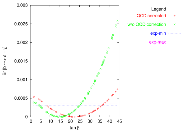
Refer to caption
Figure 3: Branching ratio as a function of tan⁑β𝛽\tan\!\beta in MSSM with Atsubscript𝐴𝑑A_{t} positive and ΞΌπœ‡\mu negative. The β€˜+’ sign is for the QCD corrected rate and the β€˜Γ—\times’ sign for the rate without QCD corrections. Two horizontal lines in this Fig. and all the following figures for branching fraction is the experimental uncertainty at 1​σ1𝜎1\sigma. See text for the values of various parameters.
Refer to caption
Figure 4: Various contributions to Wilson coefficients versus tan⁑β𝛽\tan\!\beta. SM (line with symbol β€˜+’) and charged Higgs (denoted as CS-L, line with β€˜*’ sign) are of the same sign (positive) whereas the chargino contribution (denoted as CH-L, line with ’x’ sign) has a strong tan⁑β𝛽\tan\!\beta dependence and is of opposite sign (negative) because At​μ<0subscriptπ΄π‘‘πœ‡0A_{t}\mu<0.
Refer to caption
Figure 5: Same as Fig.3, but with sign of ΞΌπœ‡\mu positive.

While investigating the influence of RPV we kept the spectrum similar to the one selected for the case of MSSM with sign of ΞΌπœ‡\mu negative and tan⁑β=37𝛽37\tan\!\beta=37. Note that in the large tan⁑β𝛽\tan\!\beta region QCD corrections drastically suppress the rate at the scale mbsubscriptπ‘šπ‘m_{b} (see for instance Fig.3). This is expected because, in the large tan⁑β𝛽\tan\!\beta region, the Wilson coefficient C7subscript𝐢7C_{7} is negative due to large negative chargino contribution and at the scale mbsubscriptπ‘šπ‘m_{b} after the QCD correction there is a destructive interference between C2subscript𝐢2C_{2} and C7subscript𝐢7C_{7}. The choice of spectrum is guided by requiring that in the MSSM limit we do obtain branching fraction well within experimental limits. Now the purpose is to investigate the behaviour of branching fraction once we turn on the knob of R𝑅R-parity violation. As we will see, both, enhancement as well as suppression is possible depending on which operator(s) are playing the major role. Both, the direct contribution, through the magnetic penguin, and the effect induced by QCD renormalization, through the various four-quark operators are significant.

Due to the large number of RPV parameters (48 just from the superpotential, with more from the soft SUSY breaking sector), without further knowledge of their plausible range of values it is impossible to extract any useful information on a phenomenological study, with all of them playing a role at the same time. Hence, the sensible thing to do at this stage is to focus on a minimal number at a time and study their possible impact. For the case at hand, a pair of parameters is taken at a time, while all the others are switched off. We discuss first the Ξ»β€²superscriptπœ†β€²\lambda^{\prime}-couplings. There are two possible combinations in which two non-zero Ξ»β€²superscriptπœ†β€²\lambda^{\prime} can give a finite contribution. These are (A) Ξ»i​3​j′​λh​2​kβˆ—β€²\lambda^{\prime}_{i3j}\lambda^{{}^{\prime}*}_{h2k} and (B) Ξ»i​j​3βˆ—β€²β€‹Ξ»h​k​2β€²\lambda^{{}^{\prime}*}_{ij3}\lambda^{{}^{\prime}}_{hk2}. We illustrate their effects in more detail below.

We will compare below the probable bounds we obtained with the similar bounds on the relevant combination of Ξ»β€²superscriptπœ†β€²\lambda^{\prime}-couplings in the literature. We have, first, to bring to the readers attention that the existing bounds in the literature are typically obtained assuming a sparticle spectrum of around 100 GeV. However, such a low lying spectrum is very dangerous for bβ†’s+γ→𝑏𝑠𝛾b\rightarrow s+\gammaΒ 444 To be exact, the top squarks contribute directly through the chargino diagram without the CKM suppression and have to be heavier. The bottom and strange squarks contribute, if their flavor violating mixings are nonzero. They are hence likely to be required to be heavier too. Otherwise, we can actually live with only heavier stops but a light sparticle here. Such a split in sparticle spectrum is considered unlikely as it goes in the opposite direction as predictions from most available SUSY breaking models. and quite unrealistic at least for the squarks. In consideration of that, and for a better comparison with the available bβ†’s+γ→𝑏𝑠𝛾b\rightarrow s+\gammaΒ result for the R𝑅R-conserving contributions (of the MSSM), we stick to a slightly heavier spectrum of 300 GeV squarks. Hence, the existing bounds must be rescaled by a factor of three for a better comparison with our bounds. Moreover, for some the combinations that contribute to bβ†’s+γ→𝑏𝑠𝛾b\rightarrow s+\gammaΒ there do not exist any direct bound. We have then made use of the best bounds available on the individual parameters to obtain a bound on such a combination.

V.0.1 Case A: Ξ»i​3​j′​λh​2​kβ€²β£βˆ—subscriptsuperscriptπœ†β€²π‘–3𝑗subscriptsuperscriptπœ†β€²β„Ž2π‘˜\lambda^{\prime}_{i3j}\lambda^{\prime*}_{h2k}

If the indices i,j,h,kπ‘–π‘—β„Žπ‘˜i,j,h,k are un-constrained, one can form 81 combinations of two Ξ»β€²superscriptπœ†β€²\lambda^{\prime}-couplings that can in principle contribute. However, in the limit there is no flavor off-diagonal mixing in the (s)neutrino mass matrix, the combination with iβ‰ hπ‘–β„Ži\neq h will not contribute. The case jβ‰ kπ‘—π‘˜j\neq k requires extra source of flavor off-diagonal squark mixing to contribute; hence is also not of interest here. So we shall confine ourselves to the case i=hπ‘–β„Ži=h and j=kπ‘—π‘˜j=k and hence study the impact of only nine (9) combinations, picking one of them to be non-zero at a given time. Note that so long as one sticks to the phenomenologically required suppression in all the flavor off-diagonal mass mixings from SUSY, the RPV contributions which require such mixings would be doubly suppressed and hence highly unlikely to be of any numerical significance. For the magnetic penguin operators, the contribution is of LL type.

The above combination will lead to a bRβ†’sLβ†’subscript𝑏𝑅subscript𝑠𝐿b_{\!\scriptscriptstyle R}\rightarrow s_{\!\scriptscriptstyle L} transition with mbsubscriptπ‘šπ‘m_{b} mass-insertion on external line. The contribution can come from chromo(magnetic) penguins (only sneutrino and neutrino loops are possible) or from the current-current operators 𝒬9,10,11subscript𝒬91011{\cal Q}_{9,10,11}. Sneutrino loops being proportional to the inverse of light slepton mass, are dominant compared to the neutrino loops which are suppressed by heavier squark mass. The important feature here is that the RPV contributions interfere with the SM and the MSSM contributions. Of the possible nine combinations, we will discuss three representative combinations with best bounds. The other six combinations follow similar pattern, as their contributions have a similar structure.

In our numerical analysis, we take real and equal values for two Ξ»β€²superscriptπœ†β€²\lambda^{\prime}-couplings at a time. As discussed above and illustrated by the analytical formulae, the contributions depend on the complex product. The strategy here then simplifies the results to one-parameter scenario for easy presentation, without compromising the physics. Consider the influence of the combinations |Ξ»13​k′​λ12​kβ€²|subscriptsuperscriptπœ†β€²13π‘˜subscriptsuperscriptπœ†β€²12π‘˜|\lambda^{\prime}_{13k}\lambda^{\prime}_{12k}|. For k=1,2π‘˜12k=1,2 the physics is identical because the relevant Wilson coefficients (C9,10subscript𝐢910C_{9,10}) have identical structure and so we shall discuss the combination |Ξ»132′​λ122β€²|subscriptsuperscriptπœ†β€²132subscriptsuperscriptπœ†β€²122|\lambda^{\prime}_{132}\lambda^{\prime}_{122}|. In Fig.6 we have plotted the branching ratio against Ξ»132β€²(=Ξ»122β€²)annotatedsubscriptsuperscriptπœ†β€²132absentsubscriptsuperscriptπœ†β€²122\lambda^{\prime}_{132}\;(=\lambda^{\prime}_{122}). Interestingly, the rate falls below the experimental limit (at Ξ»132β€²=Ξ»122β€²=0.07subscriptsuperscriptπœ†β€²132subscriptsuperscriptπœ†β€²1220.07\lambda^{\prime}_{132}=\lambda^{\prime}_{122}=0.07) with increasing Ξ»β€²superscriptπœ†β€²\lambda^{\prime} value, reaches a minimum and then rises again (the rise is not shown in the fig.). To understand this behavior we have plotted all the relevant Wilson coefficients against Ξ»β€²superscriptπœ†β€²\lambda^{\prime} values in Fig.7. It can be clearly seen that C7​(MW)subscript𝐢7subscriptπ‘€π‘ŠC_{7}(M_{\!\scriptscriptstyle W}) is falling with increasing Ξ»β€²superscriptπœ†β€²\lambda^{\prime} value. This is because of destructive interference between the negative R𝑅R-parity conserving contribution (sum of W-boson, charged Higgs and Chargino loop) and the positive sneutrino loop contribution, as seen in the figure. At the scale mbsubscriptπ‘šπ‘m_{b} after QCD running there is again destructive interference between the dominant tree level contribution from C10subscript𝐢10C_{10} and C7subscript𝐢7C_{7} [see eq. (IV)], because of which C7​(mb)subscript𝐢7subscriptπ‘šπ‘C_{7}(m_{b}) further falls with increasing Ξ»β€²superscriptπœ†β€²\lambda^{\prime} value. So because of these destructive interference, the branching ratio is falling below the experimental limit and we obtain a bound of |Ξ»132′​λ122β€²|<4.9Γ—10βˆ’3subscriptsuperscriptπœ†β€²132subscriptsuperscriptπœ†β€²1224.9superscript103|\lambda^{\prime}_{132}\lambda^{\prime}_{122}|<4.9\times 10^{-3}, to be compared with a rescaled existing bound of 3Γ—10βˆ’23superscript1023\times 10^{-2}.

Refer to caption
Figure 6: Branching fraction as a function of Ξ»132β€²(=Ξ»122β€²)annotatedsubscriptsuperscriptπœ†β€²132absentsubscriptsuperscriptπœ†β€²122\lambda^{\prime}_{132}\;(=\lambda^{\prime}_{122}).
Refer to caption
Figure 7: Wilson coefficients as a function of Ξ»132β€²(=Ξ»122β€²)annotatedsubscriptsuperscriptπœ†β€²132absentsubscriptsuperscriptπœ†β€²122\lambda^{\prime}_{132}\;(=\lambda^{\prime}_{122}). CH,CS,NS stand for the chargino, charged-Higgs and sneutrino contributions, respectively. The letter β€˜L’ indicates that these contributions go into C7subscript𝐢7C_{7}. Similar notation would apply to the following figures. The letter β€˜R’(L) would indicate that the contribution goes into coefficients with(without) tilde.
Refer to caption
Figure 8: Branching fraction as a function of Ξ»333β€²(=Ξ»323β€²)annotatedsubscriptsuperscriptπœ†β€²333absentsubscriptsuperscriptπœ†β€²323\lambda^{\prime}_{333}\;(=\lambda^{\prime}_{323}).
Refer to caption
Figure 9: Relevant Wilson coefficients as a function of Ξ»333β€²(=Ξ»323β€²)annotatedsubscriptsuperscriptπœ†β€²333absentsubscriptsuperscriptπœ†β€²323\lambda^{\prime}_{333}\;(=\lambda^{\prime}_{323}).

In Fig.8, we have plotted the branching ratio against Ξ»333β€²(=Ξ»323β€²)annotatedsubscriptsuperscriptπœ†β€²333absentsubscriptsuperscriptπœ†β€²323\lambda^{\prime}_{333}\;(=\lambda^{\prime}_{323}). Unlike the above case, here the relevant current-current Wilson coefficient C11subscript𝐢11C_{11} has a more important role to play. Not only does the scheme-independent effective coefficient C11effsuperscriptsubscript𝐢11effC_{11}^{\rm eff} influence C7​(mb)subscript𝐢7subscriptπ‘šπ‘C_{7}(m_{b}) through RG running, it also contributes to C7effsuperscriptsubscript𝐢7effC_{7}^{\rm eff} directly. The effect cancels with the R𝑅R-parity conserving contributions and hence C7eff​(MW)superscriptsubscript𝐢7effsubscriptπ‘€π‘ŠC_{7}^{\rm eff}(M_{\!\scriptscriptstyle W}) is seen to reduce with increasing Ξ»β€²superscriptπœ†β€²\lambda^{\prime} value. Even at the scale mbsubscriptπ‘šπ‘m_{b}, after QCD running there is a destructive interference between the R𝑅R-parity conserving and R𝑅R-parity violating parts and hence C7effsuperscriptsubscript𝐢7effC_{7}^{\rm eff} at mbsubscriptπ‘šπ‘m_{b} further reduces resulting in the branching fraction that falls with the RPV coupling. The fall is much stronger compared to the previous case. We obtain a bound of |Ξ»333′​λ323β€²|<1.6Γ—10βˆ’3subscriptsuperscriptπœ†β€²333subscriptsuperscriptπœ†β€²3231.6superscript103|\lambda^{\prime}_{333}\lambda^{\prime}_{323}|<1.6\times 10^{-3} to be compared with the rescaled existing bound of (1βˆ’3)Γ—10βˆ’213superscript102(1-3)\times 10^{-2} gautam .

V.0.2 Case B: Ξ»i​j​3βˆ—β€²β€‹Ξ»h​k​2β€²\lambda^{{}^{\prime}*}_{ij3}\lambda^{\prime}_{hk2}

Such a combination leads to a bLβ†’sRβ†’subscript𝑏𝐿subscript𝑠𝑅b_{\!\scriptscriptstyle L}\rightarrow s_{\!\scriptscriptstyle R} transition for mbsubscriptπ‘šπ‘m_{b} mass insertion on the external line. This would mean that the b𝑏b and s𝑠s quark at the effective vertices would be right handed. It contributes to the Wilson coefficients of several operators. These include the C~7,8subscript~𝐢78\widetilde{C}_{7,8} coefficients of the (chromo)magnetic penguins, via charged lepton, charged slepton, neutrino and sneutrino loop. Interestingly, in the SM and MSSM, this coefficient does not receive much contribution. The above combination can also contribute to Wilson coefficients of the current-current operators, 𝒬~9subscript~𝒬9{\widetilde{\cal Q}}_{9} to 𝒬~13subscript~𝒬13{\widetilde{\cal Q}}_{13}. These current-current contributions are mostly the dominant ones but not always as we will soon see.

As discussed at length in case (A), we must require i=hπ‘–β„Ži=h and j=kπ‘—π‘˜j=k and hence case (B) then effectively consists of the combinations Ξ»i​j​3β€²β£βˆ—β€‹Ξ»i​j​2β€²subscriptsuperscriptπœ†β€²π‘–π‘—3subscriptsuperscriptπœ†β€²π‘–π‘—2\lambda^{\prime*}_{ij3}\lambda^{\prime}_{ij2}. Consider Fig.10 where we have plotted the branching fraction against non-vanishing Ξ»233β€²(=Ξ»232β€²)annotatedsubscriptsuperscriptπœ†β€²233absentsubscriptsuperscriptπœ†β€²232\lambda^{\prime}_{233}\;(=\lambda^{\prime}_{232}). We get a bound |Ξ»233′​λ232β€²|<1.9Γ—10βˆ’2subscriptsuperscriptπœ†β€²233subscriptsuperscriptπœ†β€²2321.9superscript102|\lambda^{\prime}_{233}\lambda^{\prime}_{232}|<1.9\times 10^{-2}, to be compared with the rescaled existing bound of 4.4Γ—10βˆ’14.4superscript1014.4\times 10^{-1} gautam .

Refer to caption
Figure 10: Branching ratio as a function of Ξ»233β€²(=Ξ»232β€²)annotatedsubscriptsuperscriptπœ†β€²233absentsubscriptsuperscriptπœ†β€²232\lambda^{\prime}_{233}\;(=\lambda^{\prime}_{232}).
Refer to caption
Figure 11: Branching ratio as a function of Ξ»113β€²(=Ξ»112β€²)annotatedsubscriptsuperscriptπœ†β€²113absentsubscriptsuperscriptπœ†β€²112\lambda^{\prime}_{113}\;(=\lambda^{\prime}_{112}).

The mild behaviour of branching fraction suggests the existence of cancellations. In Fig.11 we have plotted branching fraction against Ξ»113β€²(=Ξ»112β€²)annotatedsubscriptsuperscriptπœ†β€²113absentsubscriptsuperscriptπœ†β€²112\lambda^{\prime}_{113}\;(=\lambda^{\prime}_{112}) and obtain a bound of |Ξ»113′​λ112β€²|<1.4Γ—10βˆ’2subscriptsuperscriptπœ†β€²113subscriptsuperscriptπœ†β€²1121.4superscript102|\lambda^{\prime}_{113}\lambda^{\prime}_{112}|<1.4\times 10^{-2}. Although the branching fraction behaves more or less similarly in both the above cases, the underlying dynamics is quite different. To better appreciate the differences, we have plotted the relevant Wilson coefficients in Fig.12 for the combination |Ξ»233′​λ232β€²|subscriptsuperscriptπœ†β€²233subscriptsuperscriptπœ†β€²232|\lambda^{\prime}_{233}\lambda^{\prime}_{232}| and in Fig.13 for the combination |Ξ»113′​λ112β€²|subscriptsuperscriptπœ†β€²113subscriptsuperscriptπœ†β€²112|\lambda^{\prime}_{113}\lambda^{\prime}_{112}|. In Fig.12, the horizontal line (circles) is the large R𝑅R-parity conserving contribution to C7​(mb)subscript𝐢7subscriptπ‘šπ‘C_{7}(m_{b}) which does not interfere with the RPV contributions going into C~7subscript~𝐢7\widetilde{C}_{7}. The surprising feature is the large (though less than R𝑅R-parity conserving contribution) positive contribution of C~7​(MW)subscript~𝐢7subscriptπ‘€π‘Š\widetilde{C}_{7}(M_{\!\scriptscriptstyle W}). This is surprising because it receives dominant negative sign contribution from the charged-slepton (crosses in the figure) whereas the positive sign sneutrino contribution (star marks in figure) is sub-dominant. Here again, the requirement of scheme-independence plays an important role because C~7eff​(ΞΌ)=C~7​(ΞΌ)βˆ’C~11​(ΞΌ)subscriptsuperscript~𝐢eff7πœ‡subscript~𝐢7πœ‡subscript~𝐢11πœ‡\widetilde{C}^{\rm eff}_{7}(\mu)=\widetilde{C}_{7}(\mu)-\widetilde{C}_{11}(\mu). It is the large negative sign contribution from C~11​(MW)subscript~𝐢11subscriptπ‘€π‘Š\widetilde{C}_{11}(M_{\!\scriptscriptstyle W}) which adds up with the positive sneutrino contribution and dictates the behaviour of C~7​(MW)subscript~𝐢7subscriptπ‘€π‘Š\widetilde{C}_{7}(M_{\!\scriptscriptstyle W}). At the scale mbsubscriptπ‘šπ‘m_{b} after QCD running, there is some suppression in the Wilson coefficient. Consider the case of the combination |Ξ»113′​λ112β€²|subscriptsuperscriptπœ†β€²113subscriptsuperscriptπœ†β€²112|\lambda^{\prime}_{113}\lambda^{\prime}_{112}| (see Fig.13). It has a peculiarity of the charged-scalar loop contribution slightly dominating the contribution from current-current Wilson coefficient C~9subscript~𝐢9\widetilde{C}_{9}. This suggests that it is not always true that tree-level contribution dominates. Such a dominance can be traced to two effects : (a) In contrast to the tree level contribution, a charged slepton loop contribution has contributions from two diagrams corresponding to photon being emitted from a charged slepton (∝proportional-to\propto to loop function F2subscript𝐹2F_{2}) and the photon being emitted from an up-type quark (∝F1proportional-toabsentsubscript𝐹1\propto F_{1}). (b) The values of loop functions depend on the mass of the quark in the loop – the lighter the quark less the suppression. Thus, provided that there is no CKM suppression, up-quark-charged-slepton loop dominates over the top-quark-charged-slepton loop and in fact can also dominate over the tree level contribution. That there is no CKM suppression in both the above cases can be easily verified from the formulae of the Wilson coefficients. Also the uniform dominance of charged slepton loop over sneutrino loop can be accounted for by the argument (a) above. Since there are two possible diagrams for charged slepton loop it brings in a charge factor of (2/3 + 1 = 5/3) which is five times bigger than the charge factor coming from the down-squark in the sneutrino loop. However, the charged-slepton and sneutrino loop contributions always come with opposite sign and hence there are cancellations.
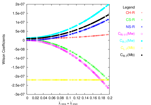
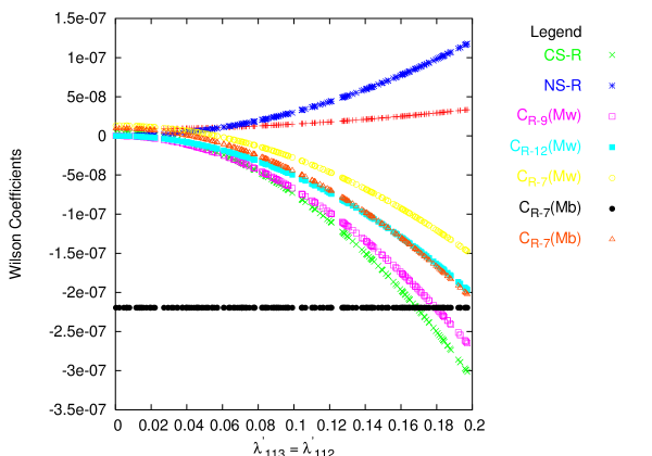
Refer to caption
Figure 12: Relevant Wilson coefficients as a function of Ξ»233β€²(=Ξ»232β€²)annotatedsubscriptsuperscriptπœ†β€²233absentsubscriptsuperscriptπœ†β€²232\lambda^{\prime}_{233}\;(=\lambda^{\prime}_{232}).
Refer to caption
Figure 13: Relevant Wilson coefficients as a function of Ξ»113β€²(=Ξ»112β€²)annotatedsubscriptsuperscriptπœ†β€²113absentsubscriptsuperscriptπœ†β€²112\lambda^{\prime}_{113}\;(=\lambda^{\prime}_{112}).
Table 1: Bounds on the various products of Ξ»β€²superscriptπœ†β€²\lambda^{\prime} obtained compared with the appropriately rescaled existing bounds gautam
Product |λ′​λ′|superscriptπœ†β€²superscriptπœ†β€²|\lambda^{\prime}\lambda^{\prime}| Our bound Existing bound Wilson coeff.
Case A
131.121 4.9Γ—10βˆ’34.9superscript1034.9\times 10^{-3} 2Γ—10βˆ’32superscript1032\times 10^{-3} C7,C9subscript𝐢7subscript𝐢9C_{7},C_{9}
132.122 4.9Γ—10βˆ’34.9superscript1034.9\times 10^{-3} 3Γ—10βˆ’23superscript1023\times 10^{-2} C7,C10subscript𝐢7subscript𝐢10C_{7},C_{10}
133.123 1.6Γ—10βˆ’31.6superscript1031.6\times 10^{-3} 7.2Γ—10βˆ’57.2superscript1057.2\times 10^{-5} C7,C11subscript𝐢7subscript𝐢11C_{7},C_{11}
231.221 4.9Γ—10βˆ’34.9superscript1034.9\times 10^{-3} 2Γ—10βˆ’22superscript1022\times 10^{-2} C7,C9subscript𝐢7subscript𝐢9C_{7},C_{9}
232.222 4.9Γ—10βˆ’34.9superscript1034.9\times 10^{-3} 2Γ—10βˆ’22superscript1022\times 10^{-2} C7,C10subscript𝐢7subscript𝐢10C_{7},C_{10}
233.223 1.6Γ—10βˆ’31.6superscript1031.6\times 10^{-3} 2Γ—10βˆ’22superscript1022\times 10^{-2} C7,C11subscript𝐢7subscript𝐢11C_{7},C_{11}
331.321 4.9Γ—10βˆ’34.9superscript1034.9\times 10^{-3} (1βˆ’3)Γ—10βˆ’213superscript102(1-3)\times 10^{-2} C7,C9subscript𝐢7subscript𝐢9C_{7},C_{9}
332.322 4.9Γ—10βˆ’34.9superscript1034.9\times 10^{-3} (1βˆ’3)Γ—10βˆ’213superscript102(1-3)\times 10^{-2} C7,C10subscript𝐢7subscript𝐢10C_{7},C_{10}
333.323 1.6Γ—10βˆ’31.6superscript1031.6\times 10^{-3} (1βˆ’3)Γ—10βˆ’213superscript102(1-3)\times 10^{-2} C7,C11subscript𝐢7subscript𝐢11C_{7},C_{11}
Case B
113.112 1.4Γ—10βˆ’21.4superscript1021.4\times 10^{-2} 1.3Γ—10βˆ’31.3superscript1031.3\times 10^{-3} C~7,C~9subscript~𝐢7subscript~𝐢9\widetilde{C}_{7},\widetilde{C}_{9}
123.122 1.4Γ—10βˆ’21.4superscript1021.4\times 10^{-2} 1.3Γ—10βˆ’31.3superscript1031.3\times 10^{-3} C~7,C~10subscript~𝐢7subscript~𝐢10\widetilde{C}_{7},\widetilde{C}_{10}
133.132 1.9Γ—10βˆ’21.9superscript1021.9\times 10^{-2} 7.2Γ—10βˆ’57.2superscript1057.2\times 10^{-5} C~7,C~11subscript~𝐢7subscript~𝐢11\widetilde{C}_{7},\widetilde{C}_{11}
213.212 1.4Γ—10βˆ’21.4superscript1021.4\times 10^{-2} 1.3Γ—10βˆ’31.3superscript1031.3\times 10^{-3} C~7,C~9subscript~𝐢7subscript~𝐢9\widetilde{C}_{7},\widetilde{C}_{9}
223.222 1.4Γ—10βˆ’21.4superscript1021.4\times 10^{-2} 1.3Γ—10βˆ’31.3superscript1031.3\times 10^{-3} C~7,C~10subscript~𝐢7subscript~𝐢10\widetilde{C}_{7},\widetilde{C}_{10}
233.232 1.9Γ—10βˆ’21.9superscript1021.9\times 10^{-2} 4.4Γ—10βˆ’14.4superscript1014.4\times 10^{-1} C~7,C~11subscript~𝐢7subscript~𝐢11\widetilde{C}_{7},\widetilde{C}_{11}
313.312 1.4Γ—10βˆ’21.4superscript1021.4\times 10^{-2} 1.3Γ—10βˆ’31.3superscript1031.3\times 10^{-3} C~7,C~9subscript~𝐢7subscript~𝐢9\widetilde{C}_{7},\widetilde{C}_{9}
323.322 1.4Γ—10βˆ’21.4superscript1021.4\times 10^{-2} 1.3Γ—10βˆ’31.3superscript1031.3\times 10^{-3} C~7,C~10subscript~𝐢7subscript~𝐢10\widetilde{C}_{7},\widetilde{C}_{10}
333.332 1.9Γ—10βˆ’21.9superscript1021.9\times 10^{-2} (1.3βˆ’9.2)Γ—10βˆ’11.39.2superscript101(1.3-9.2)\times 10^{-1} C~7,C~11subscript~𝐢7subscript~𝐢11\widetilde{C}_{7},{\widetilde{C}}_{11}

In Table1, we have listed bounds that we have obtained for the various Ξ»β€²superscriptπœ†β€²\lambda^{\prime}-coupling combinations among the cases (A) and (B). As far as one restricts oneself to the situation of two non-zero trilinear Ξ»β€²superscriptπœ†β€²\lambda^{\prime}-couplings, case (A) and case (B) are the only combinations that can contribute. With non-zero bilinears as well, or additional non-zero trilinears, there could be more combinations that can contribute. For instance one can have a combination of Ξ»i​3​j′​λh​k​2β€²subscriptsuperscriptπœ†β€²π‘–3𝑗subscriptsuperscriptπœ†β€²β„Žπ‘˜2\lambda^{\prime}_{i3j}\lambda^{\prime}_{hk2}, giving rise to a neutrino or a neutral scalar loop for the penguins. Since the overall process conserves lepton number, the above combination obviously needs to be supplemented with two more L-violating couplings. This could be from a Majorana mass-insertions for neutrino or sneutrino in the loop. However, such a contribution would be further suppressed and hence we skip presenting explicit results of the kind.

In all the above discussion, we have assumed that all the couplings are real and positive. It would be interesting to consider the possibility when there is a relative phase resulting in a relative negative sign among the chosen non-vanishing pair of Ξ»β€²superscriptπœ†β€²\lambda^{\prime} couplings. It turns out that such a case does not affect the bounds much. For the case (B) with dominant contributions from RPV couplings, it obviously cannot affect the decay rate which is modulus squared of Wilson coefficient. However for case (A), a negative or a positive sign can lead to constructive or destructive interference between R𝑅R-parity conserving and violating contributions. A relative negative sign though changes the sign of the slope for the branching fraction it does not alter its magnitude. Thus, the only implication as compared to the earlier bound which (for instance) was due to a branching fraction rising above the experimental limit, would now change to a bound due to the branching fraction falling below the experimental limit. The change in the magnitude of the bound is however nominal.

Finally, we comment briefly on contributions from Ξ»β€²β€²superscriptπœ†β€²β€²\lambda^{\prime\prime}-couplings. We obtain no useful bounds on the Ξ»β€²β€²superscriptπœ†β€²β€²\lambda^{\prime\prime}-couplings. The main reason behind this is that squark spectrum of 300 GeV is heavy enough to suppress the Ξ»β€²β€²superscriptπœ†β€²β€²\lambda^{\prime\prime} contributions. However, a lighter spectrum (although not viable due to large MSSM contributions) cannot lead to enhancement because of certain cancellations taking place. This provides a nice example of the interesting role played by the QCD running and hence worth a brief discussion. The combinations responsible for contributing to the decay rate can be written as: Ξ»h​n​3β€²β€²β£βˆ—β€‹Ξ»k​n​2β€²β€²subscriptsuperscriptπœ†β€²β€²β„Žπ‘›3subscriptsuperscriptπœ†β€²β€²π‘˜π‘›2\lambda^{\prime\prime*}_{hn3}\lambda^{\prime\prime}_{kn2} from the up-squark loop and Ξ»n​h​3β€²β€²β£βˆ—β€‹Ξ»n​k​2β€²β€²subscriptsuperscriptπœ†β€²β€²π‘›β„Ž3subscriptsuperscriptπœ†β€²β€²π‘›π‘˜2\lambda^{\prime\prime*}_{nh3}\lambda^{\prime\prime}_{nk2} from the down squark loop, thus contributing to C~7,8subscript~𝐢78{\widetilde{C}}_{7,8}. Depending on the particular value for the indices, there could also be contributions from the current-current operators with Wilson coefficients, C~1(=βˆ’C~2),C~14(=βˆ’C~15),C~16(=βˆ’C~17)annotatedsubscript~𝐢1absentsubscript~𝐢2annotatedsubscript~𝐢14absentsubscript~𝐢15annotatedsubscript~𝐢16absentsubscript~𝐢17{\widetilde{C}}_{1}(=-{\widetilde{C}}_{2}),{\widetilde{C}}_{14}(=-{\widetilde{C}}_{15}),{\widetilde{C}}_{16}(=-{\widetilde{C}}_{17}). It might appear that the relative negative signs for the above coefficients leads to cancellations and hence there is no impact on the decay rate. This is not what is happening. There are cancellations, but these result rather from the form of C~7subscript~𝐢7{\widetilde{C}}_{7} at the scale (mb)subscriptπ‘šπ‘(m_{b}) (see eq.(IV). Taking into account, the antisymmetry in the last two indices, one can form 18 combinations from the above mentioned general form of the Ξ»β€²β€²superscriptπœ†β€²β€²\lambda^{\prime\prime} contributions (12 combinations contributing to the down-squark loop and 9 to the up-squark loop but 3 three combinations common to both). There are two reasons that kill the contributions. In a few cases, the loop level contribution is accompanied by current-current Wilson coefficients pairs C~14subscript~𝐢14{\widetilde{C}}_{14} and C~16subscript~𝐢16{\widetilde{C}}_{16}, or C~1subscript~𝐢1{\widetilde{C}}_{1} and C~16subscript~𝐢16{\widetilde{C}}_{16}. Although these pairs contribute about equal magnitude with identical sign, at the scale mbsubscriptπ‘šπ‘m_{b} after QCD running these are multiplied by about equal coefficients but with opposite sign and hence the cancellations. The rest of the combinations get contributions from only one among the above pairs and hence cannot suffer from above cancellations. In this case, they all require flavor violating mass-insertions for (s)particles in the loop. The only exception to above two cases is the combination Ξ»313β€²β€²β£βˆ—β€‹Ξ»212β€²β€²subscriptsuperscriptπœ†β€²β€²313subscriptsuperscriptπœ†β€²β€²212\lambda^{\prime\prime*}_{\scriptscriptstyle 313}\lambda^{\prime\prime}_{\scriptscriptstyle 212} for which we get a bound of 0.5. This bound is very weak when compared to existing bound from other sources( 6.2Γ—10βˆ’36.2superscript1036.2\times 10^{-3}gautam ).

VI Conclusion

In summary, we present a complete analysis of the decay rate bβ†’s+γ→𝑏𝑠𝛾b\rightarrow s+\gammaΒ at the leading log order for the generic supersymmetric SM, or SUSY without R𝑅R-parity. Unlike previous studies on the topic, our results are fully generic, admitting all possible forms of R𝑅R-parity violation without a priori assumption. We use exact mass eigenstates in our formulae, hence free from the otherwise commonly used mass-insertion approximation. In case one prefers, our formulation does provide perturbative approximations through which the explicit dependence on all RPV parameters can be extracted otto-gssm . We consider the analytical results useful for any detailed study on the model in relation to the radiative B decay.

In the numerical implementation of the analytical formulas our focus, is on the Ξ»β€²superscriptπœ†β€²\lambda^{\prime} couplings. For simplicity and feasibility, we keep two non-vanishing Ξ»β€²superscriptπœ†β€²\lambda^{\prime}-couplings. The choice of the mass spectrum and various parameters of the model is dictated by the requirement that in the limit of R𝑅R-parity conserving SUSY, the branching ratio falls within the experimental limits. Then, switching on the non-zero values of the (combination of two) Ξ»β€²superscriptπœ†β€²\lambda^{\prime}-couplings allows us to trace their contribution and obtain bounds on the class of RPV parameters from imposing the experimental constraints. In this aspect, the strategy is common to many of the earlier studies. We find that RPV contributions not only expand the relevant four-quark operator basis of the case of MSSM from 8 to 28, but also introduce new, likely to be dominating, contributions in the form of charged-slepton and sneutrino loops to the Wilson coefficients of (chromo)magnetic penguins. However, our results clearly show that the new four-quark operators with non-vanishing Wilson coefficients at the electroweak/SUSY scale, induce effects through QCD running which typically dominate over the direct contributions to the Wilson coefficients of (chromo)magnetic penguins. However, there are exceptions. Depending on the particles exchanged, the loop contributions could also dominate in some cases.

The two-Ξ»β€²superscriptπœ†β€²\lambda^{\prime} type of RPV contributions split into two classes: (A) Ξ»i​3​j′​λh​2​kβ€²β£βˆ—subscriptsuperscriptπœ†β€²π‘–3𝑗subscriptsuperscriptπœ†β€²β„Ž2π‘˜\lambda^{\prime}_{i3j}\lambda^{\prime*}_{h2k} and (B) Ξ»i​j​3β€²β£βˆ—β€‹Ξ»h​k​2β€²subscriptsuperscriptπœ†β€²π‘–π‘—3subscriptsuperscriptπœ†β€²β„Žπ‘˜2\lambda^{\prime*}_{ij3}\lambda^{\prime}_{hk2}. Whereas the contributions in class (A) give rise to bRβ†’sLβ†’subscript𝑏𝑅subscript𝑠𝐿b_{\!\scriptscriptstyle R}\rightarrow s_{\!\scriptscriptstyle L} transition and hence in direct interference with major contributions from SM and R𝑅R-parity conserving SUSY parts, the contributions in class (B) have not much R𝑅R-parity conserving counterparts. We obtain numerical bounds, some cases of which are orders of magnitude stronger than available bounds in the literature. The interpretation of such bounds has to be taken more carefully. Their values depend strongly on the choice of other SUSY parameters. Moreover, it could happen that the R𝑅R-parity conserving and RPV contributions have some accidental, but strong cancellation. In the latter case, no meaningful bounds on the RPV couplings alone can be obtained. After all, the extra contributions in the case of MSSM are expected to have partial cancellations to offset the strong charged Higgs contribution. Our numerical results at least indicate clearly the strong implication of RPV couplings on bβ†’s+γ→𝑏𝑠𝛾b\rightarrow s+\gammaΒ at a level substantially beyond earlier studies are able to illustrate. A most conservative interpretation of the bounds obtained would be that they indicate values of the Ξ»β€²superscriptπœ†β€²\lambda^{\prime}-couplings around and above which the corresponding RPV contribution alone to bβ†’s+γ→𝑏𝑠𝛾b\rightarrow s+\gammaΒ  would be of alarming magnitude. We also explain clearly why the Ξ»β€²β€²superscriptπœ†β€²β€²\lambda^{\prime\prime}-couplings have no major role to play in bβ†’s+γ→𝑏𝑠𝛾b\rightarrow s+\gamma. Another type of significant contributions come from combinations of a bilinear and a trilinear RPV couplings. The type of contributions has a quite different structure and has not been studied before. They are implicitly included in our comprehensive formulation presented here, while the relevant numerical study is to be presented in another publication017 .

All the discussions above, like most of the earlier studies, has not taken into consideration constraints on the RPV parameters from the neutrino masses. However, taking the reasonable assumption that all the neutrino masses are in the sub-eV range, and that there are no strong cancellations among RPV contributions, very stringent constraints on the parameters can be obtained kong-neutrino ; kong-kang ; rv-tri ; cheung-kong . In fact, such constraints are so important that talking about other numerical constraints on RPV parameters without reference to the neutrino mass constraints may not be a sensible way to take the model seriously. So, we would like to comment on the issue here. Majorana neutrino masses could be induced at one loop level by a pair of trilinear RPV couplings Ξ»i​l​m′​λj​m​lβ€²subscriptsuperscriptπœ†β€²π‘–π‘™π‘šsubscriptsuperscriptπœ†β€²π‘—π‘šπ‘™\lambda^{\prime}_{ilm}\lambda^{\prime}_{jml}. Because these violate lepton number by two units, they cannot contribute to the decay bβ†’s+γ→𝑏𝑠𝛾b\rightarrow s+\gammaΒ . However, the case l=mπ‘™π‘šl=m could be used to obtain bounds on Ξ»i​m​mβ€²subscriptsuperscriptπœ†β€²π‘–π‘šπ‘š\lambda^{\prime}_{imm}. Strong bounds on such individual couplings could significantly strengthen the bounds on some of the combinations that contribute to bβ†’s+γ→𝑏𝑠𝛾b\rightarrow s+\gammaΒ . For instance, choosing the spectrum similar to the one for this study, one obtains a strong upper bound of |Ξ»i​33β€²|=7.1Γ—10βˆ’4subscriptsuperscriptπœ†β€²π‘–337.1superscript104|\lambda^{\prime}_{i33}|=7.1\times 10^{-4}. The bound on the parameter Ξ»i​22β€²subscriptsuperscriptπœ†β€²π‘–22\lambda^{\prime}_{i22} is much less stringent (|Ξ»i​22β€²|=3.0Γ—10βˆ’2subscriptsuperscriptπœ†β€²π‘–223.0superscript102|\lambda^{\prime}_{i22}|=3.0\times 10^{-2}) as it is suppressed by a quadratic factor of (ms/mb)2superscriptsubscriptπ‘šπ‘ subscriptπ‘šπ‘2(m_{s}/m_{b})^{2} relative to the one-loop contribution from the parameter Ξ»i​33β€²subscriptsuperscriptπœ†β€²π‘–33\lambda^{\prime}_{i33}. This would mean that, whenever the coupling Ξ»i​m​mβ€²subscriptsuperscriptπœ†β€²π‘–π‘šπ‘š\lambda^{\prime}_{imm} is a part of the combination contributing to bβ†’s+γ→𝑏𝑠𝛾b\rightarrow s+\gammaΒ , bounds coming from neutrino mass consideration are stronger. Nevertheless, the bounds obtained by us on three combinations in case (B), namely |Ξ»131′​λ121β€²|,|Ξ»231′​λ221β€²|,|Ξ»331′​λ321β€²|subscriptsuperscriptπœ†β€²131subscriptsuperscriptπœ†β€²121subscriptsuperscriptπœ†β€²231subscriptsuperscriptπœ†β€²221subscriptsuperscriptπœ†β€²331subscriptsuperscriptπœ†β€²321|\lambda^{\prime}_{131}\lambda^{\prime}_{121}|,|\lambda^{\prime}_{231}\lambda^{\prime}_{221}|,|\lambda^{\prime}_{331}\lambda^{\prime}_{321}|, still survive because Ξ»i​m​mβ€²subscriptsuperscriptπœ†β€²π‘–π‘šπ‘š\lambda^{\prime}_{imm} does not figure in these combinations.

note added in proof: Just after this work was finished, an eprint neubert-new appeared, where the branching fraction for Bβ†’Xs+γ→𝐡subscript𝑋𝑠𝛾B\rightarrow X_{s}+\gammaΒ has been recalculated at the NLL order using the results of soft-collinear factorization for inclusive B𝐡B-meson decay distributions. It has been pointed out that the singnificant perturbative uncertainties associated with the parameter Ξ”=mbβˆ’2​E0Ξ”subscriptπ‘šπ‘2subscript𝐸0\Delta=m_{b}-2E_{0} have been ignored in the previous works. The new estimate now stands at B​r​[Bβ†’Xs+γ​(EΞ³>1.8​G​e​V)]SM=(3.44Β±0.53Β±0.35)Γ—10βˆ’4π΅π‘Ÿsubscriptdelimited-[]→𝐡subscript𝑋𝑠𝛾subscript𝐸𝛾1.8𝐺𝑒𝑉SMplus-or-minus3.440.530.35superscript104Br\left[B\rightarrow X_{s}+\gamma\;(E_{\gamma}>1.8GeV)\right]_{\scriptscriptstyle\mathrm{SM}}=(3.44\pm 0.53\pm 0.35)\times 10^{-4}, where the first error is the estimate of perturbative uncertainties and the second one reflects uncertainties in the input parameters. As a result of this larger theoretical uncertainties, the lower bound on the charged-Higgs mass is strongly reduced compared to previous estimates, to slightly below 200 GeV at 95 % confidence level. With the larger theoretical uncertainties in the SM prediction, the case for new physics certainly becomes stronger.

Acknowledgment: O.K. thanks the Institute of Physics, Academia Sinica, Taiwan for hospitality during the early phase of the work. R.V. acknowledges the hospitality of the Korea Institute for Advanced Study (KIAS), Korea and KEK, Japan, during his visit where a part of the manuscript was written. We also thank E.J.Chun, H.-N.Li, K. Hagiwara and K.S.Babu for the useful discussions and N.Oshimo for the correspondence. Our work is partially supported by research grants from the National Science Council of Taiwan. O.K. is supported under grant number NSC 92-2112-M-008-044 and NSC 91-2112-M-008-042. R.V. is supported under post-doc grant number NSC 92-2811-M-008-012 and NSC 92-2811-M-008-003.

Appendix A The γ𝛾\gamma matrix

In table 2,3 we provide a translation of our notation of operators to that of refs.besmer ; chun-bsg for easy comparison. We define the scheme independent anomalous dimension matrix Ξ³^effsuperscript^𝛾eff{\hat{\gamma}}^{{\rm eff}} as:

Ξ³^(0)​eff=(Ξ³Leff00Ξ³Reff)superscript^𝛾0effsuperscriptsubscript𝛾𝐿eff00superscriptsubscript𝛾𝑅eff{\hat{\gamma}}^{{(0)\rm eff}}=\left(\begin{array}[]{cc}\gamma_{\!\scriptscriptstyle L}^{\rm eff}&0\\ 0&\gamma_{\!\scriptscriptstyle R}^{\rm eff}\\ \end{array}\right) (72)

where Ξ³Leffsuperscriptsubscript𝛾𝐿eff\gamma_{\!\scriptscriptstyle L}^{\rm eff} and Ξ³Reffsuperscriptsubscript𝛾𝑅eff\gamma_{\!\scriptscriptstyle R}^{\rm eff} are given as (for convenience we have given the operators on the top row):

Ξ³Leff=𝒬1𝒬2𝒬3𝒬4𝒬5𝒬6𝒬7𝒬8𝒬9𝒬10𝒬11(βˆ’260000030006βˆ’2βˆ’2923βˆ’292341681702700000βˆ’229223βˆ’4943βˆ’46481545270000044943βˆ’109103136815122700000002βˆ’6329βˆ’59300000βˆ’109103βˆ’109βˆ’383βˆ’29681βˆ’703270000000003230000000000βˆ’32928300000βˆ’2923βˆ’292320081βˆ’11927βˆ’160000βˆ’2923βˆ’292320081βˆ’119270βˆ’16000βˆ’2923βˆ’292320081βˆ’2272700βˆ’16)superscriptsubscript𝛾𝐿effsubscript𝒬1subscript𝒬2subscript𝒬3subscript𝒬4subscript𝒬5subscript𝒬6subscript𝒬7subscript𝒬8subscript𝒬9subscript𝒬10subscript𝒬112600000300062292329234168170270000022922349434648154527000004494310910313681512270000000263295930000010910310938329681703270000000003230000000000329283000002923292320081119271600002923292320081119270160002923292320081227270016\gamma_{\!\scriptscriptstyle L}^{\rm eff}=\begin{array}[]{c}\begin{array}[]{rrrrrrrrrrr}{\cal Q}_{1}&\;{\cal Q}_{2}&\;{\cal Q}_{3}&\;{\cal Q}_{4}&\;{\cal Q}_{5}&\;{\cal Q}_{6}&\;\;{\cal Q}_{7}&\;\;{\cal Q}_{8}&\;\,{\cal Q}_{9}&\;\,{\cal Q}_{10}&\;\,{\cal Q}_{11}\end{array}\\ \left(\begin{array}[]{rrrrrrrrrrr}-2&6&0&0&0&0&0&3&0&0&0\\ 6&-2&-\frac{2}{9}&\frac{2}{3}&-\frac{2}{9}&\frac{2}{3}&\frac{416}{81}&\frac{70}{27}&0&0&0\\ 0&0&-\frac{22}{9}&\frac{22}{3}&-\frac{4}{9}&\frac{4}{3}&-\frac{464}{81}&\frac{545}{27}&0&0&0\\ 0&0&\frac{44}{9}&\frac{4}{3}&-\frac{10}{9}&\frac{10}{3}&\frac{136}{81}&\frac{512}{27}&0&0&0\\ 0&0&0&0&2&-6&\frac{32}{9}&\frac{-59}{3}&0&0&0\\ 0&0&-\frac{10}{9}&\frac{10}{3}&-\frac{10}{9}&-\frac{38}{3}&-\frac{296}{81}&-\frac{703}{27}&0&0&0\\ 0&0&0&0&0&0&\frac{32}{3}&0&0&0&0\\ 0&0&0&0&0&0&-\frac{32}{9}&\frac{28}{3}&0&0&0\\ 0&0&-\frac{2}{9}&\frac{2}{3}&-\frac{2}{9}&\frac{2}{3}&\frac{200}{81}&-\frac{119}{27}&-16&0&0\\ 0&0&-\frac{2}{9}&\frac{2}{3}&-\frac{2}{9}&\frac{2}{3}&\frac{200}{81}&-\frac{119}{27}&0&-16&0\\ 0&0&-\frac{2}{9}&\frac{2}{3}&-\frac{2}{9}&\frac{2}{3}&\frac{200}{81}&-\frac{227}{27}&0&0&-16\\ \end{array}\right)\end{array} (73)
Ξ³Reff=𝒬~1𝒬~2𝒬~3𝒬~4𝒬~5𝒬~6𝒬~7𝒬~8𝒬~9𝒬~10𝒬~11𝒬~12𝒬~13𝒬~14𝒬~15𝒬~16𝒬~17(βˆ’260000030000000006βˆ’2βˆ’2923βˆ’292341681702700000000000βˆ’229223βˆ’4943βˆ’46481545270000000000044943βˆ’109103136815122700000000000002βˆ’6399βˆ’59300000000000βˆ’109103βˆ’109βˆ’383βˆ’29681βˆ’703270000000000000003230000000000000000βˆ’32928300000000000βˆ’2923βˆ’292320081βˆ’11927βˆ’160000000000βˆ’2923βˆ’292320081βˆ’119270βˆ’16000000000βˆ’2923βˆ’292320081βˆ’2272700βˆ’1600000000βˆ’2923βˆ’2923βˆ’44881βˆ’11927000βˆ’160000000βˆ’2923βˆ’2923βˆ’44881βˆ’119270000βˆ’1600000000000300000βˆ’260000βˆ’2923βˆ’2923416817027000006βˆ’200000000030000000βˆ’2600βˆ’2923βˆ’2923βˆ’23281702700000006βˆ’2)superscriptsubscript𝛾𝑅effsubscript~𝒬1subscript~𝒬2subscript~𝒬3subscript~𝒬4subscript~𝒬5subscript~𝒬6subscript~𝒬7subscript~𝒬8subscript~𝒬9subscript~𝒬10subscript~𝒬11subscript~𝒬12subscript~𝒬13subscript~𝒬14subscript~𝒬15subscript~𝒬16subscript~𝒬172600000300000000062292329234168170270000000000022922349434648154527000000000004494310910313681512270000000000000263995930000000000010910310938329681703270000000000000003230000000000000000329283000000000002923292320081119271600000000002923292320081119270160000000002923292320081227270016000000002923292344881119270001600000002923292344881119270000160000000000030000026000029232923416817027000006200000000030000000260029232923232817027000000062\displaystyle\gamma_{\!\scriptscriptstyle R}^{\rm eff}=\begin{array}[]{c}\begin{array}[]{rrrrrrrrrrrrrrrrr}\;\;\,{{\widetilde{\cal Q}}_{1}}&\,{{\widetilde{\cal Q}}_{2}}&\;\,{{\widetilde{\cal Q}}_{3}}&{{\widetilde{\cal Q}}_{4}}&\;\,{{\widetilde{\cal Q}}_{5}}&\;\;{{\widetilde{\cal Q}}_{6}}&\,\,\;\;{{\widetilde{\cal Q}}_{7}}&\,\;\;\,{{\widetilde{\cal Q}}_{8}}&\;{{\widetilde{\cal Q}}_{9}}&\,{{\widetilde{\cal Q}}_{10}}&\,{{\widetilde{\cal Q}}_{11}}&\,{{\widetilde{\cal Q}}_{12}}&\,{{\widetilde{\cal Q}}_{13}}&{{\widetilde{\cal Q}}_{14}}&\!{{\widetilde{\cal Q}}_{15}}&\!{{\widetilde{\cal Q}}_{16}}&\!{{\widetilde{\cal Q}}_{17}}\end{array}\\ \left(\begin{array}[]{rrrrrrrrrrrrrrrrr}-2&6&0&0&0&0&0&3&0&0&0&0&0&0&0&0&0\\ 6&-2&-\frac{2}{9}&\frac{2}{3}&-\frac{2}{9}&\frac{2}{3}&\frac{416}{81}&\frac{70}{27}&0&0&0&0&0&0&0&0&0\\ 0&0&-\frac{22}{9}&\frac{22}{3}&-\frac{4}{9}&\frac{4}{3}&-\frac{464}{81}&\frac{545}{27}&0&0&0&0&0&0&0&0&0\\ 0&0&\frac{44}{9}&\frac{4}{3}&-\frac{10}{9}&\frac{10}{3}&\frac{136}{81}&\frac{512}{27}&0&0&0&0&0&0&0&0&0\\ 0&0&0&0&2&-6&\frac{39}{9}&-\frac{59}{3}&0&0&0&0&0&0&0&0&0\\ 0&0&-\frac{10}{9}&\frac{10}{3}&-\frac{10}{9}&-\frac{38}{3}&-\frac{296}{81}&-\frac{703}{27}&0&0&0&0&0&0&0&0&0\\ 0&0&0&0&0&0&\frac{32}{3}&0&0&0&0&0&0&0&0&0&0\\ 0&0&0&0&0&0&-\frac{32}{9}&\frac{28}{3}&0&0&0&0&0&0&0&0&0\\ 0&0&-\frac{2}{9}&\frac{2}{3}&-\frac{2}{9}&\frac{2}{3}&\frac{200}{81}&-\frac{119}{27}&-16&0&0&0&0&0&0&0&0\\ 0&0&-\frac{2}{9}&\frac{2}{3}&-\frac{2}{9}&\frac{2}{3}&\frac{200}{81}&-\frac{119}{27}&0&-16&0&0&0&0&0&0&0\\ 0&0&-\frac{2}{9}&\frac{2}{3}&-\frac{2}{9}&\frac{2}{3}&\frac{200}{81}&-\frac{227}{27}&0&0&-16&0&0&0&0&0&0\\ 0&0&-\frac{2}{9}&\frac{2}{3}&-\frac{2}{9}&\frac{2}{3}&-\frac{448}{81}&-\frac{119}{27}&0&0&0&-16&0&0&0&0&0\\ 0&0&-\frac{2}{9}&\frac{2}{3}&-\frac{2}{9}&\frac{2}{3}&-\frac{448}{81}&-\frac{119}{27}&0&0&0&0&-16&0&0&0&0\\ 0&0&0&0&0&0&0&3&0&0&0&0&0&-2&6&0&0\\ 0&0&-\frac{2}{9}&\frac{2}{3}&-\frac{2}{9}&\frac{2}{3}&\frac{416}{81}&\frac{70}{27}&0&0&0&0&0&6&-2&0&0\\ 0&0&0&0&0&0&0&3&0&0&0&0&0&0&0&-2&6\\ 0&0&-\frac{2}{9}&\frac{2}{3}&-\frac{2}{9}&\frac{2}{3}&-\frac{232}{81}&\frac{70}{27}&0&0&0&0&0&0&0&6&-2\\ \end{array}\right)\end{array} (94)
(95)
Table 2: Operators that mix in the block Ξ³Leffsuperscriptsubscript𝛾𝐿eff\gamma_{\!\scriptscriptstyle L}^{\rm eff}
Our notation 𝒬1subscript𝒬1{\cal Q}_{1} 𝒬2subscript𝒬2{\cal Q}_{2} 𝒬3subscript𝒬3{\cal Q}_{3} 𝒬4subscript𝒬4{\cal Q}_{4} 𝒬5subscript𝒬5{\cal Q}_{5} 𝒬6subscript𝒬6{\cal Q}_{6} 𝒬7subscript𝒬7{\cal Q}_{7} 𝒬8subscript𝒬8{\cal Q}_{8} 𝒬9subscript𝒬9{\cal Q}_{9} 𝒬10subscript𝒬10{\cal Q}_{10} 𝒬11subscript𝒬11{\cal Q}_{11}
Ref.chun-bsg O1​Lsubscript𝑂1𝐿O_{\!\scriptscriptstyle 1L} O2​Lsubscript𝑂2𝐿O_{\!\scriptscriptstyle 2L} O3​Lsubscript𝑂3𝐿O_{\!\scriptscriptstyle 3L} O4​Lsubscript𝑂4𝐿O_{\!\scriptscriptstyle 4L} O5​Lsubscript𝑂5𝐿O_{\!\scriptscriptstyle 5L} O6​Lsubscript𝑂6𝐿O_{\!\scriptscriptstyle 6L} O7​Lsubscript𝑂7𝐿O_{\!\scriptscriptstyle 7L} O8​Lsubscript𝑂8𝐿O_{\!\scriptscriptstyle 8L} O6​Ldsubscriptsuperscript𝑂𝑑6𝐿O^{d}_{\!\scriptscriptstyle 6L} O6​Lssubscriptsuperscript𝑂𝑠6𝐿O^{s}_{\!\scriptscriptstyle 6L} O6​Lbsubscriptsuperscript𝑂𝑏6𝐿O^{b}_{\!\scriptscriptstyle 6L}
Ref.besmer O1subscript𝑂1O_{1} O2subscript𝑂2O_{2} O3subscript𝑂3O_{3} O4subscript𝑂4O_{4} O5subscript𝑂5O_{5} O6subscript𝑂6O_{6} O7subscript𝑂7O_{7} O8subscript𝑂8O_{8} P6subscript𝑃6P_{\scriptscriptstyle 6} P7subscript𝑃7P_{\scriptscriptstyle 7} P8subscript𝑃8P_{\scriptscriptstyle 8}
Table 3: Operators that mix in the block Ξ³Reffsuperscriptsubscript𝛾𝑅eff\gamma_{\!\scriptscriptstyle R}^{\rm eff} .
Our notation 𝒬~1subscript~𝒬1{{\widetilde{\cal Q}}_{1}} 𝒬~2subscript~𝒬2{{\widetilde{\cal Q}}_{2}} 𝒬~3subscript~𝒬3{{\widetilde{\cal Q}}_{3}} 𝒬~4subscript~𝒬4{{\widetilde{\cal Q}}_{4}} 𝒬~5subscript~𝒬5{{\widetilde{\cal Q}}_{5}} 𝒬~6subscript~𝒬6{{\widetilde{\cal Q}}_{6}} 𝒬~7subscript~𝒬7{{\widetilde{\cal Q}}_{7}} 𝒬~8subscript~𝒬8{{\widetilde{\cal Q}}_{8}} 𝒬~9subscript~𝒬9{{\widetilde{\cal Q}}_{9}} 𝒬~10subscript~𝒬10{{\widetilde{\cal Q}}_{10}} 𝒬~11subscript~𝒬11{{\widetilde{\cal Q}}_{11}} 𝒬~12subscript~𝒬12{{\widetilde{\cal Q}}_{12}} 𝒬~13subscript~𝒬13{{\widetilde{\cal Q}}_{13}} 𝒬~14subscript~𝒬14{{\widetilde{\cal Q}}_{14}} 𝒬~15subscript~𝒬15{{\widetilde{\cal Q}}_{15}} 𝒬~16subscript~𝒬16{{\widetilde{\cal Q}}_{16}} 𝒬~17subscript~𝒬17{{\widetilde{\cal Q}}_{17}}
Ref.chun-bsg O1​Rsubscript𝑂1𝑅O_{\!\scriptscriptstyle 1R} O2​Rsubscript𝑂2𝑅O_{\!\scriptscriptstyle 2R} O3​Rsubscript𝑂3𝑅O_{\!\scriptscriptstyle 3R} O4​Rsubscript𝑂4𝑅O_{\!\scriptscriptstyle 4R} O5​Rsubscript𝑂5𝑅O_{\!\scriptscriptstyle 5R} O6​Rsubscript𝑂6𝑅O_{\!\scriptscriptstyle 6R} O7​Rsubscript𝑂7𝑅O_{\!\scriptscriptstyle 7R} O8​Rsubscript𝑂8𝑅O_{\!\scriptscriptstyle 8R} O6​Rdsubscriptsuperscript𝑂𝑑6𝑅O^{d}_{\!\scriptscriptstyle 6R} O6​Rssubscriptsuperscript𝑂𝑠6𝑅O^{s}_{\!\scriptscriptstyle 6R} O6​Rbsubscriptsuperscript𝑂𝑏6𝑅O^{b}_{\!\scriptscriptstyle 6R} O6​Rusubscriptsuperscript𝑂𝑒6𝑅O^{u}_{\!\scriptscriptstyle 6R} O6​Rcsubscriptsuperscript𝑂𝑐6𝑅O^{c}_{\!\scriptscriptstyle 6R} O3​Rusubscriptsuperscript𝑂𝑒3𝑅O^{u}_{\!\scriptscriptstyle 3R} O4​Rusubscriptsuperscript𝑂𝑒4𝑅O^{u}_{\!\scriptscriptstyle 4R} O3​Rdsubscriptsuperscript𝑂𝑑3𝑅O^{d}_{\!\scriptscriptstyle 3R} O4​Rdsubscriptsuperscript𝑂𝑑4𝑅O^{d}_{\!\scriptscriptstyle 4R}
Ref.besmer R3subscript𝑅3R_{\scriptscriptstyle 3} R4subscript𝑅4R_{\!\scriptscriptstyle 4} P9subscript𝑃9P_{\scriptscriptstyle 9} P10subscript𝑃10P_{\scriptscriptstyle 10} P11subscript𝑃11P_{\scriptscriptstyle 11} P12subscript𝑃12P_{\scriptscriptstyle 12} O~7subscript~𝑂7{\widetilde{O}}_{7} O~8subscript~𝑂8{\widetilde{O}}_{8} P3subscript𝑃3P_{\scriptscriptstyle 3} P4subscript𝑃4P_{\scriptscriptstyle 4} P5subscript𝑃5P_{\scriptscriptstyle 5} P1subscript𝑃1P_{\scriptscriptstyle 1} P2subscript𝑃2P_{\scriptscriptstyle 2} R1subscript𝑅1R_{\scriptscriptstyle 1} R2subscript𝑅2R_{\scriptscriptstyle 2} R5subscript𝑅5R_{\scriptscriptstyle 5} R6subscript𝑅6R_{\scriptscriptstyle 6}

References

  • (1) K. Hagiwara et.al. [Particle Data Group Collaboration], β€œReview of Particle Physics,” Phys. Rev. D 66 010001 (2002).
  • (2) For the earlier works, see B.Grinstein et al.Β  Phys. Lett. B202 138 (1988); R.Grigjanis et al.Β  Phys. Lett. B213 355 (1988); M.Misiak Phys. Lett. B269 161 (1991), Nucl. Phys. B393 23 (1993); The issue of β€˜scheme dependence’ was resolved by M.Ciuchini et al.Β  Phys. Lett. B316 127 (1993), Nucl. Phys. B421 41 (1994).
  • (3) Scheme-independence was further confirmed using an unconventional scheme by G. Cella et al.Β  Nucl. Phys. B421 417 (1994), Phys. Lett. B325 227 (1994).
  • (4) P. Gambino and M. Misiak Nucl. Phys. B611 01 (20338). Also see A. Kagan and M. Neubert Eur. Phys. J.C 7 5 (1999).
  • (5) A. Buras et al.Β  Nucl. Phys. B631 219 (2002).
  • (6) S. Chen et al.Β (CLEO Collaboration) Phys. Rev. Lett. 87 251807 (2001).
  • (7) K. Abe et al.(BELLE Collaboration) Phys. Lett. B511 151 (2001).
  • (8) R. Barate et al.Β (ALEPH Collaboration) Phys. Lett. B429 169 (1998).
  • (9) C. Jessop, SLAC-PUB-9610.
  • (10) S.Bartolini et al.Β  Nucl. Phys. B353 591 (1991); N.Oshimo Nucl. Phys. B404 20 (1993); F.Borzumati Z. Physik C63 (19291) 94; G.Degrassi et al.JHEP 0012:009,2000. Importance of Chargino contributions was first pointed out by R. Garisto and J.Ng in Phys. Lett. B315 372 (1993). For further details see the recent review by T.Hurth [arXiv:hep-ph/0212304] and references therein.
  • (11) H.Baer et al.Β  Phys. Rev. D58 015007 (1998).
  • (12) M.Carena et al.Β  Phys. Lett. B499 141 (2001).
  • (13) For a pedagogic review of the formulation please see O.C.W. Kong Int.J.Mod.Phy. A19, 1863 (2004).
  • (14) C.D.Frogatt and H.B.Neilsen Nucl. Phys. B47 277 (1979).
  • (15) A.S.Joshipura, R.Vaidya, S.K.Vempati Phys. Rev. D62 093029 (2000) [arXiv:hep-ph/0006138].
  • (16) The preliminary results of this work were presented at the 2nd International Conference on Flavor Physics (ICFP), Korea, in Sept. 2003. Preprint NCU-HEP-k013, to appear in the Journal of Korean Physical Society (JKPS), ICFP proceedings.
  • (17) M. Bisset et al.Β  Phys. Lett. B430 274 (1998); Phys. Rev. D62 035001 (2000).
  • (18) K. Cheung and O.C.W. Kong Phys. Rev. D64 095007 (2001).
  • (19) B. de Carlos and P.L. White Phys. Rev. D55 4222 (1997). Also see, D.Chakraverty et al.Β  Phys. Rev. D63 075009 (2001).
  • (20) Th. Besmer and A. Steffen Phys. Rev. 63 055007 (2001).
  • (21) E.Chun et al.Β  Phys. Rev. D62 076006 (2000). Also see G. Bhattacharyya et al.Β  Phys. Lett. B493 113 (2000).
  • (22) O.C.W. Kong JHEP 0009, 037 (2000)
  • (23) Y.-Y. Keum and O.C.W. Kong Phys. Rev. Lett. 86 393 (2001); Phys. Rev. D63 113012 (2001).
  • (24) O.C.W. Kong and R.D. Vaidya, NCU-HEP-k017, hep-ph/0408115.
  • (25) For a pedagogic treatment of the the formulation and the techniques, see A. Buras [arXiv:hep-ph/9806471].
  • (26) H.D. Politzer Nucl. Phys. B172 349 (1980).
  • (27) H.Simma Z. Physik C61 (1967) 94.[arXiv:hep-ph/9307274].
  • (28) K.Chetyrkin et al.Β  Phys. Lett. B400 206 (1997), [Erratum Phys. Lett. B425 97 (19414)].
  • (29) F. Borzumati et al. Phys. Rev. D62 075005 (2000) [arXiv: hep-ph/9911245].
  • (30) K.I. Okamura and L. Roszkowski JHEP 0310:024,2003 [arXiv: hep-ph/0308102].
  • (31) A.Buras et al.Β  Nucl. Phys. B424 374 (1994).
  • (32) S. Ferrara and E. Remiddi Phys. Lett. B53 347 (1974).
  • (33) G. F. Guidichi et al.Β  Nucl. Phys. B645 155 (2002) [arXiv:hep-ph/0207036].
  • (34) T. Besmer et al.Β  Nucl. Phys. B609 359 (2001) [arXiv:hep-ph/0105292].
  • (35) M.Chemtob [arXiv:hep-ph/0406029]. Also see G.Bhattacharya Nucl. Phys. B (Proc. Suppl.) 52A 83 (1997); B.Allanach et al.Β  Phys. Rev. D60 075014 (1999).
  • (36) For the structure of the Ξ»β€²superscriptπœ†β€²\lambda^{\prime}-couplings induced neutrino masses, see for example O.C.W.Kong, Mod.Phys.Lett. A 14,903 (1999) and references therein.
  • (37) See S.K.Kang and O.C.W.Kong, Phys. Rev. D69 013004 (2004).
  • (38) A.S.Joshipura, R.D.Vaidya and S.K.Vempati, Phys. Rev. D65 053018 (1902); Nucl. Phys. B639 290 (2002).
  • (39) K.Cheung and O.C.W.Kong, Phys. Rev. D61 113012 (2000).
  • (40) M. Neubert hep-ph/0408179.