Primordial fluctuations and cosmological inflation after WMAP 1.0

Abstract

The observational constraints on the primordial power spectrum have tightened considerably with the release of the first year analysis of the WMAP observations, especially when combined with the results from other CMB experiments and galaxy redshift surveys. These observations allow us to constrain the physics of cosmological inflation:

1. The data show that the Hubble distance is almost constant during inflation. While observable modes cross the Hubble scale, it changes by less than $3\%$ during one e-folding: $\dot{d}_{\rm H}<0.032$ at $2\sigma$. The distance scale of inflation itself remains poorly constrained: $1.2\times 10^{-28}\mbox{\ cm}<d_{\rm H}<1\mbox{\ cm}$.

2. We present a new classification of single-field inflationary scenarios (including scenarios beyond slow-roll inflation), based on physical criteria, namely the behaviour of the kinetic and total energy densities of the inflaton field. The current data show no preference for any of the scenarios.

3. For the first time the slow-roll assumption could be dropped from the data analysis and replaced by the more general assumption that the Hubble scale is (almost) constant during the observable part of inflation. We present simple analytic expressions for the scalar and tensor power spectra for this very general class of inflation models and test their accuracy.

Keywords: inflation, CMBR theory

1 Introduction and results

With the release of the analysis of the first year WMAP data [1, 2] and the first 3d SDSS power spectrum [3], we got splendid confirmation of the long-standing expectation that the primordial power spectrum of density fluctuations is almost scale-invariant, as anticipated already by Harrison and Zel’dovich in the 1970s. The simplest and most elegant mechanism known to produce primordial spectra with that property is cosmological inflation. Its beauty lies in the fact that we do not need to invent untested physical principles: quantum mechanics and general relativity in four space-time dimensions are good enough. What is needed is a cosmic substratum that gives rise to an epoch of accelerated expansion of the very early Universe. A positive energy density of the vacuum is the simplest example. Trying to figure out the underlying mechanism leads to the pressing question: What is the scale of cosmological inflation? It is probably the most poorly constrained energy scale in cosmology; we could argue that cosmological inflation happens somewhere between the electroweak scale (requiring a mechanism to create baryons after the end of inflation) and the highest possible energy scale, which might be the scale of quantum gravity. This implies an uncertainty of some $16$ orders of magnitude.

Although we have no clue on how the world looks like at scales beyond the standard model of particle physics, we can make some generic predictions about the fluctuations in the energy density and space-time structure that are seeded by quantum fluctuations during cosmological inflation [4, 5].

We assume that the first prediction of cosmological inflation, spatial flatness of the Universe, is well established and take $\Omega=1$ (see [6, 2] for a detailed discussion). Further, we assume that the observed perturbations are of isentropic nature, which is another prediction of cosmological inflation, unless there is some matter component in the Universe that never ever coupled to the radiation fluid. The most convincing evidence for the dominance of isentropic fluctuations comes from the recent detection of polarization in the cosmic microwave background (CMB) [7, 8], which requires the presence of a quadrupole anisotropy at the moment of photon decoupling and therefore shows that large-scale fluctuations existed back then. In the following we focus on the power spectra of scalar and tensor fluctuations, which contain all the information if, again as predicted by inflation, the fluctuations are Gaussian (which is consistent with the data [9]).

Two important inputs are required to predict the inflationary power spectra: the Hubble rate $H$ during cosmological inflation as a function of the scale factor $a$ (or, for later convenience, as a function of the logarithm of the scale factor, denoted by $N$) and the number of dynamical degrees of freedom that drive inflation. In the case of de Sitter space-time this number is zero, but in such a model inflation does not end; the vacuum energy thus must be dynamical. In the simplest scenarios with an exit from inflation a single scalar field $\varphi$, usually called inflaton, is responsible for the acceleration of the Universe. We will restrict the following considerations to that case, with equations of motion,

$$\ddot{\varphi}+3H\dot{\varphi}+V^{\prime}(\varphi)=0\,,$$ (1)

$$H^{2}=\frac{1}{3}\left[\frac{\dot{\varphi}^{2}}{2}+V(\varphi)\right]\,.$$ (2)

Here, $V(\varphi)$ is the potential energy density of the inflaton field, the dot stands for a derivative with respect to cosmic time $t$, and the prime denotes a derivative with respect to the inflaton field. We use Planck units, $8\pi G=c=\hbar=1$.

In principle, observations should allow the reconstruction of $H(N)$, but since only a finite interval of wave numbers $k$ is accessible to observations, we can only probe a finite and rather short interval $\Delta N$. An efficient encoding of $H(N)$ is by the so-called horizon-flow functions, evaluated at a pivot point $N_{*}$ adapted to the experimental set-up. The horizon-flow functions are a generalization of the slow-roll parameters [10] and are defined recursively as the logarithmic derivatives of the Hubble scale with respect to the number of e-foldings $N$ [11]:

$$\epsilon_{m+1}\equiv{{\rm d}\ln|\epsilon_{m}|\over{\rm d}N}\quad\forall m\geq 0,\quad\epsilon_{0}={H(N_{\rm i})\over H(N)}\,,$$ (3)

where $N_{\rm i}$ denotes an arbitrary ‘initial’ moment. The necessary condition for inflation to take place ($\ddot{a}>0$) becomes $\epsilon_{1}<1$, and we assume here that the weak energy condition and null energy condition hold true, i.e. $\epsilon_{1}\geq 0$. We define the graceful exit from inflation as the moment when $\epsilon_{1}$ crosses unity. Specifying the set $\{\epsilon_{m}(N_{*})\}$ is equivalent to specifying $H(N)$. A truncation of the set $\{\epsilon_{m}(N_{*})\}$ corresponds to an incomplete knowledge of the evolution of the Hubble rate.

In single field slow-roll models of inflation, all the horizon-flow functions are typically small and, hence, equivalent to the slow-roll parameters. In terms of the inflaton potential $V(\varphi)$ and its derivatives with respect to the inflaton field, the first two flow functions are given by [12]:

$$\epsilon_{1}\approx\frac{1}{2}\left(\frac{V^{\prime}}{V}\right)^{2}\,,\qquad\epsilon_{2}\approx 2\left[\left(\frac{V^{\prime}}{V}\right)^{2}-\frac{V^{\prime\prime}}{V}\right]\,.$$ (4)

CMB experiments (the most recent results come from CBI [13, 16], Archeops [14], ACBAR [15], VSA [17, 18] and WMAP [1]) and galaxy redshift surveys (especially 2dF [19, 20] and SDSS [3]) have measured the amplitude $A$ and the spectral index $n$ of density fluctuations and constrained the running of the spectral index ${\rm d}n/{\rm d}\ln k$, as well as the amount of gravitational waves, typically expressed as the tensor-to-scalar ratio $r$, that can contribute to the CMB signal. This set of observables $\{A,n,{\rm d}n/{\rm d}\ln k,r\}$ could, in principle, provide a measurement of the inflationary parameters $\{H,\epsilon_{1},\epsilon_{2},\epsilon_{3}\}$.

In a number of works, various combinations of experiments and methods have been used to determine a subset of these parameters, see especially Refs. [21, 22, 23, 24, 25, 26]. Most interesting are the constraints in the $\epsilon_{1}$–$\epsilon_{2}$ plane; see Fig. 1. The common finding is that models with almost scale-invariant spectra provide acceptable fits and $\epsilon_{1}<0.032$ (at $2\sigma$) [24]. The corresponding likelihood contours from that work are shown in Fig. 1 where the dashed line denotes scale-invariance, up to third order corrections in the horizon-flow functions. Thus, observations show for the first time that $\epsilon_{1}\ll 1$. The limits on $\epsilon_{2}$ are much less restrictive; the situation $|\epsilon_{2}|>\epsilon_{1}$ covers a large part of the allowed parameter space. This is due to the so-called tensor degeneracy [27], i.e. one can compensate an increase of the tensor contribution by making the scalar spectral index bluer. Since there exist only upper limits on the contribution from gravitational waves, the scale of inflation cannot be fixed by present observations. However, the combination of the upper limit on $\epsilon_{1}$ and the measurement of the amplitude of scalar fluctuations also allows an upper limit on the energy scale of inflation $V^{1/4}<0.01(\equiv 2.7\times 10^{16}\mbox{\ GeV})$ [24] or a lower limit on the distance scale during inflation $d_{\rm H}>1.2\times 10^{-28}\mbox{\ cm}$. A lower (upper) limit on the energy (distance) scale can be obtained from the facts that the Universe contains baryons and that there is no known mechanism to produce baryons below the electroweak scale ($100$ GeV, respectively $1$ cm) [28]. Thus observations put the scale of inflation at least two orders of magnitude below the Planck scale [this limit will improve proportionally to the limits on $\sqrt{\epsilon_{1}}$ and will be tightened as the value of the optical depth $\tau$ is pinned down more precisely, since $A\exp(-2\tau)$ is the observed quantity].

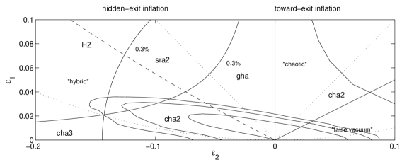
Figure 1: Observational constraints, interpretation, and accuracy of various approximations in the $\epsilon_{1}$–$\epsilon_{2}$ plane: the likelihood curves have been provided by S. M. Leach [24] and enclose the $1\sigma$-, $2\sigma$- and $3\sigma$-allowed regions. Models with a scale-invariant spectrum fall on the dashed line (HZ). An observation of $\epsilon_{2}>0$ would favour simple models of inflation, in which the evolution toward a graceful exit is seen (toward-exit inflation). If $\epsilon_{2}\leq 0$, a more contrived scenario must be realized, since in that case the mechanism of exit is hidden from observation (hidden-exit inflation). The region with $\epsilon_{2}>0$ is further split up by the (full straight) line $\epsilon_{1}=\epsilon_{2}/2$, which distinguishes models in which the kinetic energy density decreases (above the line) or increases with time. The latter requires a mechanism to ensure that the kinetic energy density is very small initially. The solid arc centered at the origin encloses the region in which the slow-roll approximation at second order (sra2) provides a prediction of the amplitude at the pivot scale better than $0.3\%$. Below the hyperbolic lines the same accuracy is achieved for the constant-horizon approximation (cha2 at second order, cha3 at third order) and the growing horizon approximation (gha). The dotted lines represent the boundaries between cha3 and cha2, as well as between cha2 and gha.

Based on the observational constraints on the first two horizon-flow functions, we do not restrict our considerations to slow-roll models in this paper. We relax the slow-roll conditions ($\epsilon_{m}\ll 1$ for all $m$) to $\epsilon_{m}\leq 1$ for some $m$. In Section 2 we demonstrate that the condition $\epsilon_{1}\ll 1$ is sufficient to guarantee that the Hubble scale is almost constant during the inflationary epoch of interest.

The physical meaning of the first and second horizon-flow functions is discussed in Section 3 in the framework of single-field models, and a new physical classification of inflationary scenarios is introduced, based on the behaviour of the kinetic and total energy densities of the inflaton. To our surprise this approach closely resembles the small field/large field/hybrid classification of Dodelson et al. [29], but is not restricted to slow-roll models.

In Section 4 we derive a procedure to self-consistently calculate higher-order corrections at any scale $k$, given an analytic expression of the power at the pivot scale $k_{*}$ as a function of the horizon-flow functions. A similar relation has been used in the literature to calculate the spectral index and its running so far, but, to our knowledge, it has never been justified rigorously.

Starting from the observation that $\epsilon_{1}\ll 1$, we show that the slow-roll approximation is no longer needed in the analysis of the data and that it could be replaced by a more efficient approximation (constant-horizon approximation [11]). The latter is more efficient in the sense that we need to know less horizon-flow functions in order to predict the power spectra to a given accuracy, as compared with the slow-roll approximation.

We map the classification of models from the $\epsilon_{1}$–$\epsilon_{2}$ plane to the space spanned by the tilt of the spectrum, $n-1$, and the ratio of tensor and scalar amplitudes $r$ in Section 5. At leading order in the horizon-flow functions this is a one-to-one mapping; including higher orders introduces an ambiguity, due to the running of the spectral index. We thus argue that the $\epsilon_{1}$–$\epsilon_{2}$ plane is more fundamental. For practical purposes, the $r$–tilt plane is nevertheless a useful tool.

In Section 6 we give examples to demonstrate the accuracy of the new method and discuss the applicability of the new method in the light of the recent data.

Our main results are summarized in Fig. 1. We overlay our new classification of models on the likelihood contours as obtained by Leach and Liddle [24]. We also indicate which approximation to the power spectrum at the pivot scale is best suited for which region of parameter space. We assume an accuracy goal of $0.3\%$ at the pivot, which puts the theoretical errors safely away from the systematic and statistical errors of WMAP and Planck.

2 Hubble horizon flow during inflation

The Hubble horizon, $d_{\rm H}\equiv c/H$ (recall that $c=1$), is roughly the size of the region where causal processes can take place during one Hubble time $1/H$. An inflationary epoch is characterized by a decreasing comoving Hubble horizon, $d_{\rm H}/a$. Constant vacuum energy is the simplest (but unphysical, since inflation would continue forever) kind of matter leading to an inflationary universe. In this scenario, the Hubble scale is constant. More generally, during inflation, $d_{H}$ is expected to vary slowly during a given number of e-foldings $N$: ${\rm d}N/{\rm d}t=H$. The behaviour of the Hubble horizon can be parameterized as

$$d_{\rm H}(N) = d_{\rm H}(N_{*})\left[1+\epsilon_{1}(N-N_{*})+\frac{1}{2}(\epsilon_{1}^{2}+\epsilon_{1}\epsilon_{2})(N-N_{*})^{2}+\cdots\right]\,,$$ (5)

where the coefficients in this expansion are expressed in terms of the horizon-flow functions $\epsilon_{m}$ at the pivot point. One can see that, if $\epsilon_{1}\ll 1$ and $\epsilon_{m}<1$ for any $m>1$, then $d_{\rm H}\approx$ constant. For such cases, the smaller $\epsilon_{1}$ is, the larger the other horizon-flow functions can be, since $\epsilon_{1}$ is the leading factor of all coefficients of the higher-order terms in the series. We can use this observation as the starting point for what we call the constant-horizon approximation ($\epsilon_{1}\ll 1$ and $\epsilon_{m}<1$ for all $m>1$). As is seen in Fig. 1 and discussed in the introduction, the data show that $\dot{d}_{\rm H}\equiv\epsilon_{1}\ll 1$.

3 Classification of single scalar field inflationary models

The number of proposed models of cosmological inflation is very large and keeps growing. Current observations allow us to constrain the number of successful models, and future observations are expected to play a stronger role in that direction. For a more effective use of the data analysis, it is useful to group the inflationary scenarios according to some commonly applicable criteria, i.e. independent of parameters such as masses or coupling constants, which are strongly model-dependent. For slow-roll inflation, such a classification was suggested by Dodelson, Kinney and Kolb [29], based on the shape of the inflaton potential (and expressed as conditions on the slow-roll parameters).

Here we present a new scheme in terms of the horizon-flow functions, which closely resembles the Dodelson et al. classification, but avoids misleading terminology, allows the inclusion of models beyond the slow-roll class, and is based on physical criteria on the kinetic and total energy densities.

The idea is to investigate how the kinetic and potential energy of the inflaton field change with time, both absolute and relative to each other. It is thus useful to rewrite the first two horizon-flow functions as

$$\epsilon_{1}=3{\dot{\varphi}^{2}/2\over\dot{\varphi}^{2}/2+V}\,,$$ (6)

$$\epsilon_{2}=2\left({\ddot{\varphi}\over H\dot{\varphi}}+\epsilon_{1}\right)\,,$$ (7)

where we used Eqs. (1) and (2). Using Eqs. (1) and (7), the time variation of the potential energy is found to be

$$\dot{V}=-H\dot{\varphi}^{2}\left(3-\epsilon_{1}+\frac{\epsilon_{2}}{2}\right).$$ (8)

Since $H\dot{\varphi}^{2}>0$, the potential energy density can never increase for physically meaningful values of $\epsilon_{1}$ and $\epsilon_{2}$. Thus, we focus on the behaviour of the kinetic energy density.

According to Eq. (6), $\epsilon_{1}/3\geq 0$ measures the ratio of kinetic energy density to total energy density. Using definition (3), we can ask how this ratio changes with time during inflation:

$$\frac{\rm d}{{\rm d}t}\frac{\epsilon_{1}}{3}=H\frac{\epsilon_{1}}{3}\epsilon_{2}.$$ (9)

Since $H$ and $\epsilon_{1}$ are positive, $\epsilon_{2}=0$ marks a borderline between two physically different cases: increasing ($\epsilon_{2}>0$) and decreasing ($\epsilon_{2}<0$) kinetic energy density with respect to the total energy density of the inflaton.

For a more complete understanding of the inflationary dynamics, we must also look at the absolute time variation of the kinetic energy density ${\rm d}{(\dot{\varphi}^{2}/2)}/{\rm d}t$, which, using Eqs. (1) and (8), can be written as

$$\dot{\varphi}\ddot{\varphi}=H\dot{\varphi}^{2}\left(\frac{\epsilon_{2}}{2}-\epsilon_{1}\right).$$ (10)

For $\epsilon_{1}>0$ we have $\dot{\varphi}\neq 0$ and thus $\epsilon_{2}=2\epsilon_{1}$ is another borderline between two different physical scenarios in which kinetic energy density grows ($\epsilon_{2}>2\epsilon_{1}$) or falls ($\epsilon_{2}<2\epsilon_{1}$) with time. We thus arrive at the following classification:

• $\epsilon_{2}>0$: the kinetic energy density is increasing with respect to the total energy density. This is a necessary condition for evolving toward a graceful exit of inflation. Thus, such models could be called toward-exit models, since it can be argued that the approach to a graceful exit of inflation is observed in that case (although a more complicated interpretation remains possible).

  There are two subcases, corresponding to whether or not the kinetic energy density grows with time. It would be expected that this provides a criterion to discriminate between the false vacuum models and chaotic models in the slow-roll phase, since false vacuum models start out with vanishing kinetic energy density, whereas chaotic models always have a non-vanishing kinetic energy density.

  • $\epsilon_{2}>2\epsilon_{1}$: kinetic energy density grows with time. An example of this are false vacuum models arising, e.g. in superstrings models, with potential $V=V_{0}-m^{2}\varphi^{2}/2$ [30]. Here, in the slow-roll phase, $\epsilon_{2}\approx 4(V_{0}/m^{2}\varphi^{2})\epsilon_{1}$, and the condition is met as long as $V_{0}>m^{2}\varphi^{2}/2$. False vacuum models need to provide a mechanism that gives rise to small kinetic energy density of the inflaton before observable modes cross the Hubble scale during inflation.

  • $\epsilon_{2}<2\epsilon_{1}$: kinetic energy density is decreasing with time. Monomial potentials $V=\lambda\varphi^{n}/n$ with chaotic initial conditions give rise to models of that kind. During their slow-roll phase $\epsilon_{2}\approx(4/n)\epsilon_{1}$, and the criterion is met for $n>2$. Here no extra mechanism is needed to tune the kinetic energy density initially, and one could argue that these are the simplest models.

  • $\epsilon_{2}=2\epsilon_{1}$: kinetic energy density is constant. For slow-roll models, this is realised for chaotic inflation with a quadratic potential ($n=2$) [31].

    Note that this criterion is different from the one given by Dodelson et al. [29] to distinguish between small- and large-field models. In our notation and in the slow-roll approximation their borderline is $\epsilon_{2}\simeq 4\epsilon_{1}$. This is the case of a linear potential ($n=1$). Naively one would think that these models should fall into the same class as chaotic inflationary models, but actually they do not give rise to a successful scenario, since for the linear potential $V=V_{0}(1+\varphi/\varphi_{0})$ we find during slow-roll $\epsilon_{1}\approx\epsilon_{2}/4\approx 1/(2\varphi_{0}^{2})$, which is constant and thus inflation never ends.

• $\epsilon_{2}<0$: kinetic energy density is decreasing absolutely and relatively. Here, in order to reach a graceful exit, $\epsilon_{2}$ has to change sign at some point. Thus, negative values of $\epsilon_{2}$ must correspond to models in which inflation still has to go through a transition to either another stage of inflation or to directly to stop it by some unknown mechanism. The actual mechanism of exit is out of sight of observations, so we could call these models hidden-exit models.

  An example is the hybrid model, with an effective potential $V=V_{0}+m^{2}\varphi^{2}/2$ in the slow-roll phase [32]. In that case $\epsilon_{2}\approx-4(V_{0}/m^{2}\varphi^{2})\epsilon_{1}$. In order to end inflation $V_{0}$ must depend on yet another field which finally drives $V_{0}$ to zero.

• $\epsilon_{2}=0$: the ratio of kinetic to total energy density is constant. If additionally all $\epsilon_{m}=0$, then this is de Sitter space-time. If only $\epsilon_{1}\neq 0$, then this is power-law inflation [33]. There also exists a number of models where $\epsilon_{2}$ asymptotically converges to zero during inflation, so that they are observationally indistinguishable from power-law inflation (see [34] for a discussion and further references). In all these cases there is no exit from inflation but the models are not ruled out by current cosmological data.

  Provided the slow-roll approximation holds, $\epsilon_{2}=0$ coincides with the limit between hybrid models and large-field models in the Dodelson et al. classification.

Summarizing, our three classes are i) hidden-exit inflation ($\epsilon_{2}\leq 0$), ii) toward-exit inflation with general (“chaotic”) initial conditions ($0<\epsilon_{2}\leq 2\epsilon_{1}$), and iii) toward-exit inflation with special (e.g. false vacuum) initial conditions ($0<2\epsilon_{1}<\epsilon_{2}$).

At this point it is convenient to note that the here introduced by us classification involves only exact expressions. We confront this new classification with the observational constraints in Fig. 1. Although the biggest piece of allowed parameter space falls into the hidden-exit inflation class, this cannot be seen as a preference of the data for this scenario, since the shape of the likelihood curves is due to the tensor degeneracy. At present all scenarios are consistent with the data. A better determination of the spectral index (lines parallel to the dashed line correspond roughly to fixed values of the spectral index) could in principle rule out some of the possibilities; there is thus hope to learn more about inflation, well before we can expect to get a hand on the tensor contribution via observations of the B-polarization pattern of the CMB.

4 Power spectra

The accurate prediction of inflationary perturbations have been of concern since Mukhanov and Chibisov [4] realized that density and space-time perturbations during inflation could be the seeds for large-scale structure formation. The calculation of inflationary power spectra requires the solution of the mode equations for scalar and tensor fluctuations. The assumption that scalar and tensor perturbations are quantum fluctuations of the vacuum originally fixes the power spectra uniquely. The mode equations are of the same type as the Schroedinger equation, which happens to be difficult to solve, even for the simple models (see [35, 36, 37, 38, 11, 12, 39] for details and references).

It proved useful to expand the primordial power spectrum in a Taylor series around a pivot scale $k_{*}=(aH)(N_{*})$. Within a time interval $\Delta t\sim 1/H$, the modes in the logarithmic frequency interval $\Delta\ln k=\ln(eaH)-\ln(aH)=1$ cross the Hubble scale. It is thus natural to expand in terms of $\ln(k/k_{*})$:

$${\cal P}(k)=\tilde{\cal P}(k_{*})\sum_{n\geq 0}{a_{n}\over n!}\ln^{n}\left(\textstyle{k\over k_{*}}\right),$$ (11)

where the coefficients are defined by

$$a_{n}(k_{*})={{\rm d}^{n}\over{\rm d}\ln^{n}k}\left.{{\cal P}(k)\over\tilde{\cal P}(k_{*})}\right|_{k=k_{*}}.$$ (12)

These coefficients depend on the horizon-flow parameters in such a way that they are regular in the limit $\epsilon_{m}\to 0$; in fact $a_{0}\to 1$ and $a_{n}\to 0$ for all $n>0$. Now it becomes obvious why we have separated a factor that represents the leading-order prediction for the amplitude at the pivot scale

$$\tilde{\cal P}_{\rm S}(k_{*})\equiv{H_{*}^{2}\over 8\pi^{2}\epsilon_{1}}$$ (13)

for scalar perturbations, and

$$\tilde{\cal P}_{\rm T}(k_{*})\equiv{2H_{*}^{2}\over\pi^{2}}$$ (14)

for tensor perturbations. In the notation of the WMAP team, ${\cal P}_{\rm S}(k_{*})\equiv 10^{-9}A$ and ${\cal P}_{\rm T}(k_{*})/{\cal P}_{\rm S}(k_{*})\equiv r$.

4.1 Independence from the pivot point

The physical power spectrum must not depend on the arbitrary choice of a pivot scale $k_{*}$ in the above expansion:

$${{\rm d}{\cal P}(k)\over{\rm d}\ln k_{*}}\equiv 0\,.$$ (15)

Evaluation of this expression provides us with the non-trivial relation

$$\sum_{n\geq 0}{1\over n!}\ln^{n}\left({k\over k_{*}}\right)\left[{{\rm d}\ln\tilde{\cal P}\over{\rm d}\ln k_{*}}a_{n}+{{\rm d}a_{n}\over{\rm d}\ln k_{*}}\right]-\sum_{n\geq 1}{a_{n}\over(n-1)!}\ln^{n-1}\left({k\over k_{*}}\right)=0\,.$$ (16)

A comparison of the coefficients of $\ln^{n}(k/k_{*})$ finally leads to a recursion relation for the higher coefficients of the Taylor series:

$$a_{n+1}={1\over 1-\epsilon_{1}}\left[{{\rm d}a_{n}\over{\rm d}N_{*}}+{{\rm d}\ln\tilde{\cal P}\over{\rm d}\ln N_{*}}a_{n}\right]\quad\forall n\geq 0\,,$$ (17)

where in the last step we used the identity

$${\rm d}\ln k_{*}=(1-\epsilon_{1}){\rm d}N_{*}\,.$$ (18)

For scalars ${\rm d}\ln\tilde{\cal P}_{\rm S}/{\rm d}\ln N_{*}=-2\epsilon_{1}-\epsilon_{2}$, whereas for tensors ${\rm d}\ln\tilde{\cal P}_{\rm T}/{\rm d}\ln N_{*}=-2\epsilon_{1}$. Let us note that the recursion relation (17) is an exact result: no approximation has been made, apart from the assumption that the linear perturbation analysis is justified.

4.2 Approximation schemes

Up to date, three approximation schemes have been proposed to allow for a high-precision calculation of the spectra amplitudes. Using recursion (17), all of these approximations yield expressions for the coefficients $a_{n}$ as expansions in terms of the horizon-flow functions. Keeping terms up to order $\epsilon^{q}$ (which stands here for any monomial of $\epsilon_{m}$’s at order $q$) in $a_{0}$ allows us to calculate all terms up to order $\epsilon^{q+n}$ in $a_{n}$. We will denote the order of a given approximation by the highest order in the seed $a_{0}$. Besides the order $q$, a second choice that must be made prior to data analysis is how many coefficients $a_{n}$ should be included in the analysis. The common practice is that only the terms $a_{0}$ and $a_{1}$ are taken into account, $a_{2}$ being included when the running of the spectral index is included.

4.2.1 Slow-roll approximation.

Assuming all horizon-flow functions to be small (without assuming any hierarchy among them), the equation of modes can be solved by an iterative method using Green’s functions [38]. To second order in the slow-roll parameters, here expressed as horizon-flow parameters, the seed for recursion (17) for the scalar spectrum reads

$$a_{{\rm S}0} = 1-2(C+1)\epsilon_{1}-C\epsilon_{2}$$ (19)

$$+\left(2C^{2}+2C+\frac{\pi^{2}}{2}-5\right)\epsilon_{1}^{2}+\left(\frac{C^{2}}{2}+\frac{\pi^{2}}{8}-1\right)\epsilon_{2}^{2}$$

$$+\left(C^{2}-C+\frac{7\pi^{2}}{12}-7\right)\epsilon_{1}\epsilon_{2}+\left(-\frac{C^{2}}{2}+\frac{\pi^{2}}{24}\right)\epsilon_{2}\epsilon_{3}\,,$$

where $C\equiv\gamma_{\rm E}+\ln 2-2\approx-0.7296$, while for the tensor spectrum we have [12],

$$a_{{\rm T}0} = 1-2(C+1)\epsilon_{1}$$ (20)

$$+\left(2C^{2}+2C+\frac{\pi^{2}}{2}-5\right)\epsilon_{1}^{2}+\left(-C^{2}-2C+\frac{\pi^{2}}{12}-2\right)\epsilon_{1}\epsilon_{2}\,.$$

In Fig. 1 we estimated the region of parameter space in which the prediction of the pivot amplitude $A(k_{*})$ is better than $0.3\%$ for the slow-roll approximation at second order. Such a high precision is actually needed to ensure that the power spectrum can be predicted with an accuracy better than a few per cent over at least three or four decades in wave number.

4.2.2 Constant-horizon assumption.

In a number of inflationary models the time derivative of the Hubble distance is tiny (see Section 6 for examples). For this kind of models, during a certain number of e-foldings, $\epsilon_{1}\ll 1$. However, as we have seen in Section 2, this does not necessarily mean that all other $\epsilon_{m}$ have to be small as well. We thus worked out the constant-horizon approximation [11] at order $q$ for the situation $|\epsilon_{2}^{q}|>\max(|\epsilon_{1}\epsilon_{2}|,|\epsilon_{2}\epsilon_{3}|)$, which means that, for $a_{0}$ we are allowed to include the following monomials in the primordial spectra: $1,\epsilon_{1},\epsilon_{2},\dots,\epsilon_{2}^{q}$. With this approximation, the $q=3$ expression for the seed of the scalar spectrum is

$$a_{{\rm S}0} = 1-2(C+1)\epsilon_{1}-C\epsilon_{2}+\left(\frac{C^{2}}{2}+\frac{\pi^{2}}{8}-1\right)\epsilon_{2}^{2}$$ (21)

$$-\left(\frac{C^{3}}{6}-C+C\frac{\pi^{2}}{8}+\frac{7}{8}\zeta(3)-\frac{2}{3}\right)\epsilon_{2}^{3}\,,$$

where $\zeta(3)\approx 1.2021$, and to any order for the tensor spectrum,

$$a_{{\rm T}0} = 1-2(C+1)\epsilon_{1}\,.$$ (22)

Also here we estimate the region of $0.3\%$ accuracy of $A(k_{*})$ and indicate it in Fig. 1. For more details on how to do this we refer the reader to the work of [11].

4.2.3 Growing-horizon assumption.

This approximation is valid for cases with $|\epsilon_{m}|<\epsilon_{1}$ for $m>1$. The trivial example here is power-law inflation [33], where only $\epsilon_{1}\neq 0$. This approximation is also valid in inflationary scenarios, where power-law inflation dynamics is a past or future attractor, and $\epsilon_{1}$ is sufficiently large for higher-order corrections to make sense. An expression for $a_{0}$ can be obtained by keeping all terms in $\epsilon_{1}$ up to order $q$, where $q$ is the maximal integer for which $\epsilon_{1}^{q}>\max(|\epsilon_{1}\epsilon_{2}|,|\epsilon_{2}\epsilon_{3}|)$ holds true. We defined the (linearly) growing-horizon approximation to order $q$ [11] to include the following terms: $1,\epsilon_{1},\dots,\epsilon_{1}^{q},\epsilon_{2}$. To third order the corresponding expression for the scalar spectrum is

$$a_{{\rm S}0} = 1-2(C+1)\epsilon_{1}+\left(2C^{2}+2C+\frac{\pi^{2}}{2}-5\right)\epsilon_{1}^{2}$$ (23)

$$-\ \left(\frac{4C^{3}}{3}+C\pi^{2}-12C+\frac{14}{3}\zeta(3)-\frac{19}{3}\right)\epsilon_{1}^{3}-C\epsilon_{2}\,,$$

and for the tensor spectrum,

$$a_{{\rm T}0} = 1-2(C+1)\epsilon_{1}$$ (24)

$$+\left(2C^{2}+2C+\frac{\pi^{2}}{2}-5\right)\epsilon_{1}^{2}$$

$$-\ \left(\frac{4C^{3}}{3}+C\pi^{2}-12C+\frac{14}{3}\zeta(3)-\frac{19}{3}\right)\epsilon_{1}^{3}\,.$$

5 Classification of inflation models in the $r$–tilt plane

In this section we indicate how to make contact with the variables that are frequently used in cosmological parameter estimation. However useful these variables have been assumed to be so far, as we shall see here, the analysis using them becomes much more involved that while using the horizon-flow functions. Complications arise because there are not exact model independent expressions for $(n-1)$ and $r$; they are given as expansions in terms of the horizon-flow functions.

Using one or the other set of variables is just a matter of choosing the working parametrization for the primordial spectra. Very often a power-law shape is assumed for the scalar power spectrum;

$${\cal P}_{\rm S}(k)=A(k_{*})\left(k\over k_{*}\right)^{n-1},$$ (25)

where $n$ is called the spectral index and $n-1$ the tilt of the spectrum. A comparison with expression (11) reveals that

$$A(k_{*}) = \tilde{{\cal P}}(k_{*})a_{{\rm S}0},$$ (26)

$$(n-1)(k_{*}) = {a_{{\rm S}1}\over a_{{\rm S}0}}.$$ (27)

For the slow-roll and the constant-horizon approximation we find at second order in the horizon-flow functions

$$(n-1)(k_{*})=-2\epsilon_{1}-\epsilon_{2}-2\epsilon_{1}^{2}-(2C+3)\epsilon_{1}\epsilon_{2}-C\epsilon_{2}\epsilon_{3}.$$ (28)

A difference between the two approximations shows up at the third order. Here we restrict the discussion to the second order expressions.

Tensor contributions are typically introduced via the tensor to scalar ratio

$$r={{\cal P}_{\rm T}(k_{*})\over{\cal P}_{\rm S}(k_{*})}=16\epsilon_{1}(1+C\epsilon_{2})$$ (29)

at second order in the slow-roll and the constant-horizon approximation.

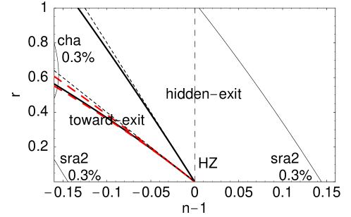
Figure 2: Classification of models in the $r$–tilt plane. The vertical long dashed line denotes the scale-invariant HZ spectrum. Toward-exit models of inflation have a negative tilt (red spectrum) and are found to the l.h.s. of the upper full line. To the r.h.s. of the upper full line we find the hidden-exit models. The (upper) short dashed line shows the approximate borderline derived from the leading order expression given in the text. The toward-exit models are divided by another thick line which assumes vanishing running of the spectral index. Models with decreasing kinetic energy are confined between both thick lines. The (lower) short dashed line is the approximate leading order result. The tilted long dashed lines show two cases of non-vanishing running of the spectral index, namely ${\rm d}n/{\rm d}\ln k=-12\epsilon_{1}^{2}(+4\epsilon_{1}^{2})$, corresponding to $\epsilon_{3}=+2\epsilon_{2}(-2\epsilon_{2})$. The upper curve corresponds to the negative sign of the running. We also indicate the accuracy of the considered approximations.

A closer inspection of the above expressions shows that there is a simple one-to-one map $(\epsilon_{1},\epsilon_{2})\leftrightarrow(r,n-1)$ at the leading order, namely $\epsilon_{1}=r/16$ and $\epsilon_{2}=-r/8-(n-1)$. Thus the physical classification of single scalar field models is characterized by the borderlines $\epsilon_{2}=0\Leftrightarrow r=-8(n-1)$ and $\epsilon_{2}=\epsilon_{1}/2\Leftrightarrow r=-4(n-1)$ (short dashed lines in Fig. 2).

This one-to-one correspondence is spoiled by the $\epsilon_{3}$-dependence of $n-1$ at the second order. Nevertheless, the borderline $\epsilon_{2}=0$ (upper full line in Fig. 2) is well defined, since higher horizon-flow parameters enter only together with $\epsilon_{2}$ and thus it is in principle possible to distinguish toward-exit inflation from hidden-exit inflation in the $r$-tilt plane.

However, the borderline ($\epsilon_{2}=\epsilon_{1}/2$) between the two subclasses of toward-exit models, i.e., models with general initial conditions and models with special initial conditions, gives rise to a family of lines that depends on the observed running of the spectral index, ${\rm d}n/{\rm d}\ln k=-2\epsilon_{1}\epsilon_{2}-\epsilon_{2}\epsilon_{3}$ (leading order). One possibility is to fix $\epsilon_{3}$ by assuming that the leading contribution to the running vanishes (lower full line in Fig. 2). Thus it is impossible to distinguish between models with decreasing (“chaotic”) and increasing (“false vacuum”) kinetic energy density on the basis of a $r$–tilt plot, unless the running of the spectral index is known or constrained to be small.

The above discussion confirms that the horizon-flow functions are more fundamental than other quantities that have been used to classify inflation models. However, the upper solid line in Fig. 2 is robust in the sense that it holds true for the slow-roll approximation and the constant-horizon approximation at any order (as terms $\epsilon_{n}$ with $n>2$ enter in combination with $\epsilon_{2}$ and are thus zero for $\epsilon_{2}=0$).

Figure 2 shows another remarkable feature of the constant and growing horizon approximations: for the shown region in $r$ and $n-1$ the amplitudes are accurate to $0.3\%$, except for the tiny region enclosed by the arc on the l.h.s. of the figure. This is in contrast to the slow-roll approximation at second order, which is less accurate in the upper right and lower left corner of the figure.

6 Testing the higher-order constant-horizon approximation

As we already noted, observations show that $\epsilon_{1}\ll 1$. If $\epsilon_{2}$ is of the order of $\epsilon_{1}$ or smaller, higher-order corrections (terms that are at least quadratic in the horizon-flow functions) to the primordial spectra are irrelevant and the first-order expression for $a_{0}$, the seed of the recursion (17), is good enough to calculate the coefficients $a_{n}$ in the power spectrum (11). Nevertheless, if $\epsilon_{2}$ is actually much larger than $\epsilon_{1}$, then higher-order corrections in $\epsilon_{2}$ could be necessary to match the observational accuracy. In such a case the constant-horizon approximation (see Section 4.2.2) is the simplest and most economic way of obtaining high-precision predictions. To see if this is true, let us start by comparing Eqs. (19) and (21). One sees that the third-order expression for the constant-horizon approximation is simpler and requires knowledge of less horizon-flow functions than the corresponding lower-order slow-roll approximation. Next, we must test how good the constant-horizon approximation is.

To measure the error of the approximations, we define

$$\Delta A(\log\tilde{k})=\frac{A_{\rm num}(\log\tilde{k})-A_{\rm appr}(\log\tilde{k})}{A_{\rm num}(\log\tilde{k})}\,100\%\,,$$ (30)

where $A_{\rm num}(\log\tilde{k})$ and $A_{\rm appr}(\log\tilde{k})$ stand for the numerical and analytically approximated values of the amplitudes at the normalized scale $\tilde{k}\equiv k/k_{*}$.

The constant-horizon approximation applies for many single-field models based on phenomenological particle physics: the inverted quadratic model $V=V_{0}-m^{2}\varphi^{2}/2$ [30], or more generally models with $V=V_{0}[1-(\varphi/\mu)^{p}]$ and $p\geq 2$, and also for those with $V=V_{0}(1-\exp(-\varphi/\mu))$ [41]. For positive $\mu$, all these models belong to the class of toward-exit inflation with special initial conditions. There are also examples of hybrid inflation models, e.g. those arising from dynamical supersymmetry breaking with $V=V_{0}[1\pm(\mu/\varphi)^{p}]$, where $p$ is a positive integer [42]. For the positive sign, the model belongs to the hidden-exit inflation class, while for the negative sign, the models belong to the class of toward-exit inflation with special initial conditions. Yet another model belonging to that class is hybrid inflation with a running mass that arises from one-loop corrections in supersymmetry-inspired models (see Refs. [43, 44, 45] for concrete realizations):

$$V=V_{0}\left[1-\frac{1}{2}m^{2}(\varphi)\varphi^{2}\right]\,.$$ (31)

Further examples where the constant-horizon approximation applies are the so-called natural inflation model [40]:

$$V=\Lambda^{4}\left[1+\cos\left(N\frac{\varphi}{f}\right)\right]\,,$$ (32)

and the model proposed by Wang et al. [36],

$$V=\Lambda^{4}\left[1-\frac{2}{\pi}\arctan\left(5\varphi\right)\right]\,,$$ (33)

which is a designer model that has been used to demonstrate the limitations of the slow-roll approximation.

We started by testing the natural inflation model given by potential (32). For this model with $\Lambda=f=1$ and $N=1$ at the pivot value $\varphi_{*}=0.01$, we obtained $H_{*}=0.81648$, $\epsilon_{1}\approx\epsilon_{3}\approx 10^{-7}$, $\epsilon_{2}\approx 0.039529$ and $\epsilon_{4}\approx 0.02008$. With these values, we find that the third-order constant-horizon approximation performs slightly better than the second-order slow-roll approximation, and that both of them provide a significant improvement with respect to the first order slow-roll approximation. The errors are confined within the $15\%$ interval in a range exceeding $\Delta\log\tilde{k}=6$.

More interesting is a test for a model where some of the higher horizon-flow functions are “large”. We start from Eq. (31) and use the ad hoc choice $m^{2}(\varphi)=M^{2}\exp\left(-\varphi/\mu\right)$, with $M$ and $\mu$ positive. The resulting potential has a maximum at $\varphi=0$ and a minimum at $\varphi=2\mu$. Starting near the false vacuum, enough inflation can be produced before the minimum is reached. For $V_{0}=1$, $\mu=1$ and $M=2$ at the pivot value $\varphi_{*}=0.01$, we find $H_{*}=0.57729$, $\epsilon_{1}=0.00003$, $\epsilon_{2}=0.29494$, $\epsilon_{3}=-0.00381$, $\epsilon_{4}=0.14344$ and $\epsilon_{5}=-0.0082$, with the results presented in Figs. 3, 4 and 5.

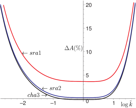
Figure 3: Test of approximated solutions to the equation of the scalar modes for a hybrid model with running mass. Third-order constant-horizon approximation (cha3), and first (sra1) and second (sra2) order slow-roll approximations are compared. The errors shown are those obtained including terms up to $a_{3}$ in parametrization (11) and keeping the highest possible order for the horizon-flow functions in all coefficients.

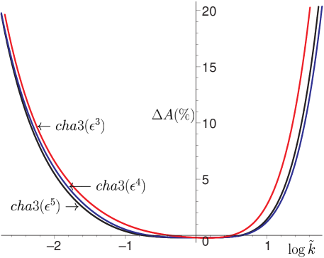
Figure 4: Test of the constant-horizon approximation for a hybrid model with running mass. The errors shown are those obtained including terms up to $a_{3}$ in parametrization (11), and varying the order of the highest included horizon-flow function.

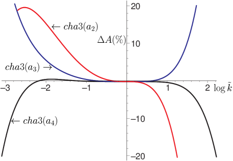
Figure 5: Test of the constant-horizon approximation for a hybrid model with running mass. Here we investigate the convergence of the Taylor expansion (11) as more and more coefficients $a_{n}$ are added. We keep the highest possible order of the horizon-flow functions.

As can be observed in Fig. 3, the conclusions drawn for the simple inflation near a maximum model are still valid for models where the conditions for constant-horizon approximation to apply are met in a weaker fashion than in the case of natural inflation, although the range where the errors are confined in the $15\%$ error band is smaller. According with the results in Fig. 4, increasing the order of the horizon-flow functions beyond the quadratic in every included term of parametrization (11) does not significantly improve the accuracy of the approximation.

As shown in Fig. 5, adding terms in parametrization (11) actually seems to be most important for increasing the precision of the prediction, but this conclusion might not hold true for other models. Even in the best case, it seems difficult to keep the error below the $15\%$ mark for a range broader that $\Delta\log\tilde{k}=5$.

We tried to push our approximation to the limits by testing it on the model given by Eq. (33). For $\Lambda=1$ and $\varphi_{*}=-0.25$, we find $H_{*}=0.72476$, $\epsilon_{1}=0.01122$, $\epsilon_{2}=0.31874$, $\epsilon_{3}=0.19659$, $\epsilon_{4}=0.079$ and $\epsilon_{5}=0.129$. The test confirms the previous results, although the range where the error is under $15\%$ is significantly shorter, $\Delta\log\tilde{k}\approx 3.5$.

For completeness we note here that similar results were obtained for the tensor modes.

For all tested cases, the constant-horizon approximation at third order performed as good or slightly better than the slow-roll approximation at second order, but it has the advantage that one needs to make less restrictive assumptions on higher horizon-flow functions and the approximation is more efficient in the sense that the recursion seed $a_{0}$ only needs $\epsilon_{1}$ and $\epsilon_{2}$ as an input, whereas the slow-roll approximation at second order needs additionally $\epsilon_{3}$.

References

References

- [1] Bennett C L et al., First year Wilkinson Microwave Anisotropy Probe (WMAP) observations: preliminary maps and basic results, 2003 Astrophys. J. Suppl. 148 1 [astro-ph/0302207]
- [2] Spergel D N et al., First year Wilkinson Microwave Anisotropy Probe (WMAP) observations: determination of cosmological parameters, 2003 Astrophys. J. Suppl. 148 175 [astro-ph/0302209]
- [3] Tegmark M et al. [SDSS Collaboration], The 3D power spectrum of galaxies from the SDSS, 2003 [astro-ph/0310725]
- [4] Mukhanov V F and Chibisov G V, Quantum fluctuation and ‘nonsingular’ universe, 1981 JETP Lett. 33 532 [Pisma Zh. Eksp. Teor. Fiz. 33 549]
- [5] Starobinsky A A, Spectrum of relict gravitational radiation and the early state of the universe, 1979 JETP Lett. 30 682 [Pisma Zh. Eksp. Teor. Fiz. 30 719]
- [6] Benoit A et al. [Archeops Collaboration], Cosmological constraints from Archeops, 2003 Astron. Astrophys. 399 L25 [arXiv:astro-ph/0210306]
- [7] Kovac J et al., Detection of polarization in the cosmic microwave background using DASI, 2002 Nature 420 772 [arXiv:astro-ph/0209478]
- [8] Kogut A et al., Wilkinson Microwave Anisotropy Probe (WMAP) First Year Observations: TE polarization, 2003 Astrophys. J. Suppl. 148 161 [arXiv:astro-ph/0302213]
- [9] Komatsu E et al., First Year Wilkinson Microwave Anisotropy Probe (WMAP) Observations: Tests of Gaussianity, 2003 Astrophys. J. Suppl. 148 119 [arXiv:astro-ph/0302223]
- [10] Liddle A R, Parsons P and Barrow J D, Formalizing the slow-roll approximation in inflation, 1994 Phys. Rev. D 50 7222 [astro-ph/9408015].
- [11] Schwarz D J, Terrero-Escalante C A and Garcia A A, Higher order corrections to primordial spectra from cosmological inflation, 2001 Phys. Lett. B 517 243 [astro-ph/0106020]
- [12] Leach S M, Liddle A R, Martin J and Schwarz D J, Cosmological parameter estimation and the inflationary cosmology, 2002 Phys. Rev. D 66 023515 [astro-ph/0202094]
- [13] Pearson T J et al., The Anisotropy of the Microwave Background to l = 3500: Mosaic Observations with the Cosmic Background Imager, 2003 Astrophys. J. 591 556 [astro-ph/0205388]
- [14] Benoit A et al. [Archeops Collaboration], The Cosmic Microwave Background Anisotropy Power Spectrum measured by Archeops, 2003 Astron. Astrophys. 399 L19 [astro-ph/0210305]
- [15] Kuo C L et al. [ACBAR collaboration], High Resolution Observations of the CMB Power Spectrum with ACBAR, 2002 [astro-ph/0212289]
- [16] Readhead A C S et al., Extended Mosaic Observations with the Cosmic Background Imager, 2004 [astro-ph/0402359]
- [17] Grainge K et al., The CMB power spectrum out to measured by the VSA, 2003 Mon. Not. Roy. Astron. Soc. 341 L23 [astro-ph/0212495]
- [18] Dickinson C et al., High sensitivity measurements of the CMB power spectrum with the extended Very Small Array, 2004 [arXiv:astro-ph/0402498]
- [19] Percival W J et al., The 2dF Galaxy Redshift Survey: the power spectrum and the matter content of the universe, 2001 Mon. Not. Roy. Astron. Soc. 327 1297 [astro-ph/0105252]
- [20] Tegmark M, Hamilton A J S and Xu Y, The power spectrum of galaxies in the 2dF 100k redshift survey, 2002 Mon. Not. Roy. Astron. Soc. 335 887 [astro-ph/0111575].
- [21] Peiris H V et al., First year Wilkinson Microwave Anisotropy Probe (WMAP) observations: Implications for inflation, 2003 Astrophys. J. Suppl. 148 213 [astro-ph/0302225]
- [22] Barger V, Lee H S and Marfatia D, WMAP and inflation, 2003 Phys. Lett. B 565 33 [hep-ph/0302150]
- [23] Kinney W H, Kolb E W, Melchiorri A and Riotto A, WMAPping inflationary physics, 2003 [hep-ph/0305130]
- [24] Leach S M and Liddle A R, Constraining slow-roll inflation with WMAP and 2dF, 2003 Phys. Rev. D 68 123508 [astro-ph/0306305]
- [25] Tegmark M et al. [SDSS Collaboration], Cosmological parameters from SDSS and WMAP, 2003 [astro-ph/0310723]
- [26] Rebolo R et al., Cosmological parameter estimation using Very Small Array data out to , 2004 [arXiv:astro-ph/0402466]
- [27] Efstathiou G, Principal Component Analysis of the Cosmic Microwave Background Anisotropies: Revealing The Tensor Degeneracy, 2001 Mon. Not. Roy. Astron. Soc. 332 193 [arXiv:astro-ph/0109151]
- [28] Schwarz D J, The first second of the universe, 2003 Annalen Phys. 12 220 [arXiv:astro-ph/0303574]
- [29] Dodelson S, Kinney W H and Kolb E W, Cosmic microwave background measurements can discriminate among inflation models, 1997 Phys. Rev. D 56 3207 [astro-ph/9702166]
- [30] Binétruy P and Gaillard M K, 1986 Candidates for the Inflaton Field in Superstring Models, Phys. Rev. D 34 3069
- [31] Linde A D, 1986 Eternally Existing Selfreproducing Chaotic Inflationary Universe, Phys. Lett. B 175 395
- [32] Linde A D, 1991 Axions in inflationary cosmology, Phys. Lett. B 259 38
- [33] Lucchin F and Matarrese S, Power Law Inflation, 1985 Phys. Rev. D 32 1316
- [34] Terrero-Escalante C A, 2003 Is power law inflation really attractive?, Rev. Mex. Fis. 49S2 118 [arXiv:astro-ph/0204066]
- [35] Stewart E D and Lyth D H, A more accurate analytic calculation of the spectrum of cosmological perturbations produced during inflation, 1993 Phys. Lett. B 302 171 [gr-qc/9302019]
- [36] Wang L M, Mukhanov V F and Steinhardt P J, On the problem of predicting inflationary perturbations, 1997 Phys. Lett. B 414 18 [astro-ph/9709032]
- [37] Martin J and Schwarz D J, The precision of slow-roll predictions for the CMBR anisotropies, 2000 Phys. Rev. D 62 103520 [arXiv:astro-ph/9911225]
- [38] Stewart E D and Gong J O, The density perturbation power spectrum to second-order corrections in the slow-roll expansion, 2001 Phys. Lett. B 510 1 [astro-ph/0101225]
- [39] Tsamis N C and Woodard R P, Improved estimates of cosmological perturbations, 2003 [arXiv:astro-ph/0307463]
- [40] Freese K, Frieman J A and Olinto A V, Natural Inflation With Pseudo - Nambu-Goldstone Bosons, 1990 Phys. Rev. Lett. 65 3233
- [41] Stewart E D, Inflation, supergravity and superstrings, Phys. Rev. D 51 (1995) 6847 [arXiv:hep-ph/9405389].
- [42] Kinney W H and Riotto A, A signature of inflation from dynamical supersymmetry breaking, Phys. Lett. B 435 (1998) 272 [arXiv:hep-ph/9802443].
- [43] Stewart E D, Flattening the inflaton’s potential with quantum corrections, 1997 Phys. Lett. B 391 34 [hep-ph/9606241].
- [44] Stewart E D, Flattening the inflaton’s potential with quantum corrections. 2, 1997 Phys. Rev. D 56 2019 [hep-ph/9703232].
- [45] Covi L, Hybrid inflation with running inflaton mass, 1999 Phys. Rev. D 60 023513 [hep-ph/9812232].