Towards the Theory of Binary Bound States in Quark-Gluon Plasma

Abstract

Although at temperatures $T\gg\Lambda_{QCD}$ the quark-gluon plasma (QGP) is a gas of weakly interacting quasiparticles (modulo long-range magnetism), it is strongly interacting in the regime $T=(1-3)\,T_{c}$. As both heavy ion experiments and lattice simulations are now showing, in this region the QGP displays rather strong interactions between the constituents. In this paper we investigate the relationship between four (previously disconnected) lattice results: i. spectral densities from MEM analysis of correlators; ii. static quark free energies $F(R)$; iii. quasiparticle masses; iv. bulk thermodynamics $p(T)$. We show a high degree of consistency among them not known before. The potentials $V(R)$ derived from $F(R)$ lead to large number of binary bound states, mostly colored, in $gq,qq,gg$, on top of the usual $\bar{q}q$ mesons. Using the Klein-Gordon equation and (ii-iii) we evaluate their binding energies and locate the zero binding endpoints on the phase diagram, which happen to agree with (i). We then estimate the contribution of all states to the bulk thermodynamics in agreement with (iv). We also address a number of theoreticall issues related with to the role of the quark/gluon spin in binding at large $\alpha_{s}$, although we do not yet include those in our estimates. Also the issue of the transport properties (viscosity, color conductivity) in this novel description of the QGP will be addressed elsewhere.

]

I Introduction

A New view of the Quark-gluon Plasma at not-too-high T

From its inception two decades ago, the high-T phase of QCD commonly known as the Quark-Gluon Plasma (QGP) after [1], was described as a weakly interacting gas of “quasiparticles” (quarks and gluons). Indeed, at very high temperatures asymptotic freedom causes the electric coupling to be small and the QGP to be weakly interacting or perturbative . At intermediate temperatures of few times the critical temperature $T_{c}$ of immediate relevance to current experiments, there is new and growing evidence that the QGP is not weakly coupled. In a recent letter [3] (to be referred to below as SZ1) we have proposed that in this region QCD seems to be close to a strongly coupled Coulomb regime, with an effective coupling constant $\alpha\approx 0.5-1$ and multiple bound states of quasiparticles. We have argued there (and will show it more quantitative below) that these bound states are very important for the thermodynamics of the QGP, responsible for roughly half of the pressure in RHIC domain. We will not address transport properties of the QGP in this paper, although we expect the bound states to play an even more important role.

To set the stage we first recall the chief arguments behind a scenario of strongly coupled QGP at such temperatures: i. a low viscosity argument; ii. recent lattice findings of $\bar{c}c,\bar{q}q$ bound states at $T>T_{c}$; iii. the high pressure puzzle.

Transport properties of QGP were so far studied mostly perturbatively, in powers of the weak coupling. This approach predicted a large mean free path, $T\,l_{\rm mfp}\approx 1/g^{4}{\rm ln}\,(1/g)\gg 1$. Similar pQCD-inspired ideas have led to the pessimistic expectation that the Relativistic Heavy Ion Collider (RHIC) project in Brookhaven National Laboratory, would produce a firework of multiple mini-jets rather than QGP. However already the very first RHIC run, in the summer of 2000, has shown spectacular collective phenomena known as radial and elliptic flows. The spectra of about 99% of all kinds of secondaries (except their high-$p_{t}$ tails) are accurately described by ideal hydrodynamics [4]. Further studies of partonic cascades [5] and viscosity corrections [6] have confirmed that one can only understand RHIC data by very low viscosity or large parton rescattering cross sections exceeding pQCD predictions by large factors of about $\sim 50$ or so. In short the QGP probed at RHIC is by far the perfect liquid known so far, with the smallest viscosity-to-entropy ratio ever, i.e. $\eta/s\approx.1$ [6]. We note that from the theory standpoint ideal hydrodynamics, complemented by a “non-ideal” expansion in powers of the mean free path (the inverse powers of the rescattering cross section), is perhaps the oldest example of a strong coupling expansion.

Naturally, these observations have increased our interest in other strongly interacting systems. Two such examples, discussed already in SZ1 are: i. trapped ultracold atoms driven to strong coupling via Feshbach resonances[7, 8]; ii. $\cal N$=4 supersymmetric gauge theory (CFT) recently studied via AdS/CFT correspondence [9, 10]. In both cases, see the atomic experiments [11] for the first and the CFT viscosity calculation in [12] for the second, strong coupling was found to lead to a hydrodynamic behavior, with a very small viscosity.

The central point of the SZ1 paper was to provide at least a qualitative explanation to this small viscosity by relating it to multiple loosely bound binary states of quasiparticles, which should result in larger scattering lengths induced by low-lying resonances. We argued that at the zero binding points (indicated by lines in Fig. 1a and black dots in Fig. 1b) those effects should be enhanced by a Breit-Wigner resonance, producing the cross section (modulo the obvious spin factors depending on the channel)

$$\sigma(k)\approx{4\pi\over k^{2}}{\Gamma_{i}^{2}/4\over(E-E_{r})^{2}+\Gamma_{t}^{2}/4}$$ (1)

At $E-E_{r}\approx 0$ the in- and total widths are about equal and approximately cancel. The ensuing “unitarity limited” scattering cross sections are large. This conjecture is nicely supported by the atomic experiments mentioned in [11], in which precisely the same mechanism was shown to ensure a hydrodynamical “elliptic flow”.

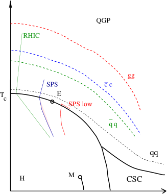
FIG. 1.: Schematic position of several zero binding lines on the QCD phase diagram, from SZ1.

Bound states in the QGP phase. The earliest QGP signal (suggested by one of us [1]) was the disappearance of familiar hadronic states, especially the vector ones – $\rho,\omega,\phi,J/\psi$ mesons – directly observable via dilepton experiments. It was suggested later that even small-size and deeply-bound states of charmonium such as $\eta_{c},J/\psi$ were expected to melt at $T\approx T_{c}$ [13, 14], so their absence was proposed to be a “golden signature” of the QGP. However, recent lattice works [15] using the Maximal Entropy Method (MEM) have found that charmonium states actually persists to at least $T\approx 2\,T_{c}$, and there are similar evidences about mesonic bound states made of light quarks as well [16]. As we will show below, this is in good agreement with independent lattice studies on the effective interaction potential between static sources in QGP . In SZ1 and now we argue that on top of familiar colorless hadronic states there should also be litterally hundreds of colored binary bound states, and for the singlet $gg$ pair (the most attractive channel) the region of binding should persist up to quite high temperature, i.e. $T\approx 4\,T_{c}$.

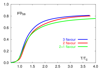
FIG. 2.: The pressure normalized to that of a gas of massless and noninteracting quasiparticles, or Stephan-Boltzmann value, versus the temperature $T/T_{c}$, from the lattice calculations by the Bielefeld group [18]. Different curves are for different numbers (masses) of the dynamical quarks.

The “high pressure puzzle” stems from Fig. 2 which shows a sample of lattice results for the QCD bulk pressure $p(T)$, normalized to Stephan-Boltzmann noninteracting value for each theory. At $T\approx 2\,T_{c}$ the pressure nearly saturates to 0.8 of that for massless noninteracting gas, $p_{SB}$.

This behaviour appears to be in contradiction with other lattice QCD works which found rather heavy quasiparticles, with masses (energies) e.g. of $M_{q,g}/T\sim 3$ at $T\approx 1.5-2\,T_{c}$ [17]. How could such heavy quasiparticles account for large pressures [18]? Substantial elliptic flow effects at RHIC [4] points also to a large pressure in the prompt phase at RHIC or at $T=(1-2)\,T_{c}$, so we do know it is there.

A similar discrepancy but now analytic and parametric, was found for CFT at parametrically large coupling. In our second paper [19] we argued that in this case the matter cannot be made of quasiparticles, which are again too heavy parametrically, but rather by their (much lighter) binary composites. The QGP picture we advocate is thus just a beginning of this parametric trend, with the intermediate running gauge coupling $\alpha_{s}\approx(1/2-1)$.

II Color forces in various binary channels

At $T>T_{c}$ there is no color confinement, and so the interaction is a Coulomb-like at small distances, with a Debye-type screening [20] at large distances. Both lattice data as we will use below and results from the AdS/CFT correspondence agree that these features of the potential carry to the strong coupling regime.

In this section we compare multiple binary colored channels , by using Casimir scaling for their relative strength. Its precise formulation can be made as follows. Let $A,B$ be the color representations of either the quark or gluon constituents. If they are in a colored bound state with overall color representation $D$, then their color interaction is proportional to 

$${\bf c}_{D}=\left(\vec{\lambda}_{A}\cdot\vec{\lambda}_{B}\right)_{D}=2\left({\bf C}(D)-{\bf C}(A)-{\bf C}(B)\right)\,\,\,,$$ (2)

where the ${\bf C}$’s are the pertinent Casimirs. For $SU(3)_{c}$ the Casimirs can be given in terms of the Dynkin index $(mn)$ of the representation $D$,

$${\bf C}(D)=m+n+\frac{1}{3}(m^{2}+n^{2}+mn)$$ (3)

In this section, we detail the color representations and the strength of the Coulomb interaction (2 in the bound states $\bf{gg}$, $\bf{qg}$ and $\bf{qq}$.

$\bf gg\,\,\,:$ Two gluons yield the sum of irreducible color representations $D={\bf 8}\otimes{\bf 8}={\bf 1}\oplus{\bf 8}_{S}\oplus{\bf 8}_{A}\oplus{\bf 10}_{S}\oplus\overline{\bf 10}_{A}\oplus{\bf 27}$. In terms of the Dynkin indices, the same irreducible decomposition yields $D=(00)\oplus(11)\oplus(11)\oplus(03)\oplus(30)\oplus(22)$. Thus (2) reduces to

$${\bf c}_{D}=\left(\vec{\lambda}_{8}\cdot\vec{\lambda}_{8}\right)_{D}=2\left({\bf C}(D)-2\,{\bf C}(8)\right)\,\,\,,$$ (4)

with ${\bf c}_{1}=-12$, ${\bf c}_{8}=-6$ (attractive) and ${\bf c}_{10}=0$ (inactive) and ${\bf c}_{27}=4$ (repulsive).

$\bf qg\,\,\,:$ A quark and a gluon yield the sum of irreducible color representations $D={\bf 3}\otimes{\bf 8}={\bf 3}\oplus{\bf 6}_{S}\oplus{\bf 15}$. In terms of the Dynkin indices, the same irreducible decomposition yields $D=(10)\oplus(02)\oplus(21)$. Thus (2) reduces to

$${\bf c}_{D}=\left(\vec{\lambda}_{3}\cdot\vec{\lambda}_{8}\right)_{D}=2\left({\bf C}(D)-4/3-3\right)\,\,\,,$$ (5)

with ${\bf c}_{3}=-6$, ${\bf c}_{6}=-2$ (attractive) and ${\bf c}_{15}=2$ (repulsive). A similar decomposition applies to the conjugate representation $\overline{\bf q}{\bf g}$ with $D=(01)\oplus(20)\oplus(12)$

$\bf\overline{q}q\,\,\,:$ A quark and an antiquark yield the sum of irreducible color representations $D=\overline{\bf 3}\otimes{\bf 3}={\bf 1}\oplus{\bf 8}$. In terms of the Dynkin indices, the same irreducible decomposition yields $D=(00)\oplus(11)$. Thus (2) reduces to

$${\bf c}_{D}=\left(\vec{\lambda}_{\overline{3}}\cdot\vec{\lambda}_{3}\right)_{D}=2\left({\bf C}(D)-8/3\right)\,\,\,,$$ (6)

with ${\bf c}_{1}=-16/3$ (attractive) and ${\bf c}_{8}=+2/3$ (repulsive).

$\bf{q}q$   . A two-quark state yield the sum of irreducible color representations $D={\bf 3}\otimes{\bf 3}=\overline{\bf 3}\oplus{\bf 6}$. In terms of the Dynkin indices, the same irreducible decomposition yields $D=(01)\oplus(20)$. Thus (2) reduces to

$${\bf c}_{D}=\left(\vec{\lambda}_{3}\cdot\vec{\lambda}_{3}\right)_{D}=2\left({\bf C}(D)-8/3\right)\,\,\,,$$ (7)

with ${\bf c}_{\overline{3}}=-8/3$ (attractive) and ${\bf c}_{6}=+4/3$ (repulsive).

Using a singlet $\bar{q}q$ as a standard benchmark (the only one studied extensively on the lattice), one can summarise the list of all attractive channels in Table I, indicating the relative strength of the Coulomb potential in a given color channel and the number of states. Even without the excited states to be discussed below, there is a total of 481 channels for two flavors (41 colorless), and 749 states (81 colorless) for three flavors.

III Bound states in strong Coulomb field

Before we analyze the relativistic two-body bound states for quarks and gluons, we go over the results for the simpler problems involving either a spin 0, spin 1/2 and spin 1 particle moving in a strong (color) Coulomb field, where the effect of color is treated as a Casimir rescaling of the Coulomb charge. Precession in color space can be treated but will be ignored through an “Abelianization” of the external field. The results for spin 0 and 1/2 are known from 1928 [21]. They are presented for completeness since they streamline our analysis for spin 1. A canonical application of the latter is that of a W boson bound to heavy Coulomb center.

channel	rep.	charge factor	no. of states
$gg$	1	9/4	$9_{s}$
$gg$	8	9/8	$9_{s}*16$
$qg+\bar{q}g$	3	9/8	$3_{c}*6_{s}*2*N_{f}$
$qg+\bar{q}g$	6	3/8	$6_{c}*6_{s}*2*N_{f}$
$\bar{q}q$	1	1	$8_{s}*N_{f}^{2}$
$qq+\bar{q}\bar{q}$	3	1/2	$4_{s}*3_{c}*2*N_{f}^{2}$

TABLE I.: Binary attractive channels discussed in this work, the subscripts s,c,f mean spin,color and flavor, $N_{f}=3$ is the number of relevant flavors.

A Spin 0

For a scalar particle the Klein-Gordon equation

$$\left((E-gV)^{2}-m^{2}+\vec{\vec{\partial}}^{2}\right)\,\Phi=0$$ (8)

should be used. This equation was analyzed for a Coulomb potential $gV=-\alpha/r$ in [21] with the energy spectrum

$${E(n_{r},l)\over m}\,\left(1+{\alpha^{2}\over(n_{r}+\sqrt{(l+1/2)^{2}-\alpha^{2}})^{2}}\right)^{1/2}=1$$ (9)

Taking the lowest level to be $n_{r}=1,l=0$ as an example, one finds that $\alpha=1/2$ is a critical value for this equation. Although the binding is at this point finite and even not large, $E(1,0)/m=\sqrt{4/5}$, something new is obviously happening at this critical coupling because the square root (in the denominator) goes complex.

What happens is that the particle starts falling towards the center. Indeed, ignoring at small $r$ all terms except the $V^{2}$ term one finds that the radial equation is

$$R^{\prime\prime}+{2\over r}R^{\prime}+{\alpha^{2}\over r^{2}}R=0$$ (10)

which at small $r$ has a general solution

$$R=Ar^{s_{+}}+Br^{s_{-}},\hskip 14.22636pts_{\pm}=-1/2\pm\sqrt{1/4-\alpha^{2}}$$ (11)

that for $\alpha\rightarrow 1/2$ is just $1/r^{1/2}$. At the critical coupling $both$ solutions have the same (singular) behavior at small $r$. For $\alpha>1/2$ the falling starts, as one sees from the complex (oscillating) solutions.

In the CFT theory with fixed (non-running) coupling constant, nothing can prevent the particle from falling to arbitrary small r as soon as $\alpha>1/2$ . In contrast, in QCD the coupling runs, $\alpha(r)\approx 1/{\rm ln}(1/r\Lambda_{QCD})$, so that at small enough distances the coupling gets less than critical and the falling stops. In [22] a crude model of a regularized Coulomb field was used, producing the same effect. Our arguments show that asymptotic freedom would be in principle enough. However, the wave function at the origin is changing dramatically at $\alpha\approx 1/2$ and in view of that we performed an additional study of the Klein-Gordon problem with a Coulomb+quasi-local potential in the Appendix.

The falling onto the center happens for any spin of the particle, only the value for the critical coupling is different. We now proceed to show that.

B Spin $\frac{1}{2}$

The squared Dirac equation for a massive spinor ${\bf\Psi}$ reads

$$\left(\Box+m^{2}-\frac{g}{2}\,\sigma_{\mu\nu}\,F^{\mu\nu}\right)\,{\bf\Psi}=0\,\,,$$ (12)

with $\sigma_{\mu\nu}=i[\gamma_{\mu},\gamma_{\nu}]/2$ and $F^{\mu\nu}$ the external background field. In the chiral basis, (12) simplifies

$$\left((\Box+m^{2})+2g\,\vec{\bf S}\cdot(\vec{\bf B}\mp i\vec{\bf E})\right){\bf\Psi}_{\pm}=0\,\,,$$ (13)

where the spin operator is Lie-algebra valued,

$$\left[{\bf S}^{a},{\bf S}^{b}\right]=if^{abc}\,{\bf S}^{c}$$ (14)

The magnetic contribution in (12) is standard. The electric contribution is complex  and is reminiscent of a Bohm-Aharanov effect.

The relativistic Coulomb problem stemming from (12) for each of the two stationary spin components reads

$$\left((E+\frac{g^{2}}{r})^{2}-m^{2}+\frac{d^{2}}{dr^{2}}+\frac{2}{r}\frac{d}{dr}-\frac{{\vec{\bf L}}^{2}}{r^{2}}-\frac{2ig^{2}}{r^{2}}\vec{\bf S}\cdot\hat{r}\right){\bf\Psi}=0\,\,.$$ (15)

(16)

the solutions to (16) are naturally sought in terms of spinor spherical harmonics [23]

$${\bf\Psi}^{a}_{JML}=\sum_{b}\left(\matrix{J&L&\frac{1}{2}\cr-M&(M-b)&b\cr}\right)\,{\bf e}_{b}^{a}Y_{L}^{M-b}\,\,,$$ (17)

with the bracket a conventional Clebsch-Gordon coefficient restricting the values of $L$ and $a,b=\pm 1/2$. In this representation the spinors are just ${\bf e}^{a}_{b}=\delta^{ab}$, and (17) is an eigenstate of ${\bf J}^{2}$, ${\bf J}_{3}$ and ${\bf L}^{2}$ with eigenvalues $J(J+1)$, $-M$ and $L(L+1)$ respectively. In the basis (17) the spin operator ${\bf S}\cdot\hat{r}$ is off-diagonal

$${\bf S}\cdot\hat{r}=\left(\matrix{0&-\frac{1}{2}\cr-\frac{1}{2}&0\cr}\right)\,\,.$$ (18)

Using the spinor spherical harmonics (17) in (16) through the expansion

$${\bf{\Psi}}=\sum_{a}\,{\bf\Psi}^{a}_{JML}\,{\bf R}^{a}$$ (19)

for fixed $JM$ and (18) we obtain the $2\times 2$ matrix equation for the radial function ${\bf R}$

$$\left((E+\frac{g^{2}}{r})^{2}-m^{2}+\frac{d^{2}}{dr^{2}}+\frac{2}{r}\frac{d}{dr}-\frac{J(J+1)+{\bf C}}{r^{2}}\right)\,{\bf R}=0$$ (20)

(21)

with

$${\bf C}=\left(\matrix{\frac{1}{4}-(J+\frac{1}{2})&-ig^{2}\cr-ig^{2}&\frac{1}{4}+(J+\frac{1}{2})\cr}\right)\,\,.$$ (22)

The eigenvalues of ${\bf C}$ are

$$\lambda_{\pm\frac{1}{2}}=\frac{1}{4}\pm\sqrt{(J+\frac{1}{2})^{2}-g^{4}}\,\,.$$ (23)

In terms of (23) the eigenvalue equation (21) becomes diagonal for the rotated ${\bf R}$. Defining $\epsilon=\sqrt{m^{2}-E^{2}}$ and $r=x/2\epsilon$ and ${\bf R}=2\epsilon\,{\bf U}/\sqrt{x}$ yield (21) in the diagonal basis in the form

$$x{\bf U}^{\prime\prime}+{\bf U}^{\prime}+\left(\alpha-\frac{x}{4}-\frac{\beta^{2}}{4x}\right)\,{\bf U}=0$$ (24)

with

$$\alpha= g^{2}\frac{E}{\epsilon}$$ (25)

$$\left(\frac{\beta}{2}\right)^{2}= (J+\frac{1}{2})^{2}+\lambda_{\pm\frac{1}{2}}-g^{4}\,\,.$$ (26)

The equation (24) is a standard hypergeometric equation. The bound state solutions with $|E|<m$ are Laguerre polynomials for

$$\alpha=n+\frac{1}{2}+\frac{\beta}{2}$$ (27)

which is the quantization condition with integer $n$ referring to the nodal number of the wavefunction as opposed to the radial quantum number $n_{r}$ used above. Unwinding (27) in terms of (26) yields the spectra for the relativistic spin $1/2$ particles/antiparticles

$$\frac{E}{m}\left(1+\frac{g^{4}}{(n+\frac{1}{2}+\frac{\beta}{2})}\right)^{1/2}=\pm 1$$ (28)

with (26) given explicitly by

$$\frac{\beta}{2}=\left|\sqrt{(J+\frac{1}{2})^{2}-g^{4}}\mp\frac{1}{2}\right|\,\,,$$ (29)

after using (23). This result is in agreement with the original result established in [21]. Note that for scalars it agrees with the semiclassical results we used earlier.

C Spin 1

The same analysis performed above can be carried out for the gauge-independent part of the wavefunction. Indeed, let us first consider a massless gluon in an arbitrary covariant background field gauge. The equation of motion is standard and reads

$$\left(\Box\,\delta_{\mu\nu}-(1-\frac{1}{\xi})\,\nabla_{\mu}\,\nabla_{\nu}-2ig\,F_{\mu\nu}\right)\,{\bf a}^{\nu}=0$$ (30)

which simplifies for Feynman gauge $\xi=1$ to

$$\left(\Box\,\delta_{\mu\nu}-2ig\,F_{\mu\nu}\right)\,{\bf a}^{\nu}=0$$ (31)

with $\nabla_{\mu}{\bf a}^{\mu}=0$. The gluon in (31) has two physical polarizations, the longitudinal and time-like ones being gauge artifacts. Generically, we can decompose the gluon along its polarizations ${\bf a}^{\mu}={\bf e}^{\mu}_{a}{\bf\Psi}^{a}$, and rewrite (31) in the form

$$\left(\Box+\frac{g}{2}\Sigma^{\mu\nu}\,F_{\mu\nu}\right)\,{\bf\Psi}=0$$ (32)

with $i\Sigma_{\mu\nu}/4={\bf e}^{T}_{\mu}{\bf e}_{\nu}$. This result is reminiscent of the massless spin $\frac{1}{2}$ equation (12) if we were to interpret $\Sigma_{\mu\nu}$ as the spin-operator of the gluon in the polarization space .

For massive gluons the pertinent equation is a variant of the Proca equation extensively used in the litterature. Here instead, we proceed by analogy with the spin 1/2 case. In the polarization space the equation of motion for spin 1 is just (the g-factor is now 1 instead of 2)

$$\left((\Box+m^{2})+g\,\vec{\bf S}\cdot(\vec{\bf B}-i\vec{\bf E})\right){\bf\Psi}=0\,\,,$$ (33)

which is readily checked from the path integral approach in the first quantization (see also below). Note that (33) is a $3\times 3$ matrix equation for one longitudinal and two transverse polarizations. For spin 1 gluons, ${\bf S}^{A\,ab}=i\epsilon^{Aab}$. In an external electric gluon field, (33) reduces to

$$(\Box+m^{2})\,\vec{\bf\Psi}+g\,(\vec{\bf E}\times\,\vec{\bf\Psi})=0\,\,,$$ (34)

which shows that the electric field causes the polarization to precess in the relativistic equation. To solve (33) in a Coulomb field ${\bf E}=-g\hat{r}/r^{2}$ we use exactly the same method discussed for spin $\frac{1}{2}$ except for the use of vector instead of spinor spherical harmonics,

$${\bf\Psi}^{a}_{JML}=\sum_{b}\left(\matrix{J&L&1\cr-M&(M-b)&b\cr}\right)\,{\bf e}_{b}^{a}\,Y_{L}^{M-b}$$ (35)

with $a,b=0,\pm 1$. In this representation the three polarizations are chosen real with again ${\bf e}^{a}_{b}=\delta^{ab}$. A rerun of the precedent arguments show that (21) holds for spin 1 in a $3\times 3$ matrix form with the substitution

$${\bf C}=\left(\matrix{1-(2J+1)&-ig^{2}\sqrt{\frac{J+1}{2J+1}}&0\cr-ig^{2}\sqrt{\frac{J+1}{2J+1}}&0&-ig^{2}\sqrt{\frac{J}{2J+1}}\cr 0&-ig^{2}\sqrt{\frac{J}{2J+1}}&1+(2J+1)\cr}\right)\,\,,$$ (36)

for $J\neq 0$. The case $J=0$ is special since ${\bf C}={\rm diag}(0,0,2)$. The eigenvalues of ${\bf C}$ are solution to a cubic (Cardano) equation

$$\lambda^{3}+2\lambda^{2}+\lambda(1-(2J+1)^{2}+g^{4})+2g^{4}=0\,\,.$$ (37)

The solutions are all real since the polynomial discrimant of (37) is negative [24]. This is expected since the gluon evolution operator is hermitean. The explicit solutions to (37) are [24]

$$\lambda_{a}=2\sqrt{-Q}\,{\rm cos}\left(\frac{\theta+2\pi\,a}{3}\right)-\frac{2}{3}$$ (38)

with ${\rm cos}\,\theta=R/\sqrt{-Q^{3}}$ and

$$Q= \frac{1}{3}(1-(2J+1)^{2}+g^{4})-\frac{4}{9}$$ (39)

$$R= \frac{1}{3}(1-(2J+1)^{2}+g^{4})-g^{4}-\frac{8}{27}\,\,\,.$$ (40)

The corresponding spectrum for spin 1 particle is again of the type

$$\frac{E}{m}\left(1+\frac{g^{4}}{(n+\frac{1}{2}+\frac{\beta}{2})}\right)^{1/2}=\pm 1$$ (41)

with

$$\left(\frac{\beta}{2}\right)^{2}=(J+\frac{1}{2})^{2}+\lambda_{0,\pm 1}-g^{4}\,\,.$$ (42)

The case $J=0$ is special and yields $\lambda=(0,0,2)$. (Thus one can see that the minimal critical coupling is $\alpha=1/2$, as for spinless case.) Much like the quarks and scalars, the gluons fall onto the center at a critical coupling which is now set by the branch point of not only (42) but also (38).

IV A two-body bound state problem

A Generalities

Non-relativistically, the problem of two bodies (e.g. positronium) is readily reduced to a single one body problem (hydrogen atom) by a simple adjustment of the particle mass. Relativistically this is more subtle.

Let us start with two spinless particles, obeying two separate Klein Gordon equations. Making use of the fact that in the CM the two momenta are equal and opposite $\vec{p}=\vec{p}{(1)}=-\vec{p}{(2)}$ one can eliminate the relative energy $p_{0}{(1)}-p_{0}{(2)}$ for the total energy $E=p_{0}{(1)}+p_{0}{(2)}$. The resulting relations

$$\kappa^{2}-\vec{p}^{2}=0$$ (43)

$$\kappa^{2}=(E/2)^{2}-(m_{1}^{2}+m_{2}^{2})/2+{(m_{1}^{2}-m_{2}^{2})^{2}\over 4E^{2}}$$ (44)

can be used as the KG equation for two particles with different masses. The KG simplifies for equal masses, when the last term drops out. Fortunately this is is approximately true for our problem, since for $T$ in the region of interest the quasiparticle mass difference is relatively small even for $qg$ states.

The quantization follows from the canonical substitution $E\rightarrow-i\partial_{t}-V$, $\vec{p}\rightarrow-i\vec{\partial}-g\vec{A}$. The magnetic effects through $\vec{A}$, are comparable to the electric effects for $v\approx 1$.

FIG. 3.: Classical motion of two mutually attracting charges. If the field propagation is instantaneous, a partner of a particle P is at the “antipode” point A. However if particles move relativistically and the electromagnetic field travels at light speeds, the particle P sees a field from the earlier position B (drawn for counterclockwise rotation).

The next problem is to understand what exactly is the 4 potential $(V,\vec{A})$ in this equation. That is of course the field at one particle (say P in Fig. 3) due to the other one. Non-relativistically the particle speed is negligible compared to the speed of light, so one can safely place the other particle at the opposite point (say A in Fig. 3).

Including retardation, one classically expects the field to emanate from B instead of A. The retarded position B is simply determined by the condition that the travel time from B to A equals the time it takes light from B to P, that is $(AB)/v=(PB)/c$. In the ultrarelativistic case $v=c$ and one gets a simple equation for the maximal retardation angle $a$,

$$a=\sqrt{2+2\,{\rm cos}\,a}$$ (45)

with a root at $a=1.48$. The retardation angle is about $85^{0}$ which is rather large.

The classical description is oversimplified, and in fact quantum theory allows for field propagation with any speed, not just c. It demands a convolution of the path (current) with the quantum propagator of a photon (gluon). At this point, it may appear that all hope to keep a potential model is lost and a retreat to a full quantum field theory treatment is inevitable.

This is indeed the case for intermediate coupling $\alpha\approx 1$, but when it gets stronger one can again claim some virtue in a potential-based approach. Our argument presented in [19] resulted in the conclusion that the effective photon (gluon) speed is not the usual speed of light but larger, by a parameter ${}^{4}\sqrt{\lambda}\gg 1$ (where as usual $\lambda=g^{2}N_{c}$). Thus the field is still dominated by the emission at the “antipode” that is point A instead of B.

The magnetic effects are the usual current-current interactions, present for spinless particles as well, plus those induced by (gluo) magnetic moments related with particle spins, plus their combination (spin-orbit). The spin effects were argued to be small, see [22, 19].

For an extensive review of the known results on how one can reduce a 2-body relativistic Dirac problem to that of a potential problem we refer to [25]. Here we just note as in [19] that in the QGP the quark mass is a “chiral mass”, so the derivation of the effective single-body Dirac equation in this case would be a priori different from the one discussed in [25].

B Relativistic Two-Body Bound States

In this section we illustrate the derivation of the relativistic two-body bound states between ${\bf qq}$, ${\bf gg}$ and ${\bf qg}$ in QCD by considering the simpler problem in relativistic QED in both the first and second quantized form. The generalization to QCD is staightforward in the canonical quantization approach i.e. $A_{0}=0$ gauge.

1 Second Quantization

Consider two massive relativistic electrons with Dirac spinors $\Psi_{a}$ and $a=1,2$

$${\cal L}=\sum_{a=1,2}\,\overline{{\bf\Psi}}_{a}\,(i\hbox to0.0pt{/\hss}{\nabla}-{\bf m}_{a})\,{\bf\Psi}_{a}-\frac{1}{4}F_{\mu\nu}F^{\mu\nu}\,\,.$$ (46)

Canonical quantization of (46) yields the hamiltonian density

$${\cal H}={\cal H}_{F}+\frac{1}{2}({\vec{\bf E}}^{2}+{\vec{\bf B}}^{2})-\vec{J}\cdot\vec{A}+(J_{0}-\vec{\partial}\cdot{\vec{\bf E}})\,A_{0}\,\,$$ (47)

with ${\cal H}_{F}$ the free fermion hamiltonian density and

$$J^{\mu}=g\,\sum_{a=1,2}\,\overline{\bf\Psi}_{a}\gamma^{\mu}{\bf\Psi}_{a}\,\,.$$ (48)

The coefficient of $A_{0}$ (constraint) is Gauss law. The latter is resolved in terms of the Coulomb potential

$$\vec{\bf E}_{L}=-\frac{1}{2}\,J^{0}\,\partial^{-2}\,J^{0}\,\,.$$ (49)

Ampere’s law follows from the equation of motion for the transverse part of the electric field

$$\dot{\vec{\bf E}}_{T}=-i\left[{\bf H}\,,\,\vec{\bf E}_{T}\right]=\partial^{2}\,{\vec{A}}_{T}-\vec{J}\,\,.$$ (50)

For stationary (bound) states $\vec{A}_{T}=(1/\partial^{2})\vec{J}$ and the hamiltonian density (47) simplifies

$${\cal H}={\cal H}_{F}+\frac{1}{2}\vec{\bf E}_{L}^{2}-\frac{1}{2}\vec{\bf B}^{2}\,\,,$$ (51)

which is the same as

$${\cal H}= {\bf{\Psi}}^{\dagger}\left(i\vec{\alpha}\cdot\vec{\partial}\,+\beta\,{\bf m}\right){\bf\Psi}$$ (54)

$$+\frac{g^{2}}{2}{\bf\Psi}^{\dagger}{\bf\Psi}\frac{-1}{\partial^{2}}{\bf\Psi}^{\dagger}{\bf\Psi}$$

$$-\frac{g^{2}}{2}{\bf\Psi}^{\dagger}i\alpha^{i}{\bf\Psi}\frac{-1}{\partial^{2}}(\delta^{ij}-\frac{\partial^{i}\partial^{j}}{\partial^{2}}){\bf\Psi}^{\dagger}i\alpha^{j}{\bf\Psi}\,\,,$$

This form is standard, with the Coulomb (Gauss law) and the current-current (Ampere’s law) interaction. For two particles the spin effects are encoded in the spinors ${\bf\Psi}$ along with the particle-antiparticle content. They may be unravelled non-relativistically using a Foldy-Woutuhysen transformation.

2 First Quantization

Perhaps a more transparent way to address the spin effects in the presence of gauge fields when the particle-antiparticle content is not dominant, is to use the first quantized form of the same problem. For that it is best to choose the einbein formulation [26] in the rest frame. For two gauge coupled particles it reads

$${\cal L}= -\frac{V_{a}}{2}(1-\dot{\vec{x}}^{2}_{a})-\frac{{\bf m}_{a}^{2}}{2V_{a}}+g\,A^{0}_{a}-g\dot{\vec{x}}_{a}\cdot{\vec{A}}_{a}$$ (56)

$$+\frac{1}{2}(\vec{\bf E}^{2}-\vec{\bf B}^{2})+\frac{g}{V_{a}}\vec{\bf S}_{a}\cdot(\vec{\bf B}_{a}\mp i\vec{\bf E}_{a})$$

where $a=1,2$ is summed over throughout unless indicated otherwise, and $A_{a}=A(x_{a})$ and similarly for the fields. The einbeins are denoted by $V_{a}$. They will be considered as Lagrange multipliers at the end and fixed by minimizing the energy. The $\mp$ refers to particle-antiparticle.

We note that while the potentials couple canonically to the currents, the spin couples canonically to the magnetic field but has an imaginary coupling to the electric field in Minkowski space, a situation reminiscent of Berry phases. Indeed, canonical quantization of (56) yields the momenta (only the upper sign is retained from now on)

$$\vec{p}_{a}= V_{a}\,\dot{\vec{x}}_{a}-g\vec{A}_{a}$$ (57)

$$\vec{\Pi}(x)= \vec{\bf E}(x)-\frac{ig}{V_{a}}\,\vec{\bf S}_{a}\,\delta(\vec{x}-\vec{x}_{a})\,\,.$$ (58)

The canonical momentum $\vec{\Pi}$ has a complex shift due to the spin of the particle in contrast to the second quantized analysis. By insisting that (58) are canonical, we conclude that the energy spectrum is shifted by the Berry phase.

The canonical Hamiltonian following from (56) after resolving Gauss law reads

$${\cal H}= \frac{1}{2V_{a}}(\vec{p}^{2}_{a}+g\vec{A}_{a})^{2}+\frac{{\bf m}_{a}^{2}}{2V_{a}}-\frac{V_{a}}{2}$$ (61)

$$-g\frac{\vec{\bf S}_{a}}{V_{a}}\cdot(\vec{\bf B}_{a}-i\vec{\Pi}_{La}-i\vec{\Pi}_{Ta})$$

$$+\frac{1}{2}\vec{\Pi}^{2}_{L}+\frac{1}{2}(\Pi_{T}^{2}+{\vec{\bf B}}^{2})^{2}-\frac{1}{2V_{a}^{2}}\vec{\bf S}_{a}\cdot\vec{\bf S}_{a}\,\delta(\vec{0})$$

with

$$\vec{\Pi}_{L}(x)=-g\frac{1}{\partial^{2}}\vec{\partial}\,\sum_{a}\delta(\vec{x}-\vec{x}_{a})\,\,,$$ (62)

with the summation over $a$ shown explicitly.

For stationary states the equation of motions can be used to solve for $\vec{A}_{T}$ and therefore for $\vec{\Pi}_{T}$ and $\vec{\bf B}$ through Ampere’s and Lenz’s law. In particular,

$$\vec{A}_{T}(x)= -\frac{1}{V_{a}\partial^{2}}(\vec{p}_{a}+g\vec{A}_{Ta})\,\delta(\vec{x}-\vec{x}_{a})$$ (64)

$$-\frac{1}{V_{a}\partial^{2}}\,g(\vec{\bf S}_{a}\times\vec{\partial})\,\delta(\vec{x}-\vec{x}_{a})\,\,.$$

Noting that the momenta scales with the einbeins as $\Pi_{L}\approx V^{0}$ and that $\Pi_{T}\approx{\bf B}\approx 1/V$, it follows that for stationary states the hamiltonian simplifies to order ${\cal O}(1/{V^{2}})$, i.e.

$${\cal H}\approx\frac{1}{2V_{a}}\left(\vec{p}^{2}_{a}+{\bf m}_{a}^{2}+V^{2}_{a}+2ig\vec{\bf S}_{a}\cdot\vec{\Pi}_{La}\right)+\frac{1}{2}{\vec{\Pi}^{2}_{L}}\,\,.$$ (65)

The expansion in $1/V^{2}$ is justified in the non-relativistic limit since $V\approx{\bf m}$ and the ultrarelativistic limit since $V\approx\gamma{\bf m}$ (here $\gamma$ is the Lorentz contraction factor). Indeed, the extrema in $V$ of the total hamiltonian ${\bf H}$ associated to (65) are complex and read

$$V_{a}=\sqrt{p_{a}^{2}+{\bf m}_{a}^{2}+2ig\,\vec{\bf S}_{a}\cdot\vec{\Pi}_{La}}\,\,.$$ (66)

in particular $V\approx\gamma{\bf m}$ as asserted. For a pair of identical particles ${\bf m}_{1}={\bf m}_{2}$ in their center of mass frame $\vec{p}_{1}=-\vec{p}_{2}=\vec{p}$, (65) and (66) yield

$$\frac{1}{4}\left({\bf H}+\frac{g^{2}}{x_{12}}\right)^{2}\approx\vec{p}^{2}+{\bf m}^{2}-2ig^{2}(\vec{\bf S}_{1}-\vec{\bf S}_{2})\cdot\vec{\partial}\,\frac{1}{x_{12}}$$ (67)

after absorbing the Coulomb self-energy corrections in the masse ${\bf m}$ . (67) gives a spectrum analogous to the one described in the background field section except for the fact that now each of the two particles carry its own spin in the center of mass frame. Spin-orbit and spin-spin effects are obtained by carrying the expansion a step further in $1/V$ in ${\cal H}$.

V Bound states in static effective potentials

Studies of effective potentials in lattice QCD have a long history. Their $T=0$ version was first obtained in the classic paper by M. Creutz who first found confinement on the lattice in 1979. The first finite-T results have shown Debye screening, in agreement with theoretical expectations [1]. These static potentials lead to early conclusions [13, 14] that all states, even the lowest $\bar{c}c$ states and $\eta_{c},J/\psi$, melt at $T\approx T_{c}$. As we already mentioned in the introduction, these conclusions contradict the recent MEM analysis of the correlators which indicate that charmonium states stubbornly persist till about $2T_{c}$.

On theoretical grounds, it has been repeatedly argued (see e.g. [27]) that close to $T_{c}$ the Debye mass is low enough to allow the color charge to run to rather large values. If so, the binding of many states must occur, as it was shown in our letter [3].

Recently in a number of publications, the Bielefeld group had reanalyzed the effective static potentials. One of the key point missed in previous works is that the expectations values obtained from thermal average are by definition the free energy $F$, related with the energy E by the standard thermodynamical relation

$$E=F-TS\,\,.$$ (68)

So in order to understand the potential $energy$ one has to remove the entropy part first. The subtraction results in in much deeper potentials, which (as we will show below) readily bind heavy (and light) quarks.

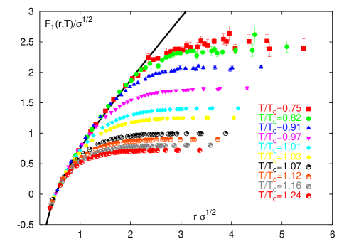
FIG. 4.: Heavy quark free energies in the singlet channel for 2-flavors of dynamical quarks at a quark mass of $m/T=0.40$ on $16^{3}\times 4$ lattices renormalized to the zero-$T$ potential obtained from [28].

A set of potentials obtained by the Bielefeld group is shown in Fig.4. The strength of the effective interaction can be characterize by a combination, called a screening function,

$$S_{1}(r,T)=-\frac{3}{4}r(F_{1}(r,T)-F_{1}(\infty,T))$$ (69)

where the subscript 1 refers to the color singlet channel and the 3/4 removes the Casimir for $\bar{q}q$ representation, so that $S_{1}$ is in a way just an effective gauge coupling $\alpha_{s}$. A sample of these effective gauge couplings are plotted in Fig. 5. The logarithmic plot shows exponential decrease at large r, while the non-logarithmic plot shows a decrease toward small $r$ due to asymptotic freedom. The maximum at $rT\approx 1/2$ indicates that the effective Coulomb coupling at $T_{c}$ is $\alpha_{\rm eff}\approx 4/3S_{1}\approx 1/2$, right in the ballpark used in [22]. One should also note that the strength is even larger below $T_{c}$, where it is related with confinement at the string breaking point. Finally, we note the surprisingly monotonous behavior through the phase transition point, due to the fact that at $T>T_{c}$ the static charge continues to be screened by a single light quark, like in a heavy-light (B-like) meson below $T_{c}$.

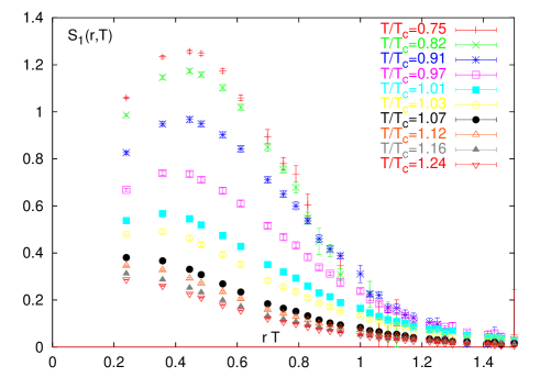
FIG. 5.: The color singlet screening function, from [28].

The effective quark mass, or a constant value of the potential, was subtracted out: it plays an important role in what follows.

We have parameterized these Bielefeld data by the following expression (here and below all dimensions are set up by $T_{c}$, e.g. $T$ means $T/T_{c}$ and $r$ is $rT_{c}$)

$$F_{1}(T,r)=1.5-1.1(T-1)^{1/2}-{4\over 3r}{e^{(-2Tr)}\over{\rm ln\,}(1/r+3T)}$$ (70)

and then extracted from it the potential energy using $E_{1}=F_{1}-TdF_{1}/dT$.

Furthermore, an appropriate normalization of the potential to be used for the bound state analysis is its decay at infinity. We use $V(T,r)=E_{1}(T,r)-E_{1}(T,r=\infty)$. (Non-relativistically, the constant part can be added to a mass.) The resulting potentials are plotted in Fig. 6

Our next next step after extracting the lattice potentials 6 is to use them in a Schrodinger (or appropriate relativistic) equation and solve for the bound states. A sample of the results obtained using the Klein-Gordon equation with this potential is plotted in Fig. 7. We used a charm quark mass of $1.5\,GeV$ and an effective gluon mass of $0.6\,GeV$: the results are not very sensitive to it.

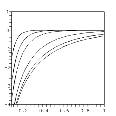
FIG. 6.: The static potentials $V(T,r)$ as a function of the distance $rT_{c}$. The values of temperature used are $T=1.,1.2,1.4,2.,4.,6.,10.T_{c}$, from right to left.

One can see that charmonium remains bound to about $T=2.7T_{c}$. It is in fact completely consistent with lattice observations [15] using MEM. The fact that the state is traced only to $T<2T_{c}$ is completely understandable, as for $2<T/T_{c}<2.7$ it is so weakly bound that the size of the state may exceed the size of the lattice and could not possible be seen. Note that at all $T$ the charmonium binding remains rather small, and so the nonrelativistic treatment of charmonium would be completely justified. A similar conclusion would be reached for light $\bar{q}q$ pairs.

This is not the case for the gluonic singlet $gg$ state, which has a color charge larger by the ratio $9/4$. We found that the same potential in this case leads to much larger binding, reaching up to 40 percent of the total mass at $T=T_{c}$. There is no question that the relativistic treatment is indeed needed here.

We have also looked for $l=1$ states in this potential, which we only found for the most attractive singlet $gg$ state. Those reache their zero binding at $T=1.0805\,T_{c}$. Another next-shell state is an $l=0,n=2$ state, which exists till $T<1.205\,T_{c}$. (Those states are not included in the calculation of the thermodynamical quantities at the end of the paper.)

VI Relativistic corrections and instanton molecules

A Relativistic corrections

The lattice potentials used above were evaluated for static charges without spin, therefore it does not include effects proportional to particle velocities and/or spins. Although we used a relativistic KG equation, we see that $\bar{q}q$ (and even the most attractive color singlet $gg$ state) are not bound nearly enough as to become massless. On the other hand, we know that the lowest $\bar{q}q$ states, the pion-sigma multiplet, must do so at $T=T_{c}$. It means that something is missing in the interaction. We will discuss those missing effects in the next section.

The first relativistic effect, already discussed in Ref. [22], is the velocity-velocity force due to magnetic interaction (Ampere’s law in the classical treatment). This corresponds to a substitution of the effective Coulomb coupling by

$$\alpha\rightarrow\alpha(1-\vec{\beta}_{1}\vec{\beta}_{2})$$ (71)

where $\beta_{i}$ are velocities (in units of $c$) of both charges. In the center of mass the velocities are always opposite, so the the effective coupling always increases.

We have estimated the mean velocity squared by using the equation itself

$$<v^{2}>=\int dr\chi^{2}(r)\left(1-\left(\frac{2M}{E-V(r)}\right)^{2}\right)$$ (72)

where the wave function is appropriately normalized. This yields $<v^{2}>=.12$ for light quarks at $T/T_{c}=1.05$. If we plug this correction back into the potential, assuming it scales as $(1+<v^{2}>)$ as a whole  we get larger binding (squares in Fig. 7). With this relativistic correction included, at $T\approx T_{c}$ the light quarks become relativistic and about as bound as the charmed quarks, with mean velocity of about 1/3.

Although we do not yet see how very relativistic motion may come about, we will do so in the next section. In anticipation of that, let us show here what can be a maximal effect of the the relativistic correction under consideration. If the particle velocity becomes the speed of light, a correction under consideration effectively doubles the coupling, putting it at $T\approx T_{c}$ to be $\alpha_{\rm eff}\approx 1$. If we simply double the effective potential as a whole, the binding increases significantly. The result is shown by a single square in Fig. 7(a), and at $T=T_{c}$ the binding reaches about 1/4 of the total mass. Even larger effect is seen in the particle density at the origin. As shown in Fig. 7(b) it increases by about an order of magnitude.

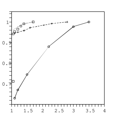
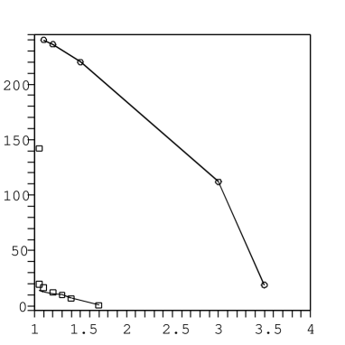
FIG. 7.: (a) The energy of the bound state $E$ (in units of the total mass 2M) versus the temperature $T/T_{c}$ using the lattice effective potential $V(T,r)$, for charmonium (crosses and dashed line), singlet light quarks $\bar{q}q$ (solid line) and $gg$ (solid line with circles). A set of squares show the relativistic correction to light quark, a single square at $T=1.05T_{c}$ is for $\bar{q}q$ with twice the coupling, which is the maximal possible relativistic correction. (b) The density at the origin $|\psi(0)|^{2}/T_{c}^{3}$ of the bound states versus the temperature $T/T_{c}$ in the lattice effective potential $V(T,r)$, for singlet light quarks $\bar{q}q$ and $gg$ (upper and lower lines with circles). A single square at $T=1.05T_{c}$ is for $\bar{q}q$ with twice the coupling.

B Interaction induced by the instanton molecules

We have seen in the preceding section that relativistic effects proportional to velocities make all states significantly more bound and dense at $T\rightarrow T_{c}$: but still these effects are too weak to bring the total energy of the lowest $\bar{q}q$ to zero, as is required for sigma mesons to trigger a phase transition at $T=T_{c}$ coming from above on the temperature axis.

As discussed in BLRS paper [22], the missing element is a quasi-local interaction induced by the instanton-antiinstanton molecules, the lowest clusters of zero total topological charge allowed in the chirally restored phase (see [29] for a review).

In this paper we will not try to estimate the coupling from first principle but instead adopt a purely phenomenological approach. For the local 4-fermion interaction with the coupling constant $G$ the energy shift is given simply by

$$\delta E=-G|\psi(0)|^{2}\,\,.$$ (73)

Here we will tune the magnitude of the effective 4-fermion coupling $G_{4q}$ so that the pion-sigma multiplet gets massless (and then tachyonic) exactly at $T=T_{c}$.

With $|\delta E|=0.92M_{q}\approx 1.3{\rm GeV}$ and $|\psi(0)|^{2}\sim 350T_{c}^{3}$, after the relativistic correction is included, one needs $G\approx 1.5{\rm GeV}^{2}$, which is in the expected ballpark  If the relativistic correction would not be there, the value of $|\psi(0)|^{2}$ would be an order of magnitude smaller, see Fig. 7(b).

The remaining problem is what happens in the glueball ($gg$ singlet) channel, where we expect the interaction with instantons to be even stronger than with quarks. Indeed, the instantons are classical objects made of gluon field, thus their interaction with gluons would be proportional to the action $O(S\approx 8\pi^{2}/g^{2})$ which is expected to be about 10 times stronger than ’t Hooft’s interaction with quarks. If this is the case, the s-wave glueball state gets tachyonic already at some finite $T$ above $T_{c}$.

VII Contribution of the bound states to thermodynamical quantities

A The contribution of the quasiparticles

Let us start with the papers by Peshier et al [30] and Levai and Heinz [31] who used a simple quasiparticle gas model, deducing what properties the $q,g$ quasiparticles should have in order to reproduce the lattice data of the pressure  $p(T)$. Assuming the usual dispersion relation $\omega^{2}=p^{2}+M(T)^{2}$, one has to deal with the $T$-dependent of the masses. For example, for pure glue it is possible to reproduce $p(T)$ by assuming $M_{g}(T)$. The qualitative behavior found in [31] at high $T$ is about linear and rising, as expected perturbatively [20]. For $T=(1.3-3)\,T_{c}$ it is about constant, with a rise towards $T_{c}$, an indication of the onset of confinement.

Although these features are qualitatively consistent with the direct measurements [17], they are not quantitatively. For $N_{f}=2$ the expected masses at $T=1.5\,T_{c}$ (close to their minimum) from [31] are

$$M_{g}\approx 420\,{\rm MeV}\,\qquad M_{q}\approx 300\,{\rm MeV}\,\,.$$ (74)

However direct studies by Karsch and Laerman found heavier ones

$$M_{g}\approx 540\,{\rm MeV}\,\qquad M_{q}\approx 620\,{\rm MeV}\,\,.$$ (75)

If the reader is not impressed by this difference, let us mention that the corresponding Boltzmann factors for quarks are $exp(-M_{q}/T)=0.28$ for LH and only $0.075$ for KL values. This means that the QGP quasiparticles at such $T$ are too heavy to reproduce the global thermodynamical observables.

If this numerical example is not convincing, let us go to $\cal N$=4 supersymmetric Yang-Mills theory at finite temperature, for which a parametric statement can be made. At strong coupling $\lambda=g^{2}N_{c}\gg 1$ the quasiparticle masses are [32] $m\approx\sqrt{\lambda}\,T\gg T$, and thus the corresponding Boltzmann suppression is about ${\rm exp}(-\#\sqrt{\lambda})$. In our work [19] we suggested that in this limit the matter is made entirely of binary bound states with masses $m\approx T$. We have shown that such light and highly relativistic bound states exist at any coupling, balanced by high angular momentum $l\approx\sqrt{\lambda}$. Furthermore, we have found that the density of such states remains constant at arbitrarily large coupling, although the energy of each individual state and even its existence depend on $\lambda$. So, in this theory a transition from weak to strong coupling basically implies a smooth transition from a gas of quasiparticles to a gas of “dimers”. In QCD going from high $T$ towards $T_{c}$ the coupling changes from weak to medium strong values $\alpha_{s}=$ 0.5-1 with $\lambda=$ 15-30, and so one naturally can see only a half of such phenomenon, with the contribution of the bound states becoming comparable to that of the quasiparticles.

B Parameterizations for masses of the bound states

As we indicated above, the pressure problem can be solved when one accounts for the additional contribution of the binary bound states. We will do so in a slightly schematic way, combining them into large blocks of states, rather than going over all attractive channels of Table 1 one at a time.

The “pion multiplet” (plus other chiral and $U_{A}(1)$ partners, e.g. $\sigma,\eta,\vec{\delta}$ for $N_{f}=2$) carry $2N_{f}^{2}$ states, which are to turn massless at $T_{c}$. Using (73) for the pion binding and simple parameterization of the T-dependence of the wave function at the origin as shown in Fig. 7(b), we arrive at the following parametrization of their effective mass at temperature $T$

$$M_{\pi}\approx 10\,T_{c}\left(1-{\rm exp}(-3(T-T_{c})/T_{c})\right)\,\,,$$ (76)

which is set to vanish at $T=T_{c}$.

For the “rho multiplet” (vectors and axial mesons) with $6N_{f}^{2}$ $\bar{q}q$ states we use the same expression, but with a suppression factor of 0.7 in front of the exponent (see [22] for details on why instanton molecules are somewhat less effective in vector channels).

We have further ignored the (most bound) $gg$ singlets and concentrated on much more numerous colored attractive channels. Ignoring the differences between them for simplicity, we lump them altogether with a mass parameterized as

$$M_{\rm colored}\approx 11.5\,T_{c}\left((T/3T_{c})^{0.5}+0.1T_{c}/(T-T_{c})\right)$$ (77)

where the second term enforces their disappearance at the critical point. The corresponding curves for the masses of bound states are shown in Fig. 8a.

C The QGP pressure

In analogy with the so called “resonance gas” at $T<T_{c}$, the contributions of all bound states for $T>T_{c}$ can be simply added to the statistical sum, as independent particles. However, this is only true for sufficiently well bound states. The region near the zero binding point needs special attention. Indeed, in this region the bound state becomes virtual and leaves the physical part of the complex energy plane: one may naturally expects that its contribution to the partition function is also going away.

Let us see how this happens, restricting ourselves to the s-wave (l=0) scattering. As it is well known (see e.g. Landau-Lifshits QM, section 131) a general amplitude for a system with a shallow level can be written at small scattering momentum $k$ as

$$f(k)={1\over-\kappa_{0}+r_{0}k^{2}/2-ik}$$ (78)

where $\kappa_{0}$ is related to the level position and $r_{0}$ is the so called interaction range. The subscript refers to the $l=0$ partial wave. The cross section is

$$\sigma_{0}={4\pi\over(\kappa_{0}-r_{0}k^{2}/2)^{2}+k^{2}}$$ (79)

and if the range term is further ignored one gets he familiar $\sigma=4\pi/m(E+|\epsilon|)$ form which does not care for the sign of the binding energy $\epsilon=\kappa_{0}^{2}/m$.

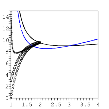
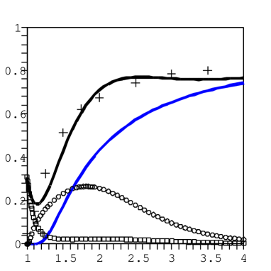
FIG. 8.: (a) The lines show twice the effective masses for quarks and gluons versus temperature $T/T_{c}$. Note that for $T<3T_{c}$ $M_{q}>M_{g}$. Circles and squares indicate estimated masses of the pion-like and rho-like $\bar{q}q$ bound states, while the crosses stand for all colored states. (b) Pressure (in units of that for a gas of massless and noninteracting quasiparticles) versus the temperature $T/T_{c}$. The crosses correspond to the $N_{f}=2$ lattice results, from Fig.2. The lower solid curve is the contribution of unbound quasiparticles, the upper includes also that of all bound states. Squares are for the pion-like and rho-like $\bar{q}q$ bound states combined, and circles for all the colored bound states.

As $\kappa_{0}$ goes through zero and changes sign, the scattering length $f(k=0)=-1/\kappa_{0}$ jump from $-\infty$ to $\infty$. As one can see from these expressions, a bound level close to zero generates significant repulsive interaction of the quasiparticles (with positive energies). As we will see shortly, an account for such repulsion reduces the contribution of the bound state to the partition function.

Let us follow the well known Beth-Uhlenbeck expression for non-ideal gases (see e.g. Landau-Lifshitz, Statistical mechanics, section 77)

$$Z_{int}= \sum_{n}e^{-|\epsilon_{n}|/T}$$ (81)

$$+{1\over\pi}\sum_{l}(2l+1)\int_{0}^{\infty}{d\delta_{l}(k)\over dk}e^{-k^{2}/mT}dk$$

where the first sum runs over all bound states with binding energies $\epsilon_{n}$ and the second over the scattering states. As the simplest example, let us consider the zero binding point $\kappa_{0}=0$, for which the expression for the scattering phase can be simplified to

$${\rm exp}(2i\delta_{0}(k))={r_{0}k/2+i\over r_{0}k/2-i}$$ (82)

and assuming that the temperature $T$ is high enough to ignore the Boltzmann factor in the integral one gets

$$Z_{int}\approx 1+{1\over\pi}(\delta_{0}(\infty)-\delta_{0}(0))=1/2\,\,.$$ (83)

Thus, at the zero binding point the repulsion reduces the contribution of the bound states to a half its value. As the virtual level moves away from zero, the contribution decreases further.

We will use a simple Fermi-like function to enforce this disappearance of the level from the statistical sum, multiplying the level contribution by an additional “reduction factor”

$$R(T)={1\over 1+{\rm exp}[C(T-T_{z.b.})]}$$ (84)

which reduces the contribution at the zero binding point $T_{z.b.}$ by 1/2 and eliminates it at higher $T$. We will use a parameter $C=2/T_{c}$.

Taking it all together, one finally gets the pressure shown in Fig. 8b. One can see that the pions and rhos peak at $T_{c}$, but become unimportant for higher $T$. The colored states are too heavy near $T_{c}$, but then their contribution to the pressure becomes comparable to that of the quasiparticle gas. There are hundreds of them, bringing quite a large statistical weight, which is however tamed by a large mass and consequently small Boltzmann factors. As a result, the total contribution follows reasonably well the lattice data points.

VIII Conclusions and discussion

In this paper we have addressed a number of issues related with the bound states in the QGP phase at not too high temperature. We have catalogued all attractive binary channels, with proper color factors and multiplicities, see Table 1. We have also presented a unified framework for analysing two body relativistic bound states of arbitrary spin and mass using first quantization arguments.

As already mentioned in the Abstract, our main task was to check the internal consistency of four (previously disconnected) lattice results: i. spectral densities from MEM analysis of the correlators; ii. static quark free energies $F(R)$; iii. quasiparticle masses; iv. bulk thermodynamics $p(T)$. We conclude that everything indeed fits well together, provided the role of multiple (colored) bound states is recognised and included.

We have parameterized recent lattice data on free energies for static quarks, calculated the corresponding effective potentials and solved the Klein-Gordon equation for charmonium, light quarks and singlet gg cases. We have found that the bound states exists at $T$ below some calculated zero-binding points. Our reported range of temperatures for charmonium and light mesons above $T_{c}$ agree rather well with what was seen from lattice correlators using the MEM [15].

Our studies of relativistic effects have found that the systems in question are not yet very relativistic, so that the relativistic corrections to the potentials do not exceed 10%. They have minor effect on binding, but are more important for the wave function at the origin. Like the authors in [22] we concluded that some non-perturbative interactions for light quarks, completely absent for static ones, should exist in order to bring the pion and sigma mass to zero at $T=T_{c}$. It is believed to be due to instanton-antiinstanton molecules, and is quasi-local: thus one can treat this interaction like a delta-function potential, using the wave function at the origin calculated without it.

Finally, we have assessed the contribution of all these bound states to the bulk pressure of the system. We have shown that as the bound state inches towards its endpoint, its contribution to the pressure becomes partially compensated by a repulsive effective interaction between the unbound quasiparticles. The contribution of the virtual level above zero quickly disappears. All in all, we have found that the summed contributions from the large number of colored bound/free states above $T_{c}$ agree well with the bulk lattice pressure.

Acknowledgments.

This work was supported in parts by the US-DOE grant DE-FG-88ER40388. We thank G. Brown and F. Karsch for many useful discussions, and also S. Fortunato, O. Kaczmarek and F. Zantow who supplied us with the electronic versions of their unpublished talks, with useful details on the static lattice potentials.

Appendix:
The Klein-Gordon equation for a Coulomb plus quasi-local potential

In this appendix we will use notations for a single body KG equation, in schematic notations $(E-V)^{2}-\vec{p}^{2}=M^{2}$, for a particle of mass $M$ in a potential $V$, chosen to be a superposition of a screened Coulomb and an additional local term

$$V=-{\alpha\over(r+0.001/M)}\,{\rm exp}(-M_{D}r)-\tilde{U}\tilde{\delta}(r)$$ (85)

where the $\tilde{\delta}(r)$ is the “nonlocal delta function”. For reasons related with instantons we will use it in the form

$$\tilde{U}\tilde{\delta}(r)=U{1\over(r^{2}+\rho^{2})^{3}}$$ (86)

with the size parameter $\rho$ to be chosen below to be $\rho=1/(0.6M)$. Note that we have chosen to ignore the coupling constant running, and regulate the Coulomb singularity.

Together with the quasiparticle mass(es) $M$ we thus already have four parameters $\alpha,M_{D},U,M$. The relevant ones are the 3 dimensionless combinations $\alpha,M_{D}/M,U/M^{2}$. To get familiar with this problem, we first studied the geometry of the fixed energy surfaces, $E=const$, in the parameter space. A section of those surfaces with two coordinate planes is shown in Fig. 7.

In Fig.(a) one can see that the (regularized) Coulomb and the instanton-induced potential are kind of complementary to each other, except near the origin: Coulomb always have levels why the quasi-local potential does not for $\tilde{U}<\tilde{U}_{min}\approx 20$. On another plane, as $M_{D}$ grows and screen the Coulomb field, one needs stronger coupling to keep the same binding.

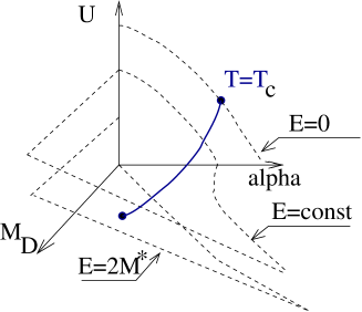
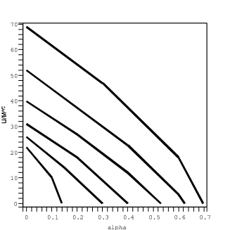
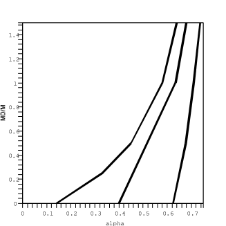
FIG. 9.: A schematic plot explaining the geometry of the surfaces of fixed binding in the 3-dimensional parameter space. Its projection on the $\alpha,U/M^{2}$ plane and on the $\alpha,M_{D}/M$ plane are shown in two subsequent plots. In the former case the values of the energy (in units of the mass) is $E/M=0,0.5,0.75,0.9,0.96,0.99$, from top to bottom. In the latter case only the lines corresponding to $E/M=0.5,0.9,0.99$ are shown (right to left).

The very left line, corresponding to $E/M=0.99$ or only 1% binding, is close to the “zero binding line” (except that it reaches the origin $\alpha=0,M_{D}=0$), to the left of which the potential in question has no bound states at all.

We have not plotted the third projection, as for $\alpha=0$ the value of $M_{D}$ is irrelevant and all lines depend on the $U$ value only. The zero binding line, separating the unbound states from the bound ones, starts at the value of $\tilde{U}_{min}\approx 20$ already mentioned. Combining 3 projections for the same binding, one can now well imagine the location and the shape of all constant energy surfaces.

REFERENCES

- [1] E. V. Shuryak, Phys. Lett. B78 (1978) 150, Yadernaya Fizika 28 (1978) 796, Phys.Rep. 61 (1980) 71.
- [2] A. M. Polyakov, Phys.Lett. B82 (1979) 2410; A. Linde, Phys. Lett. 96 (1980) 289. C. Detar, Phys. Rev. D32 (1985) 276; V. Koch, E. V. Shuryak, G. E. Brown and A. D. Jackson, Phys. Rev. D46 (1992) 3169, [Erratum-ibid. D47 (1993) 2157] T.H. Hansson and I. Zahed, Nucl. Phys. B374 (1992) 277; T.H. Hansson, M. Sporre and I. Zahed, Nucl. Phys. B427 (1994) 447; T.H. Hansson, J. Wirstam and I. Zahed, Phys. Rev. D58 (1998) 065012;
- [3] E. V. Shuryak and I. Zahed, hep-ph/0307267, submitted to PRL.
- [4] D. Teaney, J. Lauret and E.V. Shuryak, Phys. Rev. Lett. 86 (2001) 4783, more details in nucl-th/0110037. P.F. Kolb, P.Huovinen, U. Heinz, H. Heiselberg, Phys. Lett. B500 (2001) 232. More details in P. F. Kolb and U. Heinz, nucl-th/0305084.
- [5] D. Molnar and M. Gyulassy, Nucl. Phys. A697 (2002) 495; [Erratum-ibid. A703 (2002) 893]
- [6] D. Teaney nucl-th/0301099
- [7] J.Cubizolles et al., cond-mat/0308018; K.Strecker et al., cond-mat/0308318
- [8] M.W. Zwierlein et al., cond-mat/0311617.
- [9] J.M. Maldacena, Adv. Theor. Math. Phys. 2 (1998) 231, hep-th/9711200.
- [10] G.T. Horowitz and A. Strominger, Nucl. Phys. B360 (1991) 197. S.S. Gubser, I.R. Klebanov and A.A. Tseytlin, Nucl. Phys. B534 (1998) 202.
- [11] K.M. O’Hara et al, Science 298 (2002) 2179; T. Bourdel et al, Phys. Rev. Lett. 91 (2003) 020402.
- [12] G. Policastro, D. T. Son and A. O. Starinets, Phys. Rev. Lett. 87 (2001) 081601.
- [13] T. Matsui and H. Satz, Phys. Lett. B178 (1986) 416.
- [14] F. Karsch, M. T. Mehr and H. Satz, Z. Phys. C37 (1988) 617.
- [15] S. Datta, F. Karsch, P. Petreczky and I. Wetzorke, hep-lat/0208012; M. Asakawa and T. Hatsuda, Nucl. Phys. A715 (2003) 863c; hep-lat/0308034
- [16] F. Karsch et al Nucl. Phys. B715 (2003) 701.
- [17] P. Petreczky, F. Karsch, E. Laermann, S. Stickan, I. Wetzorke, Nucl. Phys. Proc. Suppl. 106 (2002) 513.
- [18] F. Karsch, AIP Conf. Proc. 631 (2003) 112.
- [19] E.V. Shuryak and I. Zahed, Phys. Rev. D69 (2004) 014011.
- [20] E.V. Shuryak, Zh.E.T.F 74 (1978) 408, (Sov. Phys. JETP 47 (1978) 212),
- [21] C.G. Darwin, Proc. Roy. Soc. Lond. Ser. A118 (1928) 654, W. Gordon, Z. Physik 48 (1928) 11.
- [22] G. E. Brown, C. H. Lee, M. Rho and E. Shuryak, hep-ph/0312175.
- [23] A. R. Edmonds, “Angular Momentum in Quantum Mechanics”, Ed. Princeton (1974), pp 83-85.
- [24] S. Wolfram, http://mathworld.wolfram.com/CubicEquation.html.
- [25] V. Hund and H. Pilkuhn, J. Phys. B33 (2000) 1617
- [26] A. Kihlberg, R. Cornelius and M. Mukunda, Phys. Rev. D23 (1981) 2201.
- [27] E. V. Shuryak, Nucl. Phys. A717 (2003) 291.
- [28] O. Kaczmarek, S. Ejiri, F. Karsch, E. Laermann and F. Zantow, hep-lat/0312015.
- [29] T. Schafer and E. V. Shuryak, Rev. Mod. Phys. 70 (1998) 323
- [30] A. Peshier, B. Kampfer, O. P. Pavlenko and G. Soff, Phys. Rev. D54 (1996) 2399.
- [31] P. Levai and U. W. Heinz, Phys. Rev. C57 (1998) 1879.
- [32] S.J. Rey, S. Theisen and J.T. Yee, Nucl. Phys. B527 (1998) 171.