2INFN, Sezione di Genova, Via Dodecaneso 33, 16146 Genova, Italy
3NIKHEF Theory Group, Kruislaan 409, 1098 SJ Amsterdam, The Netherlands
4CERN, CH–1211 Geneva 23, Switzerland
5Department of Physics and Astronomy, Michigan State University, East Lansing, MI 48824-1116, USA
6Cavendish Laboratory, University of Cambridge, Madingley Road, Cambridge CB3 0HE, UK
7DAMTP, Centre for Mathematical Science, Wilberforce Road, CB3 0WA, Cambridge, UK
8HEP Division, Argonne National Laboratory, 9700 Cass Ave., Argonne IL 60439, USA
9 Southern Methodist University, Department of Physics, Dallas, TX 75275-0175, USA
10Institut für Theoretische Physik, RWTH Aachen, 52056 Aachen, Germany
11Institut für Theoretische Physik und Astrophysik, Universität Würzburg, D-97074 Würzburg, Germany
12DESY-Theorie, 22603 Hamburg, Germany
13 Department of Physics and Astronomy, University of Sheffield, UK
14Max Planck Institute für Physik, 80805 München, Germany
15 Department of Physics, University of Florida, Gainesville, Florida, 32611, USA
16INFN, Sezione di Torino, Via P. Giuria 1, I-10125 Torino, Italy
17New Mexico Center for Particle Physics, University of New Mexico, USA
18 Dipartimento di Fisica ”Galileo Galilei”, Universit\a‘a di Padova, Italy
19Moscow State University, Moscow, Russia
20LAPTH, F-79941 Annecy-le-Vieux, France
21II Institut für Theoretische Physik,Universität Hamburg, Luruper Chaussee 149, D-22761 Hamburg, Germany
22Institut fur Theoretische Teilchenphysik, Universität Karlsruhe, Germany
23Helsinki Institute of Physics, P.O. Box 64, Helsinki, Finland
24Dipartimento di Fisica Teorica, Università di Torino, Via P. Giuria 1, I-10125 Torino, Italy
25Centro Studi e Ricerche “Enrico Fermi”, via Panisperna, 89/A - 00184 Rome, Italy
26School of Physics and Astronomy, University of Southampton, Highfield, Southampton SO17 1BJ, UK
27Fermi National Accelerator Laboratory, Batavia, IL 60510-500, USA
28Institute of Theoretical Science, 5203 University of Oregon, Eugene, OR 97403-5203, USA
29FESB, University of Split, Split, Croatia
30LPTHE, Universities of Paris VI and VII and CNRS UMR 7589, Paris, France
31Department of Physics, Shandong University, Jinan, Shandong 250100, China
32Department of Theoretical Physics, Lund University, S-223 62 Lund, Sweden
33University of Debrecen and Institute of Nuclear Research of the Hungarian Academy of Sciences, H-4001 Debrecen, PO Box 51, Hungary
THE QCD/SM WORKING GROUP:
Summary Report
Abstract
Recently the collider physics community has seen significant advances in the formalisms and implementations of event generators. This review is a primer of the methods commonly used for the simulation of high energy physics events at particle colliders. We provide brief descriptions, references, and links to the specific computer codes which implement the methods. The aim is to provide an overview of the available tools, allowing the reader to ascertain which tool is best for a particular application, but also making clear the limitations of each tool.
Due to its long length and stand-alone nature, the Monte Carlo Guidebook entry in the Les Houches proceedings has been published as a separate document (hep-ph/0403045). The table of contents follows.
Report of the Working Group on Quantum Chromodynamics and the Standard Model for the Workshop “Physics at TeV Colliders”, Les Houches, France, 26 May - 6 June, 2003.
1 FOREWORD 111M. Dobbs’ work was supported in part by the Director, Office of Science, Office of Basic Energy Sciences, of the U.S. Department of Energy under Contract No. DE-AC03-76SF00098.
Among the many physics processes at TeV hadron colliders, we look most eagerly for those that display signs of the Higgs boson or of new physics. We do so however amid an abundance of processes that proceed via Standard Model (SM) and in particular Quantum Chromodynamics (QCD) interactions, and that are interesting in their own right. Good knowledge of these processes is required to help us distinguish the new from the known. Their theoretical and experimental study teaches us at the same time more about QCD/SM dynamics, and thereby enables us to further improve such distinctions. This is important because it is becoming increasingly clear that the success of finding and exploring Higgs boson physics or other New Physics at the Tevatron and LHC will depend significantly on precise understanding of QCD/SM effects for many observables.
To improve predictions and deepen the study of QCD/SM signals and backgrounds was therefore the ambition for our QCD/SM working group at this Les Houches workshop. Members of the working group made significant progress towards this on a number of fronts. A variety of tools were further developed, from methods to perform higher order perturbative calculations or various types of resummation, to improvements in the modelling of underlying events and parton showers. Furthermore, various precise studies of important specific processes were conducted.
A signficant part of the activities in Les Houches revolved around Monte Carlo simulation of collision events. A number of contributions in this report reflect the progress made in this area. At present a large number of Monte Carlo programs exist, each written with a different purpose and employing different techniques. Discussions in Les Houches revealed the need for an accessible primer on Monte Carlo programs, featuring a listing of various codes, each with a short description, but also providing a low-level explanation of the underlying methods. This primer has now been compiled and a synopsis of it is included here as the first contribution to this report (see below for where to obtain the full document).
This report reflects the hard and creative work by the many contributors which took place in the working group. After the MC guide description, the next contributions report on progress in describing multiple interactions, important for the LHC, and underlying events. An announcement of a Monte Carlo database, under construction, is followed by a number of contributions improving parton shower descriptions. Subsequently, a large number of contributions address resummations in various forms, after which follow studies of QCD effects in pion pair, top quark pair and photon pair plus jet production. After a study of electroweak corrections to hadronic precision observables, the report ends by presenting recent progress in methods to compute finite order corrections at one-loop with many legs, and at two-loop.
2 LES HOUCHES GUIDEBOOK TO MONTE CARLO GENERATORS FOR HADRON COLLIDER PHYSICS
Editors: M. Dobbs, S. Frixione, E. Laenen, K. Tollefson
Contributing Authors:
H. Baer,
E. Boos,
B. Cox,
M. Dobbs,
R. Engel,
S. Frixione,
W. Giele,
J. Huston,
S. Ilyin,
B. Kersevan,
F. Krauss,
Y. Kurihara,
E. Laenen,
L. Lönnblad,
F. Maltoni,
M. Mangano,
S. Odaka,
P. Richardson,
A. Ryd,
T. Sjöstrand,
P. Skands,
Z. Was,
B.R. Webber,
D. Zeppenfeld
3 MULTIPLE INTERACTIONS AND BEAM REMNANTS 222Contributed by: T. Sjöstrand and P. Skands
3.1 Introduction
Hadrons are composite systems of quarks and gluons. A direct consequence is the possibility to have hadron–hadron collisions in which several distinct pairs of partons collide with each other, i.e. multiple interactions, a.k.a. multiple scatterings. At first glance, the divergence of the perturbative -channel one-gluon-exchange graphs in the limit implies an infinity of interactions per event. However, the perturbative framework does not take into account screening from the fact that a hadron is in an overall colour singlet state. Therefore an effective cutoff of the order of one to a few GeV is introduced, representing an inverse colour correlation distance inside the hadron. For realistic values most inelastic events in high-energy hadronic collisions should then contain several perturbatively calculable interactions, in addition to whatever nonperturbative phenomena may be present.
Although most of this activity is not hard enough to play a significant role in the description of high– jet physics, it can be responsible for a large fraction of the total multiplicity (and large fluctuations in it) for semi-hard (mini-)jets in the event, for the details of jet profiles and for the jet pedestal effect, leading to random as well as systematic shifts in the jet energy scale. Thus, a good understanding of multiple interactions would seem prerequisite to carrying out precision studies involving jets and/or the underlying event in hadronic collisions.
In an earlier study [1], it was argued that all
the underlying event activity is triggered by the multiple interactions
mechanism. However, while the origin of underlying events is thus
assumed to be perturbative, many nonperturbative aspects still need to be
considered and understood:
(i) What is the detailed mechanism and functional form of the
dampening of the perturbative cross section at small ?
(Certainly a smooth dampening is more realistic than a sharp
cutoff.)
(ii) Which energy dependence would this mechanism have?
(iii) How is the internal structure of the proton reflected in an
impact-parameter-dependent multiple interactions rate, as manifested
e.g. in jet pedestal effects?
(iv) How can the set of colliding partons from a hadron be
described in terms of correlated multiparton distribution functions
of flavours and longitudinal momenta?
(v) How does a set of initial partons at some low perturbative
cutoff scale, ‘initiators’, evolve into such a set of colliding partons?
(Two colliding partons could well have a common initiator.)
Is standard DGLAP evolution sufficient, or must BFKL/CCFM effects be
taken into account?
(vi) How would the set of initiators correlate with the flavour
content of, and the longitudinal momentum sharing inside, the left-behind
beam remnant?
(vii) How are the initiator and remnant partons correlated by
confinement effects (‘primordial ’)?
(viii) How are all produced partons, both the
interacting and the beam-remnant ones,
correlated in colour? Is the large number-of-colours limit
relevant, wherein partons can be hooked up into strings (with quarks as
endpoints and gluons as intermediate kinks) representing a linear
confinement force [2]?
(ix) How is the original baryon number of an incoming proton
reflected in the colour topology?
(x) To what extent would a framework with independently
fragmenting string systems, as defined from the colour topology, be
modified by the space–time overlap of several strings?
Needless to say, we should not expect to find a perfect solution to any of these issues, but only successively improved approximations. The framework in [1] is very primitive in a number of respects. Nevertheless, it has turned out to be quite successful. Thus the Pythia Tune A of R.D. Field [3] is capable of describing a host of jet and minimum-bias event data at the Tevatron. The model appears inadequate to fully describe correlations and fluctuations, however, and we would expect a poor performance for several topics not yet studied experimentally.
In particular, only very simple beam remnant structures could technically be dealt with in [1]. One recent development was the extension of the standard Lund string framework [2] to include a junction fragmentation description [4] that allows the hadronization of nontrivial colour topologies containing non-zero baryon number. In the context of multiple interactions, this improvement means that almost arbitrarily complicated baryon beam remnants may now be dealt with, hence many of the restrictions present in the old model are no longer necessary.
Here, we report on the development of a new model for the flavour-, colour-, and momentum-correlated partonic structure involved in a hadron–hadron collision, i.e. partly addressing several of the points above. We first present the main work on flavour and momentum space correlations, and thereafter separately the very thorny issue of colour correlations, before concluding. A more complete description of the model, also including references to experimental data and other theoretical ideas, and with comments on all the issues, may be found in [5]. A toy model study of the first two points is found in [6]. The Pythia manual [7] contains some complementary information.
3.2 Correlated Parton Densities
Consider a hadron undergoing multiple interactions in a collision. Such an object should be described by multi-parton densities, giving the joint probability of simultaneously finding partons with flavours , carrying momentum fractions inside the hadron, when probed by interactions at scales . However, we are nowhere near having sufficient experimental information to pin down such distributions. Therefore, and wishing to make maximal use of the information that we do have, namely the standard one-parton-inclusive parton densities, we propose the following strategy.
As described in [1], the interactions may be generated in an ordered sequence of falling . For the hardest interaction, all smaller scales may be effectively integrated out of the (unknown) fully correlated distributions, leaving an object described by the standard one-parton distributions, by definition. For the second and subsequent interactions, again all lower– scales can be integrated out, but the correlations with the first cannot, and so on. Thus, we introduce modified parton densities, that correlate the ’th interaction and its shower evolution to what happened in the previous ones.
The first and most trivial observation is that each interaction removes a momentum fraction from the hadron remnant. Already in [1] this momentum loss was taken into account by assuming a simple scaling ansatz for the parton distributions, , where is the momentum remaining in the beam hadron after the first interactions. Effectively, the PDF’s are simply ‘squeezed’ into the range .
Next, for a given baryon, the valence distribution of flavour after interactions, , should integrate to the number of valence quarks of flavour remaining in the hadron remnant. This rule may be enforced by scaling the original distribution down, by the ratio of remaining to original valence quarks , in addition to the scaling mentioned above.
Also, when a sea quark is knocked out of a hadron, it must leave behind a corresponding antisea parton in the beam remnant. We call this a companion quark. In the perturbative approximation the sea quark and its companion come from a gluon branching (it is implicit that if is a quark, is its antiquark). Starting from this perturbative ansatz, and neglecting other interactions and any subsequent perturbative evolution of the , we obtain the distribution from the probability that a sea quark , carrying a momentum fraction , is produced by the branching of a gluon with momentum fraction , so that the companion has a momentum fraction ,
| (1) |
with the usual DGLAP gluon splitting kernel. A simple ansatz is here used for the gluon. Normalizations are fixed so that a sea quark has exactly one companion. Qualitatively, is peaked around , by virtue of the symmetric splitting kernel.
Without any further change, the reduction of the valence distributions and the introduction of companion distributions, in the manner described above, would result in a violation of the total momentum sum rule, that the -weighted parton densities should integrate to : by removing a valence quark from the parton distributions we also remove a total amount of momentum corresponding to , the average momentum fraction carried by a valence quark of flavour ,
| (2) |
and by adding a companion distribution we add an analogously defined momentum fraction.
To ensure that the momentum sum rule is still respected, we assume that the sea+gluon normalizations fluctuate up when a valence distribution is reduced and down when a companion distribution is added, by a multiplicative factor
| (3) |
The requirement of a physical range is of course still maintained by ‘squeezing’ all distributions into the interval . The full parton distributions after interactions thus take the forms
| (4) | |||||
| (5) |
where () denotes the original valence (sea) distribution of flavour , and the index on the companion distributions counts different companion quarks of the same flavour .
After the perturbative interactions have each taken their fraction of longitudinal momentum, the remaining momentum is to be shared between the beam remnant partons. Here, valence quarks receive an picked at random according to a small- valence-like parton density, while sea quarks must be companions of one of the initiator quarks, and hence should have an picked according to the distribution introduced above. In the rare case that no valence quarks remain and no sea quarks need be added for flavour conservation, the beam remnant is represented by a gluon, carrying all of the beam remnant longitudinal momentum.
Further aspects of the model include the possible formation of composite objects in the beam remnants (e.g. diquarks) and the addition of non-zero primordial values to the parton shower initiators. Especially the latter introduces some complications, to obtain consistent kinematics. Details on these aspects are presented in [5].
3.3 Colour Correlations
The initial state of a baryon may be represented by three valence quarks, connected antisymmetrically in colour via a central junction, which acts as a switchyard for the colour flow and carries the net baryon number, Fig. 1a.
The colour-space evolution of this state into the initiator and remnant partons actually found in a given event is not predicted by perturbation theory, but is crucial in determining how the system hadronizes; in the Lund string model [2], two colour-connected final state partons together define a string piece, which hadronizes by successive non-perturbative breakups along the string. Thus, the colour flow of an event determines the topology of the hadronizing strings, and consequently where and how many hadrons will be produced. The question can essentially be reduced to one of choosing a fictitious sequence of gluon emissions off the initial valence topology, since sea quarks together with their companion partners are associated with parent gluons, by construction.
The simplest solution is to assume that gluons are attached to the initial quark lines in a random order, see Fig. 1b. If so, the junction would rarely be colour-connected directly to two valence quarks in the beam remnant, and the initial-state baryon number would be able to migrate to large and small values. While such a mechanism should be present, there are reasons to believe that a purely random attachment exaggerates the migration effects. Hence a free parameter is introduced to suppress gluon attachments onto colour lines that lie entirely within the remnant, so that topologies such as Fig. 1c become more likely.
This still does not determine the order in which gluons are attached to the colour line between a valence quark and the junction. We consider a few different possibilities: 1) random, 2) gluons are ordered according to the rapidity of the hard scattering subsystem they are associated with, and 3) gluons are ordered so as to give rise to the smallest possible total string lengths in the final state. The two latter possibilities correspond to a tendency of nature to minimize the total potential energy of the system, i.e. the string length. Empirically such a tendency among the strings formed by multiple interactions is supported e.g. by the observed rapid increase of with . It appears, however, that a string minimization in the initial state is not enough, and that also the colours inside the initial-state cascades and hard interactions may be nontrivially correlated. These studies are still ongoing, and represent the major open issues in the new model.
3.4 Conclusion
A new model for the underlying event in hadron–hadron collisions [5] has been introduced. This model extends the multiple interactions mechanism proposed in [1] with the possibility of non-trivial flavour and momentum correlations, with initial- and final-state showers for all interactions, and with several options for colour correlations between initiator and remnant partons. Many of these improvements rely on the development of junction fragmentation in [4].
This is not the end of the line. Rather we see that many issues remain to understand better, such as colour correlations between partons in interactions and beam remnants, whereas others have not yet been studied seriously, such as the extent to which two interacting partons stem from the same initiator. Theoretical advances alone cannot solve all problems; guidance will have to come from experimental information. The increased interest in such studies bodes well for the future.
4 DESCRIBING MINIMUM BIAS AND THE UNDERLYING EVENT AT THE LHC IN PYTHIA AND PHOJET 333Contributed by: A. Moraes, C. Buttar, and I. Dawson
4.1 Introduction
Our ability to describe parton scatterings through QCD depends on the amount of transverse momenta with respect to the collision axis (pt) involved in a given scattering [8]. QCD has been fairly successful in describing quark, anti-quark and gluon scatterings involving large amounts of transverse momenta (p), also known as “hard” interactions. On the other hand, QCD simply cannot be applied to interactions with small transverse momenta (or “soft” interactions) because the strong coupling constant, , becomes too large for perturbation theory to be applied and QCD models suffer from divergent cross sections as [8]. Most high-energy hadron collisions are dominated by soft partonic interactions.
A full picture of high-energy hadron collisions will typically combine perturbative QCD to explain parton interactions where it is applicable (high-pt scatterings), with an alternative phenomenological approach to describe soft processes. Examples of these are the Dual Parton Model (DPM) [9] and modified versions of QCD in which the divergencies presented by the running coupling constant are phenomenologically corrected to reproduce experimental observations [1].
In this article we investigate two Monte Carlo (MC) event generators, PYTHIA6.214 [10, 11] and PHOJET1.12 [12, 13], focusing on their models for soft interactions in hadron-hadron collisions. Aiming to check the consistency of these models, we compare their predictions to wide range of data for minimum bias and the underlying event. A tuning for PYTHIA6.214 is presented and examples of its predictions are compared to those generated with PHOJET1.12 . Predictions for levels of particle production and event activity at the LHC for interactions dominated by soft processes such as minimum bias interactions and the underlying event associated to jet production are also discussed.
4.2 PYTHIA Model for Hadron Collisions
A comprehensive description of PYTHIA can be found at [11] and references therein. The evolution of a hadronic event generated by PYTHIA is based on parton-parton scatterings [10, 11]. In this model the total rate of parton interactions, , as a function of the transverse momentum scale pt, is assumed to be given by perturbative QCD. At reasonably large pt values (p 2 GeV) parton scatterings can be correctly described by the standard perturbative QCD, but to extend the parton-parton scattering framework to the low-pt region a regularisation to correct the divergence in the cross-section is introduced.
In order to deal with low-pt interactions, PYHTIA introduces a cut-off parameter p given by
| (6) |
which can be interpreted as the inverse of some colour screening length in the hadron [6]. There are two strategies, or scenarios, to implement the cut-off parameter defined by equation 6.
In the first one, labelled “simple” scenario, an effective cut-off is established at , which means that for . This model assumes that different pairwise interactions take place essentially independent of each other, and that therefore the number of interactions in an event is given by a Poissonian distribution [1]. In the second approach, called the ‘complex’ scenario, the probability associated with each interacting parton depends on the assumed matter distribution inside the colliding hadrons. In the ‘complex’ scenario an impact parameter dependent approach is therefore introduced [1].
The parameters defining p are PARP(81), PARP(82), PARP(89) and PARP(90). The factor 1.9 GeV is defined in the simple scenario by PARP(81) and by PARP(82) in the complex scenario. The energy scale 1 TeV is defined by PARP(89) and is included in equation (1) to be a convenient tuning parameter rather than a parameter with physical meaning. PARP(90) gives the power with which p varies with the centre of mass energy, . The default option is set as PARP(90)=0.16 [10, 11].
4.3 PHOJET
The physics model used in the MC event generator PHOJET combines the ideas of the DPM [9] with perturbative QCD [8] to give an almost complete picture of high-energy hadron collisions [12, 13, 14].
PHOJET is formulated as a two-component model containing contributions from both soft and hard interactions. The DPM is used describe the dominant soft processes and perturbative QCD is applied to generate hard interactions [13].
The model employed by PHOJET is based on the calculation of scattering amplitudes, taking into account the unitarization principle. Comparisons between the calculated results for cross-sections and the available data are used to determine the unknown model parameters (couplings, Pomeron intercepts and slope parameters), which are needed to generate multiparticle final states produced in inelastic interactions [12, 13].
The soft, , and hard, , cross sections are inclusive cross sections and the average multiplicities of soft and hard scatterings in an inelastic event are
| (7) |
respectively. The hard scatterings are mostly independent of each other, being related only by the sharing of energy and momentum of the incoming protons. These multiplicities increase with the colliding centre-of-mass energy. For pp collisions at TeV a considerable part of interactions is expected to have more than one hard or soft scattering.
4.4 Minimum Bias Interactions
Throughout this article, we will associate minimum bias events with non-single diffractive inelastic (NSD) interactions, following the experimental definition used in [15, 16, 17, 18, 19]. In the language of the MC event generators used in this work, this means that subprocesses 94 and 95 are switched on in PYTHIA6.214 (MSUB(94)=1 and MSUB(95)=1), and processes IPRON(1,1), IPRON(4,1) and IPRON(7,1) in PHOJET1.12. For both generators, we also adapt the MC distributions to the data by setting and as stable particles.
4.4.1 KNO Distribution
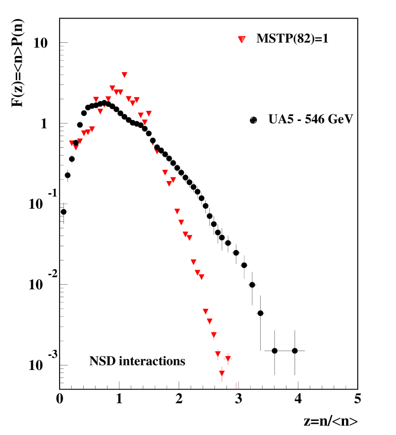
The KNO distribution [20] has been widely used as an important tool for studying multiple particle production in inelastic and NSD events. The observed KNO scaling violation for p collisions at energies higher than those achieved at ISR [15, 16] has been explained by the rising number of multiple parton scatterings as [18, 19]. KNO distributions are therefore good tools to exploit how well hadronic models can describe the event properties associated to multiple parton scattering.
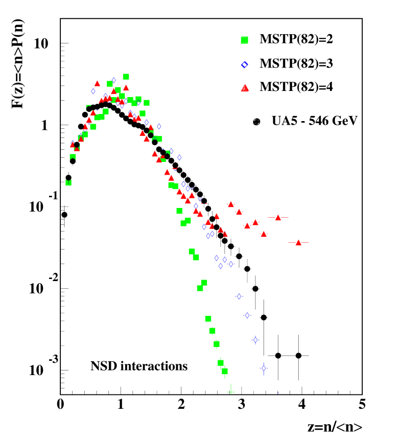
By default PYTHIA is set to use multiple parton interactions. Nevertheless, one still has to define how the divergency for scatterings with p will be treated by the event generator. PYTHIA allows two different phenomenological approaches: simple (MSTP(82)=1) and complex scenarios (MSTP(82)=2, 3 or 4). Selecting the complex scenario one has also the choice of selecting different matter distributions for the colliding hadrons: uniform (MSTP(82)=2), single Gaussian (MSTP(82)=3) and double Gaussian (MSTP(82)=4) matter distributions.
|
|
|---|---|
| (a) | (b) |
Figure 2 shows KNO distributions for NSD p collisions at = 546 GeV. We compare distributions generated by PYTHIA’s simple and complex scenarios to UA5 data [16]. Apart from the mentioned changes in the setting MSTP(82), all other parameters are set to use PYTHIA’s default options, as described in [11]. Figure 2(a) shows that using the simple scenario (MSTP(82)=1), which is the default PYTHIA6.214 option [11], the generated distributions fail to reproduce the data, especially in the region of high z (z1.5). This is the region of events with particle multiplicities several times greater than the average multiplicity. Distributions generated using the complex scenario vary with the hadronic matter distribution selected for each case, as can be seen in figure 2(b) .
The comparisons of KNO distributions shown in figure 2(b) indicate that the matter distribution used to describe the colliding hadrons does affect the probability of particle production in minimum bias events. Although in the comparisons shown in figure 2 the best agreement to the data was obtained by selecting the complex scenario with the single Gaussian matter distribution option, we shall adopt the complex scenario with a double Gaussian matter distribution (MSTP(82)=4) as our preferred choice.
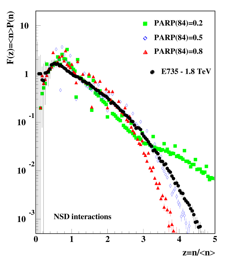
This is done because by choosing the double Gaussian option, the user is able to control some of the properties of this matter distribution. Hadrons described by this distribution have a small core region of radius a2 containing a fraction of the total hadronic matter. This core is embedded in a larger volume of radius a1 containing the remaining fraction of matter, i.e., (1 - ) of the total hadronic matter. The parameter PARP(83) controls the portion of the total hadronic matter assigned to the core of the hadron. The ratio a2/a1 is given by the parameter PARP(84). By default, PYTHIA sets PARP(83)=0.5 and PARP(84)=0.2 describing any given hadron as a body with half of its matter concentrated within a core which is limited by a radius a2 = 20% of the hadron radius a1 [11].
|
|
|---|---|
| (a) | (b) |
As shown in figure 3(a) considerable changes in the high-z tale of the KNO distributions are observed as the core radius varies from 20% to 50% and 80% of the radius of the colliding hadrons. As the core is made harder and denser (smaller core-radius) the overlap between two colliding cores makes high-pt partonic scatterings more likely, yielding higher multiplicity events more often. When two relatively softer cores (larger radius) overlap in a collision, the generated activity will be smaller and softer, hence producing high-multiplicity events less frequently.
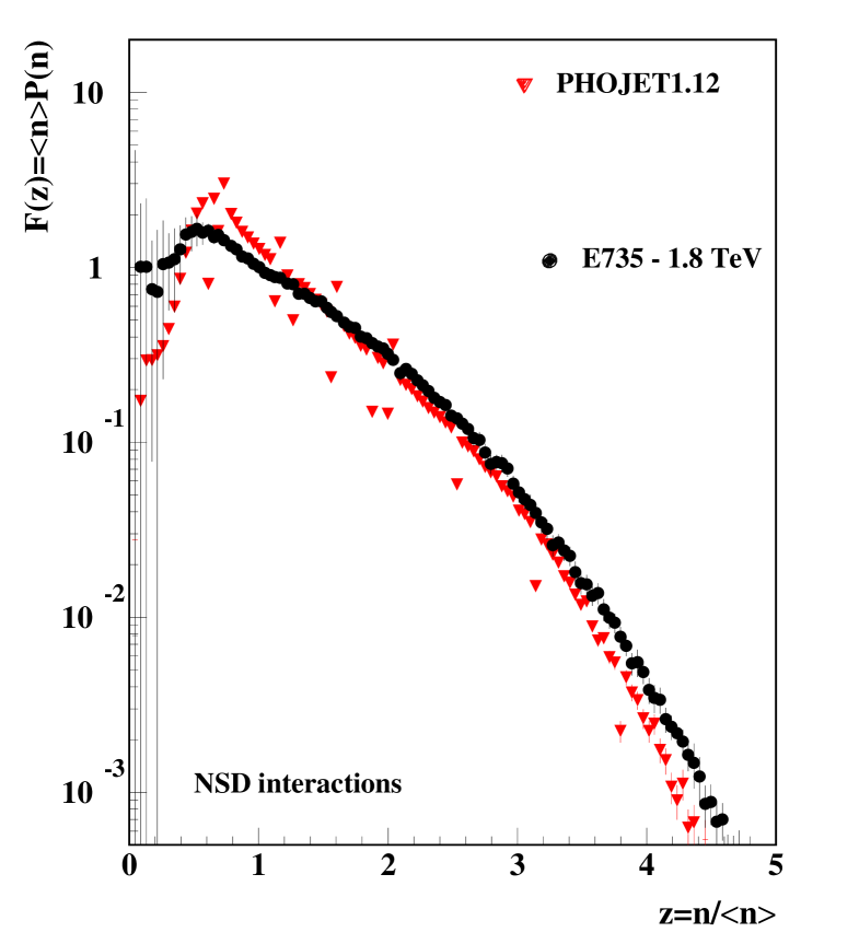
Figure 3(b) shows a comparison between PHOJET1.12 and the KNO distribution measured by E735 [18, 19] for NSD p collisions at = 1.8 TeV. Describing hadron collisions using the multiple Pomeron exchange mechanism proposed by the DPM [9, 13] and the QCD picture for high-pt interactions, PHOJET1.12 is in good agreement to the data.
4.4.2 Pseudorapidity Distribution
The rate of parton-parton scattering in a hadronic collision is strongly correlated to the observed particle multiplicity and the pseudorapidity distribution of produced particles. This happens because multiple parton interactions convert part of the collision energy that would otherwise be carried by the fast moving system of beam-remnants in the forward regions, into low-pt particles which populate the central region.
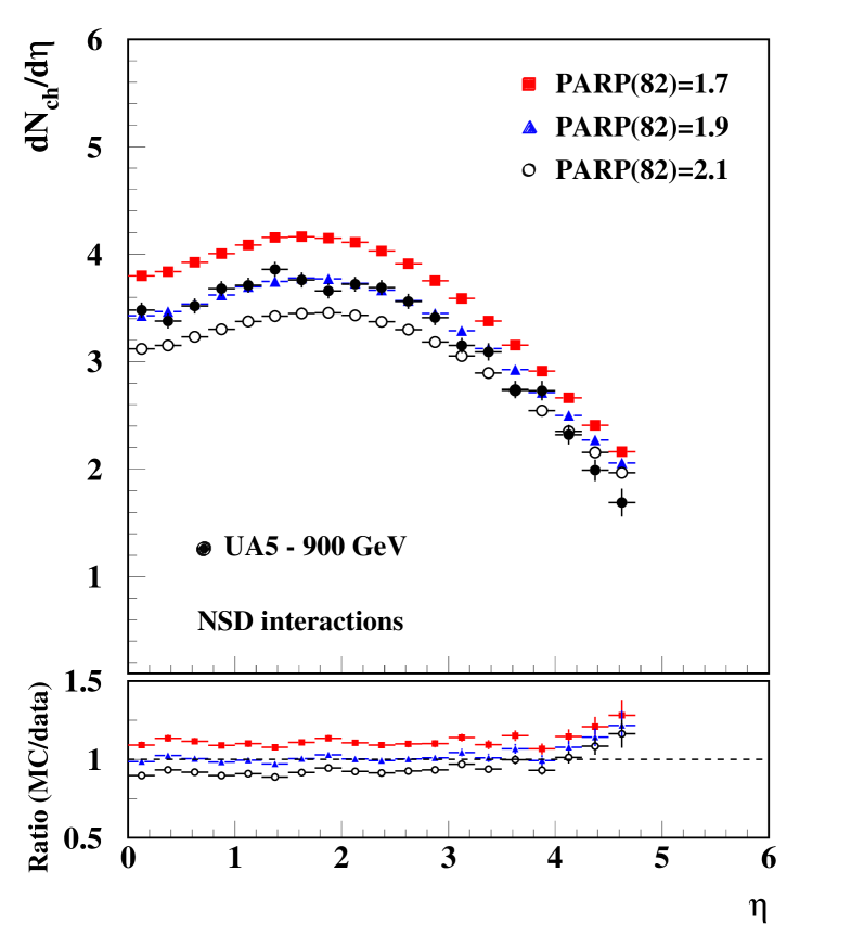
In PYTHIA, one of the main parameters used to regulate the rate of parton-parton interactions is p given by equation 6. Low values of p imply in high rates of parton-parton scatterings and hence in high levels of particle multiplicity. Increasing p the opposite is expected.
|
|
|---|---|
| (a) | (b) |
As can be seen in figure 4(a), increasing PARP(82) from 1.7 to 1.9 and 2.1, which effectively increases the p used by PYTHIA6.214, the charged particle density, dNch/d, decreases. Notice that relatively small changes in PARP(82) () can cause significant variations in the plateau of dNch/d.
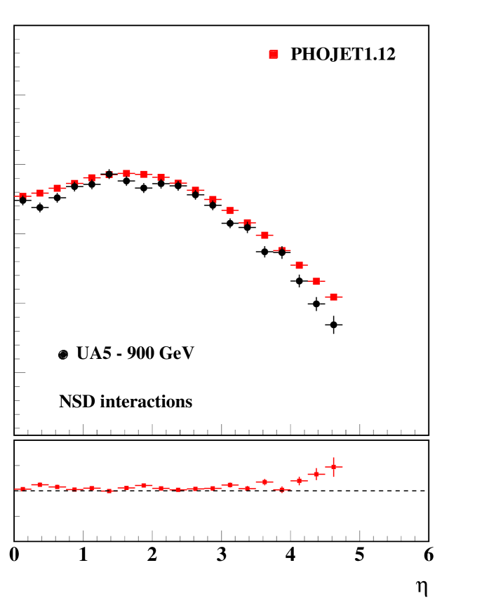
In PHOJET, multiple Pomeron exchanges predicted by the DPM control the plateau of dNch/d. Similarly to PYTHIA, this model also depends on a p which is used to connect the soft and hard components of a hadronic interaction. PHOJET1.12 has its default options tuned for p GeV. Figure 4(b) shows dNch/d generated by PHOJET1.12 with its default cuts, compared to UA5 data [21]. There is a good agreement between PHOJET1.12 predictions and the data.
4.5 The Underlying Event
In a hadronic event containing jets, the underlying event (UE) consists of all event activity except the two outgoing hard scattered jets [22]. As for minimum bias events, soft interactions and the mechanism of multiple parton interaction play an important role in the structure of the underlying event and ought to be carefully considered by any model attempting to describe the underlying event.
The conditions applied to particle selection and to the event region to be investigated are described in Ref. [22]. The region transverse to the leading jet is used to study the UE and is defined by , where the angular difference in the azimuthal angle is given by .
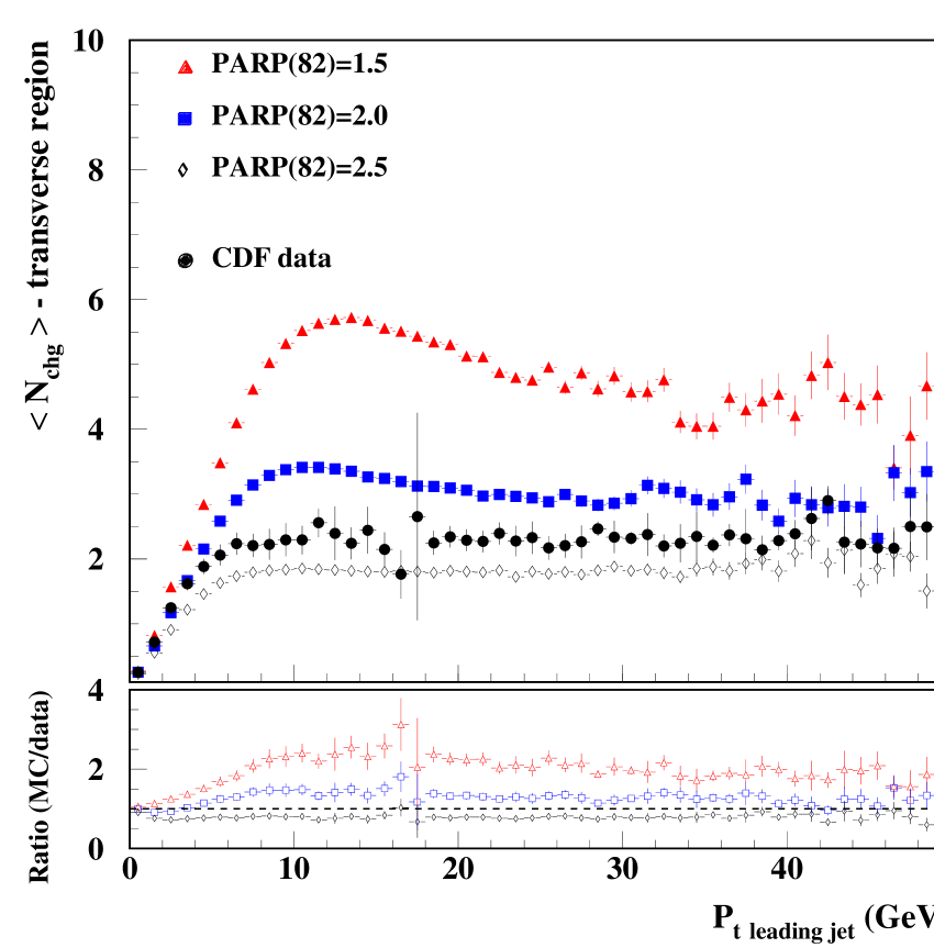
Figure 5(a) shows PYTHIA6.214 - MSTP(82)=4 distributions generated with different values of PARP(82), i.e. different p, compared to the data for the average charged particle multiplicity in the transverse region. Increasing p, which corresponds to a decrease on the rate of semi-hard parton scatterings, decreases. This effect is similar to the one observed in figure 4(a) for minimum bias charged particle density distributions dNch/d.
|
|
|---|---|
| (a) | (b) |
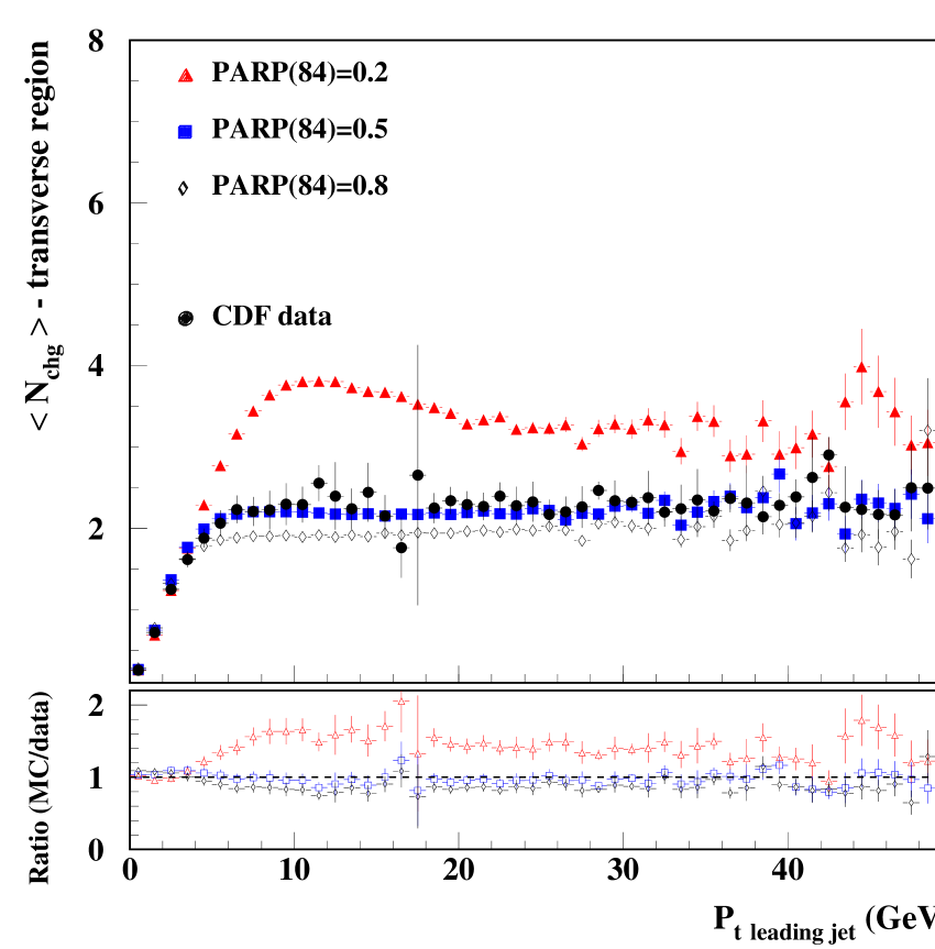
As shown in figure 5(b), depending on the core size variation (PARP(84)) the plateau level of can suffer severe changes. For example, changing PARP(84) from 0.2 to 0.5 reduces the plateau of by nearly a factor of two, while a further increase in PARP(84) from 0.5 to 0.8 only reduces the plateau by %.
Jets are likely to be produced when there is a core overlap in the hadronic collision. Smaller and dense cores imply that events with a core overlap have also a large overlap of less dense matter regions which surround the core, and when overlapped generate high rates of soft interactions causing the higher plateaus observed in the distributions shown in figure 5(b). Larger cores also imply in smaller soft surrounding regions in the colliding hadrons, hence producing lower multiplicity (and ) distributions in the UE.
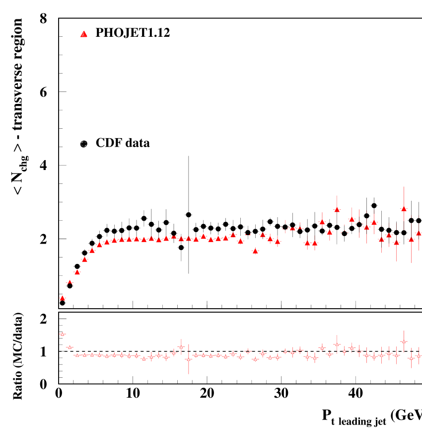
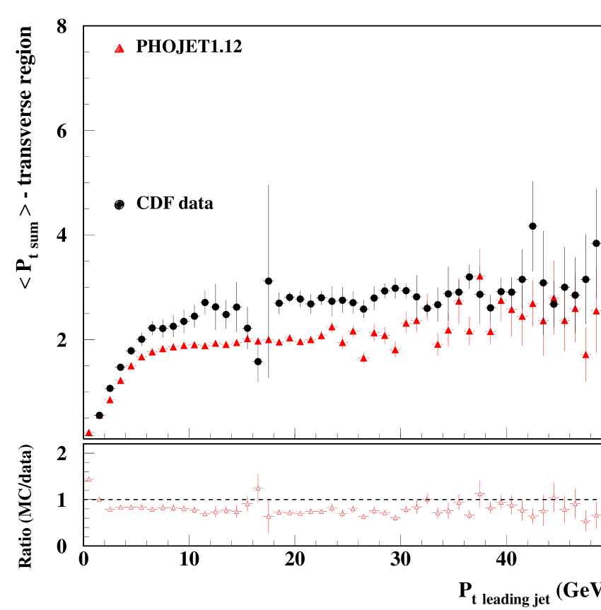
Figure 6 shows PHOJET1.12 predictions compared to data for: (a) average multiplicity in the transverse region and (b) average in the transverse region.
|
|
|---|---|
| (a) | (b) |
PHOJET1.12 reproduces reasonably well the data for the UE multiplicity distribution, as displayed in figure 6 (a). However, it underestimates the average distribution (figure 6(b) ). The measured distribution is underestimated by PHOJET1.12 by %.
4.5.1 UE vs. Minimum Bias
The CDF measurement shows that the underlying event multiplicity forms a plateau for events with P GeV at . Supposing that the transverse region in events with P GeV is uniform in azimuthal angle and in pseudorapidity , this multiplicity corresponds to 3.45 particle per unit pseudorapidity. Further corrections to detector effects and low-pt extrapolation [22] implies that there are roughly 10 charged particles per pseudorapidity unit with p GeV in the underlying event.
In p collision at 1.8 TeV, the minimum bias density, which has also been measured by CDF, gives dNch/d for [17], while the equivalent density for the underlying event is at least a factor of two larger. This comparison, though not highly accurate due to the uncertainties in estimating the particle density for the underlying event (i.e. extrapolation to low-pt and several assumptions made on the particle distribution in and ), clearly shows that the underlying event in hard scattering processes (P GeV) has much more activity than an average minimum bias event.
4.6 PYTHIA6.214 - Tuned VS. PHOJET1.12
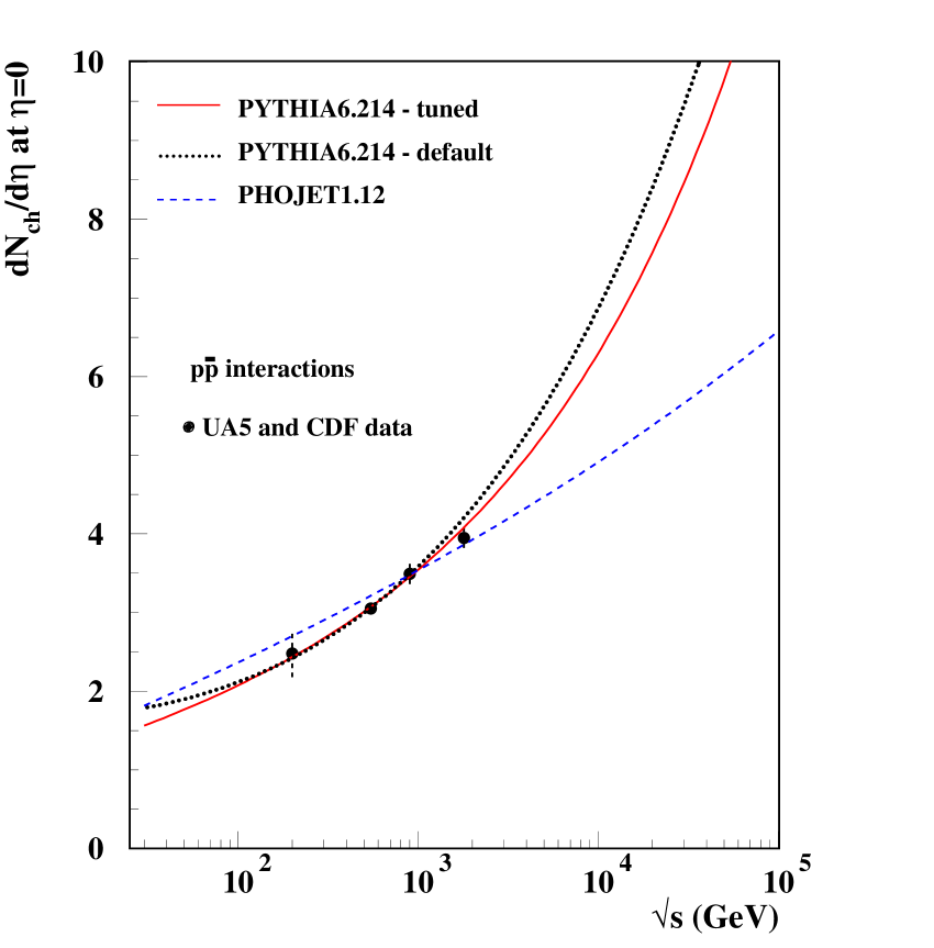
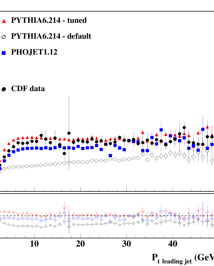
Combining the effects of variations in p and in the core-size we obtained a set of PYTHIA6.214 parameters which considerably improves PYTHIA’s description of minimum bias and underlying event distributions. Our tuned parameters for PYTHIA6.214 are displayed in table 1.
| PYTHIA6.214 - tuned | |
|---|---|
| ISUB: 11,12,13,28,53,68 | QCD partonic scattering |
| 94,95,96 | + non-diffractive + double diffractive |
| MSTP(51)=7 | CTEQ5L - selected p.d.f. |
| MSTP(81)=1 | multiple interactions |
| MSTP(82)=4 | complex scenario |
| + double Gaussian matter distribution | |
| PARP(82)=1.8 | p parameter |
| PARP(84)=0.5 | core radius: 50% of the |
| hadronic radius | |
|
|
| (a) | (b) |
|
|
| (c) | (d) |
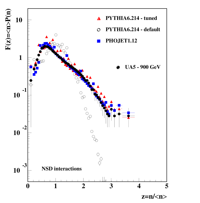
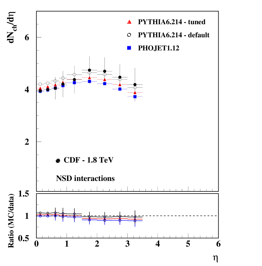
Figure 7 shows predictions generated by PYTHIA6.214 - tuned and default, and PHOJET1.12 compared to some minimum bias and underlying event distributions. The description of both minimum bias and underlying event distributions is improved by using PYTHIA6.214 - tuned compared to the predictions generated by PYTHIA’s default settings. Notice that PYTHIA6.214 - tuned and PHOJET1.12 can generate very different predictions when extrapolated to higher energies, as shown in fig. 7(c).
4.7 LHC Predictions
|
|
|---|---|
| (a) | (b) |
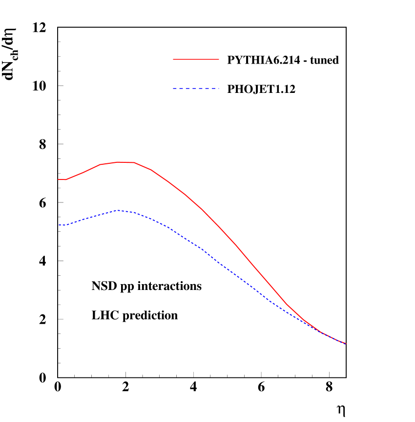
Figure 8(a) shows dNch/d distributions for minimum bias pp collisions at = 14 TeV generated by PHOJET1.12 and PYTHIA6.214 - tuned. The charged particle density generated by PHOJET1.12 and PYTHIA6.214 - tuned at is 5.13 and 6.82, respectively. In the central region () dNch/d is and , respectively for PHOJET1.12 and PYTHIA6.214 - tuned. Contrasting to the agreement shown for p collisions at = 1.8 TeV in figure 7(b), at the LHC PYTHIA6.214 - tuned generates more charged particle density in the central region than PHOJET1.12.
Compared to the charged particle density dNch/d measured by CDF at 1.8 TeV (figure 7(b) ), PYTHIA6.214 - tuned indicates a plateau rise of at the LHC in the central region while PHOJET1.12 suggests a smaller rise of .
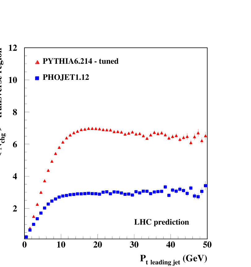
Figure 8(b) displays PYTHIA6.214 - tuned and PHOJET1.12 predictions for the average particle multiplicity in the UE for pp collisions at the LHC (charged particles with GeV and ). The distributions generated by the two models are fundamentally different. Excepting the events with P GeV, PYTHIA6.214 - tuned generates greater activity than PHOJET1.12 in the UE. The average multiplicity in the UE for P GeV reaches a plateau at charged particles according to PYTHIA6.214 - tuned and according to PHOJET1.12. Compared to the UE distributions measured by CDF at 1.8 TeV (figure 7(d) ), PYTHIA6.214 - tuned indicates a plateau rise of at the LHC while PHOJET1.12 suggests a much smaller rise of .
At the LHC, the minimum bias predictions generated by PYTHIA6.214 - tuned and PHOJET1.12 for the central plateau of dNch/d, indicate a rise of and , respectively. These are smaller than the predicted increase for the UE suggested by both models. As discussed previously, at the Tevatron, for events with P GeV the particle density in the underlying event is at least a factor of two larger than the equivalent minimum bias prediction. Using similar assumptions as those adopted in the analysis for the CDF data, LHC events with P GeV are predicted to have a charged particle density dNch/d of charged particles per pseudorapidity unit according to PYTHIA6.214 - tuned and according to PHOJET1.12. In other words, for P GeV the UE at the LHC is predicted to have a particle density times larger than its equivalent minimum bias prediction according to PYTHIA6.214 - tuned, and times larger according to PHOJET1.12.
Therefore PYTHIA6.214 - tuned predicts not only that the UE particle density will increase at the LHC, but it will also increase its activity compared to the equivalent minimum bias distribution. On the other hand, PHOJET1.12 estimates that the increase in charged particle density in the UE at the LHC will follow the same rate to the minimum bias density measured at the Tevatron. In both cases however, the underlying event density is greater than its equivalent minimum bias counterpart.
5 USING CORRELATIONS IN THE TRANSVERSE REGION TO STUDY THE UNDERLYING EVENT IN RUN 2 AT THE TEVATRON 444Contributed by: A. Cruz and R. Field
5.1 Introduction
Fig. 9 illustrates the way QCD Monte-Carlo models simulate a proton-antiproton collision in which a “hard” -to- parton scattering with transverse momentum, , has occurred. The resulting event contains particles that originate from the two outgoing partons (plus initial and final-state radiation) and particles that come from the breakup of the proton and antiproton (i.e., “beam-beam remnants”). The “underlying event” is everything except the two outgoing hard scattered “jets” and receives contributions from the “beam-beam remnants” plus initial and final-state radiation. The “hard scattering” component consists of the outgoing two jets plus initial and final-state radiation.
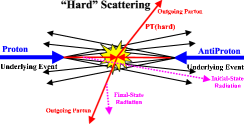
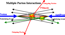
The “beam-beam remnants” are what is left over after a parton is knocked out of each of the initial two beam hadrons. It is the reason hadron-hadron collisions are more “messy” than electron-positron annihilations and no one really knows how it should be modeled. For the QCD Monte-Carlo models the “beam-beam remnants” are an important component of the “underlying event”. Also, it is possible that multiple parton scattering contributes to the “underlying event”. Fig. 10 shows the way PYTHIA [23, 24, 1] models the “underlying event” in proton-antiproton collisions by including multiple parton interactions. In addition to the hard -to- parton-parton scattering and the “beam-beam remnants”, sometimes there is a second “semi-hard” -to- parton-parton scattering that contributes particles to the “underlying event”.
Of course, from a certain point of view there is no such thing as an “underlying event” in a proton-antiproton collision. There is only an “event” and one cannot say where a given particle in the event originated. On the other hand, hard scattering collider “jet” events have a distinct topology. On the average, the outgoing hadrons “remember” the underlying the -to- hard scattering subprocess. An average hard scattering event consists of a collection (or burst) of hadrons traveling roughly in the direction of the initial beam particles and two collections of hadrons (i.e., “jets”) with large transverse momentum. The two large transverse momentum “jets” are roughly “back-to-back” in azimuthal angle. One can use the topological structure of hadron-hadron collisions to study the “underlying event” [22, 25, 26, 27, 28, 29]. Here we study the “underlying event” in the Run using the direction of the leading calorimeter jet (JetClu, ) to isolate regions of - space that are sensitive to the “underlying event”.
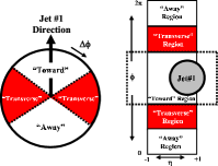
As illustrated in Fig. 11, the direction of the leading jet, jet# , is used to define correlations in the azimuthal angle, . The angle is the relative azimuthal angle between a charged particle and the direction of jet# . The “toward” region is defined by and , while the “away” region is and . The “transverse” region is defined by and . The three regions “toward”, “transverse”, and “away” are shown in Fig. 11. Each region has an area in -space of . The “transverse” region is perpendicular to the plane of the hard -to- scattering and is therefore very sensitive to the “underlying event”. We restrict ourselves to charged particles in the range and , but allow the leading jet that is used to define the “transverse” region to have .
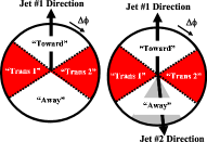
In this analysis we look in more detail at the two “transverse” regions defined in Fig. 12. The overall “transverse” region in Fig. 11 corresponds to combining the “transverse ” and “transverse ” regions. Comparing these two “transverse” regions on an event-by-event basis provides a closer look at the “underlying event”. Here we refer to events in which there are no restrictions placed on the second highest jet, jet#, as “leading jet” events. Our previous analysis of the “underlying event”we only considered “leading jet” events [22, 27, 28, 29]. In this analysis we define a second class of events. Events with at least two jets with , where the leading two jets are nearly “back-to-back” () with are referred to as “back-to-back” events. “Back-to-back” events are a subset of the “leading jet” events. The idea here is to suppress hard initial and final-state radiation thus increasing the sensitivity of the “transverse” region to the “beam-beam remnants” and the multiple parton scattering component of the “underlying event”.
As in our published Run 1 analysis [22] we consider charged particles only in the region and where the COT efficiency is high and compare uncorrected data with PYTHIA Tune A [27, 28] and HERWIG [30, 31, 32] after detector corrections (i.e., CDFSIM). Systematic errors are calculated in the same way as in our Run 1 analysis. We generate every plot twice, once with our chosen track selection cuts and again with the very tight track cuts. The change in each point in every plot due to this tighter cut is used as a measure of the systematic error and is added in quadrature with the statistical error to form the overall error.
5.2 Transverse Average vs
5.2.1 Definition
We study the average transverse momentum of charged particles in the “transverse” region as a function of the number of charged particles in the “transverse” region for and . The average transverse momentum, , is formed, on an event-by-event basis, and then plotted as a function of the charged multiplicity. The idea here is to look for correlations between multiplicity and . If, for example, there is a mixture of “hard” and “soft” events then one expects that will increase with multiplicity because demanding a large multiplicity will preferentially select the “hard” process that also has a larger . On the other hand, it may be possible to get a high multiplicity in a “soft” collision so the rate that rises with multiplicity is a rough measure of the “hard” and “soft” mixture. The steeper the slope the larger the “hard” component. There is a very nice published CDF Run 1 analysis that looks at this in “min-bias” collisions [33], but it has never previously been studied in the “transverse” region of a “hard” scattering process.
5.2.2 Overall Transverse Region
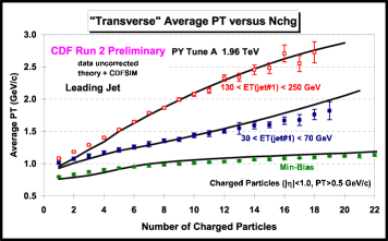
Fig. 13 shows uncorrected Run 2 data on the of charged particles versus the number of charged particles in min-bias collisions and in the “transverse” region for “leading jet” events with and compared with PYTHIA Tune A (after CDFSIM). The data suggest that there is more “hard” scattering in the “transverse” region (i.e., initial and final-state radiation) than there is in an average “min-bias” collision.
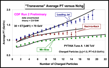
Fig. 14 shows the of charged particles versus the number of charged particles in “min-bias” collisions and in the “transverse” region for “leading jet” and “back-to-back” events with compared with PYTHIA Tune A (after CDFSIM). The “transverse” region for the “back-to-back” events looks more like an average “min-bias” collision, which is exactly what one expects since the “back-to-back” requirement suppress hard initial and final-state radiation.
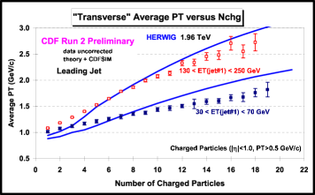
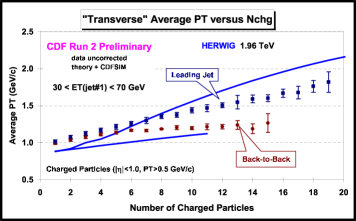
Fig. 15 compares HERWIG (after CDFSIM) with the data on the of charged particles in the “transverse” region versus the number of charged particles in the “transverse” region for “leading jet” events with and .
Fig. 16 compares HERWIG (after CDFSIM) with the data on the of charged particles in the “transverse” region versus the number of charged particles in the “transverse” region for “leading jet” and “back-to-back” events with . HERWIG (without multiple parton interactions) does not describe the data as well as PYTHIA Tune A (with multiple parton interactions).
5.2.3 Transverse 1 versus transverse 2
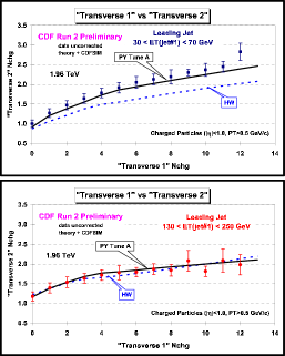
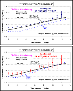
Fig. 17 shows the number of charged particles in the “transverse ” region versus the number of charged particles in the “transverse ” region for “leading jet” events with and compared with PYTHIA Tune A and HERWIG after CDFSIM.
Fig. 18 shows the of charged particles in the “transverse ” region versus the number of charged particles in the “transverse ” region for “leading jet” events with and compared with PYTHIA Tune A and HERWIG after CDFSIM.
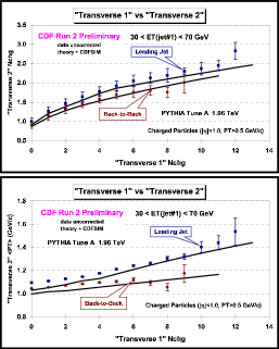
Fig. 19 shows the number and of charged particles in the “transverse ” region versus the number of charged particles in the “transverse ” region for “leading jet” and “back-to-back” events with compared with PYTHIA Tune A (after CDFSIM).
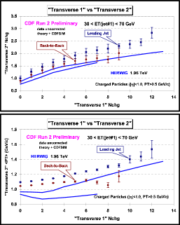
Fig. 20 shows the number and of charged particles in the “transverse ” region versus the number of charged particles in the “transverse ” region for “leading jet” and “back-to-back” events with compared with HERWIG (after CDFSIM). HERWIG (without multiple parton interactions) does not do nearly as well describing the “transverse ” versus “transverse ” correlations seen in the data as does PYTHIA Tune A (with multiple parton interactions).
5.3 Summary
This analysis takes a closer look at the “underlying event” in hard scattering proton-antiproton collisions at . We look only at the charged particle component of the “underlying event” and restrict the charged particles to be in the range and . We use the direction of the leading calorimeter jet in each event to define two “transverse” regions of - space that are very sensitive to the “underlying event”. Comparing these two “transverse” regions on an event-by-event basis provides more details about the “underlying event”. In addition, by selecting events with at least two jets that are nearly “back-to-back” () we are able to look closer at the “beam-beam remnants” and multiple parton interaction components of the “underlying event”. PYTHIA Tune A (with multiple parton interactions) does a good job in describing the “underlying event” (i.e., “transverse” regions) for both “leading jet” and “back-to-back” events. HERWIG (without multiple parton interactions) does not have enough activity in the “underlying event”, which was also observed in our published Run 1 analysis [22].
The data presented here show interesting correlations between the two “transverse” regions defined in Fig. 12. The charged multiplicity and the in the “transverse ” region increases with the charged multiplicity in the “transverse ” region. This is a new type of correlation. It might simply be due to a high multiplicity in “transverse ” biasing in favor of a harder -to- scattering (i.e., higher ) which would result in a higher multiplicity and larger in “transverse ”. However, we have seen in previous studies [22, 25, 26, 27, 28, 29] that the average charged particle density in the “transverse” region does not change much as one increases . It is possible that the “transverse ” versus “transverse ” correlations arise from multiple parton interactions. A large multiplicity in the “transverse ” region would indicate a small impact parameter collision has occurred with several multiple parton scatterings which would then cause an increased multiplicity and in the “transverse ” region. The fact that PYTHIA Tune A (with multiple parton interactions) agrees with the data better than HERWIG (without multiple parton interactions) is very interesting. However, much more work is necessary to actually pinpoint the source of the “transverse ” versus “transverse ” correlations.
6 SIMULATION OF THE QCD BACKGROUND FOR ANALYSES AT THE TEVATRON WITH A JETS FINAL STATE 555Contributed by: V. Drollinger
6.1 Introduction
The top quark mass and the cross section of top quark pair production are important measurements at the Tevatron. Compared to Run I, the precision of these measurements is expected to be much higher in Run II Ref. [34]. This requires an accurate understanding of all the important backgrounds. In the semileptonic top decay channel with one lepton and four jets plus missing energy in the final state, the QCD background is one of the main backgrounds. The cross section of this background is large compared to the cross section of production, but can be reduced strongly with appropriate selection criteria. In the past, this background was modeled using events with non-isolated leptons coming from experimental data. It is however important that in analyses with final states the lepton is isolated in order to reduce backrounds with non-isolated leptons. It is not possible to get a clean sample of QCD events with isolated leptons directly from the data since these would be mixed with and events. Therefore, in the following, we instead model the QCD background via Monte Carlo with and production and subsequent leptonic -decay.
6.2 Simulation Procedure
-
Hard Process: the hard process is generated with ALPGEN Ref. [35]. The final state consists of a pair together with two other partons (light quarks or gluons). In the following, these events are referred to as “bb2j” events. They are generated with , , and . In order to produce the events in kinematically interesting regions, we apply the following phase space cuts for all four partons, including the and : , and . In addition, we require at least one -quark with a transverse momentum bigger than 30 in order to provide phase space for the leptonic -decay. The bb2j cross section including these cuts is about 30 .
-
Fragmentation: during the fragmentation with PYTHIA Ref. [10] a high electron or muon is produced in a leptonic -decay. In order to increase the number of events with energetic leptons, the fragmentation is repeated exactly forty times. For this number of repetitions, we obtain about one event with a high lepton. A constant number of repetitions should not bias the spectrum of the lepton. Events preselected with a lepton with of at least 15 are written to a HEPEVT file. The high lepton requirement reduces the cross section to 14.5 (288864 events, the first number in Table 2 below), presumably with a large theoretical uncertainty666The cross section of bb2j is calculated at leading order. Additional background contributions from similar processes like cc2j are not included..
-
CDF detector simulation: The standard CDF software package reads the HEPEVT file, and performs a detailed simulation of the CDF detector response. After the simulation, the events are reconstructed with the same algorithms as used to reconstruct the Run II data. Finally, the top working group‘s standard ntuple is written which we examine in the following.
6.3 Comparison with Data
-
Preselection: we select events with exactly one lepton777We use the CDF baseline selection criteria for high quality lepton identification without the isolation cut. Events with cosmic muons or more than one lepton are rejected as well. with 20 and with missing transverse energy of at least 20 . Furthermore, we ask for at least four jets with and . Three jets per event are required to be high quality jets with and . In addition, we remove events with more than two -quarks in case of simulated events. This mitigates a potential bias888The repetition of the fragmentation would cause an artificial enhancement of additional pairs coming from gluon splitting with subsequent leptonic -decay. from the repetition of the fragmentation. In case of the data, we use good runs only.
-
QCD region: in the plane of the lepton isolation variable 999The lepton isolation variable is defined as the fractional calorimeter isolation in a cone of 0.4 around the lepton. and the distance of the lepton to the closest jet we select a region, where we expect almost purely QCD events in the data. In this region the lepton is non-isolated and is well inside a jet: and . Isolated leptons coming from real decays, are found typically at low and at any value of which means, those leptons are usually isolated and also separated from jets.
-
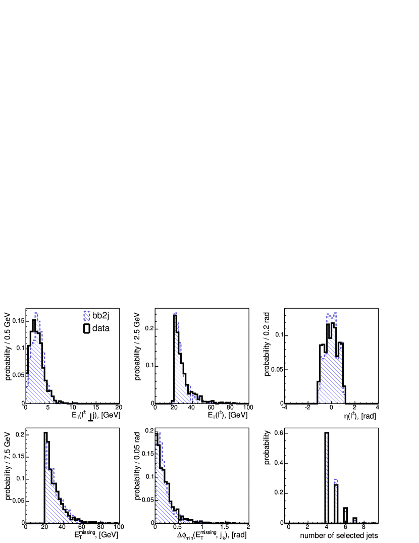
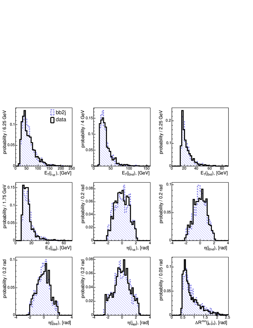
Comparison: in order to evaluate the simulated bb2j event simulation, we compare the events in the QCD region with events from the data which have undergone the same preselection. The data sets are called btop0g, btop1g, btop0j, and btop1j with the number of events listed in Table 2. All events correspond to an integrated luminosity of 126 . In case of the simulated bb2j events ”all events” is the number of events after the full simulation and reconstruction. We compare the most relevant kinematic variables in Figs. 22 and 21.
| event type | bb2j | data |
|---|---|---|
| all events | 288864 | 955870 |
| preselection | 846 | 1669 |
| QCD region | 666 | 1043 |
In order to validate the simulation of bb2j events, we have studied the shapes of kinematic distributions. Whereas the jets (Fig. 22) are more related to the hard QCD process, the lepton and the neutrino, seen as missing , (Fig. 21) depend rather on the -decay and fragmentation, respectively. However, the kinematic properties of the jets, the lepton, and the neutrino are correlated. There are no major differences between simulated bb2j events and the CDF data.
6.4 Summary
Top physics at the Tevatron has entered the Run II phase with high luminosity and upgraded detectors, and therefore the measurements obtained in the top sector will reach much higher precision. This requires a good understanding of all relevant background processes. The use of new Monte Carlo tools enable us to simulate the QCD background.
We have described the bb2j event generation procedure. After the hard process with four partons in the final state is generated with ALPGEN, the high lepton is obtained from a leptonic -decay during the fragmentation with PYTHIA.
We define a region, where we expect to have a clean QCD sample and compare the fully simulated events with the CDF Run II data. All of the kinematic variables studied, compare well. From this comparison we conclude, that bb2j events can be used to model the QCD background with a final state.
Acknowledgments
We would like to thank Michelangelo Mangano and Torbjörn Sjöstrand for very useful comments and suggestions concerning the generation of bb2j events. Many thanks to Michael Gold and Dmitri Smirnov for helping to prepare this article.
7 MONTE-CARLO DATABASE 101010Contributed by: L. Dudko and A. Sherstnev
7.1 Problem description
One of the most general problems for the experimental high energy physics community is Monte-Carlo (MC) simulation of physics processes. There are numerous publicly available MC generators. However, the correct MC simulation of complicated processes requires in general rather sophisticated expertise on the part of their users. Often, a physics group in an experimental collaboration requests experts and/or authors of MC generators to create MC samples for a particular process. Furthermore, it is common that the same physics process is investigated by various physics groups in need of the the same MC event samples. The main motiviation behind the Monte-Carlo Database (MCDB) project is to make MC event samples, as prepared by experts, available for various physics groups. In this contribution we present a version of the MCDB that is already operative in the CMS collaboration, and discuss future plans.
There are a number of useful aspects to a central MC Database that motivate its establishment.
-
1.
Correct and reliable MC event generation of most processes of interest requires considerable expertise. Moreover, most MC generators, in particular those calculating higher order perturbative corrections, require significant amounts of computer resources. By means of the MCDB, samples prepared by experts can be distributed easily and used as many times as needed.
-
2.
Public availability of common event files helps speed up the validation procedure of the events.
-
3.
A central and public location where well-documented MC events and MC generators can be found would be very useful. It would also allow rapid communication between authors of MC events and their users.
-
4.
The same MC samples for SM processes can be used for multiple purposes, e.g. to study backgrounds to various new physics processes.
-
5.
Files containing detector and beam-related backgrounds can also be kept in a common location.
7.2 History
The first MC Database (version 0) – named PEVLIB [36] – was established at CERN, on the AFS file-system. This database provided CompHEP [37] parton level events for CMS users, but lacked a special interface. Rather, it was built as a set of directories where event samples were stored. The sample documentation consisted of ASCII files (README) located in the same directories as the event files.
The next version (version 0.5) of the MC Database was established at Fermilab. This database was split in two independent parts:
The latest version of the MCDB (version 1.0), described in this contribution, CMS MCDB [40], was created at first for use by the CMS collaboration. This database includes web interfaces both for event files (enabling download and upload) and documentation. Its main goal is to store events, only at the parton level, generated by MC experts, for use by the LHC community. Note that all files from PEVLIB have now been moved to the CMS MCDB.
7.3 General concepts and practical realization of CMS MCDB.
The MCDB must provide persistent storage of event samples, with public and convenient interfaces for users – mainly consisting of LHC experimentalists – and authors of MC generators, or other experts. The main features present in the CMS MCDB are:
-
the MCDB is based on web technologies.
-
the MCDB stores parton level events with a standard interface to the next level of simulation (based on Les Houches Accord I).
-
the MCDB stores detailed documentation for each set of event samples.
-
the MCDB make rapid communication between users and experts possible via its web pages.
-
the MCDB is divided in two zones:
-
a public area, for all users interested in using MC events. Users can find all necessary information about available event samples and their generators, and download the corresponding event files.
-
a restricted area for authors. In this area, authors of MC generators or MC experts can change the content of MCDB dynamically – e.g. upload events for new processes, create and edit documents, reply to user’s comments and questions and upload new event files and generators.
-
-
the MCDB requires users to reference the authors of the event sample in case the events are used in a physics analysis.
The CMS MCDB at CERN is realized as a dedicated web site [40]. The structure of the site corresponds to the stored physics processes. For example, all event files relevant for studies of top quark production are collected in the category “TOP”. This category contains files with events involving top quark production via QCD and the electroweak interaction. When a user clicks on a reference in a certain category, he/she will see all so-called ”articles” related to the selected physics process.
The main units of CMS MCDB are HTML documents called articles that describe the event samples. The articles are created by authors; these are authorized users who can upload new event samples to the CMS MCDB. There are only a few restrictions on the articles in the CMS MCDB. An author can create a new article on the basis of a template – this is a web form, where the author fills out various fields: author name, abstract, category name, article body, etc. The body and the abstract of the article may include HTML tags for more flexible visualization.
It is easy for users to understand which process is present in the CMS MCDB, via a click on a reference to the article that describes the corresponding event samples. Users can download these event files directly from the article web page, together with all other files which authors have uploaded to the article.
The web intereface of the present version of the MCDB has the following features, in brief:
A. Authorized authors can
-
upload files (with events or a MC generator code). There are two different methods to upload file (through a web browser and/or directly from the AFS file system).
-
document each set of files in a new article.
-
reply to comments from users (MCDB allows one to organize a special forum for each article).
-
change any of the parameters and content of MCDB, according to permissions (including the web design).
B. Users can
-
read documentation (MCDB articles) for files uploaded by authors.
-
download files.
-
search the CMS MCDB web site (enabled for articles only, not for the event samples themselves).
-
ask questions about a particular document.
-
send new articles to moderators.
Event files in the CMS MCDB are stored on the AFS filesystem [41]. If a user has access to AFS, he/she may download files from AFS directly. To become an authorized author one should send a request (by e-mail) to the administrators 111111A. De Roeck (Albert.de.Roeck@cern.ch), L. Dudko (Lev.Doudko@cern.ch), S. Slabospitsky (Sergey.Slabospitsky@cern.ch) and A. Sherstnev (Alexandre.Cherstnev@cern.ch) of the CMS MCDB.
7.4 Future plans
The CMS MCDB is designed to store parton level events. This implies that the size of event files should not be too large (typically smaller then 100Mb). The expected number of physics processes in the CMS MCDB is several hundred. Note that CMS MCDB is not a SQL database, so that its search engine cannot serve complex queries, only keyword phonetic searches. These aspects of the CMS MCDB are not a limitation at present. However, we expect that in a few years users will request a more powerful MCDB where these restrictions will be removed. The next version of the MCDB now under development for use, within the CERN LCG framework, by all CERN collaborations. It will be described in the near future [42].
Acknowledgements
L. Dudko would like to thank INTAS for their financial support (YSF-2002-239 and RF President grant MK-1954.2003.02) of the MCDB project.
8 RESUMMATION AND SHOWER STUDIES 121212Contributed by: J. Huston, I. Puljak, T. Sjöstrand, E. Thomé
8.1 Introduction
The transverse momentum of a colour-singlet massive particle produced in a hadronic collision provides important information on perturbative and nonperturbative effects. A process like corresponds to , while higher-order processes provide kicks as the recoils against quarks and gluons. At large values the bulk of the comes from one hard emission, and perturbation theory is a reasonable approach. In the small- region, on the other hand, many emissions can contribute with kicks of comparable size, and so the order-by-order approach is rather poorly convergent. Furthermore, in this region nonperturbative effects may start to become non-negligible relative to the perturbative ones.
The traditional solution has been to apply either an analytical resummation approach or a numerical parton-shower one. These methods to some extent are complementary. The norm today is for showers to be based on an improved leading-log picture, while resummation is carried out to next-to-leading logs. However, resummation gives no information on the partonic system recoiling against the , while showers do, and therefore can be integrated into full-fledged event generators, allowing accurate experimental studies. In both approaches the high- tail is constrained by fixed-order perturbation theory, so the interesting and nontrivial region is the low-to-medium- one. Both also require nonperturbative input to handle the low- region, e.g. in the form of a primordial carried by the initiator of a shower.
One of the disconcerting aspects of the game is that a large primordial seems to be required and that the required value of this primordial can be dependent on the kinematics of the process being considered. Confinement of partons inside the proton implies a GeV, while fits to data at the Tevatron favour GeV [43] (actually as a root-mean-square value, assuming a Gaussian distribution). Also resummation approaches tend to require a non-negligible nonperturbative contribution, but that contribution can be determined from fixed-target data and then automatically evolved to the kinematical region of interest. In this note we present updated comparisons and study possible shower modifications that might alleviate the problem. We will use the two cases of and (in the infinite-top-mass limit) to illustrate differences in quark and gluon evolution, and the Tevatron and the LHC to quantify an energy dependence.
8.2 Comparison Status
A detailed comparison of analytic resummation and parton showers was presented in [43]. For many physical quantities, the predictions from parton shower Monte Carlo programs should be nearly as precise as those from analytical theoretical calculations. In particular, both analytic and parton shower Monte Carlos should accurately describe the effects of the emission of multiple soft gluons from the incoming partons.
Parton showers resum primarily the leading logs, which are universal, i.e. process-independent, depending only on the initial state. An analytic resummmation calculation, in principle, can resum all logs, but in practice the number of towers of logarithms included in the analytic Sudakov exponent depends on the level to which a fixed-order calculation was performed for a given process. Generally, if a NNLO calculation is available, then the coefficient (using the CSS formalism [44]) can be extracted and incorporated. If we try to interpret parton showering in the same language then we say that the Monte Carlo Sudakov exponent always contains a term analogous to and and that an approximation to is also present in some kinematic regions.
In Ref. [43], predictions were made for both and Higgs production at the Tevatron and the LHC, using both resummation and parton shower Monte Carlo programs. In general, the shapes for the distributions agreed well, although the Pythia showering algorithm typically caused the Higgs distribution to peak at somewhat lower values of transverse momentum.
8.3 Shower Algorithm Constraints
While customarily classified as leading log, shower algorithms
tend to contain elements that go beyond the conventional leading-log
definition. Specifically, some emissions allowed by leading log
are forbidden in the shower description. Taking the Pythia
[10, 7] initial-state shower algorithm
[23, 24, 45] as an example,
the following aspects may be noted (see [46] for
further details):
(i) Emissions are required to be angularly ordered, such that
opening angles increase on the way in to the hard scattering subprocess.
That is, non-angularly-ordered emissions are vetoed.
(ii) The and of a branching are required
to fulfill the condition . Here
, for the incoming parton
on the other side of the event. In the case that and form a
, say, and is the recoiling parton,
coincides with the standard Mandelstam variable for the
process. In general, it may be
viewed as a kinematics consistency constraint.
(iii) The evolution rate is proportional to
rather than
. Since this
implies by itself a larger and thus an increased rate of
evolution. However, one function of the GeV
nonperturbative cutoff parameter is to avoid the
divergent- region, so now one must require
rather than . The net result again
is a reduced emission rate.
(iv) One of the partons of a branching may develop a timelike
parton shower. The more off-shell this parton, the less the
of the branching. The evolution rate in is unaffected, however.
(v) There are some further corrections, that in practice appear
to have negligible influence: the non-generation of very soft gluons to
avoid the divergence of the splitting kernel, the possibility of photon
emission off quarks, and extra kinematical constraints when heavy quarks
are produced.
(vi) The emission rate is smoothly merged with the first-order
matrix elements at large . This is somewhat separate from
the other issues studied, and the resulting change only appreciably
affects a small fraction of the total cross section, so it will not be
considered further here.
The main consequence of the first three points is a lower rate of evolution. That is, starting from a set of parton densities at some low scale, and a matching , tuned such that standard DGLAP evolution provides a reasonable fit to data at , the constraints above lead to distributions less evolved and thus harder than data. If we e.g. take the CTEQ5L tune [47] with GeV, the would need to be raised to about 0.23 GeV in the shower to give the same fit to data as CTEQ5L when the angular-ordering cut in (i) is imposed. Unfortunately effects from points (ii) and (iii) turn out to be process-dependent, presumably reflecting kinematical differences between and . There is also some energy dependence. The net result of the first three points suggests that Pythia should be run with a of about 0.3 GeV (0.5 GeV) for () production in order to compensate for the restrictions on allowed branchings.
One would expect the increased perturbative evolution to allow the primordial to be reduced. Unfortunately, while the total radiated transverse energy, , comes up by about 10% at the Tevatron, this partly cancels in the vector sum, . For a 2 GeV primordial the shift of the peak position of the spectrum is negligible. Results are more visible for at the LHC.
Note that a primordial assigned to the initial parton at the low scale is shared between the partons at each shower branching, in proportion to the longitudinal momentum fractions a daughter takes. Only a fraction of the initial thus survives to the hard-scattering parton. Since the typical evolution range is much larger at the LHC than at the Tevatron, a tuning of the primordial is hardly an option for at the LHC, while it is relevant for at the Tevatron. Therefore an increased value is an interesting option.
We now turn to the point (iv) above. By coherence arguments, the main chain of spacelike branchings sets the maximum virtuality for the emitted timelike partons, i.e. the timelike branchings occur at longer timescales than the related spacelike ones. In a dipole-motivated language, one could therefore imagine that the recoil, when a parton acquires a timelike mass, is not taken by a spacelike parton but by other final-state colour-connected partons. A colour-singlet particle, like the or , would then be unaffected by the timelike showers.
The consequences for and of such a point of view can be studied by switching off timelike showers in Pythia, but there is then no possibility to fully simulate the recoiling event. A new set of shower routines is in preparation [48], however, based on -ordered emissions in a hybrid between conventional showers and the dipole approach. It is well suited for allowing final-state radiation at later times, leaving and unaffected at that stage. Actually, without final-state radiation, the two approaches give surprisingly similar results overall. Both are lower in the peak region than the algorithm with final-state radiation, in better agreement with CDF data [49]. The new one is slightly lower, i.e. better relative to data, at small values.
A combined study [46], leaving both the primordial and the value free, still gives some preference to GeV and the standard GeV, but differences relative to an alternative with GeV and GeV are not particularly large, Fig. 23.

8.4 Further Comparisons
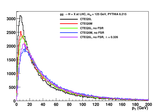
Returning to Higgs production at the LHC, in Fig. 24 are shown a number of predictions for the current standard Pythia shower routines. Using CTEQ5M rather than CTEQ5L results in more gluon radiation and a broader distribution due to the large value of . Likewise turning off timelike showers for gluons radiated from the initial state also results in the peak of the distribution moving outwards.
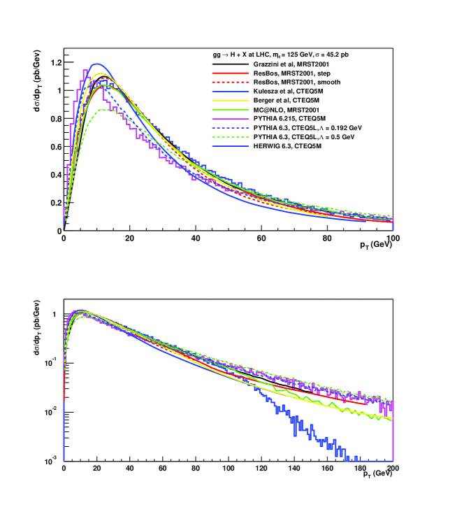
We can now compare the results with resummation descriptions and other generators, Fig. 25 [50]. As we see, the new Pythia routines agree better with resummation descriptions than in the past [43], attesting to the importance of various minor technical details of the Monte Carlo approach. One must note, however, that some spread remains, and that it is not currently possible to give an unambiguous prediction.
8.5 Conclusions
We have studied and spectra, as a way of exploring perturbative and nonperturbative effects in hadronic physics. Specifically, we have pointed out a number of ambiguities that can exist in a shower approach, e.g. that the shower goes beyond the simpleminded leading-log evolution and kinematics, while still making use of leading-log parton densities. Attempts to correct for mismatches in general tend to increase the perturbative . The need for an unseemly large primordial in the shower approach is thus reduced, but not eliminated. There is still room for, possibly even a need of, perturbative evolution beyond standard DGLAP at small virtuality scales.
9 NEW SHOWERS WITH TRANSVERSE-MOMENTUM-ORDERING 131313Contributed by: T. Sjöstrand
9.1 Introduction
The initial- [23, 24, 45] and final-state [58, 59] showers in the Pythia event generator [10, 7] are based on virtuality-ordering, i.e. uses spacelike and timelike , respectively, as evolution variables. Other algorithms in common use are the angular-ordered ones in Herwig [60, 57] and the -ordered dipole-based ones in Ariadne/Ldc [61, 62]. All three have been comparably successful, in terms of ability to predict or describe data, and therefore have offered useful cross-checks. Some shortcomings of the virtuality-ordering approach, with respect to coherence conditions, have been compensated (especially relative to Herwig) by a better coverage of phase space and more efficient possibilities to merge smoothly with first-order matrix elements.
Recently, the possibility to combine matrix elements of several orders consistently with showers has been raised [63, 64], e.g. jets, . In such cases, a -ordering presumably offers the best chance to provide a sensible definition of hardness. It may also tie in better e.g. with the -ordered approach to multiple interactions [65]. This note therefore is a study of how the existing Pythia algorithms can be reformulated in -ordered terms, while retaining their strong points.
The main trick that will be employed is to pick formal definitions of , that simply and unambiguously can be translated into the older virtuality variables, e.g. for standard matrix-element merging. These definitions are based on lightcone kinematics, wherein a timelike branching into two massless daughters corresponds to and the branching of a massless mother into a spacelike and a massless daughter to . The actual of a branching will be different, and e.g. depend on the subsequent shower history, but should normally not deviate by much.
9.2 Timelike Showers
The new timelike algorithm is a hybrid between the traditional parton-shower and dipole-emission approaches, in the sense that the branching process is associated with the evolution of a single parton, like in a shower, but recoil effects occur inside dipoles. That is, a dipole partner is assigned for each branching, and energy and momentum is ‘borrowed’ from this partner to give mass to the parton about to branch, while preserving the invariant mass of the dipole. (Thus four-momentum is not preserved locally for each parton branching . It was in the old algorithm, where the kinematics of a branching was not constructed before the off- or on-shell daughter masses had been found.) Often the two partners are colour-connected, i.e. the colour of one matches the anticolour of the other, as defined by the preceding showering history, but this need not be the case. In particular, intermediate resonances normally have masses that should be preserved by the shower, e.g., in the takes the recoil when the radiates a gluon.
The evolution variable is approximately the of a branching, where is the transverse momentum for each of the two daughters with respect to the direction of the mother, in the rest frame of the dipole. (The recoiling dipole partner does not obtain any kick in this frame; only its longitudinal momentum is affected.) For the simple case of massless radiating partons and small virtualities relative to the kinematically possible ones, and in the limit that recoil effects from further emissions can be neglected, it agrees with the -clustering distance defined in the PYCLUS algorithm [66].
All emissions are ordered in a single sequence . That is, each initial parton is evolved from the input scale downwards, and a hypothetical branching is thereby found for it. The one with the largest is chosen to undergo the first actual branching. Thereafter, all partons now existing are evolved downwards from , and a is chosen, and so on, until is reached. (Technically, the values for partons not directly or indirectly affected by a branching need not be reselected.) The evolution of a gluon is split in evolution on two separate sides, with half the branching kernel each, but with different kinematical constraints since the two dipoles have different masses. The evolution of a quark is also split, into one scale for gluon emission and one for photon one, in general corresponding to different dipoles.
With the choices above, the evolution factorizes. That is, a set of successive calls, where the of one call becomes the of the next, gives the same result (on the average) as one single call for the full range. This is the key element to allow Sudakovs to be conveniently obtained from trial showers [64], and to veto emissions above some scale, as required to combine different -parton configurations efficiently.
The formal definition is , where is the evolution variable, gives the energy sharing in the branching, as selected from the branching kernels, is the off-shell mass of the branching parton and its on-shell value. This is also used as scale.
When a has been selected, this is translated to a . Note that the Jacobian factor is trivial: . From there on, the three-body kinematics of a branching is constructed as in the old routine. This includes the detailed interpretation of and the related handling of nonzero on-shell masses for branching and recoiling partons, which leads to the physical not agreeing with the defined here. In this sense, becomes a formal variable, while really is a well-defined mass of a parton.
Also the corrections to branchings ( being a generic coloured particle) by merging with first-order matrix elements closely follows the existing machinery [59], once the has been converted to a mass of the branching parton. In general, the other parton used to define the matrix element need not be the same as the recoiling partner. To illustrate, consider a decay. Say the branches first, . Obviously the then takes the recoil, and the new , and momenta are used to match to the matrix element. The next time branches, , the recoil is taken by the colour-connected gluon, but the matrix element corrections are based on the newly created and momenta together with the (not the !) momentum. That way one may expect to achieve the most realistic description of mass effects in the collinear and soft regions.
The shower inherits some further elements from the old algorithm, such as azimuthal anisotropies in gluon branchings from polarization effects.
The relevant parameters will have to be retuned, since the shower is quite different from the old mass-ordered one. In particular, it appears that the five-flavour value has to be reduced relative to the current default, roughly by a factor of two (from 0.29 to 0.14 GeV).
9.3 Spacelike Showers
Initial-state showers are constructed by backwards evolution [23], starting at the hard interaction and successively reconstructing preceding branchings. To simplify the merging with first-order matrix elements, is defined by the ratio of before and after an emission. For a massless parton branching into one spacelike with virtuality and one with mass , this gives , or for . Here is the squared invariant mass after the emission, i.e. excluding the emitted on-mass-shell parton.
The last term, , while normally expected to be small, gives a nontrivial relationship between and , e.g. with two possible solutions for a given . To avoid the resulting technical problems, the evolution variable is picked to be . Also here sets the scale for the running . Once selected, the is translated into an actual by the inverse relation , with trivial Jacobian: . From the correct , including the term, can be constructed.
Emissions on the two incoming sides are interspersed to form a single falling sequence, . That is, the of the latest branching considered sets the starting scale of the downwards evolution on both sides, with the next branching occurring at the side that gives the largest such evolved .
In a branching , the newly reconstructed mother is assumed to have vanishing mass — a heavy quark would have to be virtual to exist inside a proton, so it makes no sense to put it on mass shell. The previous mother , which used to be massless, now acquires the spacelike virtuality and the correct previously mentioned, and kinematics has to be adjusted accordingly.
In the old algorithm, the kinematics was not constructed until its spacelike virtuality had been set, and so four-momentum was explicitly conserved at each shower branching. In the new algorithm, this is no longer the case. (A corresponding change occurs between the old and new timelike showers, as noted above.) Instead it is the set of partons produced by this mother and the current mother on the other side of the event that collectively acquire the of the new branching. Explicitly, when the is pushed off-shell, the four-momentum is modified accordingly, such that their invariant mass is retained. Thereafter a set of rotations and boosts of the whole -produced system bring them to the frame where has the desired and is restored to its correct four-momentum.
Matrix-element corrections can be applied to the first, i.e. hardest in , branching on both sides of the event, to improve the accuracy of the high- description. Also several other aspects are directly inherited from the old algorithm.
Work on the algorithm is ongoing. In particular, an optimal description of kinematics for massive quarks in the shower, i.e. and quarks, remains to be worked out.
Some first tests of the algorithm are reported elsewhere [67]. In general, its behaviour appears rather similar to that of the old algorithm.
9.4 Outlook
The algorithms introduced above are still in a development stage. In particular, it remains to combine the two. One possibility would be to construct the spacelike shower first, thereby providing a list of emitted partons with their respective emission scales. This list would then be used as input for the timelike shower, where each emission sets the upper evolution scale of the respective parton. This is straightforward, but does not allow a fully factorized evolution, i.e. it is not feasible to stop the evolution at some value and continue downwards from there in a subsequent call. The alternative would be to intersperse spacelike and timelike branchings, in one common -ordered sequence.
Obviously the finished algorithms have to be compared with data, to understand how well they do. One should not expect any major upheavals, since checks show that they perform similarly to the old ones at current energies, but the hope is for a somewhat improved and more consistent description. The step thereafter would be to study specific processes, such as jets, to find how good a matching can be obtained between the different -jet multiplicities, when initial parton configurations are classified by their -clustering properties. The PYCLUS algorithm here needs to be extended to cluster also beam jets. Since one cannot expect a perfect match between generated and clustering-reconstructed shower histories, it may become necessary to allow trial showers and vetoed showers over some matching range, but hopefully then a rather small one. If successful, one may expect these new algorithms to become standard tools for LHC physics studies in the years to come.
10 MATCHING MATRIX ELEMENTS AND PARTON SHOWERS WITH HERWIG AND PYTHIA 141414Contributed by: S. Mrenna
10.1 Introduction
Parton-shower (PS) Monte Carlo event generators are an important tool in the experimental analyses of collider data. These computational programs are based on the differential cross sections for simple scattering processes (usually particle scatterings) together with a PS simulation of additional QCD radiation that naturally connects to a model of hadronization. As the PS algorithms are based on resummation of the leading soft and collinear logarithms, these programs may not reliably estimate the radiation of hard jets, which, in turn, may bias experimental analyses.
Improvements have been developed to correct the emission of the hard partons in the PS. In PYTHIA [10, 11, 7], corrections were added for annihilation [68], deep inelastic scattering [69], heavy particle decays [59] and vector boson production in hadron-hadron collisions [45]. Similarly, corrections were added to HERWIG [57, 70] in Refs. [71, 72, 73, 74] following the method described in [75].
The Catani-Krauss-Kuhn-Webber (CKKW) algorithm is a method for generalizing such corrections [63, 76]. Along with this development, computer programs have become available [77, 35] which are capable of efficiently generating multi-parton events in a format (the Les Houches format[78]) that can be readily interfaced with HERWIG and PYTHIA. Here, we report on how to use these programs combined with the HERWIG and PYTHIA Monte Carlo event generators to implement hard corrections to PS predictions. Several approaches are explored. One adheres closely to the CKKW algorithm, but uses HERWIG for adding an additional PS. The second is more closely tuned to the specific PS generators themselves and calculates branching probabilities numerically (using exact conservation of energy and momentum) instead of analytically. This is accomplished by generating pseudo-showers starting from the various stages of a PS history. A comparison is also made with a much simpler method.
10.2 Overview of the Correction Procedure
PS’s are used to relate the partons produced in a simple, hard interaction characterized by a large energy scale (large means ) to the partons at an energy scale near . At this lower scale, a transition is made to a non–perturbative description of hadronic physics, with physical, long–lived particles as the final products. This is possible, because the fragmentation functions for the highly-virtual partons obey an evolution equation that can be solved analytically or numerically. This solution can be cast in the form of a Sudakov form factor, which can be suitably normalized as a probability distribution for no parton emission between two scales. Using the Monte Carlo method, the evolution of a parton can be determined probabilistically, consisting of steps when the parton’s scale decreases with no emission, followed by a branching into sub-partons, which themselves undergo the same evolution, but with a smaller starting point for the scale. The evolution is ended when the energy scale of parton reaches the hadronization scale . Starting from the initial (simple) hard process, a sampling of PS’s generates many topologies of many-parton final states, subject to certain phase space and kinematic restrictions. However, the evolution equation (as commonly used) only includes the soft and collinear fragmentation that is logarithmically enhanced, so that non–singular contributions (in the limit of vanishing cut-offs) are ignored. This means that not enough gluons are emitted that are energetic and at a large angle from the shower initiator, since there is no associated soft or collinear singularity.
In contrast, matrix element (ME) calculations give a description of a specific parton topology, which is valid when the partons are energetic and well separated. Furthermore, it includes interference between amplitudes with the same external partons but different internal structure. However, for soft and collinear kinematics, the description in terms of a fixed order of emissions is not valid, because it does not include the interference between multiple gluon emissions which cannot be resolved.
The PS description of hard scattering would be improved if information from the ME were included when calculating emission probabilities. A systematic method for this can be developed by comparing the PS and ME predictions for a given fixed topology. Consider a hard scattering () followed by a PS off the outgoing pair, with each branching characterized by a variable The variables represent some virtuality or energy scales that are evolved down to a cut-off . The PS rate for this given topology is a product of many factors: (1) the Born level cross section for , (2) Sudakov form factors representing the probability of no emission on each quark and gluon line, and (3) the branching factors at each vertex (or splitting). The ME prediction for this topology is somewhat more complicated. First, one needs to calculate the cross section for the full initial- and final-state (here ). Then, one needs to specify a particular topology. There is no unique way to do this, but a sensible method is to choose a clustering scheme and construct a PS history. Ideally, the clustering variable would be the same as the virtuality used to generate the PS in the usual way. Having performed the clustering, one can then make a quantitative comparison of the two predictions.
To facilitate the comparison, we first expand the PS prediction to the same fixed order in . This is equivalent to setting all the Sudakov form factors to unity. In this limit, we see that the PS product of the Born level cross section and the vertex factors is an approximation to the exact ME prediction. As long as the values are all large, the ME description is preferred theoretically, and the Sudakov form factors are indeed near unity. Therefore, the PS description can be improved by using the exact clustered ME prediction. When the values are not all large, and there is a strong ordering of the value () then the PS description is preferred theoretically. In this limit, the ME prediction reduces to the product of Born level and vertex factors, provided that the argument of is chosen to match that used in the PS (this should be related to ). Therefore, the ME prediction can be used to improve the PS description in all kinematic regions provided that: (1) the correct argument for is used, and (2) the Sudakov form factors are inserted on all of the quark and gluon lines. This provides then an interpolation scheme between the PS and the ME prediction. As usual, there is a systematic uncertainty associated with how one chooses to perform the interpolation.
This corrects the specific topology considered, but what of the rest of the topologies? ME calculations can be performed for those that are simple enough, but technically there is a limitation. Presently, parton calculations can be performed using computational farms with appropriate cuts. A practical solution is to choose the cut-off large enough that the ME calculations in hand saturate the dominant part of the cross section. Then, an ordinary PS can be used to evolve the parton virtualities from down to the hadronization scale. It has been shown that the correct method for doing this consists of starting the PS’s at the scale where a parton was created in the clustered topology, and then vetoing branchings with virtualities larger than [63].
10.3 Results
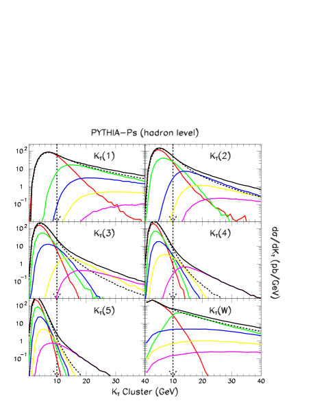
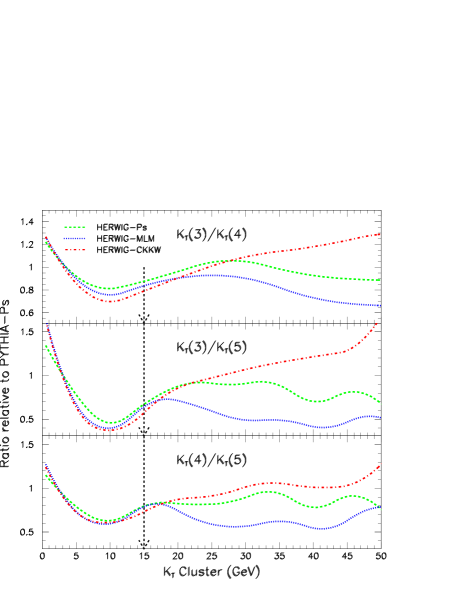
10.4 Discussion and Conclusions
We have compared three different procedures of matching ME predictions with PS’s using a methodology close to the CKKW algorithm suggested in [63, 76]: (1) a slightly expanded version of the CKKW procedure using HERWIG as the PS generator (but not limited in principal to HERWIG) and exploiting the freedom to choose scales and cut-offs; (2) a version of the CKKW procedure relying on pseudo-showers and matched closely to the scales and cut-offs of PYTHIA and HERWIG; and (3) a much simpler procedure based on the approach of M. Mangano. Results are summarized in Figs. 1 (a) and (b).
The HERWIG-CKKW procedure uses all of the elements of the original CKKW procedure, but expands upon them. Several choices of scale were investigated as starting points for the vetoed PS, and a wide range of prefactors were explored as arguments to the analytic NLL Sudakov form factor and . The variation of the results with these choices is shown in the figures. Optimized choices were settled upon based on the smoothness of distributions, the agreement with HERWIG where expected, and the apparent improvement over the default HERWIG predictions. While this appears to be a tuning, the final choices are easily justifiable. Since HERWIG is an angular-ordered shower, a variable such as -cluster values is well suited as a starting point for the HERWIG shower. Because of the details of the HERWIG shower, a prefactor of for the scale used in the Sudakov form factor is understandable, as well as a prefactor of for the scale used in evaluating . The results presented are better at the parton level than at the hadron level, which may require some tuning of the HERWIG hadronization model, and are less important at higher energies or when the cut-offs are larger.
The pseudo-shower procedure uses the Sudakov form factors of HERWIG and PYTHIA to numerically calculate the Sudakov suppression. Since the Sudakov form factor is a probability distribution for no parton emissions, the suppression factor can be determined by starting showers from different stages of the PS history and discarding those events with emissions above a given cut-off. Because of the nature of this approach, there is less tuning of parameters. To match the argument used in by default in HERWIG and PYTHIA, a different clustering scheme was used: clustering or LUCLUS-clustering. Final results at the hadron level are shown in the figures. In general, the hadron-level results are better than the parton-level ones. The use of LUCLUS over KTCLUS was driven by the kinematics of the PYTHIA shower. We have not checked whether KTCLUS works as well or better for the HERWIG results, and we leave this for future investigation. We should also investigate the advantages of using the exact clustering scheme of the individual generators: invariant mass and angular ordering for PYTHIA or just angular ordering for HERWIG. Also, since this work began, a new model of final-state showering was developed for PYTHIA which is exactly of the LUCLUS type. This should also be tested.
The MLM procedure is a logical extension of the procedure developed by M. Mangano for adding PS’s to +multijet events. It entails -clustering the parton-level events, adding a PS (with HERWIG in practice, but not limited to it), and rejecting those events where the PS generates a harder emission (in the -measure) than the original events. This approach yields a matching which is almost as good as the more complicated procedures based on the CKKW procedures explored in this work. The reason is not a pure numerical accident. The MLM procedure rejects events (equivalently, reweights them to zero weight) when the PS generates an emission harder than the lowest value of the given kinematic configuration. This is equivalent to the first step of the pseudo-shower procedure in the calculation of the Sudakov suppression when applied to the highest multiplicity ME. The remaining difference is in the treatment of the internal Sudakov form factors and the argument of . The agreement between the pseudo-shower and MLM procedures implies that the product of Sudakov form factors on internal lines with the factors of evaluated at the clustering scale is numerically equivalent to the product of factors evaluated at the hard scale. It is worth noting that, for the process at hand, , only two of the cluster values can be very close to the cut-off, and thus only two of the values can be very large. Also, at the matching scales considered in this study, GeV, with a factorization scale on the order of , , a fixed order expansion is of similar numerical reliability as the “all-orders” expansion of a resummation calculation. In fact, the resummation (PS) expansion is ideally suited for , whereas the fixed order expansion is best applied for .
Based on the study of these three procedures, we can make several statements on the reliability of predicting the shapes and rates of multijet processes at collider energies.
-
1.
The three matching procedures studied here can be recommended. They are robust to variation of the cut-off scale.
-
2.
The relative distributions in , for example, are reliably predicted.
-
3.
The variation in the relative distributions from the three procedures depends on the variable. For variables within the range of the ME’s calculated, the variation is 20%. For variables outside this range, which depend on the truncation of the ME calculation, the variation is larger 50%. Of course, it is important to study the experimental observables to correctly judge the senstivity to the cut-off and methodology of matching.
-
4.
More study is needed to determine the best method for treating the highest multiplicity ME contributions.
-
5.
The subject of matching is far from exhausted. The procedures presented here yield an improvement over previous matching prescriptions. However, these methodologies are an interpolation procedure.
Acknowledgments
This work was initiated at the Durham Monte Carlo workshop and has been performed in collaboration with P. Richardson. I thank T. Sjöstrand and J. Huston for discussion, encouragement and for asking the difficult questions. I also thank the Stephen Wolbers and the Fermilab Computing Division for access to the Fixed Target Computing Farms.
11 BOSON, DIRECT PHOTON AND TOP QUARK PRODUCTION: SOFT-GLUON CORRECTIONS 151515Contributed by: N. Kidonakis
11.1 Introduction
-boson, direct photon, and top quark production are all processes of considerable interest, useful in testing the Standard Model and searching for new physics. The hadroproduction cross sections for these processes have been calculated fully through next-to-leading order (NLO). Threshold corrections are known to be important in current hadron colliders and attempts have been made to calculate these soft-gluon corrections at next-to-next-to-leading order (NNLO) and beyond. Here I present results from the latest calculations.
In general, at each order in perturbation theory the partonic cross section for a hard-scattering process includes “plus” distributions with respect to a kinematical variable, denoted say as , that measures distances from partonic threshold. At -th order in the strong coupling (beyond the leading order) these distributions are of the type
| (8) |
where is a hard scale, such as a mass or transverse momentum, relevant to the process at hand. These logarithmic terms are the soft-gluon corrections and they arise from incomplete cancellations near partonic threshold between graphs with real emission and virtual graphs. This is due to the limited phase space available for real gluon emission near partonic threshold. These threshold corrections, calculated in the eikonal approximation, can be formally shown to exponentiate [79, 80, 81, 82] as a result of the factorization properties of the cross section. The logarithms with are denoted as leading (LL), with as next-to-leading (NLL), with as next-to-next-to-leading (NNLL), and with as next-to-next-to-next-to-leading (NNNLL). We note that the virtual corrections appear in terms. A unified approach and master formulas for the calculation of these corrections for any process at NNLO have recently been presented in Ref. [83]. For the processes discussed in the next three sections, the LL, NLL, and NNLL terms have been calculated fully. In the NNNLL terms we have not included some process-dependent two-loop contributions [83] which, however, we expect to be small.
11.2 Boson Production
The production of bosons in hadron colliders is a process of relevance in testing the Standard Model, calculating backgrounds to new physics such as associated Higgs boson production, and luminosity monitoring.
The calculation of the complete NLO cross section for hadroproduction at large transverse momentum was presented in Refs. [84, 85, 86]. The NLO results displayed an enhancement of the differential distributions in transverse momentum of the boson. The distribution falls rapidly with increasing , spanning five orders of magnitude in the 30 GeV 190 GeV region at the Tevatron.
-boson production at high transverse momentum receives corrections from the emission of soft gluons from the partons in the process. The resummation and NNLO-NNLL corrections were studied in Ref. [87]. More recently the NNLO-NNNLL corrections were studied in Ref. [88]. These threshold corrections further enhance the cross section and reduce the scale dependence [88].
For the hadronic production of a high- boson, with mass , the lowest-order partonic subprocesses are and . The partonic kinematical invariants in the process are , , , which satisfy at partonic threshold. Here is the invariant mass of the system recoiling against the boson and it parametrizes the inelasticity of the parton scattering. The partonic cross section includes distributions with respect to of the type .
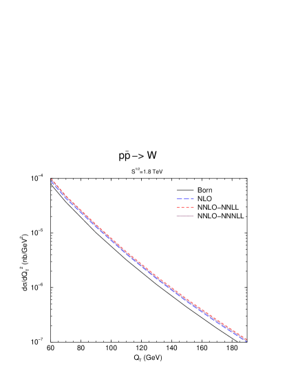
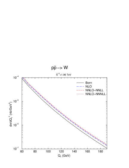
In Fig. 27 we plot the transverse momentum distribution, , for hadroproduction at the Tevatron Run I with TeV and Run II with TeV. We use the MRST2002 NNLO parton densities [89]. We set the factorization scale and the renormalization scale equal to . We focus on the high- region where the soft-gluon approximation holds well and the corrections are important. We see that the NLO corrections provide a significant enhancement of the Born cross section. The NNLO-NNLL corrections provide a further modest enhancement of the distribution. If we increase the accuracy by including the NNNLL contributions, which are negative, then we find that the NNLO-NNNLL cross section lies between the NLO and NNLO-NNLL results.
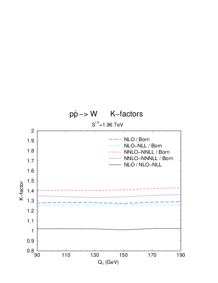
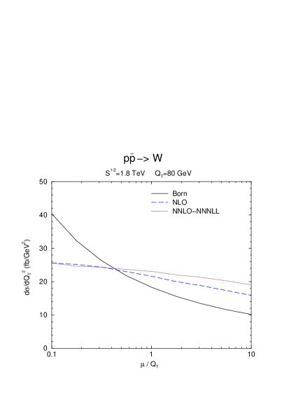
The -factors are shown at TeV in the left frame of Fig. 28. We see that the -factors are moderate, and nearly constant over the range shown even though the distributions themselves span two orders of magnitude in this range. It is also easy to see from the NLO/NLO-NLL curve that in the high region the soft-gluon approximation holds very well, as the NLO-NLL cross section is almost identical to the full NLO result.
The scale dependence of the differential cross section is shown on the right frame of Fig. 28 for GeV and TeV. We plot versus over two orders of magnitude: . We note the good stabilization of the cross section when the NLO corrections are included, and the further improvement when the NNLO-NNNLL corrections (which include all the soft and virtual NNLO scale-dependent terms) are added.
11.3 Direct Photon Production
Direct photon production is an important process for determinations of the gluon distribution function. The NLO cross section for direct photon production has been given in Refs. [90, 91, 92]. The role of higher-order soft-gluon corrections has also been addressed more recently. Threshold resummation and NNLO corrections for direct photon production have been presented in Refs. [93, 94].
At lowest order, the parton-parton scattering subprocesses are and . We define the Mandelstam invariants , , and , which satisfy at threshold. Note that the photon transverse momentum is . Here we calculate the cross section in the scheme. The soft corrections to the cross section appear in the form of plus distributions .
In order to show the effect of including the NNLO threshold terms, we start with a complete NLO calculation of the appropriate cross section using a program [95] which employs the phase-space slicing technique [96]. The original NLO calculation has been extended to include a complete NLO treatment of the bremsstrahlung contribution. The Set 2 fragmentation functions of [97] are used along with the CTEQ6M parton distribution functions [98]. In all cases the factorization and renormalization scales have been set equal to a common scale . Once the NLO results are obtained, the approximate NNLO contributions are then added to them.


In the left frame of Fig. 29 a comparison is made to data from the E-706 Collaboration [99]. The NNLO-NNNLL curve at is practically indistinguishable from the NLO except at high . However, the NNLO result is much higher than NLO, and as a result the scale dependence at NNLO is considerably reduced. The theoretical band lies below the data at the lower end of the range covered by the data. In the right frame of Fig. 29 the rapidity dependence is shown for the UA-6 proton proton data [100]. Again, the NNLO-NNNLL terms give a negligible contribution for the choice and the overall scale dependence is greatly reduced when the NNLO terms are added.
11.4 Top Quark Production
Recent calculations for top hadroproduction include NNLO soft-gluon corrections to the double differential cross section [101, 102, 103] from threshold resummation techniques. The latest calculation [103] includes NNNLL and some virtual terms (defined in Ref. [103]) at NNLO. When not all terms are known there is some difference between single-particle-inclusive (1PI) and pair-invariant-mass (PIM) kinematics. When NNNLL terms are included, the kinematics dependence of the cross section vanishes near threshold and is reduced away from it relative to NNLL accuracy. The factorization and renormalization scale dependence of the cross section is also greatly reduced.
We study the partonic process with and . In 1PI kinematics, a single top quark is identified, where is the identified top quark of mass and is the remaining final state that contains the . We define the kinematical invariants , , and . At threshold, , and the soft corrections appear as . In PIM kinematics, we have instead . At partonic threshold, , with the pair mass squared. The soft corrections appear as , with at threshold.

In Fig. 30 we present the NLO and approximate NNLO cross sections at TeV (left frame) and 1.96 TeV (right frame) for . We use the MRST2002 NNLO parton densities [89]. The NNLO results include the soft NNNLL and virtual terms in 1PI and PIM kinematics. We also show the average of the two kinematics results which may perhaps be closer to the full NNLO result.
In the left frame of Fig. 31 we show the scale dependence of the cross section, in the region , at TeV. The NLO cross section has a milder dependence on scale than the LO result. The NNLO cross section exhibits even less dependence on , approaching the independence of scale corresponding to a true physical cross section. The change in the NNLO cross section in the range , normally displayed as a measure of uncertainty from scale variation, is less than 3%. In the right frame of Fig. 31 we show the top quark transverse momentum distributions at TeV. At NNLO we observe an enhancement of the NLO distribution with no significant change in shape.
Finally we note that recently [104] NNLO threshold corrections were calculated for top quark production via flavor-changing neutral-current (FCNC) processes at the Tevatron and HERA colliders.

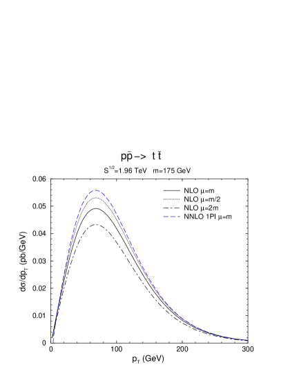
Acknowledgements
I would like to thank Jeff Owens, Agustin Sabio Vera, and Ramona Vogt for fruitful collaborations. The author’s research has been supported by a Marie Curie Fellowship of the European Community programme “Improving Human Research Potential” under contract number HPMF-CT-2001-01221.
12 EXTENDING THRESHOLD EXPONENTIATION BEYOND LOGARITHMS FOR DIS AND DRELL-YAN 161616Contributed by: T.O. Eynck, E. Laenen, L. Magnea
12.1 Introduction
Threshold resummation [105, 106] sums terms in cross sections that grow as a production threshold is approached. There is however empirical [107], theoretical [108, 105, 109, 110, 111, 112], as well as speculative [113] evidence of the fact that the formalism enabling threshold resummation could be extended to include classes of terms that are either constant or decrease upon the approach of threshold. The resummations of such terms, once put on a theoretically sound basis, would have significant phenomenological consequences, as shown in Ref. [107] for the case of Higgs production at hadron colliders.
The first evidence that the dominant non-logarithmic perturbative contributions could be exponentiated goes back to [108], where it was shown that the partonic Drell-Yan cross section in the DIS factorization scheme contains the ratio of the timelike to the spacelike Sudakov form factor: large perturbative contributions are left over in the exponentiated form of this ratio after the cancellation of IR divergences. This observation was made more precise in Ref. [105]. There, the resummation of threshold logarithms for the Drell-Yan process was proven to all logarithmic orders, making use of a procedure of refactorization: the Mellin transform of the cross section is expressed near threshold, approached by letting the Mellin variable grow very large, as a product of functions, each organizing a class of infrared and collinear enhancements; the refactorization is valid up to corrections which are suppressed by powers of at large , so that terms independent of can be treated by the same methods used to resum logarithms of .
It has also been clear for some time [110] that at least a subset of the terms enhanced by logarithms but suppressed by a power of can be resummed: in the scheme, for example, they arise from the exponentiation of the quark distribution. More recently, a factorization analysis of these terms was performed [111, 112], for the case of the longitudinal structure function in DIS, where however terms are the leading ones. It would be of considerable interest to extend this analysis to other processes. Since these logarithms arise at one loop from finite remainders of collinear singularities, which are suppressed by infrared power counting, it is conceivable that joint resummation [114] might provide a framework for an all-order treatment.
Here we report on recent work [115], where the results of Refs. [105, 109] were exploited to show that for processes which are electroweak at tree level (such as DIS and vector boson production through electroweak annihilation at colliders) the exponentation of -independent terms is in fact complete. The generalization of this result to processes with nontrivial color exchange is not straightforward, but it would of phenomenological interest for many processes to be studied at the LHC, including prompt photon, heavy quark and jet production.
12.2 Extended exponentiation for electroweak annihilation
Consider the Drell-Yan partonic cross section in the DIS scheme. The refactorization procedure described in Ref. [105] leads to the expression
| (9) |
The presence of the final-state jet function e.g. is direct consequence of dividing the unfactorized Drell-Yan cross section by the deep-inelastic structure function. A similar expression emerges in the scheme,
| (10) |
Notice the absence of , which does not occur in the density. Here is the quark form factor; , and are different quark distributions, with the same collinear singularities but different finite contributions: , in particular, is the distribution, consisting only of collinear poles; and are eikonal functions describing soft radiation at wide angles; finally is a jet function responsible for soft and collinear contributions from the final state DIS current jet. All functions exponentiate, and in each case real () and virtual () contributions have been separated. Finite virtual contributions in both cases can be expressed just in terms of the quark form factor. Note that although each function is divergent and thus depends on , the partonic cross sections are finite.
All functions involved in Eqs. (9) and (10) can be precisely defined in terms of quark fields and eikonal lines. Renormalization group analysis and explicit evaluation lead to expressions that have the familiar exponential form [106], with corrections involving -independent terms. For the DIS scheme one finds
Similarly, for the scheme one has the expressioon
| (12) | |||||
The functions and are given to order below in Eqs. (15) and (16). As is well-known [105, 106], the function is responsible for leading logarithms of to all orders. To achieve NLL accuracy one must compute it to two loops, obtaining
| (13) |
To NLL accuracy, one also needs the functions and to one loop, which are given by
| (14) |
The remaining ingredients, collecting -independent terms, are easily computed at one loop. For the DIS scheme one needs
| (15) |
For the scheme, one further needs
| (16) |
Notice finally that by taking the ratio of Eq. (12) and Eq. (12.2) one finds directly the (square of) the DIS structure function , factorized in the scheme, which can then be computed to the same accuracy without introducing other information. The ratio of form factors drops out from , as does the function [116], except for a contribution to the running between the physical scales and , which can be systematically reexpressed as a modification of the function .
All the functions appearing in Eq. (12.2) and Eq. (12) can be explicitly evaluated at two loops by matching with the complete two-loop calculation of Ref. [117]. An alternative, and often simpler method to determine the two-loop coefficients in these expressions uses equations derived from the fact that real and virtual contributions in the factorized expressions (16) and (10) are separately finite [115].
It is also important to keep in mind that the exponentiation of –independent terms does not have the predictive power of the standard resummation of threshold logarithms. In that case, typically, an entire tower of logarithms can be exactly predicted to all orders by performing just a low order calculation. Here, on the other hand, functions such as and receive new nontrivial contribution at each perturbative order. The exponentiation pattern is nonetheless nontrivial, and higher order terms predicted by the exponentiation can be considered representative of the size of the complete higher order correction [115].
13 JOINT RESUMMATION FOR TOP QUARK PRODUCTION 171717Contributed by: A. Banfi, E. Laenen
The formalism of joint resummation [118, 114] for hadronic cross sections of distributions singular at partonic threshold and at zero recoil has so far been applied to only a few processes. Recent studies involve processes that proceed at lowest order through a electroweak ( production [119]) or Yukawa interaction (Higgs production [53]). For these cases, the observables are the production cross sections at fixed mass and measured . Partonic threshold is then defined by , where is the partonic center of mass (cms) energy squared, and zero recoil by . At any finite order, the distributions take the form of plus-distributions and . Note that in these observables the latter distributions enter the physical cross sections, whereas the former are defined, after factorization, in the context of a perturbative analysis of the hard scattering.
In Ref. [120] the case of the prompt photon hadroproduction cross section at measured was analyzed, and a preliminary numerical study performed. In this case, a single-particle inclusive process proceeding through a reaction at lowest order, the identification of the recoil variable can only be made in the context of a refactorization analysis, just like the threshold variable . Through such an analysis, it is possible to identify a reduced hard scattering with cms energy squared and at transverse momentum with respect to the hadronic cms system. Note that this transverse momentum is invariant w.r.t. longitudinal boosts. In this way, the hard scattering need produce a photon with transverse momentum . It still remains to implement a procedure that consistently matches the joint resummed cross section to finite order calculations. In Refs. [114, 120] a simple cut-off was used in the integration over , with smaller that . For the prompt photon case, the hard scattering is singular at .
In this brief report we present a preliminary study of the application of joint resummation to another prominent single-particle inclusive cross section, the distribution of top quarks produced in hadronic collisions. Our motivation is to see what effect joint resummation has on a distribution in a TeV collider process that is nevertheless near threshold. Two key differences with the prompt photon case are (i) the heavy quark mass , preventing a singularity in the reduced hard scattering function when , and (ii) the possibility of multiple colored states for the produced top quark pair.
The jointly resummed expression for this observable can be written as
| (17) |
where
| (18) |
where the impact vector is Fourier conjugate to , and the variable is Laplace conjugate to the variable
| (19) |
where defines hadronic threshold. Furthermore
| (20) |
where . The exponentional function is given in Ref.[119] and are the Laplace moments of the lowest order heavy quark production matrix elements for either the or channel, the index labelling the color-state of the heavy quark pair.
In two figures we illustrate the effect of joint resummation over threshold resummation for the top quark ( GeV) spectrum for at Run II Tevatron, and only for the dominant channel. It produces the top quark pair at lowest order in an octet state. We use and toy densities .
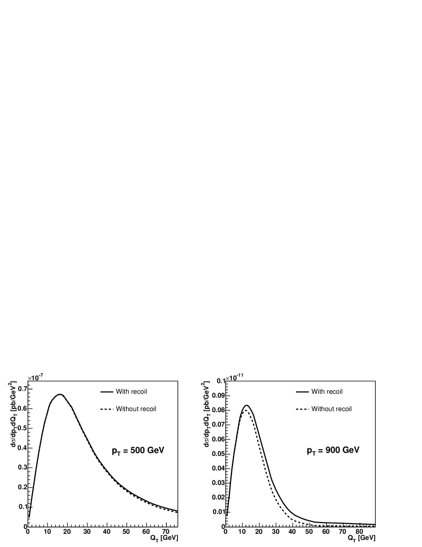
In Fig. 32 we exhibit the profile of Eq. (18) for two rather large values, in analogy to Fig. 1 in Ref.[120]. Note that these profiles are only of theoretical relevance, only their integral over can be measured. Recoil effects can be removed by neglecting in the last factor in Eq. (18). We observe a small enhancement over the threshold-resummed result, in particular at very large . Although not shown in the figure, there is in our case no divergence when approaches .
To keep the recoil soft with respect to the hard scale, we choose the cut-off . We can now show, in Fig. 33 the effect of joint resummation on the distribution, via Eq. (17). We observe only a small enhancement at very large values. The suppression at lower values is a consequence of the cut . A proper matching procedure should resolve this issue. Actually we note that this suppression is absent if we choose around 200 GeV.
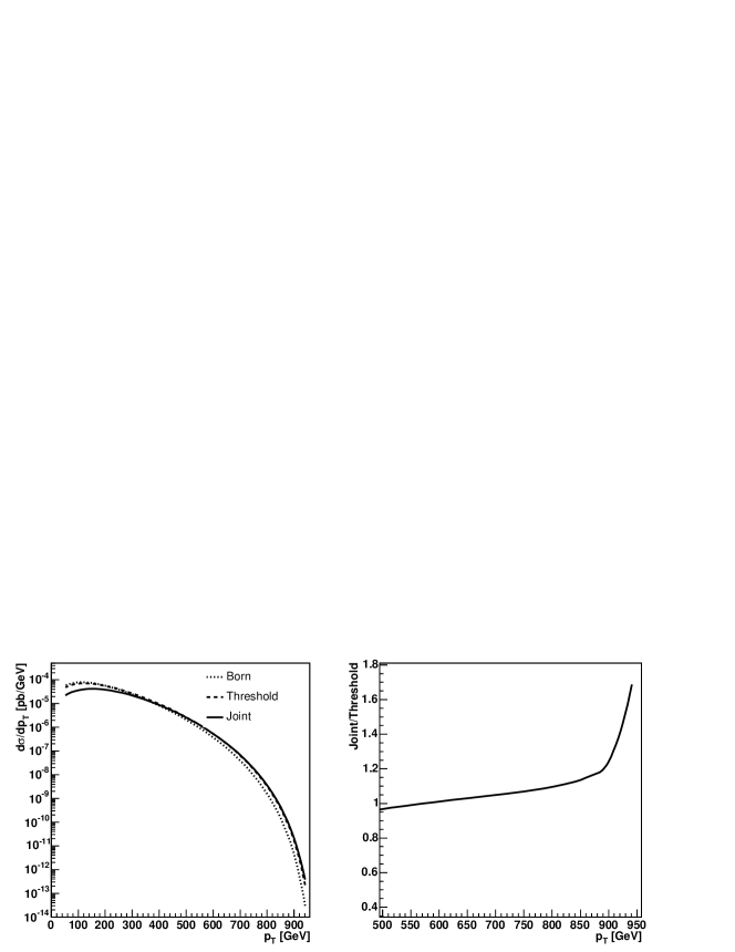
The enhancement at large is a consequence of what is effectively a smearing of the recoilless spectrum induced by perturbative radiation.
A more extenstive study including the channel and use of realistic parton distribution functions is forthcoming [121].
Acknowledgements
This work is supported by the Foundation for Fundamental Research of Matter (FOM) and the National Organization for Scientific Research (NWO).
14 A COMPARISON OF PREDICTIONS FOR SM HIGGS BOSON PRODUCTION AT THE LHC 181818Contributed by: C. Balazs, M. Grazzini, J. Huston, A. Kulesza, I. Puljak
14.1 Introduction
The dominant mechanism for the production of a SM Higgs boson at the LHC is gluon-gluon fusion through a heavy (top) quark loop. For this reason this channel has attracted a large amount of theoretical attention [122]. Recently, the total cross section has been calculated to NNLO in the strong coupling constant (i.e. at order ) [123, 124, 125, 126, 127] and also contributions from multiple soft gluon emission have been consistently included to NNLL accuracy [128]. In addition to the size of the total rate, a knowledge of the shape of the Higgs boson distribution is essential for any search and analysis strategies at the LHC. In particular, the distribution for the Higgs boson is expected to be harder than the one of its corresponding backgrounds. The Higgs boson distribution has been computed with LL parton shower Monte Carlos (HERWIG [70] and PYTHIA [7]), and through various resummed calculations. The latter techniques are the more powerful ones, but it is primarily the former that experimentalists at the LHC have to rely upon, because of their flexibility in allowing to test the effects of the various kinematic cuts which may optimize search strategies.
In the kinematic region , where most of the events are expected, large logarithmic corrections appear of the form that spoil the validity of the fixed order perturbative expansion. The distribution can be written as
| (21) |
The first term contains all logarithmically-enhanced contributions and requires their resummation to all orders. The second term is free from logarithmically-enhanced contributions and can be evaluated at fixed order in perturbation theory. The method to perform the all-order resummation is well known: to correctly take into account momentum conservation the resummation must be performed in the impact parameter () space [129, 130]. The large logarithmic contributions are exponentiated in the Sudakov form factor, which in the CSS [131] approach takes the form
| (22) |
where and . The and functions are free of large logarithmic corrections and can be computed as expansions in the strong coupling constant :
| (23) | |||||
| (24) |
The functions and control soft and flavour-conserving collinear radiation at scales . Purely soft radiation at a very low scales cancels out because the cross section is infrared safe and only purely collinear radiation up a scale remains, which is taken into account by the coefficients
| (25) |
Beyond NLL accuracy, to preserve the process independence of the resummation formula, an additional (process dependent) coefficient is needed [132], which accounts for hard virtual corrections and has an expansion
| (26) |
In the case of Higgs boson production through fusion, the relevant coefficients , and are known [133] and control the resummation up to NLL accuracy 191919There are two different classification schemes of the LL, NLL, NNLL, etc terms and their corresponding B contents. Here we use the most popular scheme. Another is discussed in Ref. [134].. The NNLL coefficients and are also known [135, 132]. The NNLL coefficient has been computed in Refs. [136, 137], whereas is not yet known exactly. In the following we assume that its value is the same that appears in threshold resummation [138].
14.2 Predictions for spectra and comparisons
In the 1999 Les Houches workshop, a comparison [139, 43] of the HERWIG and PYTHIA (2 versions) predictions for the Higgs boson distribution with those of a resummation program (ResBos [140, 52]) was carried out. This comparison was continued in the 2001 workshop and examined the impact of the coefficient [122]. In the meantime, a number of new theoretical predictions have become available, both from resummation and from the interface of NLO calculations with parton shower Monte Carlos. For these proceedings, we have carried out a comparison of most of the available predictions for the Higgs boson distribution at the LHC. We have used a Higgs boson mass of 125 GeV and either the MRST2001 or the CTEQ5M pdf’s. The difference between the two pdf’s for the production of a 125 GeV mass Higgs boson is of the order of a few percent. Before comparing the different predictions, we comment on the various approaches in turn.
Parton shower MC programs such as HERWIG, which implements angular ordering exactly, implicitly include the , and coefficients and thus correctly sum the LL and part of the NkLL contributions. However, in the most straightforward implementations, MC cannot correctly treat hard radiation. By contrast, the PYTHIA MC, which does not provide an exact implementation of angular ordering, has a hard matrix element correction 202020Very recently hard matrix element corrections for Higgs productions have been implemented in HERWIG as well [141].. Recently, an approach to match NLO calculations to parton showers generators, MC@NLO [55, 56], has been proposed, and applied, amongst the other, to Higgs production. This method joins the virtues of NLO parton level generators (correct treatment of hard radiation, exact NLO normalization) to the ones of MC. It thus can be compared to a resummed calculation at NLL+NLO accuracy.
As far as resummed calculations are concerned, we first consider two implementation of the CSS approach. The ResBos code includes the , and coefficients in the low- region and matches this to the NLO distribution at high . NNLO effects at high are approximately taken into account by scaling the second term in Eq. (21) with a K-factor. The matching is performed through a switching procedure whose uncertainty will be considered in the following. The calculation of Berger and Qiu [54] also performs a resummation in space and is accurate to NLL. The coefficient is included but the matching is still to NLO. Note that in both these approaches the integral of the spectrum is affected by higher-order contributions included in a non-systematic manner whose effect is not negligible for Higgs production.
The prediction by Bozzi, Catani, de Florian and Grazzini [51] (labeled Grazzini et al. in the following) is based on an implementation of the -space formalism described in [132, 51]. The calculation has the highest nominal accuracy since it matches NNLL resummation at small to the NNLO result at high [142]. This approach includes the coefficients and in approximated form. The main differences with respect to the standard CSS approach are the following. A unitarity constraint is imposed, such that the total cross section at the nominal (NNLO) accuracy is exactly recovered upon integration. A study of uncertainties from missing higher order contributions can be performed as it is normally done in fixed order calculations, that is, by varying renormalization and factorization scales around the central value, that is chosen to be .
Finally, we discuss the distribution of Ref. [53] (Kulesza et al.). This is obtained using a joint resummation formalism, by which both threshold and low- logarithmic contributions are resummed to all orders. This approach has been formally developed to NLL accuracy, but the NNLL coefficients and can also be incorporated. The matching is still performed to NLO. Even though a low mass Higgs boson at the LHC is produced with relatively low partons, threshold effects can still be significant due to the large color charge in the initial state as well as steep dependence of the gluon distribution functions at low . This leads to an increased sensitivity to Sudakov logarithms associated with partonic threshold for gluon-induced processes, as shown in Ref. [128].
It is known that the low- region is sensitive to non-perturbative effects. These are expected to be less important in the gluon channel due to the larger colour charge of the initial state [43]. Different treatments of non-perturbative effects are included in the ResBos, Berger et al. and Kulesza et al calculation, whereas Grazzini et al. prediction is purely perturbative.
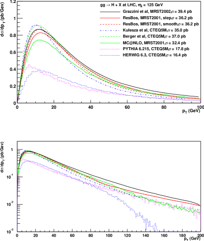
The absolute predictions for the cross sections are shown in Figure 34. All curves are obtained in the limit. HERWIG and PYTHIA cross sections are significantly smaller than the other predictions, their normalization being fixed to LO. In the high- region, the HERWIG prediction drops quickly due to the lack of hard matrix element corrections. PYTHIA, in contrast, features the hard matrix element corrections. We also note that PYTHIA prediction is significantly softer than all the other curves, and thus its overall shape is fairly different from all the other predictions.
The MC@NLO cross section, about 32.4 pb, is roughly twice that of the HERWIG and PYTHIA predictions, being fixed to the NLO total cross section.
Two predictions (step, smooth) are shown for ResBos which differ in the manner in which the matching at high is performed. Their difference can be considered as an estimate of the ambiguity in the switching procedure. The two curves correspond to the same total cross section of about 36.2 pb, which is about 8 % higher than the NLO cross section. This is the effect of the higher-order terms that enter the prediction for the total rate in the context of the CSS approach. A slightly softer curve is obtained by Berger and Qiu. The predicted cross section (37 pb) is close to that of ResBos.
The Grazzini et al. prediction has an integral of about 39.4 pb, which corresponds to the total cross section at NNLO. Contrary to what is done in Ref. [51], here the curve is obtained with MRST2002 NNLO partons and three-loop . The difference with the result obtained with MRST2001 NNLO PDFs is completely negligible.
Concerning the Kulesza et al curve, the subleading terms associated with low emission (i.e. in the limit opposite to partonic threshold) and of which only a subset is included in the joint resummation formalism, play an important role numerically. As a result, the total cross section turns out to be 35 pb, about lower than the pure threshold result, which is 39.4 pb [53].
We now want to examine in more detail the relative shapes of the predictions plotted in Figure. 34. In Figure. 35 all the predictions are normalized to the Grazzini et al. cross section of 39.4 pb.
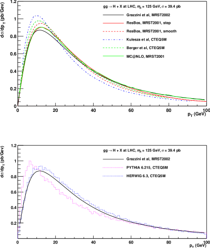
In the region of small and moderate (say, smaller than 100 GeV) all of the predictions are basically consistent with each other, with the notable exception of PYTHIA, which predicts a much softer spectrum. The curve of Kulesza et al. is also softer than the others.
For larger , HERWIG gives unreliable predictions, since the transverse momentum is generated solely by means of the parton shower, and therefore it lacks hard matrix element effects. The Grazzini et al. and ResBos curves are harder than MC@NLO for large . There are two reasons for this. Grazzini et al. implement the NNLO matrix elements exactly, corresponding to the emission of two real partons accompanying the Higgs in the final state [142]; ResBos mimics these contributions, by multiplying the NLO matrix elements by the K factor. MC@NLO, on the other hand, contains only NLO matrix elements (one real parton in the final state). Secondly, Grazzini et al. and ResBos choose the renormalization and factorization scales equal to , whereas in MC@NLO these scales are set equal to the transverse mass of the Higgs, . The difference is small at the level of total rates, but it is not negligible in the tail of the distribution.
14.3 Conclusions
Up to now, the ATLAS and CMS experiments have relied primarily on the predictions from HERWIG and PYTHIA in designing both their experiments as well as defining their search and analysis strategies. In the last few years, a number of tools for and predictions of the Higgs boson cross section at the LHC have become available, with the inclusion of beyond-the-leading-order effects at different level of accuracy. In the case of total rates, NNLO results have recently become available; their consistent inclusion in experimental analysis will allow to further decrease the estimated lower bound on the integrated luminosity to be collected for discovery.
In this contribution, we primarily focused on the predictions for the spectrum, comparing the results of Monte Carlos with those obtained with analytically-resummed calculations. In contrast to the situation in 1999, all of the predictions, with the exception of PYTHIA, result in the same general features, most notably in the position of the peak. However, differences do arise, because of different treatments of the higher orders. It is an interesting question beyond the scope of this review that of whether these differences are resolvable at the experimental level, which may lead to modify the strategy for searches. In order to answer this, studies including realistic experimental cuts must be performed with the newly available tools.
15 MATRIX-ELEMENT CORRECTIONS TO HIGGS IN HERWIG 212121Contributed by: G. Corcella, S. Moretti
15.1 The Higgs transverse momentum
In order to investigate Higgs boson production via Higgs (see Ref. [143]), one needs to account for multi-parton radiation for the sake of performing trustworthy phenomenological analyses [122, 144, 43]. Standard Monte Carlo (MC) algorithms [57, 70, 7] describe parton radiation in the soft and/or collinear approximation of the parton shower (PS), but can have regions of phase space, so-called ‘dead zones’, where no radiation is allowed. Here, one can however rely on higher-order tree-level results, as in this region the radiation is neither softly nor collinearly enhanced. Several methods have been recently suggested in order to match PS and fixed-order matrix elements (MEs) [75, 59], also including the virtual one-loop terms [55, 56, 145].
15.2 The HERWIG implementation
In this note, we briefly mention that the same strategy which has already been used to implement real ME corrections to annihilation into quark pairs [71], Deep Inelastic Scattering (DIS) [72], top quark decay [73] and vector boson hadro-production [74] has now also been adopted for the case of Higgs hadro-production via gluon-gluon fusion, in the context of the HERWIG event generator [57, 70]. That is, the dead zone is here populated by using the exact next-to-leading order (NLO) tree-level ME result and the PS in the already-populated region is corrected using the exact amplitude any time an emission is capable of being the hardest so far.
15.3 Numerical results and comparisons
The MEs squared for the real corrections to that we have used can be found in [146], where top mass effects are fully included. The real NLO corrections to are instead rather straightforward: the formulae we used can be read from Eq. (3.62) of [147] with appropriate Yukawa couplings and crossing. In the new HERWIG default version, in line with [74], ME corrections use the Higgs transverse mass as the scale for and for the Parton Distribution Functions (PDFs) while the contributions use . We shall also assume that the intrinsic transverse momentum of the initial-state partons is equal to , the HERWIG default value.


By adopting the HERWIG defaults, we first consider Higgs production at the Tevatron and the LHC within the MC itself, by plotting the distribution with (solid histogram) and without (dotted) ME corrections: see Fig. 36. Beyond the ME-corrected version allows for many more events. In fact, one can prove that, within the standard algorithm, is constrained to be . At small the prediction which includes ME corrections displays a suppression. By default, after the latter are put in place, the total normalization still equals the LO rates. Hence, it is obvious that the enhancement at large implies a reduction of the number of events which are generated at small values.
In Fig. 37 (left plot) we present the improved HERWIG spectrum (solid) for the LHC, along with the result obtained running the so-called ‘ + jets’ process (dotted), where the hard process is always one of the corrections to . In order to perform such a comparison, we have turned the hard process off, as ‘ + jets’ in HERWIG does not currently implement the corrections to quark-antiquark annihilation. Furthermore, we have chosen GeV for the ‘ + jets’ generation. As expected, at small the two predictions are fairly different but at large transverse momentum they agree well.
In Fig. 37 (centre plot) we compare the new HERWIG version with the resummed calculation of Ref. [51]. For the sake of comparison with HERWIG, which includes leading logarithms and only some subleading terms, we use the results of [51] in the NLL approximation (rather than the default NNLL one), matched to the NLO prediction. In order for such a comparison to be trustworthy, we have to make parameter choices similar to [51]: namely, we adopt a top quark with infinite mass in the loop and GeV, with and PDFs (both from HERWIG defaults) evaluated at . While the normalization (LO in HERWIG, NLO in Ref. [51]) and the small- behaviour of the two curves are clearly different, the large transverse momentum predictions are in good agreement, as in both approaches it is the real NLO ME that dominates the event generation at large .
Finally, in Fig. 37 (right plot), we compare the results of standard HERWIG after ME corrections with the MC@NLO event generator (version 2.2) of Ref. [148], the latter implementing both real and virtual corrections to the hard-scattering process, in such a way that predicted observables (including normalization) are correct to NLO accuracy. As version 2.2 of the MC@NLO includes only the corrections to Higgs production in the gluon-fusion channel, we again have turned the quark-annihilation process off in our routines. As observed in the comparison with the resummed calculation, the two spectra differ in normalization and at small , but agree in the large-transverse-momentum region.
15.4 Conclusions
Between the described implementation and the one available within the MC@NLO option, we believe that HERWIG is presently a reliable event generator for (direct) Higgs production from parton fusion at hadron colliders both at small and large transverse momentum. In fact, all currently available ME corrections will play an important role to perform any analysis on Higgs searches at present and future colliders. In particular, the option described here may be the most convenient choice for when the phase space is limited to transverse momentum values such that .
Acknowledgements
SM would like to thank the 2003 Les Houches workshop organisers for their kind invitation and the Royal Society (London, UK) for financial support.
16 CAESAR: AUTOMATING FINAL-STATE RESUMMATIONS 222222Contributed by: A. Banfi, G.P. Salam, G. Zanderighi
Event shapes and jet resolution parameters (final-state ‘observables’) measure the extent to which the energy-flow of the final state departs from that of a Born event. Their study has been fundamental for measurements of the strong coupling [149, 150] as well as the QCD colour factors [151]; final states also provide valuable information on the yet poorly understood transition from parton to hadron level (see [152] for a recent review). In the region where an observable’s value is small, one should resum logarithmically enhanced contributions that arise at all orders in the perturbative series. For a number of observables such a resummation has been carried out manually at next-to-leading logarithmic (NLL) accuracy [153]. But achieving NLL accuracy requires a detailed analysis of the observable’s properties, and is often technically involved. We have instead recently proposed [154] a new approach based on a general NLL resummed master formula valid for a large class of final-state observables (which includes many of the final-state observables for which a NLL resummation already exists). We have also formulated the formal requirements that an observable should satisfy so as to be within the scope of the master formula.
To illustrate these requirements we consider a Born event consisting of hard partons or ‘legs’. For an observable (a function of all final-state momenta) to be resummed in the -jet limit it should:
-
1.
vanish smoothly after addition of an extra soft particle collinear to any leg , with the following behaviour:
(27) Here is a hard scale of the problem; represents the Born (hard) momenta after recoil from the emission, which is defined in terms of its transverse momentum and rapidity with respect to leg , and where relevant, by an azimuthal angle relative to a Born event plane.
-
2.
be recursively infrared and collinear (rIRC) safe: meaning roughly that, given an ensemble of emissions, the addition of a relatively much softer or more collinear emission does not significantly alter the value of the observable, no matter how soft and/or collinear the other emissions are. This condition is necessary to ensure exponentiation of leading logarithms, and is not satisfied for example by the JADE algorithm three-jet resolution parameter [155].
-
3.
be continuously global, meaning that the observable is sensitive to emissions in the whole of the phase space (‘global’) in a continuous way, the formal requirement being and ( being defined with respect to the nearest leg). For non-continuously-global observables one must account for non-global logarithms (known only for large ) [156]. Their evaluation for a general observable would necessitate a (quite non-trivial) determination of the phase-space boundaries associated with the observable.
Given the above conditions, the NLL resummation for the observable’s distribution (the probability that the observable’s value is less than ) for a fixed Born configuration is given by the ‘master’ formula [154]:
| (28) |
The function is a Sudakov exponent that contains all leading (double) logarithms and all NLL (single-log) terms that can be taken into account by exponentiating the contribution to from a single emission. This function depends parametrically on and on the azimuthal average ; its full expression is reported in [154]. Multiple emission effects, for example the fact that even if all , one might nevertheless have , are accounted for by the NLL function , which can be computed via a Monte Carlo procedure [157].
The advantage of having introduced a master formula is that the resummation of the observable can be performed entirely automatically. The master formula and applicability conditions are encoded in a computer program (CAESAR, Computer Automated Expert Semi-Analytical Resummer), which given only the observable’s definition in the form of a computer routine, returns the observable’s distribution at NLL accuracy (where possible).
As an example we present explicit results for the specific case of the (global) transverse thrust in hadronic dijet production, defined as
| (29) |
where the sums run over all particles in the final state, the are the particle transverse momenta (with respect to the beam direction) and is a unit transverse vector. The program, probing the observable with randomly chosen soft and collinear emissions, is able to verify that the applicability conditions hold and to determine the parameters , as well as the function . It then applies the Monte Carlo procedure introduced in [157] to compute the function . The results from this analysis are then plugged into the master formula (28) to compute at NLL accuracy. The resulting differential distribution (integrated over a range of Born configurations, with the cuts given below) is shown in figure 38 for the most relevant partonic subprocesses at the Tevatron run II c.o.m. energy TeV. We select events with two outgoing jets with GeV and , use the CTEQ6M parton density set [98], corresponding to , and set both the renormalisation and factorisation scale at the Born partonic c.o.m. energy. The curves in figure 38 show a degree of separation between the various partonic channels — this information could perhaps be exploited in fits of parton distributions.
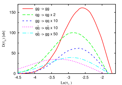
To conclude we remark that since the only input to CAESAR is a computer subroutine for an observable, it offers for the first time the possibility for non-experts to easily obtain rigorous NLL resummed predictions. Work remains to be done both to release the first version of CEASAR and to implement automated matching of NLL resummation with fixed order results. In particular, addressing this last issue will open the way for a vast amount of phenomenological analyses.
17 COMBINED EFFECT OF QCD RESUMMATION AND QED RADIATIVE CORRECTION TO BOSON MASS MEASUREMENT AT THE LHC 232323Contributed by: Q.-H. Cao, C.-P. Yuan
17.1 Introduction
As a fundamental parameter of the Standard Model (SM), the mass of the -boson () is of particular importance. Aside from being an important test of the SM itself, a precision measurement of , together with an improved measurement of top quark mass (), provides severe indirect bounds on the mass of Higgs boson (). With a precision of 15 MeV for [158] and 2 GeV for at the LHC [159], in the SM can be predicted with an uncertainty of about 30% [158]. Comparison of these indirect constraints on with the results from direct Higgs boson searches, at the LEP2, the Tevatron and the CERN Large Hadron Collider (LHC), will be an important test of the SM. In order to have a precision measurement of , the theoretical uncertainties, dominantly coming from the transverse momentum of the -boson (), the uncertainty in parton distribution function (PDF) and the electroweak (EW) radiative corrections to the boson decay, must be controlled to a better accuracy [160, 158].
At the LHC, most bosons are produced in the small transverse momentum region. When is much smaller than , every soft-gluon emission will induce a large logarithmic contribution to the distribution so that an order-by-order perturbative calculation in the theory of Quantum chromodynamics (QCD) cannot accurately describe the spectrum and the contribution from multiple soft-gluon emission, which contributes to all orders in the expansion of the strong coupling constant , needs to be summed to all orders. It has been shown that by applying a renormalization group analysis, the multiple soft-gluon radiation effects can be resummed to all orders to predict the distribution which agrees with experimental data [161, 140]. RESBOS, a Monte Carlo (MC) program [140] resumming the initial-state soft-gluon radiations of the hadronically produced lepton pairs through EW vector boson production and decay at hadron colliders , has been used by the CDF and DØ Collaborations at the Tevatron to compare with their data in order to determine . However, RESBOS does not include any higher order EW corrections to describe the vector boson decay. The EW radiative correction, in particular the final-state QED correction, is crucial for precision measurement of boson mass at the Tevatron, because photon emission from the final-state charged lepton can significantly modify the lepton momentum which is used in the determination of . In the CDF Run Ib mass measurement, the mass shifts due to radiative effects were estimated to be MeV and MeV for the electron and muon channels, respectively [162]. The full next-to-leading order (NLO) EW corrections have been calculated [163, 164] and resulted in WGRAD [164], a MC program for calculating EW radiative corrections to the process . However, WGRAD does not include the dominant correction originated from the initial-state multiple soft-gluon emission. The inclusion of both the initial-state QCD and final-state QED corrections into a parton level MC program is urgently required in order to reduce the theoretical uncertainties in interpreting the experimental data at the Tevatron. It was shown in Refs. [163, 164] that at the NLO, the EW radiative correction in is dominated by the final-state QED (FQED) correction. Hence, in this paper we present a consistent calculation which includes both the initial-state multiple soft-gluon QCD resummation and the final-state NLO QED corrections, and develop an upgraded version of the RESBOS program, called RESBOS-A 242424A Fortran code that implements the theoretical calculation is presented in this work., to simulate the signal events. Here, we only present the phenomenological impacts on a few experimental observables, the transverse mass of boson () and the transverse momentum of charged lepton (), that are most sensitive to the measurement of . We focus our attention on the electron only, though our analysis procedure also applies to the muon. The detailed formula, the SM inputting parameters and the kinematics cuts are given in Ref. [165].
17.2 Precision Measurement of W Mass
In Fig. 39, we show various theory predictions on the distribution. The legend of the figure is defined as follows:
-
LO : including only the Born level initial-state contribution,
-
RES : including the initial-state multiple soft-gluon corrections via QCD resummation,
-
LO QED : including only the Born level final-state contribution,
-
NLO QED : including the final-state NLO QED corrections.
For example, the solid curve (labelled as RES+NLO QED) in Fig. 39(a) is the prediction from our combined calculation, given by Eqs. (1) and (2) of Ref [165].
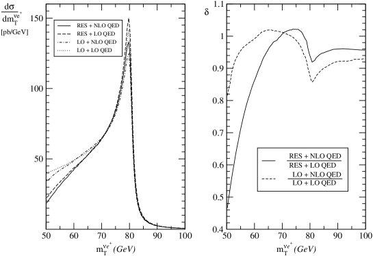
As shown in Fig. 39(a), compared to the lowest order cross section (dotted curve), the initial state QCD resummation effects (dashed curve) increase the cross section at the peak of the distribution by about , and the final state NLO QED corrections (dot-dashed curve) decrease it by about , while the combined contributions (solid curve) of the QCD resummation and FQED corrections reduce it by . In addition to the change in magnitude, the line-shape of the distribution is significantly modified by the effects of QCD resummation and FQED corrections. To illustrate this point, we plot the ratio of the (RES+NLO QED) differential cross sections to the LO ones as the solid curve in Fig. 39(b). The dashed curve is for the ratio of (LO+NLO QED) to LO. As shown in the figure, the QCD resummation effect dominates the shape of distribution for , while the FQED correction reaches its maximal effect around the Jacobian peak (). Hence, both corrections must be included to accurately predict the distribution of around the Jacobian region to determine . We note that after including the effect due to the finite resolution of the detector (for identifying an isolated electron or muon), the size of the FQED correction is largely reduced [163, 164].
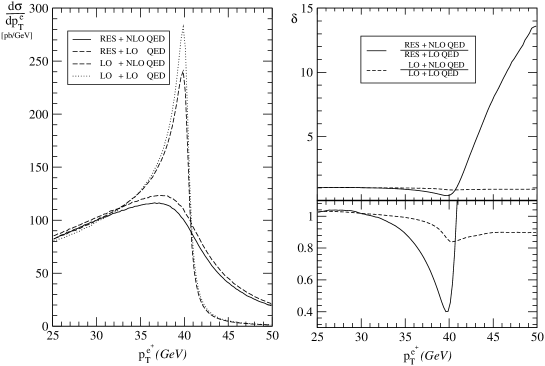
Although the distribution is an optimal observable for determining at the LHC with a low luminosity, it requires an accurate measurement of the missing transverse momentum direction which becomes more difficult to control with a high luminosity option (when multiple scattering becomes important). On the other hand, the transverse momentum of the decay charged lepton () is less sensitive to the detector resolution, so that it can be used to measure and provide important cross-check on the result derived from the distribution, for they have different systematic uncertainties. Another important feature of this observable is that distribution is more sensitive to the transverse momentum of boson. Hence, the QCD soft-gluon resummation effects, the major source of , must be included to reduce the theoretical uncertainty of this method. In Fig. 40(a), we show the distributions predicted by various theory calculations, and in Fig. 40(b), the ratios of the higher order to lowest order cross sections as a function of . The lowest order distribution (dotted curve) shows a clear and sharp Jacobian peak at , and the distribution with the NLO final-state QED correction (dot-dashed curve) also exhibits the similar Jacobian peak with the peak magnitude reduced by about . But the clear and sharp Jacobian peak of the lowest order and NLO FQED distributions (in which ) are strongly smeared by the finite transverse momentum of the boson induced by multiple soft-gluon radiation, as clearly demonstrated by the QCD resummation distribution (dashed curve) and the combined contributions of the QCD resummation and FQED corrections (solid curve). Similar to the distribution, the QCD resummation effect dominates the whole range, while the FQED correction reaches it maximum around the Jacobian peak (half of ). The combined contribution of the QCD resummation and FQED corrections reaches the order of near the Jacobian peak. Hence, these lead us to conclude that the QCD resummation effects are crucial in the measurement of from fitting the Jacobian kinematical edge of the distribution.
As shown in Ref. [140], the effect from the initial state QCD gluon resummation to the W transverse mass distribution is dominated by the perturbative Sudkov contribution and is not very sensitive to the non-perturbative parameters ( and ) of the CSS resummation formalism. On the other hand, as shown in Fig. 39, the final state QED correction can largely modify the W transverse mass distribution, though a definite conclusion can only be drawn after including the effect of detector resolution.
In our calculation we have included the contributions from the final state QED correction together with the initial state QCD resummation to predict the production and decay of W bosons produced at the LHC. Since the exact matrix elements have been used in the calculation, the spin correlations among the initial state partons and final state leptons are correctly implemented. Hence, the kinematic distributions of the final state leptons, and the corresponding experimental observables, can be reliably predicted.
In order to study the impact of the presented calculation to the determination of the boson mass, the effect due to the finite resolution of the detector should be included, which will be presented elsewhere.
We thank P. Nadolsky and J.W. Qiu for helpful discussions. This work was supported in part by NSF under grand No. PHY-0244919 and PHY-0100677.
18 RESUMMATION FOR THE TEVATRON AND LHC ELECTROWEAK BOSON PRODUCTION AT SMALL 252525Contributed by: S. Berge, P. Nadolsky, F. Olness, C.-P. Yuan
In the production of electroweak bosons, precise knowledge of the transverse mass and transverse momentum provides detailed information about the production process, including the mass of the boson and associated radiative corrections. At the Tevatron, distributions of bosons offer insight into soft gluon radiation, and this information is then used for precision extraction of the boson mass. At the LHC, good knowledge of the transverse distribution of Higgs bosons will be needed to efficiently separate Higgs boson candidates from the large QCD background. Accurate predictions for the small- region are obtained via resummation of large logarithms arising from unsuppressed soft and collinear radiation in higher orders of perturbation theory.
As we move from the 2 TeV Tevatron to the 14 TeV LHC, typical values of partonic momentum fractions for producing , , and bosons become smaller, thus enhancing terms in higher orders of . It is not entirely known how these terms (not included in a fixed-order cross section or conventional resummation) will affect , , and production at the LHC energies, in part because no Drell-Yan data is available yet in the relevant region of of a few or less.
Studies [166, 167] in the crossed channel of semi-inclusive deep-inelastic scattering (SIDIS) suggest that hadronic distributions at small cannot be straightforwardly described within the Collins-Soper-Sterman (CSS) resummation framework [131], if the nonperturbative Sudakov function behaves like its large- counterpart from the Drell-Yan process. A distribution in SIDIS at is substantially broader than the conventional CSS prediction. The broadening effect can be modeled by including an extra -dependent term in the Sudakov exponent. To describe the data, the extra term must grow quickly as . It noticeably contributes to the resummed form factor at intermediate impact parameters (), which hints at its origin from perturbative physics. A possible interpretation of this term is that it mimics higher-order contributions of the form , which are not included in the resummed cross section. Due to the two-scale nature of the resummation problem, the non-resummed terms may affect the distribution even when they leave no discernible trace in inclusive DIS structure functions. The DIS structure functions depend on one hard scale (of order ), while the CSS resummation formula (cf. Eq. (30)) also includes contributions from large impact parameters (small momentum scales). As becomes large, the series in the CSS formula may begin to diverge at a larger value of than the series in the inclusive structure functions. For this reason, transition to -unordered (BFKL-like [168, 169]) physics may happen at larger in distributions than in inclusive (one-scale) observables.
The broadening discussed above was observed in semi-inclusive DIS processes. In this study, we explore its possible implications for the (crossed) Drell-Yan process. We begin by examining the resummed transverse momentum distribution for the Drell-Yan process [131], following notations from Ref. [170]:
| (30) |
Here , the integral is the Fourier transform of a resummed form factor given in impact parameter () space, and is a regular (finite at ) part of the fixed-order cross section. In the small- limit, the form factor is given by a product of a perturbative Sudakov exponent and generalized parton distributions :
| (31) |
At moderately small , where the representation (31) for holds, we write these generalized parton distributions in the form
| (32) |
where are coefficient functions, are conventional parton distributions, and is a commonly appearing constant factor.
The term in will provide an additional broadening, with an dependence specified by . For example, it may approximate -dependent higher-order contributions that are not included in the finite-order expression for . We parametrize in the following functional form:
| (33) |
such that for , and for . This parameterization ensures that the formalism reduces to the usual CSS form for large () and introduces an additional source of broadening (growing as ) at small (). The parameter determines the magnitude of the broadening for a given , while specifies the value of below which the broadening effects become important. In principle, and may depend on the hard scale ; in this first study, we neglect this dependence. Based on the observed dependence at in SIDIS energy flow data [167], we choose and as a representative choice for our plots.
As , the additional broadening term in Eq. (32) affects the form factor both at perturbative () and nonperturbative () impact parameters. In addition, the resummed cross section contains conventional non-perturbative contributions from power corrections, which become important at large impact parameters (). We introduce these corrections by replacing the impact parameter in functions and with a variable [131] and including a nonperturbative Sudakov exponent . The function is parametrized by a 3-parameter Gaussian form from a recent global fit to low-energy Drell-Yan and Tevatron Run-1 data [170]. Combining all the terms, we have:
| (34) | |||||
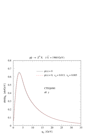
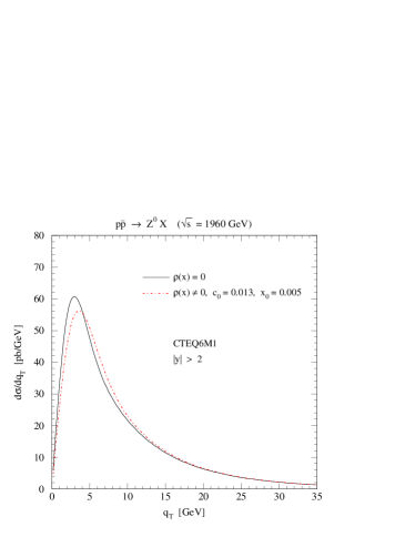
(a) (b)
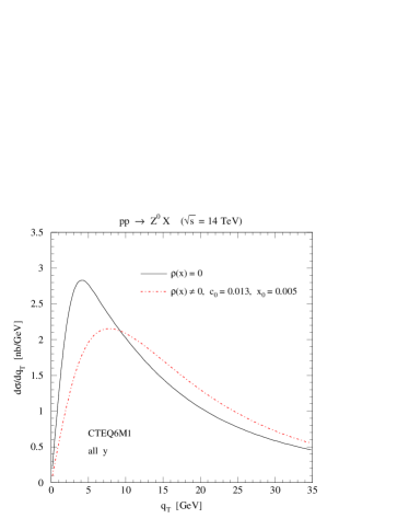
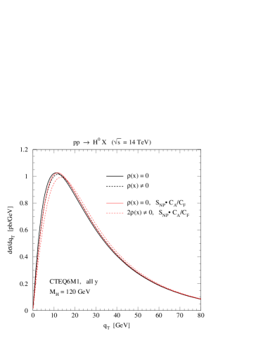
(a) (b)
Figs. 41 and 42 show the comparison of the resummed cross section (34) with the additional broadening term () to the resummed cross section without such a term (). We consider cross sections for the production of and bosons, calculated according to the procedures in Refs. [140] and [52], respectively. The numerical calculation was realized using the programs Legacy and ResBos [170, 140], and with the CTEQ6M1 parton distribution functions [171]. The perturbative Sudakov factor was included up to , and the functions up to . The relevant perturbative coefficients can be found in Refs. [131, 172, 173, 133, 174, 175, 136, 132].
Fig. 41(a) shows the differential distribution for boson production in the Tevatron Run-2, integrated over the rapidity of the bosons. We observe that the distribution (34) with the additional small- term (the dashed curve) essentially coincides with the standard CSS distribution (the solid curve). When is integrated over the full range, both resummed cross sections are dominated by contributions from , where the additional broadening (given by the function ) is negligible. For this reason, the Tevatron distributions that are inclusive in (e.g., the Run-1 boson data) will not be able to distinguish the small- broadening effects from uncertainties in the nonperturbative Sudakov function .
In contrast, the small- broadening does lead to observable differences in the distributions in the forward rapidity region, where one of the initial-state partons carries a smaller momentum fraction than in the central region. Fig. 41(b) shows the cross section for bosons satisfying . The peak of the curve with is lower and shifted toward higher . While this difference was not large enough to be observed in the Tevatron Run-1, it seems to be measurable in the Run-2 given the improved acceptance and higher luminosity of the upgraded Tevatron collider. The small- broadening is more pronounced in boson production due to the smaller mass of the boson.
We now turn to the LHC, where the small- broadening may be observed in the whole rapidity range due to the increased center-of-mass energy. Fig. 42(a) displays the distribution for production with and without the small- terms. Here, the difference is striking even if is integrated out. Effects of a similar magnitude are present in boson production, and they are further enhanced in the forward regions.
The small- broadening is less spectacular, but visible, in the production of light Standard Model Higgs bosons via the effective vertex in the limit of a heavy top quark mass. Fig. 42(b) displays the resummed cross sections for production of Higgs bosons with a mass GeV for several choices of and the broadening term. We first compare cross sections for and (thick lines), where the functions and are taken to be the same as in boson production. The difference between the two cross sections is not large, due to a harder spectrum in the Higgs boson case. The peaking in the -dominated distribution occurs at GeV, i.e., beyond the region where the function play its dominant role. This is different from the -dominated distribution, where the peak is located at GeV and is strongly affected by . Hence, for the same function as in the boson case, the difference between the curves with and without is minimal.
The harder spectrum in the Higgs boson case is induced by a larger leading-logarithm coefficient () in channels, as compared to the leading-logarithm coefficient in channels. This suggests that the -dependent part (and possibly other terms) of the nonperturbative Sudakov function in Higgs boson production is also multiplied by a larger color factor than in the Drell-Yan process. We estimate this effect by multiplying by the ratio of the leading color factors in Higgs and boson production processes, (the thin solid line). The resulting change turns out to be small because of the reduced sensitivity of the Higgs boson cross section to nonperturbative contributions.
The terms may be enhanced in the case of the Higgs bosons as well, due to the direct coupling of the Higgs bosons to gluon ladders. At present, we do not have a reliable estimate of the small- broadening in gluon-dominated channels. However, this broadening would have to be quite large to affect of 10-20 GeV or more, i.e., in the region where selection cuts on of the Higgs boson candidates will be imposed. For example, increasing the function by a factor of two as compared to the boson case would lead to a distribution shown by the thin dashed line. While at GeV this effect is relatively small as compared to other theory uncertainties (e.g., higher-order corrections), it may affect precision calculations of distributions needed to separate the Higgs boson signal from the background in the mode.
Additional constraints on the small- behavior of the resummed cross sections in the channel could be obtained from examination of photon pair production away from the Higgs signal region. As the mass of the photon pair decreases, production in the gluon fusion channel via a quark box diagram becomes increasingly important. For instance, the subprocess contributes up to 40% of the total cross section at GeV [176]. By comparing distributions in and in the same region of , one may be able to separate the and components of the resummed cross section and learn about the dependence in the channel.
To summarize, we argue that a measurement of transverse momentum distributions of forward bosons at the Tevatron will provide important clues about the physics of QCD factorization and possibly discover broadening of distributions associated with the transition to small- hadronic dynamics. Based upon the analysis of broadening effects observed in semi-inclusive DIS, we have estimated similar effects in the (crossed) processes of electroweak boson production at hadron-hadron colliders. While the estimated impact on the Higgs boson cross section at high was found to be minimal, much larger effects may occur in and boson production in the forward region at the Tevatron Run-2, and at the LHC throughout the full rapidity range. If present, the small- broadening will have to be taken into consideration in precision studies of electroweak boson production. Additionally, its observation will provide insights about the transition to -unordered (BFKL-like) dynamics in multi-scale distributions at hadron-hadron colliders.
Acknowledgments
We thank C. R. Schmidt for valuable discussions. This work was supported by the U.S. Department of Energy under grant DE-FG03-95ER40908, the National Science Foundation under grant PHY-0244919, and the Lightner-Sams Foundation.
19 THE HIGH ENERGY LIMIT OF QCD AND THE BFKL EQUATION 262626Contributed by: J. R. Andersen, V. Del Duca,A. De Roeck, A. Sabio Vera
The Balitsky–Fadin–Kuraev–Lipatov (BFKL) [177, 178, 168, 179, 169, 180] formalism resums a class of large logarithms dominant in the Regge limit of scattering amplitudes, where the center of mass energy is large and the momentum transfer fixed. The cross–section for a general process within this approach in the high energy limit can be written in the factorised form
| (35) |
where are the impact factors characteristic of the particular scattering process and is the gluon Green’s function describing the interaction between two Reggeised gluons exchanged in the –channel with transverse momenta . When these two transverse momenta are large and of similar magnitude the Regge scale is chosen as the scaling factor in the large logarithms. The implicit –dependence of the NLL impact factors cancels that of the BFKL gluon Green’s function so as to render the cross section independent of to this accuracy. In the leading logarithmic (LL) approximation terms of the form are resummed, while in the next–to–leading logarithmic (NLL) approximation [181, 182] contributions of the type are also taken into account.
The gluon Green’s function is obtained as the solution of an integral equation, the so called BFKL equation, where radiative corrections enter through its kernel. At LL it is possible to construct the complete eigenfunctions of this kernel and, consequently, calculate the solution analytically. At NLL this is only possible up to terms directly related to the running of the strong coupling; this means that solving the BFKL equation at NLL with the full kernel is a very challenging problem. Good progress has been made in the last few years in this field: Studies of the stability of the perturbative expansion were performed in [183, 184, 185, 186, 187, 188, 189, 190, 191, 192, 193] and of running coupling effects in [194, 195, 196, 197, 198, 199, 200, 201, 202, 203]. Among the most recent work studying the gluon Green’s function an analysis based on a new renormalisation group improved small x resummation scheme was proposed in Ref. [204]; in Ref. [205] an anomalous dimension including running couplings effects was constructed; and in Ref. [206, 207] the Green’s function and gluon splitting function were studied including a particular resummation scheme.
In this contribution we report on the progress made in the last year to solve the NLL BFKL equation exactly in a novel way: Using the numerical implementation of an iterative solution presented in Ref. [208, 209] found by explicitly separating the virtual contributions to the kernel from the real emissions in transverse momentum space. This is achieved by introducing a phase space slicing parameter in dimensional regularisation. How to obtain this solution, which includes the angular correlations present in the kernel and the running coupling effects, is presented in the next section.
19.1 A novel solution to the NLL BFKL equation 272727Contributing authors: J. R. Andersen, A. Sabio Vera
It is convenient to introduce the Mellin transform in space
| (36) |
in order to write the NLL BFKL equation in dimensional regularisation as
| (37) |
with the kernel depending on the gluon Regge trajectory, which includes the virtual contributions, and a real emission component [181]. The delta function in the driving term of the integral equation corresponds to the limit of two gluon exchange.
The phase space slicing parameter, , is introduced through the approximation
| (38) | |||||
which is a valid one for small values of the infrared parameter . With this separation it is possible to show that the poles cancel when the real emission below the cut off is combined with the virtual contributions; i.e.
| (39) | |||||
Using the notation
| (40) |
and
| (41) |
the NLL BFKL equation takes the simple form
| (42) | |||||
where can be found in Ref. [208].
Eq. (42) can now be solved using an iterative procedure in the plane similar to the one in [210, 211, 212] for the LL approximation. The final solution is obtained after Mellin transform back to energy space, . The expression for the gluon Green’s function then reads (using the notation ):
| (43) | |||
where corresponds to the number of emissions, or, alternatively, to the number of iterations of the kernel.
This solution has been implemented in a Monte Carlo integration routine to study the behaviour of the gluon Green’s function. In Ref. [208, 209] it was shown how, for a fixed value of , only a finite number of iterations contributes to the final value of the solution. As the available energy in the scattering process increases more terms in the expansion in Eq. (43) are needed. Independence on the scale is achieved when its value is small compared to the initial transverse momenta .
As an example of the potential of this approach we reproduce here some results. In Fig. 43 the value of the modulus of is fixed and the dependence on the modulus of is studied. At LL there is complete agreement with the analytic solution, while the NLL result is always lower. This plot is calculated for a particular low value of the energy scale. The discontinuity present in this figure has its origin in the initial condition of the integral equation and its effect diminishes as the available energy in the scattering is larger. In Fig. 44 the rise of the gluon Green’s function with energy is calculated. The slower rise at NLL compared to LL is a well known feature of the NLL corrections. The central lines for both the LL and NLL results are obtained by choosing the renormalisation scale . The coloured bands correspond to a variation of the renormalisation scale from to . An advantage of this numerical method of solution is that it is possible to study the angular dependences in the BFKL ladder. As an example we show Fig. 45 where the contribution to the NLL solution from different angles between the two dimensional vectors is plotted. This analysis shows how the emissions are less correlated when the energy is larger.
Future work using this approach will include the study of the gluon Green’s function in the non forward case; the calculation of the solution to the Supersymmetric equation; an analysis of the effect of resumming the strong coupling to all orders; and the investigation of the gluon distribution at small x including all the scale invariant and running coupling NLL effects.
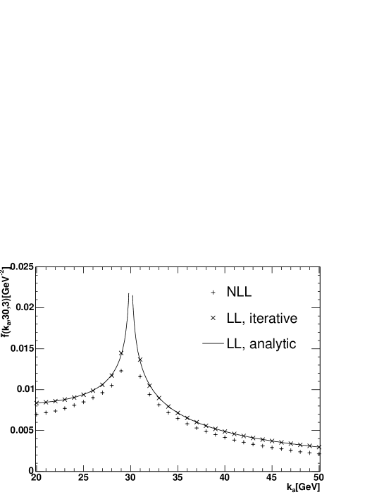
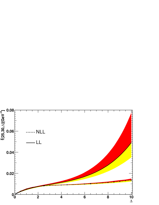
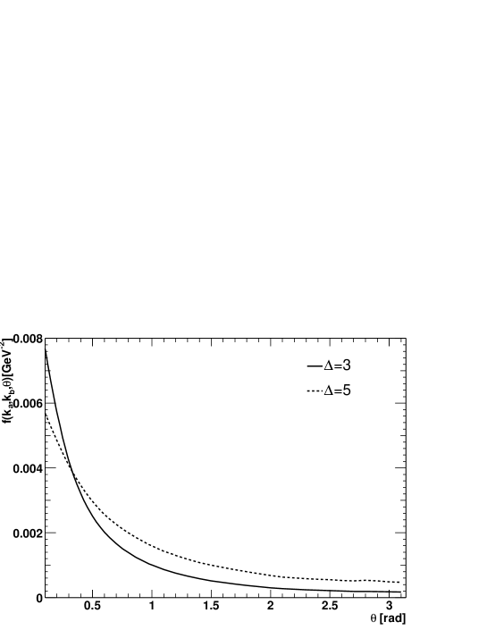
19.2 BFKL Phenomenology at Colliders 282828Contributing authors: J. R. Andersen, V. Del Duca
When confronting BFKL predictions with data, several points are worth observing. First of all, present day colliders do not operate at “asymptotic energies” where the high energy exponent dominates the BFKL prediction, leading to a prediction of an exponential rise in cross section with an intercept of . The logarithms resummed are kinematically generated, and in the derivation of the standard analytic solution to the BFKL equation, the transverse momentum of the gluons emitted from the BFKL evolution has been integrated to infinity. It is therefore apparent that any limits on the phase space probed in an experiment can have a crucial impact on the theoretical prediction. Such limits can either be the cuts implemented in the measurement or the overall limit on the available energy at a collider. Taking hadronic dijet production as an example, the energy constraint will obviously not just limit the possible rapidity separation of the leading dijets, but also the amount of possible radiation from the BFKL evolution, especially so when the leading dijets are close to the kinematical boundary. For a multi–particle final state described by two leading dijets with transverse momentum and rapidity and gluons described by , the square of the total energy of the event is given by where is the energy of the hadron collider and
| (44) |
where the minus sign in the exponentials of the right–hand side applies to the subscript on the left–hand side. Since in the analytic BFKL approach the contribution to from the BFKL radiation is inaccessible, this approach systematically underestimate the exact value of the ’s, and can thus grossly overestimate the parton luminosities.
The iterative approach of Refs.[211, 212] to solving the LL BFKL equation solves this problem. The results of this approach coincides with the LL limit of the solution of the NLL BFKL equation of Sec. 19.1. At LL the change in the –channel momentum at each step in the iteration corresponds to the momentum carried by one emission. The method therefore allows for the reconstruction of the full final state configurations contributing to the BFKL evolution, and it is possible to study quantities such as multiplicities and distribution in transverse momentum of the emitted gluons [213]. Only this reconstruction of the full final state allows for the observation of energy and momentum conservation. The effects of energy and momentum conservation have been studied in several processes [214, 215, 216]. When no phase space constraints are imposed, the iterative solution reproduces the known analytic solution to the LL BFKL equation.
In Ref. [215] we have, in light of the recent D0 measurement, re–analysed the Mueller–Navelet proposal of the study of dijets at hadron colliders in search of BFKL signatures. The main result of this study is that the difference between D0 and the Mueller–Navelet analysis in the reconstruction of the parton momentum fractions, the presence of an upper bound on the momentum transfer, and the contribution of the BFKL gluon radiation to the parton momentum fractions (at Tevatron energies) lower the parton flux in such a way as to approximately cancel the rise in the subprocess cross section with increasing dijet rapidity separation ()) predicted from the standard BFKL approach. This strong pdf suppression is due to the dijet production being driven by the gluon pdf, which is very steeply falling in for the region in of interest. This means that even the slightest change in has a dramatic impact on the parton flux and thus the prediction for the cross section. Also, the experimental cuts implemented have been shown to invalidate the Mueller–Navelet analysis and extraction of a ’BFKL intercept’.

As shown by this analysis, the expected rise in cross section over the LO QCD results does not survive once energy and momentum conservation is taken into account at the LHC or the Tevatron. However, other BFKL signatures should still be present; among those studied the most is the azimuthal decorrelation of dijets[217, 218]. In Fig. 46 we have plotted the data and prediction for the angular correlation between the leading dijets as a function of the inter–jet rapidity separation at the Tevatron. It should be noted that no detailed jet definition was applied in the BFKL prediction. It is, however, believed that a proper implementation of a jet finding algorithm will not change the partonic LL BFKL prediction significantly, since the gluons emitted from the BFKL evolution are typically well separated in rapidity. It is seen from Fig. 46 that the BFKL prediction respecting energy and momentum conservation is predicting slightly too much azimuthal decorrelation, but far less than an estimate based on a naive LL BFKL analysis ignoring the energy taken up by the BFKL radiation. On the other hand, a fixed NLO analysis shows too little decorrelation, while the prediction from HERWIG is in agreement with data. This shows that the decorrelation is dominated by soft gluon effects.
19.3 Experimental Opportunities at the LHC 292929Contributing authors: A. De Roeck
Studies of low- and BFKL dynamics at colliders typically require experiments with a large acceptance. Presently five experiments are planned at the LHC. Two of these, CMS [219] and ATLAS [220] are general purpose experiments with an acceptance in pseudorapidity of roughly for tracking based measurements and for calorimeteric based measurements. Here is defined as , with the polar angle of the particle. Hadronic jets can be detected and measured up to approximately while muons and electrons can be identified up to about . Extensions of the detector range are being investigated, as discussed below.
The TOTEM experiment [221] will use the same interaction point as the CMS experiment. TOTEM is an experiment to measure the elastic and total cross section and will use roman pot detectors to measure scattered protons in elastic and diffractive interactions, and charged particle detectors for tagging inelastic events in the regions (T1) and (T2). CMS is studying to add a calorimeter, called CASTOR, in the forward region directly behind T2. CASTOR will have an electromagnetic and hadronic readout section and an acceptance in the range . The TOTEM trigger and data readout will be such that these can be included in the CMS datastream, such that both experiments can run as one experiment. That way, a full detector with good coverage for jets and electrons/photons with rapidities of up to 7 will be available. The position of the T1, T2 trackers and the forward calorimeter, along the beamline and integrated with CMS, is shown in Fig. 47.
Roman pot detectors are presently also considered by ATLAS [222]. ATLAS further plans for a cerenkov/quartz fiber detector, called LUCID, for luminosity monitoring, which will cover the region . This detector could possibly be used for the tagging of rapidity gaps in an event.
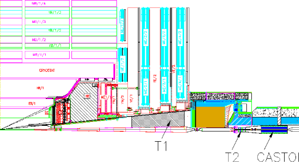
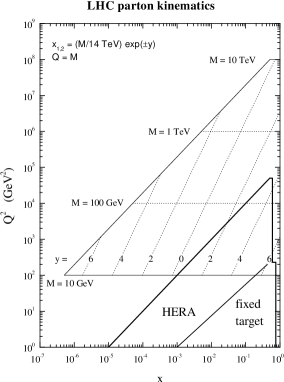
The extended coverage of the detectors will allow to probe processes at low- via Drell–Yan, jets, W and direct photon production. E.g. the Drell–Yan process has a simple experimental signature. The values of the two incoming quarks relate to the invariant mass of the two electron system as , hence when one of the values is large (say ), very low- can be probed with low mass Drell–Yan pairs. From Fig. 48 [223] we observe that in order to reach small masses (small scales) and low-, will require to probe large values of . Thus the resulting electrons will dominantly go in the very forward direction.
If low mass Drell–Yan pairs, prompt photons or jets (which have the same kinematics) can be measured in the CMS/TOTEM forward detectors, the parton distributions can be probed down to values of , i.e. at lower values than for any other collider. Depending on the low- dynamics, the predictions for jet, Drell–Yan and other cross sections can differ by a factor two or more in this region [224]. Experimental challenges on extracting the low- signals with respect to machine and QCD backgrounds are still under study.
The extended detector capabilities also allow for larger rapidity distances (i.e longer gluon ladders) between two measured hard jets, one of the golden BFKL measurements at a hadron collider (see Sec. 19.2). Note that the experiments will also measure all activity in between these two jets. Since BFKL does not have strong ordering the number and energy spectrum of the mini–jets produced along the ladder may be a significant footprint for BFKL. The main challenge will be to define a suitable trigger for this two jet channel. The presently foreseen trigger thresholds in ATLAS and CMS are around 150-200 GeV for one and two jet events, while for BFKL studies particularly jets in the energy range of 20-100 GeV are more of interest, since the distributions of these will be less distorted by kinematical constraints.
In principle it is also possible to run the LHC at lower energies, e.g. at 3 and 8 TeV, with significant luminosities (cm-2s-1), allowing to make parton density independent ratios of di–jet production at different energies, over a large range of rapidity.
For luminosities up to cm-2s-1 or below, the number of overlap events in one bunch crossing is small enough such that rapidity gaps can be used to detect interactions with colour singlet exchange [225]. The extended range covered in will allow to study events with multi–gaps. Hard diffractive phenomena, often linked to small- dynamics, can be studied further in detail via the tagging of the scattered protons in the roman pot detectors along the beam–line. Together with the measurement of the hard probes in the central LHC detectors, these events will allow for a detailed study of diffractive phenomena in collisions at the highest energies.
20 PION PAIR PRODUCTION AT THE LHC: COMPARING QCD@NLO WITH PYTHIA 303030Contributed by: T. Binoth, K. Lassila-Perini
20.1 Introduction
The indirect mass bounds for the Higgs boson from precision measurements indicate that the favoured range is below 200 GeV. A prominent search channel for neutral Higgs bosons in the mass window 80 GeV 140 GeV is the rare decay , as electromagnetic signals are preferable compared to hadronic ones due to huge backgrounds for the latter. The important backgrounds for this channel are prompt di-photon production and processes with one real photon and a jet with an isolated neutral meson. In addition, the abundant two jet rate at the LHC leads to a large reducible background where a meson in both jets produces an electromagnetic signature in the detector. This background needs to be rejected very efficiently. It is thus an important question to predict the respective rates as precisely as possible to allow for reliable simulations.
Experimental studies dominantly use PYTHIA [10] to predict the reaction rates for signal and background processes. PYTHIA is based on leading order matrix elements combined with initial and final state parton showers coupled to a hadronization model. One can expect that calculations in next-to-leading order in the QCD coupling lead to an improvement of the predictions in two respects. Firstly, distributions which are sensitive to hard radiation of an extra parton will not be described properly by a parton shower which is on the other hand expected to describe the collinear regions in phase space more reliably than a fixed order calculation. Secondly, inclusion of loop effects typically reduces the dependence on unphysical scales and thus leads to more reliable predictions.
The experimental studies show that the reducible pion+photon and di-pion contribution can be reduced by isolation cuts to a level which is acceptable for Higgs searches in the two photon channel [226, 227]. It is the aim of this study to cross check if this statement holds also at next-to-leading order (NLO) precision. We compare in the following production rates of pion pairs at high calculated with PYTHIA and the DIPHOX code [228]. The latter contains partonic matrix elements at NLO for the production of photon pairs, photon+hadron and hadron pairs and is flexible enough to account for diverse experimental cuts which can be modeled on the partonic level. For the description of hadrons in DIPHOX the model of collinear fragmentation is used. Partonic matrix elements are folded with fragmentation functions, which stand for the probability to find a hadron with an energy fraction relative to the jet formed by the initial parton . This probability is scale dependent. The scale dependence is governed by Altarelli-Parisi evolution. Initial distributions are fitted to experimental data in a certain range and extrapolated to the high (low) x range by some standard parameterizations. We note at this place that in the case of severe isolation cuts typically the tails of the fragmentation functions become numerically important which are not experimentally well restricted [229].
DIPHOX has been confronted with many different data sets from fixed target experiments to Tevatron data and showed an excellent agreement between di-pion or di-photon observables, whenever the condition for fixed order perturbative calculations were fullfilled [228, 230, 231]. We are thus in a situation to make a NLO prediction for photon pair, photon+pion and pion pair production at the LHC [229, 232, 233]. We want to mention that there is another calculation for di-hadron production at NLO available [234]313131In [176] corrections for two photon production via a quark loop at the two-loop level are taken into account..
A similar study for photon+pion production was presented by us in a previous Les Houches report [134]. We found good agreement between PYTHIA and DIPHOX for loose isolation cuts whereas for severe isolation cuts the PYTHIA rates were above the NLO predictions. Qualitatively we observed that isolation cuts are more efficient for the NLO calculation than in the PYTHIA result. We were lead to the conclusion that the experimental studies are conservative for the photon pion background.
20.2 Comparison: PYTHIA VS. DIPHOX
The basic underlying reaction for the production of pion pairs at leading order is two jet production with numerous different subprocesses like , , , , . It is a priori not clear, if there is a dominant process for different kinematical regions and experimental cuts. All subprocesses have to be considered. At NLO virtual corrections to the processes have to be combined with numerous matrix elements with one unresolved particle. Details of the calculation can be found in [228].
We compared two distributions relevant for Higgs boson searches, first the invariant mass distribution of the pion pair, with and second the transverse momentum distribution of the pion pair, with .
PYTHIA [10] version 6.205 was used to generate the events. High QCD processes were simulated and the events with two neutral pions were accepted. The pions were required to have 25 GeV and to be in the pseudo-rapidity range of 2.5. The isolation was implemented by setting a threshold to the sum of of all particles (excluding the pion itself) in the isolation cone .
The default parameters were chosen, apart from the longitudinal fragmentation function, where a hybrid scheme was used and for the multiple parton interactions, where a set of parameters tuned with the collider data [235] were used. The pile-up effects from collisions within the same bunch crossing were not taken into account, as we are here basically interested in a comparison of event rates of partonic interactions. We note that the multiple interactions belong to the regime of soft QCD, which is modeled in PYTHIA. The relevance of multiple interactions is restricted to values which are much below the scales used in our study. We are not in a regime where these effects are expected to become numerically sizable.
As already mentioned DIPHOX contains all matrix elements indicated above together with their next-to-leading order virtual and real emission corrections. Using the same experimental cuts defined above, the same distributions as with PYTHIA were produced by varying the renormalization (), factorization () and fragmentation () scales. We took with . For the parton distribution functions we used [236], for the pion fragmentation function we used a recent parametrization of Kramer, Kniehl and Pötter (KKP) [237] and an older one from Binnewies, Kramer and Kniehl (BKK) [238]. This was done to get an idea about the uncertainties due to fragmentation functions, although the KKP set should be more reliable, as it contains newer data.
In Fig. 49 we show the invariant mass distribution for two different isolation criteria, GeV in a cone . LO and NLO matrix elements were used for the DIPHOX predictions for three different choices of the scales. Higher scales mean lower cross sections in the plot. In the left plot KKP fragmentation functions were used, on the right the BKK parametrization. The PYTHIA prediction is shown as a full line. One observes that for PYTHIA undershoots the DIPHOX curves considerably. For the KKP fragmentation functions there is difference between a factor 2 to 6 for LO and 3 to 6 for NLO matrix elements. By using the BKK fragmentation functions, LO matrix elements and high scales () the accordance is improved. For the harder isolation cut, , the PYTHIA prediction shows a fair agreement with the DIPHOX result for both fragmentation functions. It is inside the scale variation of the NLO result apart for the last bin which is slightly below in the KKP case. One observes that the isolation cut acts more efficiently in DIPHOX than in PYTHIA. This was observed already in a earlier study [134]. It has to do with the different fragmentation models used. For more severe isolation preliminary results indicate that the PYTHIA distributions start to fall below the DIPHOX curves 323232The curve for GeV is not included because more statistics is needed to make a definite statement..
The inclusion of NLO matrix elements increases the cross section. In Fig.50 the ratio of NLO and LO result for KKP (left figure of Fig.49) is shown. Evidently the K-factors defined as this ratio depend on the scale choice and the experimental cuts, they vary between 1 and 2 for GeV and 2 and 3 for GeV, see Fig. 50. The inclusion of higher order terms improves the stability of the DIPHOX prediction under scale variations. This is much less pronounced for the harder isolation cut with GeV. Here compensations between LO and NLO terms are spoiled by the isolation cut. We note that asymmetric cuts, not applied here, lead to larger K-factors for the same reason [233].


Finally we present the transverse momentum distribution of the pion pair in Fig. 51. Now, only the NLO prediction is shown as this distribution is sensitive to matrix elements not present in the LO calculation. For a partonic reaction there is a kinematical restriction . Distributions beyond this point are filled by the parton shower in the PYTHIA case and with hard matrix elements in DIPHOX which are not present in PYTHIA. For GeV this does not affect the plotted range. Again, whereas PYTHIA undershoots the NLO curves considerably for GeV, the shape is very similar. Fair agreement is found for GeV for not too high values of . The drop in statistics of the PYTHIA curve can be understood by the missing matrix elements which are important for high values in the case of hard isolation.
20.3 Conclusion
We have presented a comparison between PYTHIA version 6.205 and DIPHOX version 1.2 for the pair production of high pions at the LHC. This is an important reducible background for Higgs search in the two photon channel. We observe that for loose isolation cuts the NLO result of DIPHOX is significantly higher than from PYTHIA which is due to matrix elements not present in PYTHIA and different fragmentation models in both codes. As isolation cuts act harder in DIPHOX than in PYTHIA, due to different fragmentation models, there is a fair agreement of both codes for a harder isolation cut. The trend is that for more severe isolation cuts PYTHIA will even overshoot the NLO predictions. We note that a further suppression of the dipion rate than shown in our plots is possible for example by using asymmetric cuts and pion/photon identification methods, but this is beyond the scope of this study.
We arrive at the tentative conclusion that experimental studies based on PYTHIA seem to be slightly below the more complete NLO calculation although the discrepancie is not dramatic. We have to stress that this statement depends strongly on the behaviour of the fragmentation model. Hard isolation means that fragmentation models are tested at high (the ratio between the pion energy and the jet energy). Currently the fragmentation functions are not well constrained experimentally in the high tails. Hopefully the situation improves soon by analyzing high pions at the Tevatron. Our study strongly motivates a refitting of the fragmentation functions which eventually leads in turn to a good understanding of the two photon rate at the LHC which is, apart from Higgs search, an interesting observable concerning our understanding of QCD.
Acknowledgements
We would like to thank Sasha Nikitenko for many useful discussions and also the conference organizers for the pleasant workshop.
21 QCD-INDUCED SPIN PHENOMENA IN TOP QUARK PAIR PRODUCTION AT THE LHC 333333Contributed by: W. Bernreuther, A. Brandenburg, Z.G. Si, P. Uwer
21.1 Introduction
The NLO QCD corrections to hadronic production have been known for quite some time [239, 240, 241, 242]. These results were refined by resummation of soft gluon [243] and threshold [244, 102] logarithms. These predictions were made for the production of pairs averaged over their spins. Because of the extremely short top-quark lifetime the spin properties of top quarks are transferred to its decay products without being diluted by hadronization. Thus quantities that involve the and/or spin are also “good” observables in the sense that they can be reliably calculated perturbatively, in particular within perturbative QCD. It is expected that such observables will be very useful in exploring the interactions that are involved in top quark production and decay. Besides standard model (SM) studies they allow, for instance, the search for non-SM interactions, in particular CP violating interactions of top quarks [245, 246, 247], or to pin down the nature of heavy resonances that strongly couple to top quarks [248, 247], if such objects exist.
Needless to say, searches for new interactions with top spin observables will require, on the theoretical side, rather precise SM precictions. While SM interactions induce only small polarizations of and quarks in hadronic production, the QCD-induced correlation between the and spins is large. They can be studied both at the Tevatron and at the LHC by means of double differential angular distributions of decay products. In this contribution we present results [249, 250, 251, 252] for these distributions at NLO QCD.
21.2 Theoretical framework
We consider hadronic production and subsequent decay into the following channels:
| (45) |
Here , , and denotes a jet originating from nonleptonic () decay. A complete next-to-leading order QCD analysis of (45) involves the parton reactions
| (46) |
| (47) |
| (48) |
where . In view of the fact that the total width of the quark is much smaller than its mass, , it is adequate to use the leading pole approximation (LPA) in calculating the NLO differential cross sections of the above parton reactions. Within the LPA, the radiative corrections can be classified into factorizable and non-factorizable contributions. The factorizable corrections were computed in [249, 250, 251, 252] in the narrow width approximation for which the contributions to the squared matrix element of the respective parton reaction are schematically of the form
| (49) |
Here denotes the density matrix which describes the production of on-shell pairs in a specific spin configuration, and are the density matrices describing the decay of polarised and quarks, respectively, into specific final states. The subscripts in (49) denote the , spin indices. The spin-averaged production density matrices yield the NLO cross sections for being produced by , , and fusion, which were first determined by [239, 240, 241, 242]. At NLO the and fusion reactions receive also non-factorizable corrections. They were computed by [253] in the semi-soft gluon approximation. While these contributions have an impact on, e.g., the and invariant mass distributions, they cancel in the integrated NLO cross sections of the above reactions [254, 255]. Moreover, it can be shown [252] that these non-factorizable corrections do not contribute either to the double differential distributions which will be discussed below. Therefore we will not discuss them here any further.
The factorizable contributions (49) must be consistently evaluated to order . This involves also the matrix elements to order of the main SM decay modes of the (anti)top quark in a given spin state, that is, the semileptonic modes , and the non-leptonic decays where for the dominant channels. For the computation of the double angular distributions (53) the matrix elements of the 2-particle inclusive parton reactions are required. Here denotes a lepton or a jet. In the LPA this involves the 1-particle inclusive decay density matrix where is the direction of flight in the rest frame and is the partial width of the respective decay channel. An analogous formula holds for decay. The factor is the spin analyzing power of particle/jet It is clear that its value is crucial for the experimental determination of top spin effects, in particular of spin correlations. For the standard charged current interactions these coefficients are known to order for semileptonic [256] and non-leptonic [257] modes. The charged lepton is a perfect analyzer of the top quark spin, which is due to the fact that
| (50) |
In the case of hadronic top quark decays the spin analysing power of jets can be defined. A detailed analysis was made in [257]; we give here only two examples:
| (51) | |||
| (52) |
where is the analysing power of the jet and refers to the least energetic non-b-quark jet defined by the Durham algorithm. Using hadronic final states to analyze the spins of and/or results in a loss of analyzing power. However, this is (over)compensated by the gain in statistics and by the efficiency with which the () rest frames can be reconstructed.
Let us now discuss double angular distributions for the channels (45) which are appropriate observables to measure the (QCD induced) spin correlations. Here is the angle between the direction of flight of particle/jet in the rest frame with respect to reference directions () which will be specified below. We define the rest frame by a rotation-free boost from the zero-momentum frame, for reasons given below. As mentioned above, non-factorizable corrections do not contribute, at NLO, to this type of distributions [252]. Thus, to this order in the QCD coupling () can be interpreted as spin quantization axes, see below. Integrating over the full phase space and choosing , as given below it can be shown [252] that these distributions have the generic form343434QCD (or SM) generated absorptive parts in the parton scattering amplitudes induce a small and polarization, which to order is normal to the scattering planes [258, 259].
| (53) |
The coefficient which signals the correlation between the spins depends, for a given reaction, on the choice of and For the factorizable corrections the exact (to all orders in ) formula holds [251]. Here is the double spin asymmetry
| (54) |
where denotes the number of pairs with () spin parallel to the reference axis (), etc. Thus and can be identified with the quantization axes of the and spins, respectively, and directly reflects the strength of the correlation between the and spins for the chosen axes.
For production at the Tevatron it is well known that the so-called off-diagonal basis [260], which is defined by the requirement that for the process at tree level, yields a large coefficient . It has been shown in [251] that the beam basis, where and are identified with the hadronic beam axis, is practically as good as the off-diagonal basis. A further choice is the helicity basis, which is suitable for the LHC.
An important theoretical issue of top quark spin physics beyond leading-order QCD is the construction of infrared and collinear safe observables at the parton level. In the case at hand it boils down to the question in which frame the reference directions and are to be defined. It has been shown [252] that, apart from the and rest frames, the zero momentum frame (ZMF) is the appropriate frame for defining collinear safe spin-momentum observables. The off-diagonal, beam, and helicity bases which we refer to in the next section are defined in the ZMF. Details will be given in [252].
21.3 Spin correlations at nlo: predictions for the Tevatron and the LHC
We have computed the 2-particle inclusive differential cross sections for (45) and, in particular, the double angular distributions (53) to NLO QCD, with and the top mass being defined in the and in the on-shell scheme, respectively. The mass factorization was performed in the scheme.)
In Table 3 we list our predictions [252] for the spin correlation coefficient in the double differential distribution (53) at the Tevatron for the three different choices of references axes discussed above. We use the CTEQ6L (LO) and CTEQ6.1M (NLO) parton distribution functions (PDF) [171]. Numbers are given for the dilepton, leptonjet and all-hadronic decay mode of the pair, where in the latter two cases the least energetic non--quark jet (defined by the Durham cluster algorithm) was used as spin analyser. One sees that the spin correlations are largest in the beam and off-diagonal basis. The QCD corrections reduce the LO results for the coefficients by about 10% to 30%.
| dilepton | lepton+jet | jet+jet | ||
|---|---|---|---|---|
| LO | 0.471 | 0.240 | 0.123 | |
| NLO | 0.352 | 0.168 | 0.080 | |
| LO | 0.928 | 0.474 | 0.242 | |
| NLO | 0.777 | 0.370 | 0.176 | |
| LO | 0.937 | 0.478 | 0.244 | |
| NLO | 0.782 | 0.372 | 0.177 |
For the LHC it turns out that the spin correlations w.r.t. the beam and off-diagonal basis are quite small due to a cancellation of contributions from the and initial states. Here, the helicity basis is a good choice, and Table 4 shows our results for the coefficient in that case. The QCD corrections are smaller for the LHC than for the Tevatron; they vary between 1 and 10. For both colliders the relative corrections are largest for the all-hadronic decay modes and smallest for the dilepton decay modes.
| dilepton | lepton+jet | jet+jet | ||
|---|---|---|---|---|
| LO | 0.319 | 0.163 | 0.083 | |
| NLO | 0.326 | 0.158 | 0.076 |
An interesting aspect of these double distributions is their high sensitivity to the quark and gluon content of the proton [251]; the reason being that the contributions to from and initial states have opposite signs. Table 5 shows, for dilepton final states, the dependence of the NLO results on the choice of the PDF. While the results for the recent CTEQ6.1M and MRST2003 [261] PDF agree at the percent level (this is not the case for previous versions of the CTEQ and MRST PDF), the GRV98 [262] PDF give significantly different results at the Tevatron. This shows that measurements of (53) may offer the possibility to further constrain the quark and gluon content of the proton.
| Tevatron | |||
| CTEQ6.1M | MRST2003 | GRV98 | |
| 0.352 | 0.351 | 0.313 | |
| 0.777 | 0.777 | 0.732 | |
| 0.782 | 0.782 | 0.736 | |
| LHC | |||
| 0.326 | 0.327 | 0.339 | |
All the results above were obtained with GeV. A variation of the scale between and changes the central results for at by roughly . Varying from to GeV changes the results for at the Tevatron by less than , while for the LHC, changes by less than a percent.
21.4 Conclusion
Top-antitop spin correlations, which are predicted to be large within the SM, are expected to become a good tool for analyzing in detail top quark pair production and decay dynamics. They can be studied at the Tevatron and – in view of the expected large data samples – especially at the LHC in the dilepton, single lepton and all-hadronic decay channels by measuring suitably defined double angular distributions. While the NLO QCD corrections to these distributions are of the order of 10 to 30 for the Tevatron, they are below 10 for the LHC. Work on soft gluon and threshold resummations will further reduce the theoretical uncertainties.
22 QCD RADIATIVE CORRECTIONS TO PROMPT DIPHOTON PRODUCTION IN ASSOCIATION WITH A JET AT THE LHC 353535Contributed by: V. Del Duca, F. Maltoni, Z. Nagy, Z. Trócsányi
22.1 Introduction
Higgs production in association with a jet of high transverse energy with a subsequent decay into two isolated photons, , is considered a very promising discovery channel for a Higgs boson of intermediate mass (100 GeV 140 GeV) [263, 264, 265]. The main background to this signal is the channel, where the photons are isolated. In this channel the signal is a small and narrow peak on a flat background [265]. Thus the QCD prediction is not needed for predicting the background, which can be well measured from the sidebands, but rather to optimize the selection and isolation cuts for the experimental search. For this purpose usually a Monte Carlo program is used [70], which however, does not take into account the QCD radiative corrections. These corrections are large and strongly dependent on the photon isolation parameters [265] and therefore cannot be ignored in the analysis.
In perturbative QCD, the cross section for the production of a single isolated photon in a collision of two hadrons and of momenta and , respectively, has the following general form:
| (55) |
The first term is called the direct component, where the subtracted partonic cross sections get contributions from all the diagrams with a photon leg. The second term is called fragmentation component, where the subtracted partonic cross sections get contributions from diagrams with only coloured external partons, with one of the partons eventually fragmenting into a photon, in a way described by the (perturbatively uncalculable but universal) parton-to-photon fragmentation function . If there are two isolated photons, the equation contains four terms, a double direct, two single-fragmentation and a double-fragmentation component [228]. The direct and fragmentation components are not defined unambiguously (except for the case of the ‘smooth’ photon isolation to be used here), finite terms can be shifted among the terms, only the sum is meaningful physically. The precise definition of the direct and fragmentation terms, valid to all orders in perturbation theory, can be found for instance in Ref. [266].
In perturbation theory beyond leading order, the isolated photon cross section is not infrared safe. To define an infrared safe cross section, one has to allow for some hadronic energy inside the photon isolation cone. In a parton level calculation it means that soft partons up to a predefined maximum energy are allowed inside the cone. This is also natural in the experiment: complete isolation of the photon is not possible due to the finite energy resolution of the detector.
There are two known ways to implement the photon isolation. The standard way of defining an isolated prompt photon cross section, that matches the usual experimental definition, is to allow for transverse hadronic energy inside the photon isolation cone up to , with typical values of between 0.1 and 0.5363636In experiments, often a fixed value of in the order of several GeV is used., and where is taken either to be the photon transverse momentum on an event-by-event basis or to correspond to the minimum value in the range. Using this isolation prescription, both the direct and the fragmentation terms contribute to Eq. (55). In Ref. [266] it was shown that a small isolation cone for the photon leads to unphysical results in a fixed order computation. For a small cone radius , an all-order resummation of terms combined with a careful study of the border line between perturbative and non-perturbative regions has to be undertaken.
Even with resummation, the very narrow isolation cone is not favoured from the practical point of view. The ratio of the fragmentation component to the direct one slowly increases with decreasing . Since the fragmentation function is non-perturbative, therefore, it has to be measured and the available functions have relatively large errors. The fragmentation component is also strongly dependent on , increasing rapidly with increasing . Thus, the theoretical uncertainty related to the photon fragmentation can be decreased with large cone sizes and small .
In order to avoid completely the uncertainties related to the fragmentation component, Frixione introduced a ‘smooth’ photon-isolation when the fragmentation contribution is zero [267]. This isolation means that the energy of the soft parton inside the isolation cone has to converge to zero smoothly if the distance in the plane between the photon and parton vanishes. Explicitly, the amount of hadronic transverse energy (which in our NLO partonic computation is equal to the transverse momentum of the possible single parton in the isolation cone) in all cones of radius must be less than
| (56) |
The smooth isolation prescription can be viewed as if the singularity in the quark-photon splitting were factorized into the fragmentation component using phase-space cuts such that the finite remainder in the fragmentation is shifted completely into the direct component in a perturbatively computable way.
The two prescriptions have their own advantages and less appealing features. The standard isolation is easier to employ experimentally, but has the following disadvantages from the theoretical point of view: (i) it involves a non-perturbative component in its theoretical prediction (fragmentation) with large errors due to pure experimental information; (ii) the theoretical prediction of the fragmentation is more difficult to compute than that of the direct component. The smooth isolation is easier to implement in NLO perturbation theory. However, it is less favoured in the experiment because (i) it is difficult to employ it due to the finite granularity of the detector; (ii) it was found to be less efficient for isolating photons from jets than the cone isolation, approaching the efficiency of the latter with tending to zero [268].
Experimentally the standard cone isolation is recovered from the smooth isolation when . The smooth isolation leads to smaller cross sections for the same values of the cone radius and , because it means a more severe cut into the phase space. However, due to the finite granularity of the detector, the two prescriptions yield equal cross sections even for small, but non-zero values of . Small values of can be chosen in perturbation theory, but cannot be taken without including the fragmentation component. If we are interested only in the Higgs-boson search, we need a perturbative prediction that is reliable for those values of the isolation parameters which are found useful to increase the signal significance. Studying the dependence of the perturbative prediction with the smooth prescription on the isolation parameters, we can estimate the reliability of the theoretical predictions.
In order to assess the dependence of the radiative corrections on the isolation parameters, we use a partonic Monte Carlo program which employs the dipole subtraction method [269], slightly modified for better numerical control [270] as implemented in the NLOJET++ package [271], and use the smooth isolation prescription at the parton level. We compute cross section values at leading order and at NLO for a Large Hadron Collider (LHC) running at 14 TeV. The values shown at leading order were obtained using the leading order parton distribution functions (p.d.f.’s) and those at NLO accuracy were obtained using the NLO p.d.f.’s of the CTEQ6 package [98] (tables cteq6l1 and cteq6m, respectively). We used the two-loop running of the strong coupling at NLO with MeV and one-loop running with MeV at leading order. The renormalization and factorization scales are set to , where for the reference value we use with the invariant mass of the photon pair. This definition reduces to the usual scale choice for inclusive photon pair production if vanishes. Our prediction for the production cross section is intended for use in the detection of a Higgs boson lighter than the top quark, therefore, we assume 5 massless flavours and restrict all cross sections to the range of 80 GeV 160 GeV. The electromagnetic coupling is taken at the Thomson limit, . We use a jet reconstruction algorithm and a set of event selection cuts, expected to be typical in Higgs searches. In particular, in order to find the jet, we use the midpoint cone algorithm [272] with a cone size of , with the rapidity interval and the azimuthal angle373737In our NLO computation the midpoint and seedless cone algorithms yield identical cross sections.. Then, we require that both the jet and the photons have GeV and rapidity within . These are the same selection cuts as used in Ref. [273] for computing the gluon initiated corrections. Furthermore, we isolate both photons from the partons in a cone of size .
22.2 Results
In Fig. 52(a) we plot the invariant mass distribution of the photon pair. Here we see the continuum background on which the Higgs signal is expected to manifest itself as a narrow resonance in the intermediate-mass range. The dotted (red) line is the leading order prediction and the solid (red) one is the differential cross section at NLO accuracy. The striking feature of the plot is the rather large correction. The large corrections are partly due to the appearance of new subprocesses at NLO as can also be read off the figure. The gluon-gluon scattering subprocess begins to appear only at NLO accuracy, and therefore it is effectively leading order. It is shown with a long dashed-dotted (magenta) line: it yields a very small contribution. The bulk of the cross section comes from quark-gluon scattering both at leading order and at NLO, shown with sparsely-dotted (blue) and long-dashed (blue) lines. The quark-quark scattering receives rather large corrections because the leading order subprocess can only be a quark-antiquark annihilation process, shown with short-dashed (green) line, while at NLO, shown with short dashed-dotted (green) line, there are (anti-)quark-(anti-)quark scattering subprocesses. Thus at NLO the parton luminosity is sizeably larger. In addition, more dynamic processes are allowed, which include -channel gluon exchange. These contribute to enlarge the cross section in phase space regions which are disfavoured at leading order.
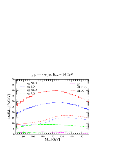
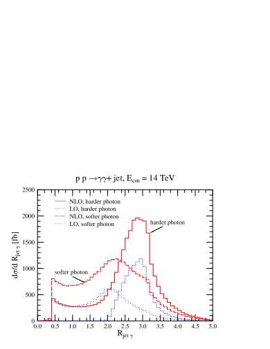
A part of the large radiative corrections is accounted for by the new subprocesses; another part is due simply to the enlarged phase space, as can be seen from of Fig. 52(b), where the differential distributions in the distance between the jet and the photons in the - plane are shown, with a selection cut at . From the distribution for the harder photon we see that the radiative corrections recieve contributions from a larger part of the phase space than the prediction at leading order. In fact, on one hand a cut on affects the leading order and the NLO evaluation in the same way because they have the same shape. Thus in that case the cut does not reduce the correction to the distribution. On the other hand, a cut on cuts the NLO correction, but does not cut the leading order, so the correction is reduced. Nevertheless, the reduction is less then 10 %, thus cutting on at reduces the NLO correction to the invariant mass distribution of the photon pair, but marginally. In the rest of this study we require and GeV, in addition to the same selection cuts as used in Fig. 52.
Next we consider the dependence of the isolated cross section on the power in the definition of the smooth isolation Eq. (56). We show the dependence on for , and , in Fig. 53(a). We see that the radiative corrections are much more than 100 % and depend on strongly if the isolation cone is narrow and is large, therefore, the fixed-order perturbative prediction at the NLO accuracy is not reliable in this case. On the other hand, the dependence on is much milder and remains well below 100 % for , . Thus, the line can be considered a good approximation to the prediction with standard photon isolation.
In order to assess the stability of the predictions against scale variations, we show the cross section in a 3 GeV bin around GeV, that is the background for a hypothetical Higgs signal for a Higgs particle of mass 120 GeV. Fig. 53(b) shows the cross section for two sets of photon-isolation parameters. We show the scale variations for varying the renormalization and factorization scales separately, keeping the other scale fixed, as well as varying them simultaneously. The lower three curves represent the leading order predictions. At leading order the dependence on the renormalization and factorization scales is rather small, especially when the two scales are set equal (densely dotted line). Observing the predictions we conclude that the scale dependence at leading order does not represent the uncertainty of the predictions due to the unknown higher orders. The inclusion of the radiative corrections results mainly in the substantial increase of the cross section. For the isolation parameters and the NLO corrections at are about 120 % of the leading order prediction. In addition, the scale dependence is not reduced by the inclusion of the radiative corrections. If we require more stringent photon isolation cuts, then we find smaller corrections and a more stable prediction. For instance, in Fig. 53(b) we also show the scale dependence of the cross section obtained with and . We find that the cross section at NLO is about 40 % larger than the leading order prediction, and in this case the scale dependence at NLO is reduced as compared to the one at leading order accuracy. The reduction of the scale dependence when the stronger cuts ( with ) are used indicates that the large correction obtained with the looser (default) cuts are due mainly to real emission of soft and collinear partons.
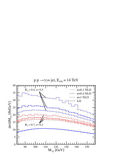
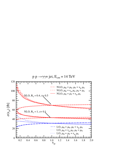
22.3 Conclusions
We conclude by summarizing our observations concerning the QCD radiative corrections to the process that constitutes part of the irreducible background to the discovery channel of an intermediate-mass Higgs boson at the LHC. We used a smooth photon isolation that is infrared safe to all orders in perturbation theory and independent of the photon fragmentation into hadrons. We found large radiative corrections, which are rather sensitive to the selection cuts and photon isolation parameters. Choosing a mild photon isolation, i.e. a small isolation cone radius with relatively large hadronic activity allowed in the cone results in more than 100 % correction with as large residual scale dependence at NLO as at leading order. In this case, the dependence on the isolation parameter is also large. Since the radiative correction with standard photon isolation would even be larger, we conclude that NLO perturbation theory does not yield a reliable theoretical prediction for such a mild photon isolation. Making the photon isolation more stringent, for instance increasing the cone radius to and decreasing the hadronic activity in the cone (using for instance ) reduces both the magnitude of the radiative corrections as well as the dependence on the renormalization and factorization scales and that on the isolation parameter . The more stringent isolation is also useful for decreasing the relative weight of the poorly known fragmentation components in the cross section, and the prediction obtained with the smooth isolation can be considered a good approximation (valid to the extent of scale ambiguities) to those with the standard isolation. Our results show that a constant factor is not appropriate for taking into account the radiative corrections to the irreducible background of the discovery channel at the LHC.
Acknowledgments
This work was supported in part by US Department of Energy, contract DE-FG0396ER40969 and by the Hungarian Scientific Research Fund grants OTKA T-038240.
23 ELECTROWEAK RADIATIVE CORRECTIONS TO HADRONIC PRECISION OBSERVABLES AT TEV ENERGIES 383838Contributed by: E. Maina, S. Moretti, M.R. Nolten, D.A. Ross
23.1 Weak corrections at TeV scales
At TeV energy scales, next-to-leading order (NLO) Electro-Weak (EW) effects produce leading corrections of the type , where , with the Electro-Magnetic coupling constant and the Weinberg angle. In fact, for large enough values, the centre-of-mass (CM) energy at parton level, such EW effects may be competitive not only with next-to-NLO (NNLO) (as ) but also with NLO QCD corrections (e.g., for TeV, ).
These ‘double logs’ are due to a lack of cancellation between virtual and real -emission in higher order contributions. This is in turn a consequence of the violation of the Bloch-Nordsieck theorem in non-Abelian theories [274]. The problem is in principle present also in QCD. In practice, however, it has no observable consequences, because of the final averaging of the colour degrees of freedom of partons, forced by their confinement into colourless hadrons. This does not occur in the EW case, where the initial state has a non-Abelian charge, as in an initial quark doublet in proton-(anti)proton scattering. Besides, these logarithmic corrections are finite (unlike in QCD), since provides a physical cut-off for -emission. Hence, for typical experimental resolutions, softly and collinearly emitted weak bosons need not be included in the production cross section and one can restrict oneself to the calculation of weak effects originating from virtual corrections only. By doing so, similar logarithmic effects, , are generated also by -boson corrections. Finally, all these purely weak contributions can be isolated in a gauge-invariant manner from EM effects which therefore may not be included in the calculation. In fact, we have neglected the latter here.
In view of all this, it becomes of crucial importance to assess the quantitative relevance of such weak corrections affecting, in particular, key QCD processes studied at present and future hadron colliders. We show here results for the case of -jet-, prompt-photon and -production at Tevatron and LHC.
23.2 Corrections to -jet-production
In Fig. 54 (left and right panels) we show the effects of the full contributions to the and cross sections at Tevatron and LHC, respectively. (For details of the calculation, see Ref. [275].) Results are shown for the total inclusive -jet production rate as a function of the jet transverse energy. (Tree-level EW and NLO QCD effects are also given for comparison.) At Tevatron, terms are typically negligible in the inclusive cross section, as the partonic energy available is too small for the mentioned logarithms to be effective. At LHC, the contribution due to such terms grows accordingly to the collider energy, reaching the –2% level at transverse momenta of GeV.
Next, we study the forward-backward asymmetry at Tevatron, defined as follows:
| (57) |
where the subscript identifies events in which the -jet is produced with polar angle larger(smaller) than 90 degrees respect to one of the two beam directions (hereafter, we use the proton beam as positive -axis). The polar angle is defined in the CM frame of the hard partonic scattering. In the center plot of Fig. 54, the solid curve represents the sum of the tree-level contributions, that is, those of order and , whereas the dashed one also includes the higher-order ones . The effects of the one-loop weak corrections on this observable are rather large, indeed comparable to the effects through order [276, 277]. In absolute terms, the asymmetry is of order at the , resonance (i.e., for ) and fractions of percent elsewhere, hence it should be measurable after the end of Run 2. We expect even larger effects at LHC, however, some care is here necessary in order to define the observable, which depends on the configuration and efficiency of the experimental apparata (so we do not present the corresponding plot in this instance). The results presented here are from Ref. [278].


23.3 Corrections to - and -production
The neutral-current processes ()
| (58) |
are two of the cleanest probes of the partonic content of (anti)protons, in particular of antiquark and gluon densities. In order to measure the latter it is necessary to study the vector boson spectrum. That is, to compute production in association with a jet (originated by either a quark or a gluon). We briefly report here on the full one-loop results for processes (58) obtained through . (For technical details of the calculation, see Ref. [279].)
Fig. 55 shows the effects of the corrections relatively to the Born results ( replaces for photons), as well as the absolute magnitude of the latter, as a function of the transverse momentum. The corrections are found to be rather large, both at Tevatron and LHC, particularly for -production. In case of the latter, such effects are of order –10% at Tevatron and –15% at LHC for GeV. In general, above GeV, they tend to (negatively) increase, more or less linearly, with . Such effects are indeed observable at both Tevatron and LHC. For example, at FNAL, for -production and decay into electrons and muons with BR, assuming fb-1 as integrated luminosity, in a window of 10 GeV at GeV, one finds 650–6500 events through LO, hence a EW NLO correction corresponds to 10–100 fewer events. At CERN, for the same production and decay channel, assuming now fb-1, in a window of 40 GeV at GeV, we expect about 1200 events from LO, so that a EW NLO correction corresponds to 140 fewer events. In line with the normalisations seen in the top frames of Fig. 55 and the size of the corrections in the bottom ones, absolute rates for the photon are similar to those for the massive gauge boson while corrections are about a factor of two smaller.
Altogether, these results point to the relevance of one-loop contributions for precision analyses of prompt-photon and neutral Drell-Yan events at both Tevatron and LHC, also recalling that the residual scale dependence of the known higher order QCD corrections to processes of the type (58) is very small in comparison [280, 84, 281, 282]. Another relevant aspect is that such higher order weak terms introduce parity-violating effects in hadronic observables [283], which can be observed at (polarised) RHIC-Spin [284].
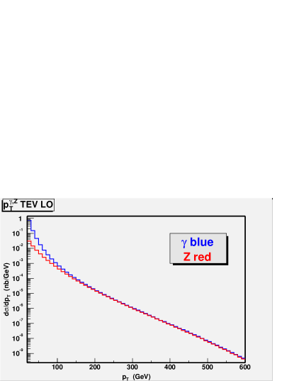
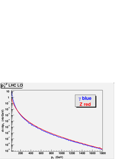
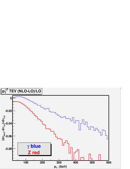
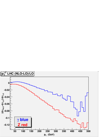
24 TOWARDS AUTOMATED ONE-LOOP CALCULATIONS FOR MULTI-PARTICLE PROCESSES 393939Contributed by: T. Binoth, J.Ph. Guillet, G. Heinrich, N. Kauer, F. Mahmoudi
24.1 Introduction
In this decade experiments at hadron colliders explore the TeV scale. The large center of mass energies lead generically to multi-particle final states created by QCD initial states. The application of perturbative methods is justified if the scales of the problem are considerably larger than the proton mass. Then a systematic separation of long and short distance effects is possible and predictions for cross sections can be made at the loop level, which is mandatory for a reliable estimate of production rates especially at hadron colliders.
The calculation of multi-particle production at the one-loop level is very challenging due to the combinatorial complexity of the Feynman diagrammatic approach. Although the calculation of partonic amplitudes at one-loop is meanwhile standard, already the number of known 1-loop amplitudes is very restricted. Up to now not a single Standard Model process which has generic kinematics is computed at the one-loop level. Needless to say this is highly relevant to many search channels for the Higgs boson at the LHC, like gluon fusion and weak boson fusion, where additional jets have to be tagged to improve the signal to background ratio. For signal reactions like jets, with which are available at one-loop level, not all amplitude calculations for the background exist. This is due to the fact that the signal case typically contains only 5-point functions at 1-loop, whereas the background has generic kinematics. As an example for such reactions consider , or . These require the evaluation of hexagon graphs like
The aim of our working group is to develop methods for the calculation of such hexagon amplitudes. The final goal is a tool to tackle the computation of general processes at the one-loop level in a completely automated way. A basic ingredient of such a tool are algebraic reduction formulas. Our reduction formalism is described in the next section. As an example for the efficiency of our methods we discuss the 5-point 1-loop amplitude in Section 24.3. The fully analytical treatment of hexagon one-loop amplitudes seems to be feasible analogously, if massless particles are considered. Examples of hexagon amplitudes in the Yukawa model calculated with our approach can be found in [285, 286]. Other, phenomenologically relevant examples are presently under study. For the massive case we suggest a numerical evaluation described in Section 24.4.
24.2 Reduction Formalism
We will very briefly discuss the basic reduction formulas for -point scalar and tensor integrals. More details can be found in [287, 288].
24.2.1 Tensor reduction
Feynman diagrams correspond to combinations of tensor integrals. The momentum space representation of an -point tensor integral of rank in dimensions is given by
| (59) |
Here is a linear combination of the loop momentum and external momenta . If standard reduction methods lead to a proliferation of terms with complicated denominators. This has to be avoided, as otherwise a stable numerical evaluation of the amplitude is hardly possible. By using helicity or projection methods loop momenta can always be combined with external momenta such that they are expressed by combinations of inverse propagators, e.g. with , , and :
| (60) |
After expressing products of loop momenta with external vectors by propagators and canceling as many propagators as possible, one is left with tensor integrals which are irreducible. One finds that at most rank 1 -point integrals have to be reduced for an -point problem. Explicit representations for the irreducible tensor integrals can be found in [288]. After complete tensor reduction one is left with a linear combination of scalar integrals.
24.2.2 Scalar reduction
To achieve as many analytic cancellations as possible the amplitude has to be expressed by a basis of scalar integrals. To this end scalar -point integrals have to be reduced further. The scalar -point function in momentum and Feynman parameter space is given by
| (61) |
where , , . The basic reduction formula relates an -point scalar integral to -point scalar integrals , where the th propagator is omitted, and -dimensional remainder terms:
| (62) |
The reduction coefficients are . One finds by iteration that each -point function and therefore each amplitude can be expressed by 2- and 3-point functions in dimensions and 4-point functions in dimensions only. These form the basic building blocks for an irreducible representation of the amplitude in terms of scalar functions. The coefficients of these scalar integrals are expected to simplify to a large extent.
24.3 Analytic Calculation of
To give an example for our algebraic approach to -point amplitudes we have reconsidered the 5-point 1-loop amplitude . While this amplitude only had been extracted indirectly from the 5-gluon amplitude [289] by replacing gluons by photons until recently, we present a direct calculation [290].
For convenience we define all particles as incoming.
| (63) |
Out-states can be obtained by crossing rules. In hadronic collisions this amplitude is relevant for the production of photon pairs in association with a jet and as such a contribution of the background to the Higgs boson search channel . A phenomenological analysis has already been provided in [273, 265]. The colour structure of this amplitude is simple. It can be written as
| (64) |
are helicity dependent linear combinations of scalar integrals and a constant term which is a remnant of two-point functions with coefficients of order . Six independent helicity components exist: +++++,++++ –,– ++++,– – +++, +++ – –, – +++ –. As the amplitude is finite one expects that all 3-point functions which carry spurious infrared poles cancel. The function basis of the problem is thus reduced to 2-point functions , 4-point functions in dimensions written as [286]
| (65) |
and constant terms. From unitarity one expects that the +++++ , ++++ – , – ++++ amplitudes should be polynomial. The other helicity amplitudes will also contain non-polynomial functions like logarithms and dilogarithms contained in and .
To give an example of each case we show here the results for and only, the remaining ones which have also compact representations can be found in [290]. The result is expressed in terms of field strength tensors which satisfy the relations
| (66) |
where are the polarization vectors of the gluons and photons.
For which is polynomial we find the following result
| (67) |
The coefficient is given by
| (68) | |||||
We have checked that the corresponding amplitude has a Bose symmetry when the photons and the gluons with equal helicities are interchanged.
For we split the result into three pieces with indices , which belong to the part proportional to 6-dimensional boxes , a part containing bubble graphs , and a constant term, respectively.
| (69) |
We find
| (70) |
The indicated permutations have to be applied to the indices of the field strength tensors, momenta and Mandelstam variables. The coefficients are
In the given expressions the symmetry under exchange of the two photons and the three gluons is manifest after taking into account the omitted colour factor.
The result indicates that with our approach indeed a compact representation of complicated loop amplitudes can be obtained. The application of our approach to relevant 6-point amplitudes is presently under study.
24.4 Numerical Evaluation of Multi-Leg Integrals
As already mentioned, our final aim is a complete automatisation of one-loop calculations. The bottleneck for this goal is mainly given by the calculation of the virtual amplitudes: As the number of external legs increases, the growing number of invariants renders the analytical expressions more and more complicated. If in addition massive particles are involved, the complexity of the resulting expressions rapidly approaches a limit where the analytical evaluation of the amplitude becomes unfeasible. Therefore, a numerical approach seems to be more appropriate to tackle different types of one-loop amplitudes in a unified and efficient way. Of course, it has to be stated what ”numerical” means, as any method should finally lead to ”numbers” to be compared to data. The important question is at what stage of the calculation the transition from analytical to numerical evaluation should be made.
The conventional approach to calculate NLO cross sections seeks to keep analytical expressions in the course of the calculation of a cross section as far as possible. Of course, there are good reasons to do so: If infrared (and/or ultraviolet) poles are present, they have to be isolated and canceled before any numerical evaluation can be attempted. Further, analytic expressions are flexible in the sense that they can be used in ”crossed” processes with different kinematics by analytic continuation. On the other hand, the analytical approach may be troublesome if the calculation of differential cross sections for some (infrared safe) observable and/or the implementation of experimental cuts requires modifications of the analytic expressions. In addition, concerning the virtual integrals, it is well known that even if a closed form exists, the implementation into a Monte Carlo program may lead to numerical instabilities because the expressions are not appropriate for every phase space region.
These drawbacks of the ”maximally analytical” approach suggest to make the transition analytical numerical at an earlier stage of the calculation. A completely numerical approach has been suggested by D. Soper [291, 292], where the sum over cuts for a given graph is performed before the numerical integration over the loop momenta, in this way exploiting unitarity to cancel soft and collinear divergences. This method is very elegant, but choosing appropriate integration contours in the multi-dimensional parameter space is far from straightforward and therefore might be hard to automate.
In [293], a different approach has been suggested, where the calculation is split into ”virtual” (loop) and ”real” contributions as in the conventional approach, but a subtraction formalism for the UV and soft/collinear divergences of the one-loop graphs has been worked out, such that the subtracted integrals can be performed numerically in four dimensions. While the subtractions act on a graph by graph basis, the subtraction terms are added back (in analytically integrated form) after having been summed over the graphs, as only the summation leads to expressions which are simple enough to be integrated analytically.
Another promising approach in this context is the one of [294], which tries to tackle the problem of infrared divergences by its very root: Starting from the observation that the clash between the long-range nature of the interactions in a massless gauge theory and the assumption of asymptotically free external states causes the appearance of IR singularities in the ”conventional” amplitudes, they show that an appropriate redefinition of the external states, which includes the long-range interactions, leads to S-matrix elements which are IR finite and apply it to the case jets at NLO.
The method we suggest here to calculate one-loop amplitudes is oriented at the aim of automatisation as a main guideline. It follows to a large extent the ”analytical road” in treating virtual and real emission corrections separately. This is feasible as the isolation of IR/UV divergences is straightforward if the discussed reduction formalism is used. UV renormalisation is well understood, and systematic methods for the combination of the IR divergences from the virtual corrections with their counterparts from the real emission contribution also exist [295, 281, 296, 297, 269, 298, 299]. The main problem consists in calculating the remaining finite terms of the -point one-loop amplitudes, especially for , and we will concentrate on this point in what follows. By making the transition from analytical to numerical evaluation for these terms at an earlier stage than in the conventional approach, complicated cancellations between numerous dilogarithms can be avoided.
We should mention that another approach to calculate loop integrals numerically is suggested by Passarino et al. [300, 301], based on the Bernstein-Tkachov relation [302].
24.4.1 Reduction to basic building blocks
A one-loop -point amplitude involving particles with arbitrary masses (including the case ) will be reduced to basic building blocks using the method of [288], as outlined in Section 24.2 As basic building blocks, we choose scalar 2-point functions and 3-point functions in dimensions and dimensional box functions . The latter are infrared finite. Possible UV singularities are only contained in the 2-point functions and their subtraction is straightforward. The (soft and collinear) IR singularities are, as a result of the reduction, only contained in 2-point functions and 3-point functions with one or two light-like legs. In this form, they are easy to isolate and to subtract from the amplitude. However, the resulting expression in general still has integrable (threshold) singularities which hinder a successful numerical evaluation. For example, the general 6-point integral (where all internal lines have different masses and all external legs are off-shell, ) depends on 21 kinematic invariants with one non-linear constraint among them, and its analytic form contains hundreds of dilogarithms. A numerical evaluation of the latter leads to large cancellations in certain kinematic regions and such a representation is therefore inappropriate.
24.4.2 Parameter representation of basic building blocks
After reduction and separation of the divergent parts, we are left with finite integrals and . To evaluate them we first use standard Feynman parametrisation and then perform a sector decomposition404040We define the step function to be 1 if its argument is true, and 0 else.
| (71) |
for the integration over parameters ( for the triangle, for the box). Now, we carry out only one parameter integration. We obtain
| (72) | |||||
| with | |||||
We show the explicit expressions only for the triangle, the ones for the box are analogous and can be found in [303]. In the case of vanishing masses or invariants, as long as the functions remain IR finite, analogous expressions can be derived.
24.4.3 Singularity structure
In order to analyse the singularity structure of the integrands, we explicitly separate imaginary and real part. One obtains
| (73) |
Three regions which lead to an imaginary part can be distinguished:
- Region I:
-
.
- Region II:
-
.
- Region III:
-
.
Region I is an overlap region where the imaginary part has two contributions. In regions II and III only one of the –functions in (73) contributes. All critical regions are shown in Fig. 57, which illustrates the analytic structure of the integrand.
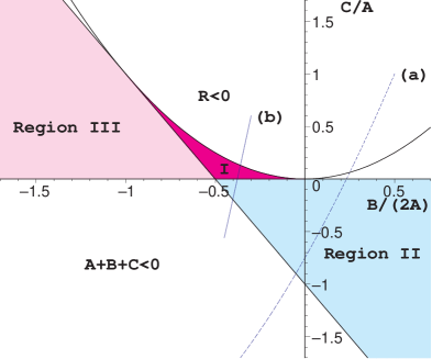
Line segment (a) corresponds to the integration region of a triangle function where only logarithmic singularities are present, while for line segment (b) square-root and logarithmic singularities are present. Note that the box function has the same singularity structure. As and are the basic building blocks, this analysis of the singularity structure is done once and for all.
24.4.4 Numerical integration
We now discuss the numerical evaluation of the analytic expressions derived above.414141A more detailed description can be found in Ref. [303]. So far, we showed that any finite scalar -point function can be written as a linear combination of the basic building block of Eq. (73) and a similar 2-dimensional integral, , with coefficients that are rational functions of the kinematical invariants and masses. To avoid numerical instabilities, the residual dimensions of and are then integrated over numerically. Since scalar function expressions can contain dozens of building blocks and an amplitude has to be evaluated many times to calculate a cross section, a fast method to evaluate the basic building blocks is called for. However, the naive application of standard numerical integration techniques is not sufficient to achieve this objective. This is due to the presence of integrable singularities and step discontinuities in the integrands, which the detailed analysis above revealed. It prevents the naive application of deterministic, integration-rule based algorithms that are better suited for fast evaluation than the more robust, but significantly slower Monte Carlo techniques commonly used to evaluate multi-particle cross sections in high energy physics.
Several approaches can be pursued to achieve a sufficiently fast and accurate numerical integration of the basic building blocks. A first direction are automatic methods, i.e. methods that do not require knowledge of the exact location and type of the discontinuities. The key to success here are adaptive algorithms that iteratively divide the integration volume into non-uniform subvolumes and apply basic numerical integration methods to each subvolume until an optimal partition of the integration volume minimizes the total error. Using this approach the 1-dimensional integral of can be integrated with negligible time requirements (fractions of a second). The 2-dimensional integral of is much more challenging, but can be tackled in the same spirit by combining deterministic and Monte Carlo integration techniques (see Ref. [304] and references therein). We note that the time required to integrate all building blocks of the scalar hexagon function using this approach depends on the kinematical configuration and, while sufficiently short at this stage, is no longer negligible. If, at a subsequent stage, i.e. for the calculation of a certain cross section, the building blocks had to be computed in a time comparable to the one for the functions, a second direction could be pursued. Since the location of all singularities and step discontinuities is known analytically, one can identify regions with continuous integrand and in each region flatten the integrand either by transforming integration variables or subtracting singular approximations. The resulting bounded integrands could then be integrated numerically with standard deterministic methods at a speed that would facilitate millions of amplitude evaluations in a reasonable amount of time.
To demonstrate the practicality of our method to evaluate multi-leg integrals, we show in Fig. 58 a scan of the GeV threshold of the 4-dimensional scalar hexagon function for a kinematical configuration appropriate for the Feynman diagram to the right in Fig. 56.
24.5 Conclusion
We have outlined new algebraic/numerical approaches for 1-loop calculations. We have shown that our algebraic formalism leads to compact representations of complicated 1-loop amplitudes. Furthermore we have constructed numerical methods for general hexagon kinematics. The presented methods are parts of a project to describe multi-particle/jet production at TeV colliders with kinematics at the 1-loop level.
Acknowledgements
We would like to thank the conference organizers! This research has been supported by the Bundesministerium für Bildung und Forschung (BMBF, Bonn, Germany) under the contract under the contract number 05HT1WWA2.
25 INFRARED DIVERGENCES AT NNLO 424242Contributed by: G. Heinrich, S. Weinzierl
25.1 Introduction
Fully differential NNLO calculations are needed to increase the accuracy of theoretical predictions and are relevant to high-energy collider experiments, in particular for the Tevatron and the LHC. They involve a variety of technical complications, such as the calculation of two-loop amplitudes, a method for the cancellation of infrared divergences and stable and efficient numerical methods for the final computer program. There has been a significant progress in the calculation of two-loop amplitudes in the past years [305, 306, 307, 308, 309, 310, 311, 312, 313, 314, 315, 316, 317]. Here we review the state of the art for the cancellation of infrared divergences at NNLO.
Infrared divergences occur already at next-to-leading order. At NLO real and virtual corrections contribute. The virtual corrections contain the loop integrals and can have, in addition to ultraviolet divergences, infrared divergences. If loop amplitudes are calculated in dimensional regularisation, the IR divergences manifest themselves as explicit poles in the dimensional regularisation parameter . These poles cancel with similar poles arising from amplitudes with additional partons but less internal loops, when integrated over phase space regions where two (or more) partons become “close” to each other. In general, the Kinoshita-Lee-Nauenberg theorem [318, 319] guarantees that any infrared-safe observable, when summed over all states degenerate according to some resolution criteria, will be finite. However, the cancellation occurs only after the integration over the unresolved phase space has been performed and prevents thus a naive Monte Carlo approach for a fully exclusive calculation. It is therefore necessary to cancel first analytically all infrared divergences and to use Monte Carlo methods only after this step has been performed.
At NLO, general methods to circumvent this problem are known. This is possible due to the universality of the singular behaviour of the amplitudes in soft and collinear limits. Examples are the phase-space slicing method [295, 281, 296] and the subtraction method [320, 269, 321, 298, 299]. It is worth to examine a simple NLO example in detail to understand the basic concepts which are currently under discussion for an extension to NNLO. We consider the NLO corrections to The real corrections are given by the matrix element for and read, up to colour and coupling factors
| (74) |
where and . This term is integrated over the three particle phase space
| (75) |
Singularities occur at the boundaries of the integration region at and . Historically, phase space slicing [295, 281, 296] has been the first systematic method to treat the infrared singularities. Here, one splits the integration region into different parts, shown in fig. 59: A soft region, given by and , two collinear regions, corresponding to and and a hard region region . The hard region is free of singularities and the integration can be performed numerically there. In the remaining regions the matrix element is approximated by the soft or collinear factorisation formulae and the integration over a one-parton phase space can then be performed analytically. Phase space slicing has the advantage, that different factorisation formulae may be used in different regions of phase space. However, there are also some disadvantages: The method introduces a systematic error of order , it becomes rather intricate for colour-subleading terms and it poses a numerical problem: The hard region gives a contribution of the form
| (76) |
The logarithms and cancel against the contributions from the other regions, but this cancelation happens only numerically.
Within the subtraction method [320, 269, 321, 298, 299] one subtracts a suitable approximation term from the real corrections . This approximation term must have the same singularity structure as the real corrections. If in addition the approximation term is simple enough, such that it can be integrated analytically over a one-parton subspace, then the result can be added back to the virtual corrections .
| (77) |
Since by definition has the same singular behaviour as , acts as a local counter-term and the combination is integrable and can be evaluated numerically. Secondly, the analytic integration of over the one-parton subspace will yield the explicit poles in needed to cancel the corresponding poles in . The subtraction method overcomes the short-comings of the slicing method, but there is a price to pay: The approximation term is subtracted over the complete phase space and has to interpolate between different singular regions. At NLO this requires an interpolation between soft and collinear regions. For the example discussed above the approximation term can be taken as a sum of two (dipole) subtraction terms:
| (78) | |||||
The momenta , , and are linear combinations of the original momenta , and . The first term is an approximation for , whereas the second term is an approximation for . Note that the soft singularity is shared between the two dipole terms and that in general the Born amplitudes are evaluated with different momenta. The subtraction terms can be derived by working in the axial gauge. In this gauge only diagrams where the emission occurs from external lines are relevant for the subtraction terms. Alternatively, they can be obtained from off-shell currents. Antenna factorisation [322, 323, 324, 325] allows to reduce the number of subtraction terms needed and interpolates smoothly between the and regions.
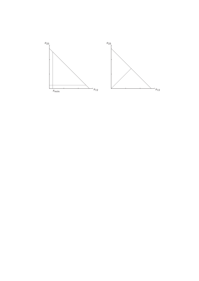
We briefly sketch how to obtain the antenna function from off-shell currents. The amplitude for is constructed from the quark and antiquark currents and as follows:
| (79) |
is the polarisation vector of the photon, contracted into the Dirac matrix . Singular contributions can only arise from the currents and . With a suitable pair of reconstruction functions and one achieves that the Born amplitude is evaluated with the same set of momenta and one can approximate the amplitude by
| (80) |
Note that in general the momenta and are non-linear functions of the original momenta , and .
Once suitable subtraction terms are found, they have to be integrated over the unresolved phase space. Here, one faces integrals with overlapping divergences, as one can already see from our simple example:
| (81) |
The term is an overlapping singularity. Sector decomposition [326, 327, 328] is a convenient tool to disentangle overlapping singularities. Here one splits the integration region into two sectors and , as shown in fig. 59. In the fist sector one rescales as , while in the second sector one rescales . Sector decomposition is discussed in detail in sect. 25.3.
25.2 The subtraction method at NNLO
The following terms contribute at NNLO:
| (82) |
where denotes an amplitude with external partons and loops. is the phase space measure for partons. Taken separately, each of these contributions is divergent. Only the sum of all contributions is finite. We would like to construct a numerical program for an arbitrary infrared safe observable . Infrared safety implies that whenever a parton configuration ,…, becomes kinematically degenerate with a parton configuration ,…, we must have
| (83) |
To render the individual contributions finite, one adds and subtracts suitable pieces [329, 330]:
| (84) | |||||
Here is a subtraction term for single unresolved configurations of Born amplitudes. This term is already known from NLO calculations. The term is a subtraction term for double unresolved configurations. Finally, is a subtraction term for single unresolved configurations involving one-loop amplitudes.
To construct these terms the universal factorisation properties of QCD amplitudes in unresolved limits are essential. QCD amplitudes factorise if they are decomposed into primitive amplitudes. Primitive amplitudes are defined by a fixed cyclic ordering of the QCD partons, a definite routing of the external fermion lines through the diagram and the particle content circulating in the loop. One-loop amplitudes factorise in single unresolved limits as [331, 332, 333, 334, 335, 336, 324]
| (85) |
Tree amplitudes factorise in the double unresolved limits as [337, 338, 339, 340, 341, 342, 323]
| (86) |
To discuss the term let us consider as an example the Born leading-colour contributions to , which contribute to the NNLO corrections to . The subtraction term has to match all double and single unresolved configurations. It is convenient to construct as a sum over several pieces,
| (87) |
Each piece is labelled by a splitting topology.

An example is shown in fig. 60. The term corresponding to the topology shown in fig. 60 approximates singularities in , and part of the singularities in . Care has to be taken to disentangle correctly overlapping singularities like . Details can be found in [329].
25.2.1 One-loop amplitudes with one unresolved parton
Apart from also the term , which approximates one-loop amplitudes with one unresolved parton, is needed at NNLO. If we recall the factorisation formula (85), this requires as a new feature the approximation of the one-loop singular function . The corresponding subtraction term is proportional to the one-loop splitting function . An example is the leading-colour part for the splitting [330]:
| (88) | |||||
This term depends on the correlations among the remaining hard partons. If only two hard partons are correlated, is given by
| (89) | |||||
Here, , and . The parameter specifies the variant of dimensional regularisation: in the conventional or ’t Hooft-Veltman scheme and in a four-dimensional scheme. For the integration of the subtraction terms over the unresolved phase space all occuring integrals are reduced to standard integrals of the form
The result is proportional to hyper-geometric functions with unit argument and can be expanded into a Laurent series in with the techniques of [343, 344]. For the example discussed above one finds after integration [330]:
| (91) | |||||
where .
25.3 Isolation of infrared poles by sector decomposition
As is well known, for ultraviolet divergences a general subtraction scheme to all orders can be established [345, 326, 346]. For infrared poles, i.e. soft and collinear poles in Minkowski space, the situation is less settled. Of course, general cancellation theorems like the KLN theorem [318, 319] exist, but a local subtraction scheme acting on a graph by graph basis and being valid to all orders is not available.
On the other hand, the use of dimensional regularisation in combination with Feynman (or alpha [347]) parameters allows in principle to isolate the infrared poles as powers in for an arbitrary graph. The problem is that the corresponding parameter integrals get extremely complicated the more loops and scales are involved, in particular they exhibit an overlapping structure. A simple example of an overlapping singularity already has been given in eq. (81).
To address this problem, an automated algorithm434343The method of sector decomposition has been used first in [326] for overlapping UV divergences, and applied in a different context in [327]. presented in [328] and sketched below has been constructed which disentangles the overlapping regions in parameter space by decomposing them iteratively into subsectors until the divergent contributions factorise. Arrived at the factorised form, subtractions can be implemented easily. The resulting parameter integrals for the pole coefficients are in general too complicated to be integrated analytically, but as they are finite, they can be integrated numerically.
25.3.1 Multi-loop integrals
The straightforward automatisation of the algorithm is one of its virtues, and this is in particular true when applied to virtual loop integrals, because the latter, after Feynman parametrisation, have a ”standard form”: An -loop graph in dimensions with propagators is, after momentum integration, of the form
| (92) |
The functions and can be straightforwardly derived from the momentum representation, or they can be constructed from the topology of the corresponding Feynman graph [348, 347]. is a polynomial of degree in the Feynman parameters, is of degree and also depends on the kinematic invariants of the diagram. The sector decomposition uses representation (92) as a starting point and proceeds as follows:
-
The integration domain is split into parts, using the identity
(93) such that becomes a sum over integrals , where in each ”primary sector” the variable is the largest one.
-
The variables are transformed in each primary sector as follows:
(95) -
By construction, factorises from and . We eliminate in each using
By applying the sector decomposition iteratively, one finally arrives at a form where all singularities are factorised explicitly in terms of factors of Feynman parameters like . Subtractions of the form
for each , where is finite by construction, and subsequent expansion in leads to a representation of the graph as a Laurent series in :
| (96) |
The pole coefficients are sums of integrals over functions of Feynman parameters. Of course they also contain the kinematic invariants defined by the graph. For the numerical integration of those functions, two cases can be distinguished: If the diagrams depend only on a single scale, this scale can be factored out and the pole coefficients are just numbers which can be calculated once and for all. For diagrams depending on several scales, like for example the Mandelstam variables and in the case of the massless -loop box, the kinematic invariants have to be fixed to certain values at which the diagram is evaluated. These have to be in the Euclidean region in order to avoid that thresholds spoil the numerical integration.
As an example for a one-scale problem, we give the result for a five-loop propagator diagram, shown in Fig. 61.
Examples of diagrams depending on four scales are given in Fig. 62, where the two straight lines flowing through the graphs denote massive propagators which can have different masses.
These graphs are the most complicated ones occurring in the calculation of two-loop Bhabha scattering. Only topology , for the case of one single mass scale, has been calculated analytically so far by Smirnov [349]. A calculation of all three graphs only exists in the massless approximation [305]. Our numerical results at two different points for are given in Table 6.
| -1.561 | -0.5255 | -1.152 | -0.08622 | -0.03483 | -0.05832 | |
| -5.335 | -0.2024 | -3.690 | -0.04195 | 0.07556 | 0.05389 | |
| 1.421 | 3.606 | 1.555 | 0.7323 | 0.1073 | 0.6847 | |
25.3.2 Phase space integrals
As already explained in detail above, solving the problem of isolating and subtracting the infrared poles occurring in NNLO phase space integrals, and of integrating over the divergent subtraction terms, is a major step towards a (partonic) Monte Carlo program calculating processes like for example or 3 jets at NNLO. The method of sector decomposition can also be very useful for this task, as it is a general method to isolate (overlapping) poles in parameter space. Its first application to phase space integrals can be found in [350], further developments of the method will be sketched in the following.
In order to be able to use the automated sector decomposition procedure for phase space integrals, the phase space has to be cast into a ”standard form”, similar to (92) for loop integrals. For example, a parton phase space is most conveniently written as
where the parameters are rescaled Mandelstam invariants, defined by
and
is the Källen function,
.
In order to calculate the real emission part where up to two particles can be unresolved using the method of sector decomposition, there are several ways to go, ranging from the use of this method only as a check for integrals over subtraction terms calculated analytically to an almost completely numerical approach relying largely on this method. The former has been employed in [351], where it has been shown that any term appearing in a phase space integral of a matrix element in massless QCD can be expressed as a linear combination of only four master integrals, where one of them is the ”trivial” integral over the phase space alone. In the notation introduced above, the remaining three master integrals are
| (97) | |||||
| (98) | |||||
| (99) |
Their analytical evaluation could be achieved by calculating explicitly and deriving the others from unitarity relations involving known results for three-loop two-point functions. The numerical results obtained by the sector decomposition algorithm,
agree with the analytical results within a numerical precision better than 1%.
The algorithm can also be employed to avoid complicated analytical integrations over subtraction terms completely. The singularities can be extracted as outlined above, and the pole coefficients can be calculated numerically to a high precision to check their cancellation against the double virtual respectively one-loop virtual plus single-real-emission counterparts. The remaining functions are finite, and the combination with an arbitrary (infrared safe) measurement function is straightforward as it does not hamper the numerical integration. In this way, fully differential Monte Carlo programs for particle/jet processes can be constructed. A first step in this direction already has been undertaken in [352], where the contribution proportional to of or 4 jets has been calculated using sector decomposition techniques.
Certainly, the automated sector decomposition algorithm applied to phase space integrals can also be useful in cases where massive particles are involved. As has been already proven by explicit examples in the case of loop integrals [353], masses do not present a principle problem for the method, but of course care has to be taken that thresholds do not destroy the numerical stability.
Acknowledgements
We would like to thank the conference organisers for a stimulating and productive workshop.
References
- [1] T. Sjöstrand and M. van Zijl, Phys. Rev. D36 (1987) 2019.
- [2] B. Andersson, G. Gustafson, G. Ingelman, and T. Sjostrand, Phys. Rept. 97 (1983) 31.
- [3] R.D. Field. See talks available from http://www.phys.ufl.edu/rfield/cdf/.
- [4] T. Sjöstrand and P. Skands, Nucl. Phys. B659 (2003) 243, [hep-ph/0212264].
- [5] T. Sjöstrand and P. Skands, hep-ph/0402078.
- [6] J. Dischler and T. Sjostrand, Eur. Phys. J. direct C3 (2001) 2, [hep-ph/0011282].
- [7] T. Sjöstrand, L. Lönnblad, S. Mrenna, and P. Skands, hep-ph/0308153.
- [8] P. D. B. Collins and A. D. Martin, Rep. Prog. Phys. 45 (1982) 335.
- [9] A. Capella et. al., Phys. Rep. 236 (1994) 225.
- [10] T. Sjostrand et. al., Comput. Phys. Commun. 135 (2001) 238–259, [hep-ph/0010017].
- [11] T. Sjostrand, L. Lonnblad, and S. Mrenna, hep-ph/0108264. PYTHIA 6.2 - Physics and Manual.
- [12] R. Engel, Z. Phys. C66 (1995) 203.
- [13] R. Engel, PHOJET manual (program version 1.05).
- [14] Engel, R. Hadronic Interactions of Photons at High Energies. Ph.D. thesis, University of Siegen, 1997.
- [15] A. Breakstone et. al., Phys. Rev. D30 (1984) 528.
- [16] G. J. Alner et. al., Phys. Rept. 154 (1987) 247–383.
- [17] F. Abe et. al., Phys. Rev. D41 (1990) 2330.
- [18] T. Alexopoulos et. al., Phys. Lett. B435 (1998) 453–457.
- [19] S. G. Matinyan and W. D. Walker, Phys. Rev. D59 (1999) 034022, [hep-ph/9801219].
- [20] Z. Koba, H. B. Nielsen, and P. Olesen, Nucl. Phys. B40 (1972) 317–334.
- [21] R. E. Ansorge et. al., Z. Phys. C43 (1989) 357.
- [22] T. Affolder et. al., Phys. Rev. D65 (2002) 092002.
- [23] T. Sjöstrand, Phys. Lett. B157 (1985) 321.
- [24] M. Bengtsson, T. Sjöstrand, and M. van Zijl, Z. Phys. C32 (1986) 67.
- [25] J. Huston, A Comparison of the Underlying Event in Jet and Min-Bias Events. Talk presented at DPF2000, Columbus, OH, August 11, 2000.
- [26] V. Tano, The Underlying Event in Jet and Minimum Bias Events at the Tevatron. Talk presented at ISMD2001, Datong, China, September 1–7, 2001.
- [27] R.D. Field, Min-Bias and the Underlying Event at the Tevatron and the LHC. Talk presented at the Fermilab ME/MC Tuning Workshop, Fermilab, October 4, 2002.
- [28] R.D. Field, Toward an Understanding of Hadron Collisions: From Feynman-Field until Now. Talk presented at the Fermilab Joint Theoretical Experimental Seminar, Fermilab, October 4, 2002.
- [29] R.D. Field, Min-Bias and the Underlying Event at CDF. Talk presented at the Monte-Carlo Tools for the LHC Workshop, CERN, July 31, 2003.
- [30] G. Marchesini and B. R. Webber, Nucl. Phys. B310 (1988) 461.
- [31] I. G. Knowles, Nucl. Phys. B310 (1988) 571.
- [32] S. Catani, B. R. Webber, and G. Marchesini, Nucl. Phys. B349 (1991) 635–654.
- [33] D. Acosta et. al., Phys. Rev. D65 (2002) 072005.
- [34] CDF II Collaboration FERMILAB 390-E (1996).
- [35] M. L. Mangano, M. Moretti, F. Piccinini, R. Pittau, and A. D. Polosa, JHEP 0307:001 (2003) 35, [hep-ph/0206293].
-
[36]
V. Ilyin, PEVLIB,
/afs/cern.ch/cms/physics/PEVLIB/. - [37] A. Pukhov et. al., hep-ph/9908288.
-
[38]
http://www.fnal.gov/docs/products/enstore/enstoreTOC.html. -
[39]
L. Dudko and S. Mrenna, FNAL MCDB,
http://www-d0.fnal.gov/~dudko/mcdb. -
[40]
L. Dudko and A. Sherstnev, CMS MCDB,
http://cmsdoc.cern.ch/cms/generators/mcdb. -
[41]
L. Dudko and A. Sherstnev, CMS MCDB: direct AFS link,
/afs/cern.ch/cms/generators/{mcdb,mcdb2,mcdb3}. - [42] P. Bartalini, L. Dudko, A. Kryukov, I. Seluzhenkov, A. Sherstnev, and A. Vologdin, LCG Monte-Carlo Data Base, LCG note, in preparation.
- [43] C. Balazs, J. Huston, and I. Puljak, Phys. Rev. D63 (2001) 014021, [hep-ph/0002032].
- [44] J. Collins and D. Soper, Nucl. Phys. B193 (1981) 381.
- [45] G. Miu and T. Sjöstrand, Phys. Lett. B449 (1999) 313–320, [hep-ph/9812455].
- [46] E. Thomé, hep-ph/0401121.
- [47] H. L. Lai et. al.,, CTEQ Collaboration Eur. Phys. J. C12 (2000) 375–392, [hep-ph/9903282].
- [48] T. Sjöstrand, these proceedings.
- [49] T. Affolder et. al.,, CDF Collaboration Phys. Rev. Lett. 84 (2000) 845–850, [hep-ex/0001021].
- [50] C. Balazs et. al., these proceedings.
- [51] G. Bozzi, S. Catani, D. de Florian, and M. Grazzini, Phys. Lett. B564 (2003) 65–72, [hep-ph/0302104].
- [52] C. Balazs and C. P. Yuan, Phys. Lett. B478 (2000) 192–198, [hep-ph/0001103].
- [53] A. Kulesza, G. Sterman, and W. Vogelsang, Phys. Rev. D69 (2004) 014012, [hep-ph/0309264].
- [54] E. Berger and J. Qiu, Phys. Rev. D67 (2003) 034026, [hep-ph/0210135].
- [55] S. Frixione and B. Webber, JHEP 06 (2002) 029, [hep-ph/0204244].
- [56] S. Frixione, P. Nason, and B. Webber, JHEP 08 (2003) 007, [hep-ph/0305252].
- [57] G. Corcella et. al., JHEP 01 (2001) 010, [hep-ph/0011363].
- [58] M. Bengtsson and T. Sjöstrand, Nucl. Phys. B289 (1987) 810.
- [59] E. Norrbin and T. Sjöstrand, Nucl. Phys. B603 (2001) 297–342, [hep-ph/0010012].
- [60] G. Marchesini and B. Webber, Nucl. Phys. B238 (1984) 1.
- [61] L. Lönnblad, Comput. Phys. Commun. 71 (1992) 15–31.
- [62] H. Kharraziha and L. Lönnblad, JHEP 03 (1998) 006, [hep-ph/9709424].
- [63] S. Catani, F. Krauss, R. Kuhn, and B. R. Webber, JHEP 11 (2001) 063, [hep-ph/0109231].
- [64] L. Lönnblad, JHEP 05 (2002) 046, [hep-ph/0112284].
- [65] T. Sjöstrand and P. Skands, these proceedings.
- [66] S. Moretti, L. Lönnblad, and T. Sjöstrand, JHEP 08 (1998) 001, [hep-ph/9804296].
- [67] J. Huston, I. Puljak, T. Sjöstrand, and E. Thomé, these proceedings.
- [68] T. Sjostrand and M. Bengtsson, Comput. Phys. Commun. 43 (1987) 367.
- [69] M. Bengtsson and T. Sjostrand, Z. Phys. C37 (1988) 465.
- [70] G. Corcella et. al., hep-ph/0210213.
- [71] M. H. Seymour, Z. Phys. C56 (1992) 161–170.
- [72] M. H. Seymour, contributed to 27th International Conference on High Energy Physics (ICHEP), Glasgow, Scotland, 20-27 Jul 1994.
- [73] G. Corcella and M. H. Seymour, Phys. Lett. B442 (1998) 417–426, [hep-ph/9809451].
- [74] G. Corcella and M. H. Seymour, Nucl. Phys. B565 (2000) 227–244, [hep-ph/9908388].
- [75] M. H. Seymour, Comp. Phys. Commun. 90 (1995) 95–101, [hep-ph/9410414].
- [76] F. Krauss, JHEP 08 (2002) 015, [hep-ph/0205283].
- [77] F. Maltoni and T. Stelzer, hep-ph/0208156.
- [78] E. Boos et. al., hep-ph/0109068.
- [79] N. Kidonakis and G. Sterman, Phys. Lett. B387 (1996) 867.
- [80] N. Kidonakis and G. Sterman, Nucl. Phys. B505 (1997) 321, [hep-ph/9705234].
- [81] N. Kidonakis, G. Oderda, and G. Sterman, Nucl. Phys. B531 (1998) 365, [hep-ph/9803241].
- [82] N. Kidonakis, Int. J. Mod. Phys. A15 (2000) 1245, [hep-ph/9902484].
- [83] N. Kidonakis, hep-ph/0303186.
- [84] P. B. Arnold and M. H. Reno, Nucl. Phys. B319 (1989) 37.
- [85] R. J. Gonsalves, J. Pawlowski, and C.-F. Wai, Phys. Rev. D40 (1989) 2245.
- [86] R. J. Gonsalves, J. Pawlowski, and C.-F. Wai, Phys. Lett. B252 (1990) 663.
- [87] N. Kidonakis and V. Del Duca, Phys. Lett. B480 (2000) 87, [hep-ph/9911460].
- [88] N. Kidonakis and A. Sabio Vera, JHEP 02 (2004) 027, [hep-ph/0311266].
- [89] A. D. Martin, R. G. Roberts, W. J. Stirling, and R. S. Thorne, Eur. Phys. J. C28 (2003) 455, [hep-ph/0211080].
- [90] P. Aurenche, A. Douiri, R. Baier, M. Fontannaz, and D. Schiff, Phys. Lett. B140 (1984) 87.
- [91] P. Aurenche, R. Baier, M. Fontannaz, and D. Schiff, Nucl. Phys. B297 (1988) 661.
- [92] L. E. Gordon and W. Vogelsang, Phys. Rev. D48 (1993) 3136.
- [93] N. Kidonakis and J. F. Owens, Phys. Rev. D61 (2000) 094004, [hep-ph/9912388].
- [94] N. Kidonakis and J. F. Owens, Int. J. Mod. Phys. A19 (2004) 149, [hep-ph/0307352].
- [95] H. Baer, J. Ohnemus, and J. F. Owens, Phys. Rev. D42 (1990) 61.
- [96] B. W. Harris and J. F. Owens, Phys. Rev. D65 (2002) 094032, [hep-ph/0102128].
- [97] L. Bourhis, M. Fontannaz, J. P. Guillet, and M. Werlen, Eur. Phys. J. C19 (2001) 89, [hep-ph/0009101].
- [98] J. Pumplin et. al., JHEP 07 (2002) 012, [hep-ph/0201195].
- [99] L. Apanasevich et. al., Phys. Rev. Lett. 81 (1998) 2642, [hep-ex/9711017].
- [100] G. Ballocchi et. al.,, UA6 Collaboration Phys. Lett. B436 (1998) 222.
- [101] N. Kidonakis, Phys. Rev. D64 (2001) 014009, [hep-ph/0010002].
- [102] N. Kidonakis, E. Laenen, S. Moch, and R. Vogt, Phys. Rev. D64 (2001) 114001, [hep-ph/0105041].
- [103] N. Kidonakis and R. Vogt, Phys. Rev. D68 (2003) 114014, [hep-ph/0308222].
- [104] N. Kidonakis and A. Belyaev, JHEP 12 (2003) 004, [hep-ph/0310299].
- [105] G. Sterman, Nucl. Phys. B281 (1987) 310.
- [106] S. Catani and L. Trentadue, Nucl. Phys. B327 (1989) 323.
- [107] M. Kramer, E. Laenen, and M. Spira, Nucl. Phys. B511 (1998) 523–549, [hep-ph/9611272].
- [108] G. Parisi, Phys. Lett. B90 (1980) 295.
- [109] L. Magnea and G. Sterman, Phys. Rev. D42 (1990) 4222–4227.
- [110] H. Contopanagos, E. Laenen, and G. Sterman, Nucl. Phys. B484 (1997) 303–330, [hep-ph/9604313].
- [111] R. Akhoury, M. Sotiropoulos, and G. Sterman, Phys. Rev. Lett. 81 (1998) 3819–3822, [hep-ph/9807330].
- [112] R. Akhoury and M. Sotiropoulos, hep-ph/0304131.
- [113] Y. Dokshitzer, private communication.
- [114] E. Laenen, G. Sterman, and W. Vogelsang, Phys. Rev. D63 (2001) 114018, [hep-ph/0010080].
- [115] T. Eynck, E. Laenen, and L. Magnea, JHEP 06 (2003) 057, [hep-ph/0305179].
- [116] E. Gardi and R. Roberts, Nucl. Phys. B653 (2003) 227–255, [hep-ph/0210429].
- [117] W. van Neerven and E. Zijlstra, Nucl. Phys. B382 (1992) 11–62.
- [118] H.-n. Li, Phys. Lett. B454 (1999) 328–334, [hep-ph/9812363].
- [119] A. Kulesza, G. Sterman, and W. Vogelsang, Phys. Rev. D66 (2002) 014011, [hep-ph/0202251].
- [120] E. Laenen, G. Sterman, and W. Vogelsang, Phys. Rev. Lett. 84 (2000) 4296–4299, [hep-ph/0002078].
- [121] A. Banfi and E. Laenen, in preparation.
- [122] D. Cavalli et. al., hep-ph/0203056.
- [123] S. Catani, D. de Florian, and M. Grazzini, JHEP 05 (2001) 025, [hep-ph/0102227].
- [124] R. Harlander and W. Kilgore, Phys. Rev. D64 (2001) 013015, [hep-ph/0102241].
- [125] R. Harlander and W. Kilgore, Phys. Rev. Lett. 88 (2002) 201801, [hep-ph/0201206].
- [126] C. Anastasiou and K. Melnikov, Nucl. Phys. B646 (2002) 220–256, [hep-ph/0207004].
- [127] V. Ravindran, J. Smith, and W. L. van Neerven, Nucl. Phys. B665 (2003) 325–366, [hep-ph/0302135].
- [128] S. Catani, D. de Florian, M. Grazzini, and P. Nason, JHEP 07 (2003) 028, [hep-ph/0306211].
- [129] G. Parisi and R. Petronzio, Nucl. Phys. B154 (1979) 427.
- [130] Y. Dokshitzer, D. Diakonov, and S. I. Troian, Phys. Rept. 58 (1980) 269–395.
- [131] J. C. Collins, D. E. Soper, and G. Sterman, Nucl. Phys. B250 (1985) 199.
- [132] S. Catani, D. de Florian, and M. Grazzini, Nucl. Phys. B596 (2001) 299, [hep-ph/0008184].
- [133] S. Catani, E. D’Emilio, and L. Trentadue, Phys. Lett. B211 (1988) 335.
- [134] W. Giele et. al., hep-ph/0204316.
- [135] R. P. Kauffman, Phys. Rev. D45 (1992) 1512–1517.
- [136] D. de Florian and M. Grazzini, Phys. Rev. Lett. 85 (2000) 4678, [hep-ph/0008152].
- [137] D. de Florian and M. Grazzini, Nucl. Phys. B616 (2001) 247–285, [hep-ph/0108273].
- [138] A. Vogt, Phys. Lett. B497 (2001) 228–234, [hep-ph/0010146].
- [139] S. Catani et. al., hep-ph/0005114.
- [140] C. Balazs and C. P. Yuan, Phys. Rev. D56 (1997) 5558–5583, [hep-ph/9704258].
- [141] G. Corcella and S. Moretti, hep-ph/0402146.
- [142] D. de Florian, M. Grazzini, and Z. Kunszt, Phys. Rev. Lett. 82 (1999) 5209–5212, [hep-ph/9902483].
- [143] Z. Kunszt, S. Moretti, and W. J. Stirling, Z. Phys. C74 (1997) 479–491, [hep-ph/9611397].
- [144] A. Djouadi et. al., hep-ph/0002258.
- [145] M. Dobbs, Phys. Rev. D64 (2001) 034016, [hep-ph/0103174].
- [146] U. Baur and E. W. N. Glover, Nucl. Phys. B339 (1990) 38–66.
- [147] S. Moretti, K. Odagiri, P. Richardson, M. H. Seymour, and B. R. Webber, JHEP 04 (2002) 028, [hep-ph/0204123].
- [148] S. Frixione and B. Webber, hep-ph/0309186.
- [149] S. Bethke, J. Phys. G26 (2000) R27, [hep-ex/0004021].
- [150] R. W. L. Jones, M. Ford, G. P. Salam, H. Stenzel, and D. Wicke, JHEP 12 (2003) 007, [hep-ph/0312016].
- [151] S. Kluth, P. A. Movilla Fernandez, S. Bethke, C. Pahl, and P. Pfeifenschneider, Eur. Phys. J. C21 (2001) 199–210, [hep-ex/0012044].
- [152] M. Dasgupta and G. P. Salam, hep-ph/0312283.
- [153] S. Catani, L. Trentadue, G. Turnock, and B. R. Webber, Nucl. Phys. B407 (1993) 3–42.
- [154] A. Banfi, G. P. Salam, and G. Zanderighi, hep-ph/0304148.
- [155] N. Brown and W. J. Stirling, Phys. Lett. B252 (1990) 657–662.
- [156] M. Dasgupta and G. P. Salam, Phys. Lett. B512 (2001) 323–330, [hep-ph/0104277].
- [157] A. Banfi, G. P. Salam, and G. Zanderighi, JHEP 01 (2002) 018, [hep-ph/0112156].
- [158] S. Haywood et. al., hep-ph/0003275.
- [159] ATLAS detector and physics performance. Technical design report. Vol. 2. CERN-LHCC-99-15.
- [160] U. Baur, R.K. Ellis and D. Zeppenfeld, eds. Proceedings of Physics at Run II: QCD and Weak Boson Physics Workshop, Batavia, Illinois, 1999.
- [161] C. Balazs, J.-w. Qiu, and C. P. Yuan, Phys. Lett. B355 (1995) 548–554, [hep-ph/9505203].
- [162] T. Affolder et. al.,, CDF Collaboration Phys. Rev. D64 (2001) 052001, [hep-ex/0007044].
- [163] S. Dittmaier and M. Kramer, Phys. Rev. D65 (2002) 073007, [hep-ph/0109062].
- [164] U. Baur, S. Keller, and D. Wackeroth, Phys. Rev. D59 (1999) 013002, [hep-ph/9807417].
- [165] Q.-H. Cao and C.-P. Yuan, hep-ph/0401026.
- [166] P. Nadolsky, D. R. Stump, and C. P. Yuan, Phys. Rev. D61 (2000) 014003, [hep-ph/9906280].
- [167] P. M. Nadolsky, D. R. Stump, and C. P. Yuan, Phys. Rev. D64 (2001) 114011, [hep-ph/0012261].
- [168] E. A. Kuraev, L. N. Lipatov, and V. S. Fadin, Sov. Phys. JETP 44 (1976) 443–450.
- [169] I. I. Balitsky and L. N. Lipatov, Sov. J. Nucl. Phys. 28 (1978) 822–829.
- [170] F. Landry, R. Brock, P. M. Nadolsky, and C. P. Yuan, Phys. Rev. D67 (2003) 073016, [hep-ph/0212159].
- [171] D. Stump et. al., JHEP 10 (2003) 046, [hep-ph/0303013].
- [172] J. Kodaira and L. Trentadue, Phys. Lett. B112 (1982) 66.
- [173] C. T. H. Davies and W. J. Stirling, Nucl. Phys. B244 (1984) 337.
- [174] R. P. Kauffman, Phys. Rev. D44 (1991) 1415.
- [175] C. P. Yuan, Phys. Lett. B283 (1992) 395.
- [176] Z. Bern, L. J. Dixon, and C. Schmidt, Phys. Rev. D66 (2002) 074018, [hep-ph/0206194].
- [177] L. N. Lipatov, Sov. J. Nucl. Phys. 23 (1976) 338–345.
- [178] V. S. Fadin, E. A. Kuraev, and L. N. Lipatov, Phys. Lett. B60 (1975) 50–52.
- [179] E. A. Kuraev, L. N. Lipatov, and V. S. Fadin, Sov. Phys. JETP 45 (1977) 199–204.
- [180] I. I. Balitsky and L. N. Lipatov, JETP Lett. 30 (1979) 355.
- [181] V. S. Fadin and L. N. Lipatov, Phys. Lett. B429 (1998) 127–134, [hep-ph/9802290].
- [182] M. Ciafaloni and G. Camici, Phys. Lett. B430 (1998) 349–354, [hep-ph/9803389].
- [183] D. A. Ross, Phys. Lett. B431 (1998) 161–165, [hep-ph/9804332].
- [184] E. Levin, hep-ph/9806228.
- [185] G. P. Salam, JHEP 07 (1998) 019, [hep-ph/9806482].
- [186] M. Ciafaloni and D. Colferai, Phys. Lett. B452 (1999) 372–378, [hep-ph/9812366].
- [187] S. J. Brodsky, V. S. Fadin, V. T. Kim, L. N. Lipatov, and G. B. Pivovarov, JETP Lett. 70 (1999) 155–160, [hep-ph/9901229].
- [188] C. R. Schmidt, Phys. Rev. D60 (1999) 074003, [hep-ph/9901397].
- [189] J. R. Forshaw, D. A. Ross, and A. Sabio Vera, Phys. Lett. B455 (1999) 273–282, [hep-ph/9903390].
- [190] M. Ciafaloni, D. Colferai, and G. P. Salam, Phys. Rev. D60 (1999) 114036, [hep-ph/9905566].
- [191] R. D. Ball and S. Forte, Phys. Lett. B465 (1999) 271–281, [hep-ph/9906222].
- [192] G. Altarelli, R. D. Ball, and S. Forte, Nucl. Phys. B575 (2000) 313–329, [hep-ph/9911273].
- [193] G. Altarelli, R. D. Ball, and S. Forte, Nucl. Phys. B599 (2001) 383–423, [hep-ph/0011270].
- [194] Y. V. Kovchegov and A. H. Mueller, Phys. Lett. B439 (1998) 428–436, [hep-ph/9805208].
- [195] N. Armesto, J. Bartels, and M. A. Braun, Phys. Lett. B442 (1998) 459–469, [hep-ph/9808340].
- [196] R. S. Thorne, Phys. Rev. D60 (1999) 054031, [hep-ph/9901331].
- [197] R. S. Thorne, Phys. Lett. B474 (2000) 372–384, [hep-ph/9912284].
- [198] J. R. Forshaw, D. A. Ross, and A. Sabio Vera, Phys. Lett. B498 (2001) 149–155, [hep-ph/0011047].
- [199] R. S. Thorne, Phys. Rev. D64 (2001) 074005, [hep-ph/0103210].
- [200] M. Ciafaloni, M. Taiuti, and A. H. Mueller, Nucl. Phys. B616 (2001) 349–366, [hep-ph/0107009].
- [201] G. Altarelli, R. D. Ball, and S. Forte, Nucl. Phys. B621 (2002) 359–387, [http://arXiv.org/abs/hep-ph/0109178].
- [202] M. Ciafaloni, D. Colferai, G. P. Salam, and A. M. Stasto, Phys. Rev. D66 (2002) 054014, [hep-ph/0204282].
- [203] M. Ciafaloni, D. Colferai, G. P. Salam, and A. M. Stasto, Phys. Lett. B541 (2002) 314–326, [http://arXiv.org/abs/hep-ph/0204287].
- [204] M. Ciafaloni, D. Colferai, D. Colferai, G. P. Salam, and A. M. Stasto, Phys. Lett. B576 (2003) 143–151, [hep-ph/0305254].
- [205] G. Altarelli, R. D. Ball, and S. Forte, Nucl. Phys. B674 (2003) 459–483, [hep-ph/0306156].
- [206] M. Ciafaloni, D. Colferai, G. P. Salam, and A. M. Stasto, Phys. Rev. D68 (2003) 114003, [hep-ph/0307188].
- [207] M. Ciafaloni, D. Colferai, G. P. Salam, and A. M. Stasto,. hep-ph/0311325.
- [208] J. R. Andersen and A. Sabio Vera, Phys. Lett. B567 (2003) 116–124, [hep-ph/0305236].
- [209] J. R. Andersen and A. Sabio Vera, Nucl. Phys. B679 (2004) 345–362, [hep-ph/0309331].
- [210] J. Kwiecinski, C. A. M. Lewis, and A. D. Martin, Phys. Rev. D54 (1996) 6664–6673, [hep-ph/9606375].
- [211] C. R. Schmidt, Phys. Rev. Lett. 78 (1997) 4531–4535, [hep-ph/9612454].
- [212] L. H. Orr and W. J. Stirling, Phys. Rev. D56 (1997) 5875–5884, [hep-ph/9706529].
- [213] J. R. Andersen and W. J. Stirling, JHEP 02 (2003) 018, [hep-ph/0301081].
- [214] L. H. Orr and W. J. Stirling, Phys. Lett. B429 (1998) 135–144, [hep-ph/9801304].
- [215] J. R. Andersen, V. Del Duca, S. Frixione, C. R. Schmidt, and W. J. Stirling, JHEP 02 (2001) 007, [hep-ph/0101180].
- [216] J. R. Andersen, V. Del Duca, F. Maltoni, and W. J. Stirling, JHEP 05 (2001) 048, [hep-ph/0105146].
- [217] V. Del Duca and C. R. Schmidt, Nucl. Phys. Proc. Suppl. 39BC (1995) 137–140, [hep-ph/9408239].
- [218] W. J. Stirling, Nucl. Phys. B423 (1994) 56–79, [hep-ph/9401266].
- [219] CMS Collaboration. Technical Design Report, 1997.
- [220] ATLAS Collaboration. Technical Design Report, 1997.
- [221] TOTEM Collaboration. Technical Design Report, 1997, CERN/LHCC 99-7.
- [222] M. Rijssenbeek, talk contributed to the Xth Workshop on Elastic and Diffractive Scattering, Helsinki (2003).
- [223] A. D. Martin, R. G. Roberts, W. J. Stirling, and R. S. Thorne, Eur. Phys. J. C14 (2000) 133–145, [hep-ph/9907231].
- [224] M. A. Kimber, J. Kwiecinski, and A. D. Martin, Phys. Lett. B508 (2001) 58–64, [hep-ph/0101099].
- [225] A. De Roeck, Acta Phys. Polon. B33 (2002) 3591–3597.
- [226] ATLAS: Detector and physics performance technical design report. Volume 1&2, CERN-LHCC-99-14,CERN-LHCC-99-15.
- [227] CMS DAQ TDR (CMS, The Trigger and Data Acquisition Project, Vol II: Data acquisition and High-Level Trigger, CERN-LHCC-2002-26, and S. Shevchenko, private communication.
- [228] T. Binoth, J. P. Guillet, E. Pilon, and M. Werlen, Eur. Phys. J. C16 (2000) 311–330, [hep-ph/9911340].
- [229] T. Binoth, J. P. Guillet, E. Pilon, and M. Werlen, Eur. Phys. J. Direct C4 (2002) 7, [hep-ph/0203064].
- [230] T. Binoth, J. P. Guillet, E. Pilon, and M. Werlen, Eur. Phys. J. C24 (2002) 245–260.
- [231] T. Binoth, J. P. Guillet, E. Pilon, and M. Werlen, Phys. Rev. D63 (2001) 114016, [hep-ph/0012191].
- [232] T. Binoth, hep-ph/0005194.
- [233] T. Binoth, hep-ph/0105149.
- [234] J. F. Owens, Phys. Rev. D65 (2002) 034011, [hep-ph/0110036].
- [235] A. Moraes, presented at IPPP Monte Carlo at Hadron Colliders Workshop, University of Durham - January 2003.
- [236] A. D. Martin, R. G. Roberts, W. J. Stirling, and R. S. Thorne, Eur. Phys. J. C23 (2002) 73–87, [hep-ph/0110215].
- [237] B. A. Kniehl, G. Kramer, and B. Potter, Nucl. Phys. B582 (2000) 514–536, [hep-ph/0010289].
- [238] J. Binnewies, B. A. Kniehl, and G. Kramer, Z. Phys. C65 (1995) 471–480, [hep-ph/9407347].
- [239] P. Nason, S. Dawson, and R. K. Ellis, Nucl. Phys. B303 (1988) 607.
- [240] P. Nason, S. Dawson, and R. K. Ellis, Nucl. Phys. B327 (1989) 49.
- [241] W. Beenakker, H. Kuijf, W. L. van Neerven, and J. Smith, Phys. Rev. D40 (1989) 54.
- [242] W. Beenakker, W. L. van Neerven, R. Meng, G. A. Schuler, and J. Smith, Nucl. Phys. B351 (1991) 507.
- [243] E. Laenen, J. Smith, and W. L. van Neerven, Phys. Lett. B321 (1994) 254, [hep-ph/9310233].
- [244] R. Bonciani, S. Catani, M. L. Mangano, and P. Nason, Nucl. Phys. B529 (1998) 424, [hep-ph/9801375].
- [245] W. Bernreuther and A. Brandenburg, Phys. Lett. B314 (1993) 104.
- [246] W. Bernreuther and A. Brandenburg, Phys. Rev. D49 (1994) 4481, [hep-ph/9312210].
- [247] W. Bernreuther, A. Brandenburg, and M. Flesch, hep-ph/9812387.
- [248] W. Bernreuther, M. Flesch, and P. Haberl, Phys. Rev. D58 (1998) 114031, [hep-ph/9709284].
- [249] W. Bernreuther, A. Brandenburg, and Z. G. Si, Phys. Lett. B483 (2000) 99, [hep-ph/0004184].
- [250] W. Bernreuther, A. Brandenburg, Z. G. Si, and P. Uwer, Phys. Lett. B509 (2001) 53, [hep-ph/0104096].
- [251] W. Bernreuther, A. Brandenburg, Z. G. Si, and P. Uwer, Phys. Rev. Lett. 87 (2001) 242002, [hep-ph/0107086].
- [252] W. Bernreuther, A. Brandenburg, Z. G. Si, and P. Uwer, to be published.
- [253] W. Beenakker, F. A. Berends, and A. P. Chapovsky, Phys. Lett. B454 (1999) 129, [hep-ph/9902304].
- [254] V. S. Fadin, V. A. Khoze, and A. D. Martin, Phys. Rev. D49 (1994) 2247.
- [255] K. Melnikov and O. I. Yakovlev, hep-ph/9302311.
- [256] A. Czarnecki, M. Jezabek, and J. H. Kuhn, Nucl. Phys. B351 (1991) 70.
- [257] A. Brandenburg, Z. G. Si, and P. Uwer, Phys. Lett. B539 (2002) 235, [hep-ph/0205023].
- [258] W. Bernreuther, A. Brandenburg, and P. Uwer, Phys. Lett. B368 (1996) 153, [hep-ph/9510300].
- [259] W. G. D. Dharmaratna and G. R. Goldstein, Phys. Rev. D53 (1996) 1073.
- [260] G. Mahlon and S. J. Parke, Phys. Lett. B411 (1997) 173, [hep-ph/9706304].
- [261] A. D. Martin, R. G. Roberts, W. J. Stirling, and R. S. Thorne, hep-ph/0307262.
- [262] M. Gluck, E. Reya, and A. Vogt, Eur. Phys. J. C5 (1998) 461, [hep-ph/9806404].
- [263] M. N. Dubinin, V. A. Ilyin, and V. I. Savrin, hep-ph/9712335.
- [264] S. Abdullin et. al., Phys. Lett. B431 (1998) 410–419, [hep-ph/9805341].
- [265] V. Del Duca, F. Maltoni, Z. Nagy, and Z. Trocsanyi, JHEP 04 (2003) 059, [hep-ph/0303012].
- [266] S. Catani, M. Fontannaz, J. P. Guillet, and E. Pilon, JHEP 05 (2002) 028, [hep-ph/0204023].
- [267] S. Frixione, Phys. Lett. B429 (1998) 369–374, [hep-ph/9801442].
- [268] Wielers, M., preprint ATL-PHYS-2002-004.
- [269] S. Catani and M. H. Seymour, Nucl. Phys. B485 (1997, Erratum ibid. B510:503-504,1997) 291–419, [hep-ph/9605323].
- [270] Z. Nagy and Z. Trocsanyi, Phys. Rev. D59 (1999) 014020, [hep-ph/9806317].
- [271] Z. Nagy, Phys. Rev. Lett. 88 (2002) 122003, [hep-ph/0110315].
- [272] G. C. Blazey et. al., hep-ex/0005012.
- [273] D. de Florian and Z. Kunszt, Phys. Lett. B460 (1999) 184–188, [hep-ph/9905283].
- [274] M. Ciafaloni, P. Ciafaloni, and D. Comelli, Phys. Rev. Lett. 84 (2000) 4810–4813, [hep-ph/0001142].
- [275] E. Maina, S. Moretti, M. R. Nolten, and D. A. Ross, Phys. Lett. B570 (2003) 205–214, [hep-ph/0307021].
- [276] J. H. Kuhn and G. Rodrigo, Phys. Rev. D59 (1999) 054017, [hep-ph/9807420].
- [277] J. H. Kuhn and G. Rodrigo, Phys. Rev. Lett. 81 (1998) 49–52, [hep-ph/9802268].
- [278] S. Frixione and M. L. Mangano, Nucl. Phys. B483 (1997) 321–338, [hep-ph/9605270].
- [279] E. Maina, S. Moretti, and D. A. Ross, JHEP 04 (2003) 056, [hep-ph/0210015].
- [280] P. Arnold, R. K. Ellis, and M. H. Reno, Phys. Rev. D40 (1989) 912.
- [281] W. T. Giele, E. W. N. Glover, and D. A. Kosower, Nucl. Phys. B403 (1993) 633–670, [hep-ph/9302225].
- [282] J. Campbell, R. K. Ellis, and D. Rainwater, Phys. Rev. D68 (2003) 094021, [hep-ph/0308195].
- [283] J. R. Ellis, S. Moretti, and D. A. Ross, JHEP 06 (2001) 043, [hep-ph/0102340].
- [284] G. Bunce, N. Saito, J. Soffer, and W. Vogelsang, Ann. Rev. Nucl. Part. Sci. 50 (2000) 525–575, [hep-ph/0007218].
- [285] T. Binoth, Nucl. Phys. Proc. Suppl. 116 (2003) 387–391, [hep-ph/0211125].
- [286] T. Binoth, J. P. Guillet, G. Heinrich, and C. Schubert, Nucl. Phys. B615 (2001) 385–401, [hep-ph/0106243].
- [287] Z. Bern, L. J. Dixon, and D. A. Kosower, Nucl. Phys. B412 (1994) 751–816, [hep-ph/9306240].
- [288] T. Binoth, J. P. Guillet, and G. Heinrich, Nucl. Phys. B572 (2000) 361–386, [hep-ph/9911342].
- [289] Z. Bern, L. J. Dixon, and D. A. Kosower, Phys. Rev. Lett. 70 (1993) 2677–2680, [hep-ph/9302280].
- [290] T. Binoth, J. P. Guillet, and F. Mahmoudi, hep-ph/0312334.
- [291] D. E. Soper, Phys. Rev. Lett. 81 (1998) 2638–2641, [hep-ph/9804454].
- [292] D. E. Soper, Phys. Rev. D62 (2000) 014009, [hep-ph/9910292].
- [293] Z. Nagy and D. E. Soper, JHEP 09 (2003) 055, [hep-ph/0308127].
- [294] D. A. Forde and A. Signer, hep-ph/0311059.
- [295] W. T. Giele and E. W. N. Glover, Phys. Rev. D46 (1992) 1980–2010.
- [296] S. Keller and E. Laenen, Phys. Rev. D59 (1999) 114004, [hep-ph/9812415].
- [297] S. Frixione, Nucl. Phys. B507 (1997) 295–314, [hep-ph/9706545].
- [298] L. Phaf and S. Weinzierl, JHEP 04 (2001) 006, [hep-ph/0102207].
- [299] S. Catani, S. Dittmaier, M. H. Seymour, and Z. Trocsanyi, Nucl. Phys. B627 (2002) 189–265, [hep-ph/0201036].
- [300] G. Passarino, Nucl. Phys. B619 (2001) 257–312, [hep-ph/0108252].
- [301] A. Ferroglia, M. Passera, G. Passarino, and S. Uccirati, Nucl. Phys. B650 (2003) 162–228, [hep-ph/0209219].
- [302] F. V. Tkachov, Nucl. Instrum. Meth. A389 (1997) 309–313, [hep-ph/9609429].
- [303] T. Binoth, G. Heinrich, and N. Kauer, Nucl. Phys. B654 (2003) 277–300, [hep-ph/0210023].
- [304] N. Kauer, Comput. Phys. Commun. 153 (2003) 233–243, [physics/0210127].
- [305] Z. Bern, L. J. Dixon, and A. Ghinculov, Phys. Rev. D63 (2001) 053007, [hep-ph/0010075].
- [306] Z. Bern, L. Dixon, and D. A. Kosower, JHEP 01 (2000) 027, [hep-ph/0001001].
- [307] C. Anastasiou, E. W. N. Glover, C. Oleari, and M. E. Tejeda-Yeomans, Nucl. Phys. B601 (2001) 318–340, [hep-ph/0010212].
- [308] C. Anastasiou, E. W. N. Glover, C. Oleari, and M. E. Tejeda-Yeomans, Nucl. Phys. B601 (2001) 341–360, [hep-ph/0011094].
- [309] C. Anastasiou, E. W. N. Glover, C. Oleari, and M. E. Tejeda-Yeomans, Phys. Lett. B506 (2001) 59–67, [hep-ph/0012007].
- [310] C. Anastasiou, E. W. N. Glover, C. Oleari, and M. E. Tejeda-Yeomans, Nucl. Phys. B605 (2001) 486–516, [hep-ph/0101304].
- [311] E. W. N. Glover, C. Oleari, and M. E. Tejeda-Yeomans, Nucl. Phys. B605 (2001) 467–485, [hep-ph/0102201].
- [312] Z. Bern, A. De Freitas, L. J. Dixon, A. Ghinculov, and H. L. Wong, JHEP 11 (2001) 031, [hep-ph/0109079].
- [313] Z. Bern, A. De Freitas, and L. J. Dixon, JHEP 09 (2001) 037, [hep-ph/0109078].
- [314] Z. Bern, A. De Freitas, and L. Dixon, JHEP 03 (2002) 018, [hep-ph/0201161].
- [315] L. W. Garland, T. Gehrmann, E. W. N. Glover, A. Koukoutsakis, and E. Remiddi, Nucl. Phys. B627 (2002) 107–188, [hep-ph/0112081].
- [316] L. W. Garland, T. Gehrmann, E. W. N. Glover, A. Koukoutsakis, and E. Remiddi, Nucl. Phys. B642 (2002) 227–262, [hep-ph/0206067].
- [317] S. Moch, P. Uwer, and S. Weinzierl, Phys. Rev. D66 (2002) 114001, [hep-ph/0207043].
- [318] T. Kinoshita, J. Math. Phys. 3 (1962) 650–677.
- [319] T. D. Lee and M. Nauenberg, Phys. Rev. 133 (1964) B1549–B1562.
- [320] S. Frixione, Z. Kunszt, and A. Signer, Nucl. Phys. B467 (1996) 399–442, [hep-ph/9512328].
- [321] S. Dittmaier, Nucl. Phys. B565 (2000) 69–122, [hep-ph/9904440].
- [322] D. A. Kosower, Phys. Rev. D57 (1998) 5410–5416, [hep-ph/9710213].
- [323] D. A. Kosower, Phys. Rev. D67 (2003) 116003, [hep-ph/0212097].
- [324] D. A. Kosower, Phys. Rev. Lett. 91 (2003) 061602, [hep-ph/0301069].
- [325] D. A. Kosower, hep-ph/0311272 [hep-ph/0311272].
- [326] K. Hepp, Commun. Math. Phys. 2 (1966) 301–326.
- [327] M. Roth and A. Denner, Nucl. Phys. B479 (1996) 495–514, [hep-ph/9605420].
- [328] T. Binoth and G. Heinrich, Nucl. Phys. B585 (2000) 741–759, [hep-ph/0004013].
- [329] S. Weinzierl, JHEP 03 (2003) 062, [hep-ph/0302180].
- [330] S. Weinzierl, JHEP 07 (2003) 052, [hep-ph/0306248].
- [331] Z. Bern, L. Dixon, D. C. Dunbar, and D. A. Kosower, Nucl. Phys. B425 (1994) 217–260, [hep-ph/9403226].
- [332] Z. Bern, L. J. Dixon, and D. A. Kosower, Nucl. Phys. B513 (1998) 3–86, [hep-ph/9708239].
- [333] D. A. Kosower, Nucl. Phys. B552 (1999) 319–336, [hep-ph/9901201].
- [334] D. A. Kosower and P. Uwer, Nucl. Phys. B563 (1999) 477–505, [hep-ph/9903515].
- [335] Z. Bern, V. Del Duca, W. B. Kilgore, and C. R. Schmidt, Phys. Rev. D60 (1999) 116001, [hep-ph/9903516].
- [336] S. Catani and M. Grazzini, Nucl. Phys. B591 (2000) 435–454, [hep-ph/0007142].
- [337] F. A. Berends and W. T. Giele, Nucl. Phys. B313 (1989) 595.
- [338] A. Gehrmann-De Ridder and E. W. N. Glover, Nucl. Phys. B517 (1998) 269–323, [hep-ph/9707224].
- [339] J. M. Campbell and E. W. N. Glover, Nucl. Phys. B527 (1998) 264–288, [hep-ph/9710255].
- [340] S. Catani and M. Grazzini, Phys. Lett. B446 (1999) 143–152, [hep-ph/9810389].
- [341] S. Catani and M. Grazzini, Nucl. Phys. B570 (2000) 287–325, [hep-ph/9908523].
- [342] V. Del Duca, A. Frizzo, and F. Maltoni, Nucl. Phys. B568 (2000) 211–262, [hep-ph/9909464].
- [343] S. Moch, P. Uwer, and S. Weinzierl, J. Math. Phys. 43 (2002) 3363–3386, [hep-ph/0110083].
- [344] S. Weinzierl, Comput. Phys. Commun. 145 (2002) 357–370, [math-ph/0201011].
- [345] N. N. Bogoliubov and O. S. Parasiuk, Acta Math. 97 (1957) 227–266.
- [346] W. Zimmermann, Ann. Phys. 77 (1973) 536–569.
- [347] Smirnov, V. A. Renormalization and asymptotic expansions. Basel, Switzerland: Birkhaeuser (1991) 380p.
- [348] C. Itzykson and J. B. Zuber,. New York, USA: McGraw-Hill (1980) 705 p.
- [349] V. A. Smirnov, Phys. Lett. B524 (2002) 129–136, [hep-ph/0111160].
- [350] G. Heinrich, Nucl. Phys. Proc. Suppl. 116 (2003) 368–372, [hep-ph/0211144].
- [351] A. Gehrmann-De Ridder, T. Gehrmann, and G. Heinrich, hep-ph/0311276.
- [352] C. Anastasiou, K. Melnikov, and F. Petriello, hep-ph/0311311.
- [353] T. Binoth and G. Heinrich, Nucl. Phys. B680 (2004) 375, [hep-ph/0305234].