Chromo-Electric flux tubes

Abstract

The profiles of the chromo-electric field generated by static quark-antiquark, $Q{\bar{Q}}$ and three-quark, $QQQ$ sources are calculated in Coulomb gauge. Using a variational ansatz for the ground state, we show that a flux tube-like structure emerges and combines to the “Y”-shape field profile for three static quarks. The properties of the chromo-electric field are, however, not expected to be the same as those of the full action density or the Wilson line and the differences are discussed.

I Introduction

An intuitive picture of quark-gluon dynamics emerges in the Coulomb gauge, $\bm{\nabla}\cdot{\bf A}^{a}=0$ clee ; zw1 ; zw2 . In this case QCD is represented as a many-body system of strongly interacting physical quarks, antiquarks and gluons. In particular the gluon degrees of freedom have only the two transverse polarizations and in the non-interacting limit reduce to the physical massless plane wave states. In the interacting theory gluonic states, just like any other colored objects, are expected to be non-propagating, i.e. confined on the hadronic scale. The non-propagating nature of colored states follows from the infrared enhanced dispersion relations which can be set up in the Coulomb gauge zw2 ; as1 ; as2 ; as3 .

In the Coulomb gauge the $A^{0}$ component of the 4-vector potential results in an instantaneous interaction (potential) between color charges. Unlike QED, where the corresponding potential is a function only of the relative distance between the electric charges, in QCD it is a functional of the transverse gluon components, ${\bf A}$ clee . Thus the numerical value of the potential cannot be obtained without knowing the correct wave functional of the state and its dependence on the gluon coordinates. So in QCD the chromo-electric field is expected to be non-local and to depend on the global distribution of charges, which set up the gluon wave functional.

Even though the exact solution to the general many-body problem is unavailable it is often possible to obtain good approximations if the dominant correlations can be identified. In Coulomb gauge QCD (in the Schrödinger field representation) the domain of the transverse gluon field, ${\bf A}$ is bounded and non-flat, and is referred to as the Gribov region. It is expected that the strong interaction between static charges originates from the long-range modes near the boundary of the Gribov region, the so called Gribov horizon. For example it has been recently shown that center vortices, when transformed to the Coulomb gauge, indeed reside on the Gribov horizon goz .

The curvature of the Gribov region contributes to matrix elements via the functional measure determined by the determinant of the Faddeev-Popov operator. This determinant prevents analytical calculations of functional integrals, however it has been shown that its effect can be approximated by imposing appropriate boundary conditions on the gluon wave functional as4 ; hr . This wave functional is in turn constrained by minimizing the expectation value of the energy density which leads to a set of coupled self-consistent Dyson equations as1 ; sw . Once the wave functional is determined it is possible to calculate the distribution of the chromo-electric field in the system. This is the main subject of this paper.

In the following we study the chromo-electric field in the presence of the static quark-antiquark and three-quark systems, prototypes for a meson and a baryon respectively. Recent lattice computations indicate that the gluonic field near the static $Q-{\bar{Q}}$ state forms flux tubes. There are also indications that for the $QQQ$ state the fields arrange in the so called “Y”-shape tak ; latY , although some work supports the “$\Delta$”-shape latD . String-like behavior has been observed in the chromo-electric field in Ref. sho and the “Y”-shape interaction advocated in Ref. kuzsim . A recent reevaluation of the center-vortex model also supports the “Y”-shape corn .

In the following section we summarize the relevant elements of the Coulomb gauge formalism and discuss the approximations used. This is followed by numerical results and outlook of future studies. There is a fundamental difference between lattice gauge flux tubes corresponding to the distribution for the action density and the chromo-electric field profiles. In the context of the potential energy of the sources, this difference was emphasized in Zwanziger, Greensite and Olejnik goz ; zwancon . We discuss those in Section. IV.

II Chromo-electric Coulomb field in the presence of static charges

II.1 The Coulomb gauge Hamiltonian

The Yang-Mills Coulomb gauge Hamiltonian in the Schrödinger representation, $H=H(\Pi,A)$ is given by

$$H=\frac{1}{2}\int d{\bf x}\left[\bm{\Pi}^{a}({\bf x})\cdot\bm{\Pi}^{a}({\bf x})+{\bf B}^{a}({\bf x})\cdot{\bf B}^{a}({\bf x})\right]+{\hat{V}}_{C}.$$ (1)

The gluon field satisfies the Coulomb gauge condition, $\bm{\nabla}\cdot{\bf A}^{a}({\bf x})=0$, for all color components $a=1\cdots N_{c}^{2}-1$. The conjugate momenta, $\bm{\Pi}^{a}({\bf x})=-i\partial/\partial{{\bf A}^{a}({\bf x})}$ obey the canonical commutation relation, $[\Pi^{i,a}({\bf x}),A^{j,b}({\bf y})]=-i\delta_{ab}\delta^{ij}_{T}(\bm{\nabla}_{\bf x})\delta({\bf x}-{\bf y})$, with $\delta^{ij}_{T}(\bm{\nabla})=\delta_{ij}-\nabla_{i}\nabla_{i}/\bm{\nabla}^{2}$. The canonical momenta also correspond to the negative of the transverse component of the chromo-electric field, $\bm{\Pi}^{a}({\bf x})=-{\bf E}^{a}_{T}({\bf x})$, $\bm{\nabla}\cdot{\bf E}^{a}_{T}=0$. The chromo-magnetic field, ${\bf B}$ contains linear and quadratic terms in ${\bf A}$. It will also be convenient to transform to the momentum space components of the fields by

$${\bf A}^{a}({\bf k})=\int d{\bf x}{\bf A}^{a}({\bf x})e^{-i{\bf k}\cdot x},$$ (2)

and similarly for $\bm{\Pi}^{a}({\bf k})$. The Coulomb potential ${\hat{V}}_{C}$ may be expressed in terms of the longitudinal component of the chromo-electric field,

$${\hat{V}}_{C}=\frac{1}{2}\int d{\bf x}{\bf E}^{a}({\bf x}){\bf E}^{a}({\bf x}),$$ (3)

with

$${\bf E}^{a}({\bf x})=\int d{\bf y}d{\bf z}{\frac{{\bf x}-{\bf y}}{4\pi|{\bf x}-{\bf y}|^{3}}}\left[\frac{g}{1-\lambda}\right]^{ab}_{{\bf y},{\bf z}}\rho^{b}({\bf z}).$$ (4)

Here $(1-\lambda)$ is the Faddeev-Popov (FP) operator which in the configuration-color space is determined by,

$$[\lambda]^{ab}_{{\bf x},{\bf y}}=\int{\frac{d{\bf p}}{(2\pi)^{3}}}{\frac{d{\bf q}}{(2\pi)^{3}}}e^{i{\bf p}\cdot{\bf x}}e^{-i{\bf q}\cdot{\bf y}}\lambda_{ab}({\bf p},{\bf q}),$$ (5)

where

$$\lambda_{ab}({\bf p},{\bf q})=igf_{acb}{\frac{{\bf A}^{c}({\bf p}-{\bf q})\cdot{\bf q}}{{\bf q}^{2}}},$$ (6)

$f$ are the $SU(N_{c})$ structure constants, and $g$ is the bare coupling. In Eq. (4), $\rho$ is the color charge density given by

$$\rho^{a}({\bf x})=\psi^{{\dagger}}({\bf x})T^{a}\psi({\bf x})+f_{abc}{\bf A}^{b}({\bf x})\cdot\bm{\Pi}^{c}({\bf x}),$$ (7)

with the two terms representing the quark and the gluon contribution, respectively; the former is replaced by a $c$-number for static quarks. Without light flavors there is no other dependence on the quark degrees of freedom. The energy of the static $Q{\bar{Q}}$ or $QQQ$ systems measured with respect to the state with no sources is thus given by the Coulomb term and is determined by the expectation value of the longitudinal component of the chromo-electric field.

It is the dependence of the chromo-electric field and the Coulomb interaction on the static vector potential (through $\lambda$) that produces the differences between QCD and QED. In QED the kernel in the bracket in Eq. (4) reduces to $[\cdots]\to\delta({\bf y}-{\bf z})$ and the Abelian expression for the electric field emerges. In QCD the chromo-electric field and the Coulomb potential are enhanced due to long-wavelength transverse gluon modes on the Gribov horizon where the FP operator vanishes. The combination of two effects on the Gribov horizon: enhancement of $(1-\lambda)^{-1}$ in the longitudinal electric field and vanishing of the functional norm, which is proportional to $\det(1-\lambda)$, leads to finite, albeit large, expectation values of the static interaction between color charges. In Eq. (1) we have omitted the FP measure since, as mentioned earlier in Ref. as4 , its effect can be approximately accounted for by imposing specific boundary conditions on the ground state wave functional.

Since the chromo-electric field depends on the distribution of the transverse vector potential it is necessary to know the wave functional of the system. A self-consistent variational ansatz can be chosen in a Gaussian form,

$$\Psi[A]=\exp\left(-\frac{1}{2}\int{\frac{d{\bf p}}{(2\pi)^{3}}}\omega(p){\bf A}^{a}({\bf p})\cdot{\bf A}^{a}(-{\bf p})\right).$$ (8)

The parameter $\omega(p)$ ($p\equiv|{\bf p}|$) is determined by minimizing the expectation value of the energy density of the vacuum (i.e. without sources). The boundary condition referred to above corresponds to setting $\omega(0)\equiv\mu$ to be finite, which plays the role of $\Lambda_{QCD}$, i.e it controls the position of the Landau pole. Minimizing the energy density of the vacuum leads to a set of coupled self-consistent integral equations: one for $\omega$, one for the expectation value of the inverse of the FP operator, $d(p)$,

$$(2\pi)^{3}\delta({\bf p}-{\bf q})\delta_{ab}d(p)\equiv\\ \int d{\bf x}d{\bf y}e^{-i{\bf p}\cdot{\bf x}}e^{i{\bf q}\cdot{\bf y}}\langle\Psi|\left[\frac{g}{1-\lambda}\right]^{ab}_{{\bf x},{\bf y}}|\Psi\rangle/{\langle\Psi|\Psi\rangle},$$ (9)

and one for the expectation value of the square of the inverse of the FP operator, which appears in the matrix elements of $V_{C}$,

$$(2\pi)^{3}\delta({\bf k}-{\bf q})\delta_{ab}f(p)d^{2}(p)\equiv\\ \int d{\bf x}d{\bf y}e^{-i{\bf p}\cdot{\bf x}}e^{i{\bf q}\cdot{\bf y}}\langle\Psi|\left[\left(\frac{g}{1-\lambda}\right)^{2}\right]^{ab}_{{\bf x},{\bf y}}|\Psi\rangle/{\langle\Psi|\Psi\rangle}.$$ (10)

The approximation $f=1$ ignores the dispersion in the expectation value of the inverse of the FP operator,

$$\Bigg{\langle}\left[\frac{g}{1-\lambda}\right]^{2}\Bigg{\rangle}\to\Bigg{\langle}\frac{g}{1-\lambda}\Bigg{\rangle}^{2}.$$ (11)

This approximation has been extensively used, e.g. in Refs. zw1 ; zwan . The three Dyson equations were analyzed in Ref. as1 where it was found that the solution of $\omega$ can be well approximated by the simple function $\omega(p)=\theta(\mu-p)\mu+\theta(p-\mu)p$. The renormalization scale $\mu$, being the only parameter in the theory, can constrained by the long range part of the Coulomb kernel $\langle V_{C}\rangle\propto fd^{2}$. We will discuss this more in the subsection below. The low momentum, $p<\mu$ dependence of $d(p)$ and of the Coulomb potential $V_{C}(p)=f(p)d(p)^{2}$ is well approximated by a power-law,

$$d(p)=d(\mu)\left(\frac{\mu}{p}\right)^{\alpha},f(p)=f(\mu)\left(\frac{\mu}{p}\right)^{\beta}$$ (12)

with $\alpha\sim 0.5$ and $\beta\sim 1$. The exponents are bounded by $2\alpha+\beta\leq 2$ and the upper limit corresponds to the linearly rising confining potential. At large momentum, $p>>\mu$, as expected from asymptotic freedom, both $d$ and $f$ are proportional to $1/\log^{\gamma}(p)$, with $\gamma=O(1)$. Adding static sources does not modify the parameters of the vacuum gluon distribution, e.g. $\omega(p)$. This is because the vacuum energy is an extensive quantity while sources contribute a finite amount to the total energy. Thus we can use the three functions $\omega$, $d$ and $f$ calculated in the absence of the sources to compute the expectation value of the chromo-electric field in the presence of static sources. The ansantz state obtained by applying quark sources to the variational vacuum of Eq. (8) does not, however optimize the state with sources.

II.2 The field lines in the $Q{\bar{Q}}$ and $QQQ$ systems

For a quark and an antiquark at positions ${\bf x}_{q}\equiv{\bf R}/2=R{\hat{\bf z}}/2$ and ${\bf x}_{\bar{q}}=-{\bf R}/2=-R{\hat{\bf z}}/2$, respectively, and the gluon field distributed according to $\Psi[{\bf A}]$, the expectation value of the square of the magnitude of the chromo-electric field measured at position ${\bf x}$ is given by

$$\langle{\bf E}^{2}({\bf x},{\bf R})\rangle={\frac{C_{F}}{(4\pi)^{2}}}\sum_{{\bf z}_{1}=\pm{\bf R}/2}\sum_{{\bf z}_{2}=\pm{\bf R}/2}\pm\int d{\bf y}_{1}d{\bf y}_{2}\\ \times{\frac{({\bf x}-{\bf y}_{1})\cdot({\bf x}-{\bf y}_{2})}{|{\bf x}-{\bf y}_{1}|^{3}|{\bf x}-{\bf y}_{2}|^{3}}}E({\bf z}_{1},{\bf y}_{1};{\bf z}_{2},{\bf y}_{2}),$$ (13)

where the $+(-)$ sign is for the ${\bf z}_{1}=(\neq){\bf z}_{2}$ contributions, and

$$E({\bf z}_{1},{\bf y}_{1};{\bf z}_{2},{\bf y}_{2})\equiv\frac{\langle\Psi|\left[\frac{g}{1-\lambda}\right]_{{\bf z}_{1},{\bf y}_{1}}\left[\frac{g}{1-\lambda}\right]_{{\bf y}_{2},{\bf z}_{2}}|\Psi\rangle}{\langle\Psi|\Psi\rangle}.$$ (14)

The color factors leading to $C_{F}$ can be extracted from the expectation value in Eq. (14) (the ground state expectation value of the inverse of two FP operators is an identity in the adjoint representation). In the Abelian limit, $E({\bf z}_{1}\cdots{\bf y}_{2})\to\delta({\bf y}_{1}-{\bf z}_{1})\delta({\bf y}_{2}-{\bf z}_{2})$ and Eq. (13) gives the dipole field distribution, $\langle{\bf E}^{2}\rangle_{QED}$. One should note that Eq. (13) contains the two self energies. These self energies are necessary to produce the correct asymptotic behavior at $x>>R$ for charge-neutral systems, (in QED and QCD) i.e ${\bf E}^{2}$ has to fall-off at least as $1/{\bf x}^{4}$ at large distances from the sources.

The infrared, $|{\bf x}|\sim|{\bf R}|>>1/\mu$ enhancement in QCD arises from the expectation value of the inverse of the FP operator. If $\langle{\bf E}^{2}({\bf x},{\bf R})\rangle$ is integrated over ${\bf x}$ one obtains the expectation value of the Coulomb energy of the $Q{\bar{Q}}$ source. The mutual interaction energy is given by,

$$V_{C}({\bf R}) ={1\over 2}\int d{\bf x}\langle{\bf E}^{2}({\bf x},{\bf R})\rangle$$

$$=-C_{F}{{\langle\Psi|\left[{g\over{1-\lambda}}\left(-{1\over\bm{\nabla}^{2}}\right){g\over{1-\lambda}}\right]_{{{\bf R}\over 2},-{{\bf R}\over 2}}|\Psi\rangle}/{\langle\Psi|\Psi\rangle}},$$

$$=-C_{F}\int{{d{\bf p}}\over{(2\pi)^{3}}}{{d^{2}(p)f(p)}\over{p^{2}}}e^{i{\bf p}\cdot{\bf R}},$$ (15)

and the net self-energy contribution is,

$$\Sigma =C_{F}{{\langle\Psi|\left[{g\over{1-\lambda}}\left(-{1\over\bm{\nabla}^{2}}\right){g\over{1-\lambda}}\right]_{\pm{{\bf R}\over 2},\pm{{\bf R}\over 2}}|\Psi\rangle}/{\langle\Psi|\Psi\rangle}},$$

$$=C_{F}\int{{d{\bf p}}\over{(2\pi)^{3}}}{{d^{2}(p)f(p)}\over{p^{2}}}.$$ (16)

In lattice simulations it has been shown Greensite that the Coulomb energy and the phenomenological static $Q\bar{Q}$ potential obtained from the Wilson loop are different. In particular it was found that the Coulomb potential string tension is about three times larger than the phenomenological string tension. This is in agreement with the “no confinement without Coulomb Confinement” scenario discussed by Zwanziger zwancon . It is simple to understand the origin of the difference. Even if $|\Psi[{\bf A}]\rangle$ were the true vacuum state (without sources) of the Coulomb gauge QCD Hamiltonian (here we approximate it by a variational ansatz) the state $|Q{\bar{Q}},R\rangle\equiv Q({\bf R}/2){\bar{Q}}(-{\bf R}/2)|\Psi[A]\rangle$ is no longer an eigenstate. For example ${\hat{V}}_{C}$ acting on $|Q{\bar{Q}},R\rangle$ excites any number of gluons and couples them to the quark sources. The Coulomb energy was defined as the expectation value, $V_{C}$ in $|Q{\bar{Q}},R\rangle$ minus the vacuum energy and it is therefore different from the phenomenological static potential energy which corresponds to the total energy (measured with respect to the vacuum) of the true eigenstate of the Hamiltonian with a $Q{\bar{Q}}$ pair. If one defines goz

$$G(R,T) \equiv\langle Q{\bar{Q}},R|e^{-(H-E_{0})T}|Q{\bar{Q}},R\rangle$$

$$=\sum_{n}|\langle Q{\bar{Q}},R,n|Q{\bar{Q}},R\rangle|^{2}e^{-(E_{n}-E_{0})T},$$ (17)

then the Coulomb potential on the lattice can be calculated from

$$V_{C}(R)=\lim_{T=0}-{d\over{dT}}\log(G(R,T)),$$ (18)

and the phenomenological potential from

$$V(R)=\lim_{T=\infty}-{d\over{dT}}\log(G(R,T)).$$ (19)

Thus one should be comparing $V_{C}(R)$ in Eq. (15) to the lattice Coulomb potential and not to the phenomenological potential obtained from the Wilson loop. Finally, one could try to optimize the state with sources, e.g. by adding gluonic components. In this case terms in the Hamiltonian beyond the Coulomb term would contribute to the energy of the system and one could compare with the true (Wilson loop) static energy. In our previous studies, where we extracted numerical values for $\mu$ and the critical exponents $\alpha,\beta,\gamma$ (cf. Eq. (12)) we have instead compared $V_{C}$ to the phenomenological, Wilson potential as1 . In what follows we will use the larger value of the string tension, to be in agreement with Ref. goz .

If the two exponents $\alpha$ and $\beta$, which determine the infrared behavior of $d(p)$ and $f(p)$ respectively, satisfy $2\alpha+\beta>2$, then the self energy in Eq. (16) is divergent and so is the rhs of Eq. (15). This reflects the long-range behavior of the effective confining potential generated by self-interactions between the gluons that make up the Coulomb operator. For the colorless $Q\bar{Q}$ system the total energy which is the sum of $V_{C}$ and $\Sigma$, is finite as it should be. For a colored system, e.g. a quark-quark source, the sign of $V_{C}$ changes, there is no cancellation between the infrared singularities, and in the confined phase the system would be un-physical with infinite energy. The integral determining the self energy also becomes divergent in the UV, since for $p\to\infty$ the product $d^{2}(p)f(p)$ only falls-off logarithmically. Modulo these logarithmic corrections this UV divergence is the same as in the Abelian theory and can be removed by renormalizing the quark charge.

It follows from translational invariance of the matrix element in Eq. (14), that $E$ depends only on the relative coordinates, ${\bf z}_{1}-{\bf y}_{1}$ and ${\bf z}_{2}-{\bf y}_{2}$. We therefore introduce the momentum space representation,

$$E({\bf z}_{1},{\bf y}_{1};{\bf z}_{2},{\bf y}_{2}) = \int{{d{\bf p}}\over{(2\pi)^{3}}}{{d{\bf q}}\over{(2\pi)^{3}}}e^{i{\bf p}\cdot({\bf z}_{1}-{\bf y}_{1})-i{\bf q}\cdot({\bf z}_{2}-{\bf y}_{2})}$$ (20)

$$\qquad\times d(p)d(q)E({\bf p};{\bf q}),$$

and define $F_{\bf L}({\bf l})\equiv E({\bf l}+{\bf L}/2;{\bf l}-{\bf L}/2)$ with ${\bf l}\equiv({\bf p}+{\bf q})/2$ and ${\bf L}\equiv{\bf p}-{\bf q}$. The Dyson equation for $F$ can be derived in the rainbow-ladder approximation which, as shown in Ref. as1 ; as2 , sums up the dominant infrared and ultra-violet contributions to the expectation value of the inverse of two FP operators,

$$F_{\bf L}({\bf l})=1+N_{c}\int{{d{\bf k}}\over{(2\pi)^{3}}}{{\left[({\bf k}-{\bf L}/2)\delta_{T}({\bf k}+{\bf l})({\bf k}+{\bf L}/2)\right]}\over{2\omega({\bf k}+{\bf l})}}{{d({\bf k}-{\bf L}/2)}\over{({\bf k}-{\bf L}/2)^{2}}}{{d({\bf k}+{\bf L}/2)}\over{({\bf k}+{\bf L}/2)^{2}}}F_{\bf L}({\bf k}),$$ (21)

It follows from Eq. (20) that ${\bf L}$ and ${\bf l}$ are conjugate to the center of mass, ${\bf R}\equiv[({\bf z}_{1}-{\bf y}_{1})+({\bf z}_{2}-{\bf y}_{2})]/2$ and the relative, ${\bf r}\equiv[({\bf z}_{1}-{\bf y}_{1})-({\bf z}_{2}-{\bf y}_{2})]$ coordinate respectively. The Dyson equation for $F_{L}$ is UV divergent if for $p/\mu>>1$, and $d(p)\geq\log^{1/2}(p^{2})$. This divergence can be removed by the Coulomb operator renormalization constant. The renormalized equation is obtained from the once-subtracted equation $F_{\bf L}({\bf l})-F_{{\bf L}_{0}}({\bf l}_{0})$. For example, if the subtraction is chosen at $|{\bf l}_{0}|=\mu$ and ${\bf L}_{0}={\bf 0}$, the renormalized coupling $F_{0}(\mu)$ can be fixed from the Coulomb potential. After integrating Eq. (13) (over ${\bf x}$) one obtains $\delta({\bf y}_{1}-{\bf y}_{2})$ multiplying $E({\bf z}_{1},\cdots,{\bf y}_{2})$. Therefore, it follows from Eq. (20) that $V_{C}({\bf R})$ is determined by $F_{0}({\bf l})$ and $F_{0}({\bf l})=F_{0}(l)=f(l)$ with $f$ defined in Eq. (10).

In Eq. (21) ${\bf L}$ is a parameter, i.e. the Dyson equation does not involve self-consistency in ${\bf L}$. We have just shown that as ${\bf L}\to{\bf 0}$, $F_{\bf L}({\bf l})$ has a finite limit: it is given by $f$. For large $L=|{\bf L}|$ ($L/\mu>>1$), due to asymptotic freedom, $F_{\bf L}$ is expected to vanish logarithmically, $F_{\bf L}\to d^{2}(L)\propto 1/\log(L^{2})$. We do not attempt here to solve Eq. (21), instead we use a simple interpolation formula between the $L=0$ and $L\to\infty$ limits,

$$F_{\bf L}({\bf l})=f({\bf l})\theta(\mu-|{\bf l}|)\theta(\mu-|{{\bf L}\over 2}|)+\left[1-\theta(\mu-|{\bf l}|)\theta(\mu-|{{\bf L}\over 2}|)\right]\sim f\left({{\bf p}+{\bf q}}\over 2\right)\theta(\mu-p)\theta(\mu-q)+\left[1-\theta(p)\theta(q)\right],$$ (22)

i.e. in the term in the bracket we ignore the short distance logarithmic corrections. It is easy to show that if logarithmic corrections are ignored then the short-range, $p,q>\mu$ contribution to the energy density is the same as in the Abelian case. Since we are mainly interested in the long range behavior of the chromo-electric field, in the following we shall ignore contributions from the region $p,q>\mu$ all together. In the long-range approximation, $x,R>>1/\mu$ the expectation value of ${\bf E}^{2}$ is then given by,

$$\langle{\bf E}^{2}({\bf x},{\bf R})\rangle={{C_{F}}\over{(4\pi)^{2}}}\sum_{ij=1}^{2}\xi^{Q\bar{Q}}_{ij}\int d{\bf r}f_{L}(r){{{\bf z}_{i}-{\bf x}-{\bf r}/2}\over{|{\bf z}_{i}-{\bf x}-{\bf r}/2|}}\cdot{{{\bf z}_{j}-{\bf x}+{\bf r}/2}\over{|{\bf z}_{j}-{\bf x}+{\bf r}/2|}}d^{\prime}_{L}({\bf z}_{i}-{\bf x}-{\bf r}/2)d^{\prime}_{L}({\bf z}_{j}-{\bf x}+{\bf r}/2).$$ (23)

$\xi^{Q\bar{Q}}_{ij}=1$ for $i=j$ and $-1$ for $i\neq j$, ${\bf z}_{1,(2)}=(-){\bf R}/2$,

$$d^{\prime}_{L}(r)\equiv{2\over{\pi}}\int^{\mu}_{0}pdpj_{1}(rp)d(p),$$ (24)

is the derivative of $d_{L}$ w.r.t. $r$,

$$f_{L}(r)={1\over{2\pi^{2}}}\int^{\mu}_{0}dpp^{2}f(p)j_{0}(pr),$$ (25)

and $j_{0},j_{1}$ are Bessel’s functions. We note that the expression in Eq. (23) is not necessarily positive. In the limit $f(p)=1$, the matrix element of the square of the inverse of the FP operator is approximated by the square of matrix elements (cf. Eq. (11)) and $\langle{\bf E}^{2}\rangle$ becomes positive.

The expression for $\langle{\bf E}^{2}\rangle$ for the three quark system is derived by taking the expectation value of the Coulomb operator, ${\hat{V}}_{C}$ in a color-singlet state $\epsilon_{ijk}Q_{i}({\bf z}_{1})Q_{j}({\bf z}_{2})Q_{k}({\bf z}_{3})|\Psi[{\bf A}]\rangle$, which gives

$$\langle{\bf E}^{2}({\bf x},{\bf R}_{i})\rangle={{C_{F}}\over{(4\pi)^{2}}}\sum_{ij=1}^{3}\xi^{QQQ}_{ij}\int d{\bf r}f_{L}(r){{{\bf z}_{i}-{\bf x}-{\bf r}/2}\over{|{\bf z}_{i}-{\bf x}-{\bf r}/2|}}\cdot{{{\bf z}_{j}-{\bf x}+{\bf r}/2}\over{|{\bf z}_{j}-{\bf x}+{\bf r}/2|}}d^{\prime}_{L}({\bf z}_{i}-{\bf x}-{\bf r}/2)d^{\prime}_{L}({\bf z}_{j}-{\bf x}+{\bf r}/2)$$ (26)

where $\xi^{QQQ}_{ij}=1$ if $i=j$ and $\xi^{QQQ}_{ij}=-1/2$ if $i\neq j$. We note that the energy density for the $QQQ$ system comes from two-body correlations between the $QQ$ pairs.

III Numerical results

We first consider the simple approximation to the expectation value of the Coulomb kernel of Eq. (11) in which $f(p)=1$. If one wishes to have the confining potential grow linearly at large distances then it is necessary to set $\alpha=1$, i.e. $d(p)\propto\mu/p$ for $p/\mu<1$. In this case, assuming that the long-range behavior of the potential is of the form $V_{C}(r)=b_{C}r$, we obtain from Eq. (15),

$$b_{C}=C_{F}d^{2}(\mu)\mu^{2}/(8\pi).$$ (27)

We use the Coulomb string tension $b_{C}=0.6\mbox{ GeV}^{2}$. For the $Q\bar{Q}$ system the long-range contribution to the electric fields is then given by,

$$\langle{\bf E}^{2}({\bf x},{\bf R})\rangle={{2b_{C}}\over{\pi^{3}}}\biggl{[}{{({\bf R}/2-{\bf x})}\over{|{\bf R}/2-{\bf x}|^{2}}}\left(1-j_{0}(\mu|{\bf R}/2-{\bf x}|)\right)\\ +({\bf x}\to-{\bf x})\biggr{]}^{2}.$$ (28)

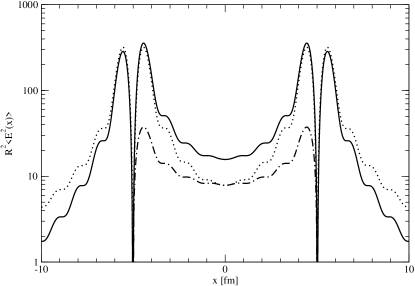
Figure 1: $R^{2}\langle{\bf E}^{2}(x)\rangle$ in units of $2b_{C}/\pi^{3}(\hbar c)^{2}$ as a function of the distance $x$ along the $Q{\bar{Q}}$ axis. We employ the $f(p)=1$ approximation. The quark and the antiquark are located at $R/2=5\mbox{ fm}$ and $-R/2=-5\mbox{ fm}$ respectively. The renormalization scale $\mu=1.1\mbox{ GeV}$ is calculated from Eq. (27) using $d(\mu)=3.5$ from Ref. as1 . The dashed line is the contribution from the two self energies, the dash-dotted line represents mutual interactions and the solid line is the total.

In Fig. 1 we show the Coulomb energy density as a function of position on the $Q{\bar{Q}}$ axis, ${\bf x}=x\hat{{\bf R}}$, for $R=|{\bf R}|=10\mbox{ fm}$. The small oscillations come from the sharp-cutoff introduced by the $\theta$-functions in Eq. (22) which produces the Bessel’s functions in Eq. (28). For a smooth cutoff, e.g. with $\theta(\mu-p)\to\exp(-p/\mu)$ in Eq. (28) one should replace $1-j_{0}(\mu|{\bf R}/2-{\bf x}|)$ by $1-\arctan(\mu|{\bf R}/2-{\bf x}|)/\mu|{\bf R}/2-{\bf x}|$. The cut-off is also responsible for the rapid variations near the quark positions, ${\bf x}=\pm R/2$.

We note that for large separations between the quarks, $R>>1/\mu$ and $x<<R$, the Coulomb energy density behaves as expected from dimensional analysis,

$$\langle{\bf E}^{2}({\bf x},R\mu\to\infty)\rangle\to{{32b_{C}}\over{\pi^{3}R^{2}}}.$$ (29)

which is consistent with linear confinement, i.e. if $\langle{\bf E}^{2}({\bf x},R\mu\to\infty)\rangle$ is integrated over ${\bf x}$ in the region $|{\bf x}|<R$ on obtains $V_{C}(R)\propto R$.

At large distances $x>>R>>1/\mu$ we obtain

$$\langle{\bf E}^{2}(|{\bf x}|/R\to\infty,R\mu\to\infty)\rangle\to{{2b_{C}R^{2}}\over{\pi^{3}{\bf x}^{4}}}.$$ (30)

If there were a finite correlation length one would expect $\langle{\bf E}^{2}(|{\bf x}|/R\to\infty,R\mu\to\infty)\rangle$ to fall-off exponentially with $|{\bf x}|$ DDS and not as a power-law. The power-law behavior obtained in Eq. (30) is again related to the difference between the $|Q{\bar{Q}},R\rangle$ state used here, which is built by adding quark sources to the vacuum and the true ground state of the $Q{\bar{Q}}$ system as discussed in Sec. IIA. In other words the profile of the chromo-electric field distribution for such a state is not expected to agree with the profile of the flux-tube or action density. To illustrate this difference, in Fig. 2 we plot the energy density as a function of the magnitude of the distance transverse to the $Q\bar{Q}$ axis, $x_{\perp}=|{\bf x}_{\perp}|$, ${\bf R}\cdot{\bf x}={\bf R}\cdot{\bf x}_{\perp}=0$.

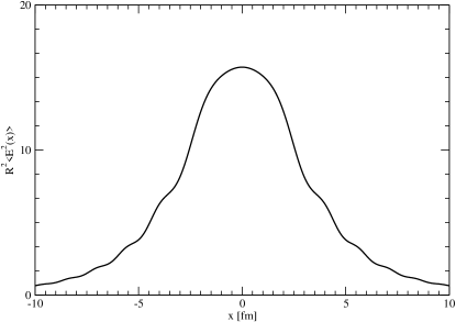
Figure 2: $R^{2}\langle{\bf E}^{2}(x)\rangle$ in units of $2b_{C}/\pi^{3}(\hbar c)^{2}$ as a function of the distance $x$ transverse to the $Q{\bar{Q}}$ axis. The units and the setting are as in Fig. 1.

Finally, in Fig. 3, we show the contour plot of the energy density as a function of the position in the $xz$ plane with quark and antiquark on the $z$ axis at $R/2$ and $-R/2$ respectively.

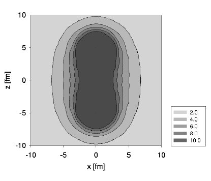
Figure 3: $R^{2}\langle{\bf E}^{2}(x)\rangle$ as a function of position in the $xz$ plane. The units and the same setting as in Fig. 1.

It is clear from Figs. 2 and 3 that a flux tube like structure emerges and from Eq. (29) that it has the correct scaling as a function of the $Q{\bar{Q}}$ separation but, as discussed above it does not have a finite correlation length (large $x$ behavior).

The field distribution for the $QQQ$ system in the $f_{L}(p)=1$ approximation is equal to the sum of three terms each representing a contribution from a $QQ$ pair. We place each of the three quarks in a corner of an equilateral triangle, ${\bf z}_{i}$, $i=1,\cdots 3$

$$\langle{\bf E}^{2}({\bf x},{\bf R}_{i})\rangle=\frac{C_{F}}{32\pi^{2}}\bigl{[}({\bf D}_{1}-{\bf D}_{2})^{2}\\ +({\bf D}_{1}-{\bf D}_{3})^{2}+({\bf D}_{2}-{\bf D}_{3})^{2}\bigr{]},$$ (31)

where

$${\bf D}_{i}={{{\bf z}_{j}-{\bf x}+{\bf r}/2}\over{|{\bf z}_{j}-{\bf x}+{\bf r}/2|}}d^{\prime}_{L}({\bf z}_{i}-{\bf x}-{\bf r}/2).$$ (32)

The contour plot of of energy density in this case is shown in Fig. 4. Even though the field originates from the two-particle correlations the net field seems to form into a “Y”-shape structure. This structure has also recently been seen to emerge in Euclidean lattice simulations.

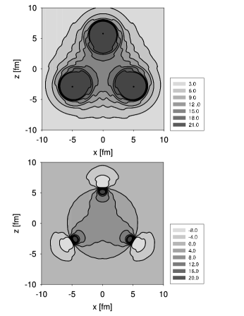
Figure 4: $R^{2}\langle{\bf E}^{2}(x)\rangle$ as a function of position in the $xz$ plane. The units and the same setting as in Fig. 1. The upper panel show the total field distribution and the lower the distribution from mutual interaction (no self-energies) only.

Finally, to study the effects of $f_{L}(p)$, in Fig. 5 we show the predictions for the $Q{\bar{Q}}$ field distribution given by Eq. (15) where we use $d(p)$ and $f(p)$ in the form given by Eq. (12) with $\alpha=1/2$ and $\beta=1$ and normalized such that $V(R)\to bR$ at large distances. Furthermore, to remove the oscillations introduced by the momentum space cutoff, we now cut the small $x$ region in coordinate space, by i) extending the upper limits of integration in Eqs. (24) and (25) to infinity and ii) cutting off the position space functions at short distances,

$$d^{\prime}_{L}(r)={2\over{\pi\alpha}}\sin(\pi\alpha/2)\Gamma(2-\alpha)\theta(r\mu-1){{\mu^{2}}\over{(\mu r)^{2-\alpha}}}$$ (33)

$$f_{L}(r)={1\over{2\pi^{2}}}\sin(\pi\beta/2)\Gamma(2-\beta)\theta(r\mu-1){{\mu^{3}}\over{(\mu r)^{3-\beta}}}.$$ (34)

Comparing Fig. 3 and Fig. 5 we observe a narrowing of the flux tube. This is to be expected as the action of $f(p)$ is to introduce additional gluonic correlations. That said, there is no major qualitative change in the field distribution.

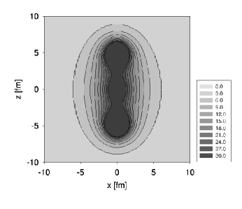
Figure 5: $R^{2}\langle{\bf E}^{2}(x)\rangle$ for $Q{\bar{Q}}$ from Eq. (23) with $\alpha=1/2$ and $\beta=1$. The units and the same setting as in Fig. 1, except that the contribution from $f(p)$ has been included.

IV Summary

We have calculated the distribution of the longitudinal chromo-electric field in the presence of static $Q{\bar{Q}}$ and $QQQ$ sources using a variational model for the ground state wave functional. Despite this wave functional having no string-like correlations a flux tube like picture does emerge. In particular the on-axis energy density of the $Q{\bar{Q}}$ system behaves as $b_{c}/R^{2}$ for large inter-quark separation, $R$ and the field falls off like $b_{c}R^{2}/x^{4}$ at large distances from the center of mass of the $Q{\bar{Q}}$ system, $x$. This is weaker than in the Abelian case ($\sim R^{2}/x^{6}$) and implies that moments of the average transverse spread of the tube, defined as proportional to $\langle|x_{\perp}|^{n}{\bf E}^{2}(z,x_{\perp})\rangle$, are finite for $n<2$ only. Thus there is no finite correlation length for the longitudinal component of the chromo-electric field, as expected for the state which does not take into account screening of the Coulomb line by the transverse gluons (flux tube). This also leads to large Van der Waals forces, which is bothersome, but it is consistent with the scenario of “no confinement without Coulomb confinement” of Zwanziger. The Coulomb potential leads to a variational (stronger) upper bound to the true confining interaction.

Similar behavior at large distances is also true for the three quark sources, except that here we find the emergence of the “Y”-shape junction. This is consistent with lattice simulations, but is remarkable in our case as it arises from two-body forces. It will be interesting to examine field distributions which include transverse field excitations. In that case the only lattice results available are for the potential, not for the field distributions. Finally we note that, since the mean field calculation provides a variational upper bound, the long range behavior of the field distribution falls-off more slowly than expected for the Van der Waals force. Certainly as the complete string develops this is expected to disappear and it would be interesting to build a string-like model for the ansatz ground state to verify this assertion.

- (1) N. H. Christ and T. D. Lee, Phys. Rev. D 22, 939 (1980) [Phys. Scripta 23, 970 (1981)].
- (2) D. Zwanziger, Nucl. Phys. B 485, 185 (1997) [arXiv:hep-th/9603203].
- (3) A. Cucchieri and D. Zwanziger, Phys. Rev. Lett. 78, 3814 (1997) [arXiv:hep-th/9607224].
- (4) A. P. Szczepaniak and E. S. Swanson, Phys. Rev. D 65, 025012 (2002) [arXiv:hep-ph/0107078].
- (5) A. P. Szczepaniak and E. S. Swanson, Phys. Rev. D 62, 094027 (2000) [arXiv:hep-ph/0005083].
- (6) A. P. Szczepaniak and E. S. Swanson, Phys. Rev. D 55, 1578 (1997) [arXiv:hep-ph/9609525].
- (7) J. Greensite, S. Olejnik and D. Zwanziger, arXiv:hep-lat/0401003.
- (8) L. Del Debbio, A. Di Giacomo and Y. A. Simonov, Phys. Lett. B 332, 111 (1994) [arXiv:hep-lat/9403016].
- (9) A. P. Szczepaniak, arXiv:hep-ph/0306030.
- (10) C. Feuchter and H. Reinhardt, arXiv:hep-th/0402106.
- (11) A. R. Swift, Phys. Rev. D 38, 668 (1988).
- (12) T. T. Takahashi, H. Matsufuru, Y. Nemoto and H. Suganuma, Phys. Rev. Lett. 86, 18 (2001) [arXiv:hep-lat/0006005]; Phys. Rev. D 65, 114509 (2002) [arXiv:hep-lat/0204011]; T. T. Takahashi and H. Suganuma, Phys. Rev. Lett. 90, 182001 (2003).
- (13) V.G. Bornyakov et al. [DIK Collaboration], arXiv:hep-lat/0401026.
- (14) C. Alexandrou, P. De Forcrand and A. Tsapalis, Phys. Rev. D 65, 054503 (2002) [arXiv:hep-lat/0107006].
- (15) A. I. Shoshi, F. D. Steffen, H. G. Dosch and H. J. Pirner, Phys. Rev. D 68, 074004 (2003) [arXiv:hep-ph/0211287].
- (16) D. S. Kuzmenko and Y. A. Simonov, Phys. Atom. Nucl. 66, 950 (2003) [Yad. Fiz. 66, 983 (2003)] [arXiv:hep-ph/0202277].
- (17) J. M. Cornwall, Phys. Rev. D 69, 065013 (2004) [arXiv:hep-th/0305101].
- (18) D. Zwanziger, Phys. Rev. Lett. 90, 102001 (2003) [arXiv:hep-lat/0209105].
- (19) D. Zwanziger, arXiv:hep-ph/0312254.
- (20) J. Greensite and S. Olejnik, Phys. Rev. D 67, 094503 (2003) [arXiv:hep-lat/0302018].