Time-to-space conversion in quantum field theory of flavor mixing

Abstract

We consider the problem of time-to-space conversion in quantum field theory of flavor mixing using a generalization of the wave-packet method in quantum mechanics. We work entirely within the canonical formalism of creation and annihilation operators that allows us, unlike the usual wave-packet formulation, to include the nontrivial effect due to flavor condensation in the vacuum.

I Introduction

The mixing of quantum fields plays an important role in the phenomenology of high-energy physics [1, 2, 3]. Mixing of both $K^{0}\bar{K}^{0}$ and $B^{0}\bar{B}^{0}$ bosons provides the evidence of $CP$ violation in weak interaction [4] and $\eta\eta\prime$ boson mixing in the $SU(3)$ flavor group gives a unique opportunity to investigate the nontrivial QCD vacuum and fill the gap between QCD and the constituent quark model. In the fermion sector, neutrino mixing and oscillations provide striking evidences of neutrino masses and are the most likely solution of the famous solar neutrino puzzle [5, 6, 7]. In addition, the standard model incorporates the mixing of fermion fields through the Kobayashi-Maskawa (CKM) mixing of three quark flavors, a generalization of the original Cabibbo mixing matrix between $d$ and $s$ quarks [8, 9, 10, 11].

From the theoretical point of view the field theory of mixing is important since this is one of a few examples where the quantum field theory can be solved exactly. Moreover, the field-theoretical treatment of mixing touches the fundamental questions of the quantization of interacting fields, which are not yet fully understood. It also allows to improve the accuracy of ordinary perturbation theory, e.g. the mixed-Hamiltonian dynamics can be used for partial re-summation of ordinary perturbation series in weak interactions.

Recently, the importance of mixing transformations has prompted a fundamental examination from a field-theoretical perspective. It was found that the flavor mixing in quantum field theory introduces very non-trivial relationships between the interacting and non-interacting (free) fields, which lead to unitary inequivalence between the Fock space of the interacting fields and that of the free fields [14, 18, 22, 23]. This is different from the conventional perturbation theory where one would expect the vacuum of the interacting fields to be essentially similar to one of the free fields (up to a phase factor $e^{iS_{0}}$ [24, 25]). The investigation of two-field unitary mixing in the fermion sector by Blasone and Vitiello [18, 19, 20, 21] demonstrated a rich structure of the interacting-field vacuum as SU(2) coherent state and altered the oscillation formula to include the antiparticle degrees of freedom. Subsequent analysis of the boson case revealed a similar but much richer structure of the vacuum of the interacting fields [14, 15, 16]. Especially, the pole structure in the inner product between the vacuum of the free theory and the vacuum of the interacting theory was found and related to the convergence radius of the perturbation series [15]. Attempts to look at the mixing of more than two flavors have also been carried out and a general framework for such a theory has been suggested by Ji and Mishchenko [13]. Also, mathematically rigorous study of this case has been offered by Hannabuss and Latimer [12].

Surprisingly, although a wide research effort has been undertaken in this direction, an important aspect of the formulation is still left uncultivated. Namely, the oscillation formulas in most cases are obtained theoretically in terms of time oscillations, while the experimental measurements are only carried out in terms of space oscillations. Despite seeming triviality of the question, it is indeed not an easy one and certain controversy always existed in the literature about the appropriate way of handling this task. Naively speaking, a quantity of dimension of speed must be involved in the conversion, however there are at least two such quantities in the flavor mixing problem [26]. It was argued that the correct way to do such conversion was to equal the energies of the mixed particles thus allowing the uncertainty in 3-momenta to form a wave-packet. At the higher level of rigor, no doubt, the most consistent argument in quantum mechanics comes from the method of wave-packets, where the flavor particles are treated as waves with not just uncertainty in the 3-momentum, but also in the energy [27, 28]. Within this approach the correct oscillation length is recovered and also the concept of correlation length is introduced. As one becomes aware of nontrivial role of antiparticles in field-theoretical flavor mixing [13, 18], a natural question arises if and how such effects would manifest themselves in space-dimensions. Therefore, in this work we would like to build a field-theoretical development analogous to quantum mechanical wave-packet method and apply it to study time-to-space conversion for the field-theoretical result in flavor mixing.

We must note that recently the wave-packet approach has been extended to field theory by means of using the field-theoretical flavor propagation functions [29]. We should stress, however, that such treatment is essentially different from ours in that the flavor propagators were defined via the expectation value on the vacuum of the free-fields and as such have the problem of total probability non-conservation pointed out by Blasone and Vitiello [17, 19]. It thus lacks the capacity to include nonperturbative effects due to nontrivial flavor condensation in vacuum found in [13, 14, 15, 16, 17, 18, 19].

In this paper, we analyze the problem of time-to-space conversion from the same ”wave-packets” point of view, but entirely within the canonical framework of creation/annihilation operators. This allows us to build the theory as an extension of the general formalism [13] and, thus, to consider the nontrivial vacuum effects. In particular, the high-frequency contribution on top of usual Ponte-Corvo oscillations is retained and its effect in space-dimensions is studied.

In the next section (Section II) we present the canonical framework for the flavor oscillations in space-time and generalize the quantum mechanical wave-packet method to the quantum field theory. In Section III, as a demonstration of this formalism, we discuss the space-oscillations in the system of two (pseudo)scalar mesons such as $\eta$ and $\eta^{\prime}$ and present the relevant numerical results. Conclusion follows in Section IV.

II Oscillations of flavor in space-time

We begin our study with a simple example. Let us consider a particle created initially in quantum state $\left|i\right\rangle$ and propagated in space and time. The number of particles of sort $\rho$ to be detected at the space-time position $x=(t,{\bf x})$ is given by

$$N_{\rho}(x)=\left\langle i|a_{\rho}^{\dagger}(x)a_{\rho}(x)|i\right\rangle,$$ (1)

where $a^{\dagger}_{\rho}(x)(a_{\rho}(x))$ is creation (annihilation) operator for particles of sort $\rho$ at space-time position $x$. This can be defined via creation (annihilation) operators for given momentum ${\bf k}$

$$a_{\rho}^{\dagger}(t,{\bf x})=\sum\limits_{{\bf k}}\frac{1}{\sqrt{2\omega_{\rho{\bf k}}}}e^{-i{\bf kx}}a_{\rho,{\bf k}}^{\dagger}(t).$$ (2)

Substituting the definition given by Eq.(2) into Eq.(1), one obtains

$$N_{\rho}(x)=\sum\limits_{{\bf k,k}^{\prime}}\frac{e^{i({\bf k}^{\prime}-{\bf k}){\bf x}}}{2\sqrt{\omega_{\rho{\bf k}}\omega_{\rho{\bf k}^{\prime}}}}\left\langle i|a_{\rho,{\bf k}}^{\dagger}(t)a_{\rho,{\bf k}^{\prime}}(t)|i\right\rangle.$$ (3)

We thus find that the number of particles expected at the space-time position $x$ can be found using Eq.(3) once $\left\langle i|a_{\rho,{\bf k}}^{\dagger}(t)a_{\rho,{\bf k}^{\prime}}(t)|i\right\rangle$ is known for all ${\bf k}$ and ${\bf k}^{\prime}$.

In the above example, it is instructive to recognize a more general problem. First of all, note that Eq.(3) is analogous to conventional probability density $|\Psi(x)|^{2}$; in the case of free fields it, indeed, yields the square of the Feynman propagation amplitude

$$|\Delta_{F}(z)|^{2}=\left|\sum\limits_{{\bf k}}\frac{e^{i({\bf kz}-\omega_{{\bf k}}z^{0})}}{2\omega_{{\bf k}}}\right|^{2}=|\int\frac{d^{d}k}{(2\pi)^{d}}\frac{ie^{-ikz}}{k^{2}-m^{2}+i\epsilon}|^{2}.$$ (4)

Unlike the Feynman propagation amplitude, however, Eq.(3) generalizes naturally to the case when the total number of particles of a given sort is not conserved, as is, essentially, in any flavor oscillation theory.

Now, following closely the structure of the states in field theory of flavor mixing [13, 16, 18], let us introduce the initial state $\left|i\right\rangle$ for a system with $N$ sorts (flavors) of particles by

$$\left|i\right\rangle=\sum\limits_{\rho=1;{\bf k}}^{N}(g_{\rho,{\bf k}}a_{\rho,{\bf k}}^{\dagger}+h_{\rho,{\bf k}}b_{\rho,-{\bf k}}^{\dagger})\left|\Omega\right\rangle,$$ (5)

where $a_{\rho,{\bf k}}^{\dagger}$, $b_{\rho,-{\bf k}}^{\dagger}$ are the particle and antiparticle creation operators for sort (flavor) $\rho$ and $\left|\Omega\right\rangle$ is the flavor vacuum state annihilated by all $a_{\rho,{\bf k}}$, $b_{\rho,{\bf k}}$. Eq.(5), essentially, represents a single particle initially created in a state such that the probability to observe it as sort $\rho$-particle (antiparticle) is simply $|g_{\rho,{\bf k}}|^{2}$ ($|h_{\rho,-{\bf k}}|^{2}$). Then, $2N$ functions $g_{\rho,{\bf k}},h_{\rho,{\bf k}}$ are the form-factors for the initial state $\left|i\right\rangle$ . For notation convenience we shall adopt following convention. We will let $\alpha$ be both positive and negative ($\alpha=-N,\ldots,N$, excluding $\alpha=0$) with negative $\alpha$ enumerating antiparticles and positive $\alpha$ enumerating particles, respectively. In this notation

$$\left|i\right\rangle=\sum\limits_{\alpha=-N;{\bf k}}^{N}f_{\alpha,{\bf k}}a_{\alpha,{\bf k}}^{\dagger}\left|\Omega\right\rangle,$$ (6)

where for convenience we have introduced $a_{\alpha,{\bf k}}^{{\dagger}}:=a^{\dagger}_{\alpha,{\bf k}}$ for $\alpha>0$ and $a_{\alpha,{\bf k}}^{\dagger}:=b^{\dagger}_{-\alpha,-{\bf k}}$ for $\alpha<0$. Analogously, $f_{\alpha,{\bf k}}:=g_{\alpha,{\bf k}}$ for $\alpha>0$ and $f_{\alpha,{\bf k}}:=h_{-\alpha,{\bf k}}$ for $\alpha<0$. Also, from now on, in summations over $\alpha$ we imply $\alpha\neq 0$.

From Eq.(6), we may further introduce the creation operator for form-factor ${F}=\{f_{\alpha,{\bf k}},\alpha=-N\dots-1,1\dots N\}$ as

$$a^{\dagger}({F})=\sum\limits_{\alpha=-N;{\bf k}}^{N}f_{\alpha,{\bf k}}a_{\alpha,{\bf k}}^{\dagger},$$ (7)

so that concisely $\left|i\right\rangle=a^{\dagger}({F})\left|\Omega\right\rangle$. It is straightforward to obtain the non-equal time commutation/anticommutation relationships for $a({F})$ and $a^{\dagger}(G)$

$$\begin{array}[]{c}[a({F}),a^{\dagger}({G})]_{\pm,\text{equal time}}=\sum\limits_{\alpha=-N;{\bf k}}^{N}f_{\alpha,{\bf k}}^{*}g_{\alpha,{\bf k}}=(f,g)_{I},\\ [a_{t}({F}),a^{\dagger}({G})]_{\pm}=\sum\limits_{\alpha,\beta=-N;{\bf k}}^{N}f_{\alpha,{\bf k}}^{*}{\cal F}_{\alpha\beta;{\bf k}}(t)g_{\beta,{\bf k}}=(f,g)_{\cal F},\\ [a_{t}({F}),a({G})]_{\pm}=\sum\limits_{\alpha,\beta=-N;{\bf k}}^{N}f_{\alpha,{\bf k}}^{*}{\cal G}_{\alpha\beta;{\bf k}}(t)g^{*}_{\beta,{\bf k}}=(f,g^{*})_{\cal G},\end{array}$$ (8)

where $\pm$ in $[$ $]_{\pm}$ corresponds to commutation/anticommutation and the inner product is defined by $(f,g)_{\cal A}=\sum\limits_{\alpha,\beta=-N;{\bf k}}^{N}f_{\alpha,{\bf k}}^{*}{\cal A}_{\alpha\beta;{\bf k}}(t)g_{\beta,{\bf k}}$. ${\cal F}_{\alpha\beta;{\bf k}}(t)$, ${\cal G}_{\alpha\beta;{\bf k}}(t)$ are the non-equal time commutators/anticommutators for momentum ${\bf k}$ as introduced in [13],

$$\begin{array}[]{c}[a_{\alpha,{\bf k}}(t),a^{\dagger}_{\beta,{\bf k^{\prime}}}]_{\pm}={\cal F}_{\alpha\beta;{\bf k}}(t)\delta({\bf k-k^{\prime}})\cr[a_{\alpha,{\bf k}}(t),a_{\beta,{\bf k^{\prime}}}]_{\pm}={\cal G}_{\alpha\beta;{\bf k}}(t)\delta({\bf k-k^{\prime}}).\end{array}$$ (9)

In the notations used in our general field theory of flavor mixing [13], for given momentum k,

$$\begin{array}[]{c}{\cal G}_{\alpha\beta}(t)=\left\{\begin{array}[]{c}G_{-\alpha,\beta}(t),\alpha<0,\beta>0;\\ \eta G_{-\beta,\alpha}(-t),\alpha>0,\beta<0;\\ 0,\text{ otherwise.}\end{array}\right.=\left(\begin{array}[]{cc}0&\eta G^{T}(-t)\\ G(t)&0\end{array}\right),\\ {\cal F}_{\alpha\beta}(t)=\left\{\begin{array}[]{c}F_{\alpha,\beta}(t),\alpha>0,\beta>0;\\ F_{-\beta,-\alpha}(t),\alpha<0,\beta<0;\\ 0,\text{ otherwise.}\end{array}\right|=\left(\begin{array}[]{cc}F(t)&0\\ 0&F^{T}(t)\end{array}\right),\end{array}$$ (10)

where $\eta=(-1)^{2S}$ with $S$ being the spin of the mixed fields ($\eta$ is +1 for bosons and -1 for fermions), and $F_{\alpha\beta}$ and $G_{\alpha\beta}$ in terms of original flavor creation/annihilation operators are defined by

$$\begin{array}[]{rl}F_{\alpha\beta;{\bf k}}(t)&=[a_{\alpha,{\bf k}}(t),a_{\beta,{\bf k}}^{\dagger}]_{\pm}\\ &=[b_{\beta{\bf,-k}}(t),b_{\alpha{\bf,-k}}^{\dagger}]_{\pm},\\ G_{\alpha\beta;{\bf k}}(t)&=[b_{\alpha,-{\bf k}}(t),a_{\beta,{\bf k}}]_{\pm}.\end{array}$$ (11)

The primary interest of this paper is the process in which a ”flavor” particle is created in some initial state $|i\rangle$ with form-factor given by $G=\{g_{\alpha,{\bf k}}\}$ and is detected at time $t$ as state $|f\rangle$ with form-factor $F=\{f_{\alpha,{\bf k}}\}$. In that case the object of interest is the number operator $N_{F}(t)=a_{t}^{\dagger}(F)a_{t}(F)$

$$\left\langle i|N_{F}(t)|i\right\rangle=\left\langle\Omega|a(G)a_{t}^{\dagger}(F)a_{t}(F)a^{\dagger}(G)|\Omega\right\rangle.$$ (12)

Using the machinery we just have introduced and after simple algebra, we find

$$\begin{array}[]{rl}\left\langle i|N_{F}(t)|i\right\rangle&=|[a_{t}(F),a^{\dagger}(G)]_{\pm}|^{2}+\eta|[a(G),a_{t}(F)]_{\pm}|^{2}+\left\langle a_{t}^{\dagger}(F)a_{t}(F)\right\rangle,\\ &=|(f,g)_{\cal F}|^{2}+\eta|(f,g^{*})_{\cal G}|^{2}+(f,f)_{\cal Z},\end{array}$$ (13)

where the last term is related to flavor condensation in vacuum

$$\begin{array}[]{c}(f,f)_{\cal Z}=\left\langle a_{t}^{\dagger}(F)a_{t}(F)\right\rangle=\sum\limits_{\alpha=-N;{\bf k}}^{N}f_{\alpha,{\bf k}}{\cal Z}_{\alpha,{\bf k}}(t)f_{\alpha,{\bf k}},\cr{\cal Z}_{\alpha,{\bf k}}(t)=\left\langle\Omega|a_{\alpha,{\bf k}}^{\dagger}(t)a_{\alpha,{\bf k}}(t)|\Omega\right\rangle.\end{array}$$ (14)

Generally, this term is not zero for $t\neq 0$ as was found in the works mentioned above. Indeed, for many choices of $F$ it is infinite. On the other hand, one may notice that this contribution is independent from the initial state $|i\rangle$ and thus may be interpreted as the background due to the vacuum condensation picked up by the detector itself. In this case one shall renormalize it by defining

$$\left\langle i|N_{F}(t)|i\right\rangle_{r}=\left\langle i|N_{F}(t)|i\right\rangle-\left\langle\Omega|N_{F}(t)|\Omega\right\rangle.$$

In what follows, we will understand $\left\langle i|N_{F}(t)|i\right\rangle$ by such a renormalized expectation value. In an extended notation, explained above, it is given by

$$\begin{array}[]{c}\left\langle i|N_{F}(t)|i\right\rangle_{r}=|\sum\limits_{\alpha,\beta=-N;{\bf k}}^{N}f_{\alpha,{\bf k}}^{*}{\cal F}_{\alpha\beta;{\bf k}}(t)g_{\beta,{\bf k}}|^{2}+\eta|\sum\limits_{\alpha,\beta=-N;{\bf k}}^{N}f_{\alpha,{\bf k}}^{*}{\cal G}_{\alpha\beta;{\bf k}}(t)g^{*}_{\beta,{\bf k}}|^{2}.\end{array}$$ (15)

In the previous works special attention was paid to the oscillations of flavor charge which can be immediately related to the observables in the theory. Oscillations of flavor charge can be obtained from Eq.(13). For the case of detection of a single particle with flavor $\beta$ and form-factor $f(\bf k)$

$$Q_{\beta}(t)=N_{[\beta]}(t)-N_{{[-\beta]}}(t),$$ (16)

where $[\beta]=\{f_{\alpha,{\bf k}}=f({\bf k})\delta_{\alpha,\beta}\}$ and ${[-\beta]}=\{f_{\alpha,{\bf k}}=f({-\bf k})\delta_{-\alpha,\beta}\}$.

It is straightforward to derive from Eqs.(15) and (16) the oscillations in space, in which case the detector shall be characterized by the form-factor; $[\beta]=\{f_{\alpha,{\bf k}}=\frac{e^{-i{\bf kx}}}{\sqrt{2\omega_{\beta{\bf k}}}}\delta_{\alpha,\beta}\}$ for a single particle of sort $\beta$ or $[-\beta]=\{f_{\alpha,{\bf k}}=\frac{e^{i{\bf kx}}}{\sqrt{2\omega_{\beta{\bf k}}}}\delta_{-\alpha,\beta}\}$ for a single anti-particle of the same sort:

$$\begin{array}[]{rl}\left\langle i|N_{\beta}(t,{\bf x})|i\right\rangle_{r}=&|\sum\limits_{\alpha;{\bf k}}\frac{e^{i{\bf kx}}}{({2\omega_{\beta{\bf k}}})^{1/2}}{{\cal F}_{\beta\alpha;{\bf k}}(t)g_{\alpha,{\bf k}}}|^{2}+\eta|\sum\limits_{\alpha;{\bf k}}\frac{e^{i{\bf kx}}}{({2\omega_{\beta{\bf k}}})^{1/2}}{{\cal G}_{\beta\alpha;{\bf k}}(t)g^{*}_{\alpha,{\bf k}}}|^{2},\\ \left\langle i|N_{-\beta}(t,{\bf x})|i\right\rangle_{r}=&|\sum\limits_{\alpha;{\bf k}}\frac{e^{-i{\bf kx}}}{({2\omega_{\beta{\bf k}}})^{1/2}}{{\cal F}_{-\beta\alpha;{\bf k}}(t)g_{\alpha,{\bf k}}}|^{2}+\eta|\sum\limits_{\alpha;{\bf k}}\frac{e^{-i{\bf kx}}}{({2\omega_{\beta{\bf k}}})^{1/2}}{{\cal G}_{-\beta\alpha;{\bf k}}(t)g^{*}_{\alpha,{\bf k}}}|^{2},\\ \left\langle i|Q_{\beta}(t,{\bf x})|i\right\rangle=&\left\langle i|N_{\beta}(t,{\bf x})|i\right\rangle-\left\langle i|N_{-{\beta}}(t,{\bf x})|i\right\rangle.\end{array}$$ (17)

As in the quantum-mechanical wave-packet method, our final result depends on the kind of initial state assumed for the flavor particle. For example, one may consider the initial state as a state with definite momentum ${\bf k}$ and definite flavor $\beta$,

$$\left\langle\beta{\bf k}|N_{\alpha}(t,{\bf x})|\beta{\bf k}\right\rangle_{r}=(2\omega_{\alpha{\bf k}}\omega_{\beta{\bf k}})^{-1}{|{\cal F}_{\alpha\beta;{\bf k}}(t)|^{2}}+\eta(2\omega_{\alpha{\bf k}}\omega_{\beta{\bf k}})^{-1}{|{\cal G}_{\alpha\beta;{\bf k}}(t)|^{2}}.$$ (18)

This, however, has no dependence on ${\bf x}$ and thus one can not observe any space oscillation. One also might consider a particle of sort $\beta$ created at position ${\bf x}^{\prime}$ and observed at position ${\bf x}$ at time $t$ as a particle of sort $\alpha$. For that case one finds

$$\begin{array}[]{c}\left\langle\beta{\bf x}^{\prime}|N_{\alpha}(t,{\bf x})|\beta{\bf x}^{\prime}\right\rangle_{r}=|\sum\limits_{{\bf k}}\frac{e^{i({\bf x}-{\bf x}^{\prime}){\bf k}}}{2\sqrt{\omega_{\alpha{\bf k}}\omega_{\beta{\bf k}}}}{{\cal F}_{\alpha\beta;{\bf k}}(t)}|^{2}+\eta|\sum\limits_{{\bf k}}\frac{e^{i({\bf x}-{\bf x}^{\prime}){\bf k}}}{2\sqrt{\omega_{\alpha{\bf k}}\omega_{\beta{\bf k}}}}{{\cal G}_{\alpha\beta;{\bf k}}(t)}|^{2}\\ =|^{*}{\cal F}_{\alpha\beta}({\bf x}^{\prime}-{\bf x},t)|^{2}+\eta|^{*}{\cal G}_{\alpha\beta}({\bf x}^{\prime}-{\bf x},t)|^{2},\end{array}$$ (19)

where ${}^{*}{\cal F}({\bf z})$ is the Fourier transform of $(2\sqrt{\omega_{\alpha{\bf k}}\omega_{\beta{\bf k}}})^{-1}{{\cal F}({\bf k})}$ and ${}^{*}{\cal G}$ is defined similarly.

In practice, however, we are interested in the case when a flavor particle was produced originally in a small (but finite) region of space with (nonzero) momentum ${\bf k}$. This can be represented by a well-peaked initial state $|i\rangle$ with form-factor $g({\bf k})$ such that a single particle of sort $\beta$ appears as a wave-packet of momentum ${\bf k}_{0}$ with small dispersion $\sigma$. Taking now the explicit form of ${\cal F}$ and ${\cal G}$ from [13] and leaving the detector point-like, we obtain

$$\begin{array}[]{c}\left\langle\beta g|N_{\alpha}(t,{\bf x})|\beta g\right\rangle_{r}=\left|\sum\limits_{\gamma}(a_{\alpha\beta;\gamma}e^{-iw_{\gamma}t}e^{-\sigma^{2}({\bf v}_{\gamma}t-{\bf x})^{2}/2}+b_{\alpha\beta;\gamma}e^{iw_{\gamma}t}e^{-\sigma^{2}(-{\bf v}_{\gamma}t-{\bf x})^{2}/2})\right|^{2}+\\ \eta\left|\sum\limits_{\gamma}(c_{\alpha\beta;\gamma}e^{-iw_{\gamma}t}e^{-\sigma^{2}({\bf v}_{\gamma}t-{\bf x})^{2}/2}+d_{\alpha\beta;\gamma}e^{iw_{\gamma}t}e^{-\sigma^{2}(-{\bf v}_{\gamma}t-{\bf x})^{2}/2})\right|^{2};\\ {\bf v}_{\gamma}=\frac{dw_{\gamma}({\bf k})}{d{\bf k}}|_{{\bf k}_{0}}.\end{array}$$ (20)

In the above derivation we used following identity which can be proved using stationary phase approximation for function $g({\bf k})$ sharply peaked around ${\bf k=k}_{0}$ and slow-varying functions $f({\bf k})$ and $S({\bf k})$,

$$\begin{array}[]{c}\int d{\bf k}g({\bf k})f({\bf k})e^{iS({\bf k})}e^{i{\bf kx}}\approx(2\pi\sigma^{2})^{3/2}g({\bf k}_{0})f({\bf k}_{0})e^{i(S({\bf k}_{0})+{\bf k}_{0}{\bf x})}\exp(-\sigma^{2}({\bf x}+{\bf\vec{\nabla}}S({\bf k}_{0}))^{2}/2),\\ \sigma^{2}=-\frac{g({\bf k}_{0})}{g^{\prime\prime}({\bf k}_{0})}.\end{array}$$ (21)

The explicit form of ${\cal F}$ and ${\cal G}$ is taken as (see [13] for specific values of $a_{\alpha,\beta;\gamma}({\bf k}),b_{\alpha,\beta;\gamma}({\bf k}),c_{\alpha,\beta;\gamma}({\bf k}),d_{\alpha,\beta;\gamma}({\bf k})$)

$$\begin{array}[]{c}({\sqrt{2\omega_{\alpha{\bf k}}}})^{-1}{{\cal F}_{\alpha\beta,{\bf k}}(t)}=\sum\limits_{\gamma=1}^{N}(a_{\alpha\beta;\gamma}({\bf k})e^{-iw_{\gamma{\bf k}}t}+b_{\alpha\beta;\gamma}({\bf k})e^{iw_{\gamma{\bf k}}t}),\\ ({\sqrt{2\omega_{\alpha{\bf k}}}})^{-1}{{\cal G}_{\alpha\beta,{\bf k}}(t)}=\sum\limits_{\gamma=1}^{N}(c_{\alpha\beta;\gamma}({\bf k})e^{-iw_{\gamma{\bf k}}t}+d_{\alpha\beta;\gamma}({\bf k})e^{iw_{\gamma{\bf k}}t}),\end{array}$$ (22)

and all amplitudes in Eq.(20) are taken at ${\bf k=k}_{0}$. Eq.(20) physically represents the expectation value for the number of $\alpha$-sort particles observed at position ${\bf x}$ at time $t$ when a single particle of sort $\beta$ and form-factor $g({\bf k})$ had been emitted. What we observe, hence, is a single wave-packet propagating through the space: i.e. one can see that $\left\langle\beta g|N_{t}(\alpha{\bf x})|\beta g\right\rangle$ reaches maximum only when the ”center” of the wave-packet passes over the observation point ${\bf x}$

$$\langle{\bf v}\rangle t\approx{\bf x}\text{ or }\langle-{\bf v}\rangle t\approx{\bf x}.$$ (23)

To explicitly observe space oscillations, one should take an average over time in Eq.(17) which would correspond to a observation continuous in time,

$$\begin{array}[]{rl}W_{g}(f)&\sim\lim\limits_{T\rightarrow\infty}\int\limits_{T}dt\left\langle g|N(t,F)|g\right\rangle_{r}\\ &\sim\lim\limits_{T\rightarrow\infty}\int\limits_{T}dt\left(|\sum\limits_{\beta;{\bf k}}\frac{e^{i{\bf kx}}}{\sqrt{2\omega_{\alpha{\bf k}}}}{\cal F}_{\alpha\beta;{\bf k}}(t)g_{\beta,{\bf k}}|^{2}+\eta|\sum\limits_{\beta;{\bf k}}\frac{e^{i{\bf kx}}}{\sqrt{2\omega_{\alpha{\bf k}}}}{\cal G}_{\alpha\beta;{\bf k}}(t)g^{*}_{\beta,{\bf k}}|^{2}\right).\end{array}$$ (24)

Using Eq.(22), we may rewrite this as

$$\begin{array}[]{c}\sum\limits_{\gamma,\gamma^{\prime}}\int\int d{\bf k}d{\bf k}^{\prime}\delta(w_{\gamma{\bf k}}-w_{\gamma^{\prime}{\bf k}^{\prime}})[(a_{\alpha\beta;\gamma}({\bf k})a_{\alpha\beta;\gamma^{\prime}}^{*}({\bf k}^{\prime})+b_{\alpha\beta;\gamma}({\bf k})b_{\alpha\beta;\gamma^{\prime}}^{*}({\bf k}^{\prime}))+\\ \eta(c_{\alpha\beta;\gamma}({\bf k})c_{\alpha\beta;\gamma^{\prime}}^{*}({\bf k}^{\prime})+d_{\alpha\beta;\gamma}({\bf k})d_{\alpha\beta;\gamma^{\prime}}^{*}({\bf k}^{\prime}))]g_{\beta,{\bf k}}g^{*}_{\beta,{\bf k}^{\prime}}e^{i({\bf k}-{\bf k}^{\prime}){\bf x}}.\end{array}$$

When the mass difference $m_{\gamma}^{2}-m_{\gamma^{\prime}}^{2}$ is small, the functional

$$\begin{array}[]{c}\delta(w_{\gamma{\bf k}}-w_{\gamma^{\prime}{\bf k}^{\prime}})[(a_{\alpha\beta;\gamma}({\bf k})a_{\alpha\beta;\gamma^{\prime}}^{*}({\bf k}^{\prime})+b_{\alpha\beta;\gamma}({\bf k})b_{\alpha\beta;\gamma^{\prime}}^{*}({\bf k}^{\prime}))\pm\\ (c_{\alpha\beta;\gamma}({\bf k})c_{\alpha\beta;\gamma^{\prime}}^{*}({\bf k}^{\prime})+d_{\alpha\beta;\gamma}({\bf k})d_{\alpha\beta;\gamma^{\prime}}^{*}({\bf k}^{\prime}))]g_{\beta,{\bf k}}g^{*}_{\beta,{\bf k}^{\prime}}e^{i({\bf k}-{\bf k}^{\prime}){\bf x}}\end{array}$$ (25)

has its maximum at ${\bf k}\approx{\bf k^{\prime}}\approx{\bf k}_{0}$. Then for the initial single flavor particle $\beta$ with sharply-peaked $g_{\beta,{\bf k}}$ we can use the stationary phase approximation again to find

$$\begin{array}[]{rll}W({\bf x})&\sim\sum\limits_{\gamma,\gamma^{\prime}}&\left[(a_{\alpha\beta;\gamma}({\bf k})a^{*}_{\alpha\beta;\gamma^{\prime}}({\bf k})+b_{\alpha\beta;\gamma}({\bf k})b^{*}_{\alpha\beta;\gamma^{\prime}}({\bf k}))\right.\cr&&+\left.\eta(c_{\alpha\beta;\gamma}({\bf k})c^{*}_{\alpha\beta;\gamma^{\prime}}({\bf k})+d_{\alpha\beta;\gamma}({\bf k})d^{*}_{\alpha\beta;\gamma^{\prime}}({\bf k}))\right]e^{-(\frac{\Delta k_{\gamma\gamma^{\prime}}}{2k_{0}})^{2}\sigma^{2}{\bf x}^{2}+i\Delta{\bf k}_{\gamma\gamma^{\prime}}{\bf x}},\end{array}$$ (26)

where ${\bf k}\approx{\bf k}_{0}$, $\Delta{\bf k}_{\gamma\gamma^{\prime}}=\frac{\Delta m^{2}_{\gamma\gamma^{\prime}}}{2|{\bf k_{0}}|}\hat{\bf k}_{0}=\frac{m^{2}_{\gamma}-m^{2}_{\gamma^{\prime}}}{2|{\bf k}_{0}|}\hat{\bf k}_{0}$.

For the mixing of two flavors we recover the oscillation length as

$$L\approx\frac{2k}{\Delta m_{12}^{2}}.$$ (27)

We should point out here that the field-theoretical corrections are found only to change the amplitude of the oscillations while no major distortion in the structure of oscillations is found. This is quite different from the case of the flavor oscillations in time where the additional high-frequency term was prominent. Indeed, we found that only one mode of space oscillations, with the wave-length related to $\Delta m_{\gamma\gamma^{\prime}}^{2}$ by Eq.(27), survives the average over time. While this result may be in part attributed to the approximation we used, one may also notice that in Eq.(24)

$$\int dte^{i(\omega_{\gamma{\bf k}}\pm\omega_{\gamma^{\prime}{\bf k^{\prime}}})t}$$

is not equal to zero only when $\omega_{\gamma{\bf k}}\pm\omega_{\gamma^{\prime}{\bf k^{\prime}}}=0$ and for that the frequencies must come in with the opposite signs. Thus, no high-frequency terms may survive the integration over time. However, field-theoretical effect is still noticeable in the shape of the oscillations as we will show below.

III Space-oscillations in mixing of two mesons

In this section we shall investigate in greater details the effect of the field-theoretical corrections on the shape of the oscillations of flavor charge in space. For that, we will apply the formalism developed above to the mixing of two spin-zero particles created initially in a state with given flavor and a gaussian form-factor.

In the case of two spin-zero fields the mixing can be described completely with a single mixing angle which relates the flavor fields ($\varphi$) to the free fields ($\phi$) by

$$\left(\begin{array}[]{c}\varphi_{1}\\ \varphi_{2}\end{array}\right)=\left(\begin{array}[]{cc}\cos(\theta)&-\sin(\theta)\\ \sin(\theta)&\cos(\theta)\end{array}\right)\left(\begin{array}[]{c}\phi_{1}\\ \phi_{2}\end{array}\right).$$ (28)

The time evolution in this system has been studied in quantum field theoretical framework in [15, 16]. It was found that, with the account of nontrivial vacuum effect, the formula for the flavor charge oscillations should change and acquire the additional high-frequency term, i.e.

$$\begin{array}[]{c}Q_{1}=1+\sin^{2}(\theta)(\gamma_{-}^{2}\sin^{2}(\Omega)-\gamma_{+}^{2}\sin^{2}(\omega)),\\ Q_{2}=\sin^{2}(\theta)(\gamma_{+}^{2}\sin^{2}(\omega)-\gamma_{-}^{2}\sin^{2}(\Omega))\end{array}$$ (29)

with $\omega=(\omega_{1{\bf k}}-\omega_{2{\bf k}})/2$ and $\Omega=(\omega_{1{\bf k}}+\omega_{2{\bf k}})/2$, $\gamma_{\pm}=(\sqrt{\omega_{1{\bf k}}/\omega_{2{\bf k}}}\pm\sqrt{\omega_{2{\bf k}}/\omega_{1{\bf k}}})/2$. It was also found that the time evolution of the flavor fields can be described by non-equal time commutation relations [13, 15] (see Eq.(11))

$$\begin{array}[]{l}F_{11;{\bf k}}(t)=\cos^{2}(\theta)e^{-i\omega_{1{\bf k}}t}+\gamma_{+}^{2}\sin^{2}(\theta)e^{-i\omega_{2{\bf k}}t}-\gamma_{-}^{2}\sin^{2}(\theta)e^{i\omega_{2{\bf k}}t},\\ F_{12;{\bf k}}(t)=F_{21;{\bf k}}(t)=\gamma_{+}\sin(\theta)\cos(\theta)(e^{-i\omega_{2{\bf k}}t}-e^{-i\omega_{1{\bf k}}t}),\\ F_{22;{\bf k}}(t)=\cos^{2}(\theta)e^{-i\omega_{2{\bf k}}t}+\gamma_{+}^{2}\sin^{2}(\theta)e^{-i\omega_{1{\bf k}}t}-\gamma_{-}^{2}\sin^{2}(\theta)e^{i\omega_{1{\bf k}}t}\end{array}$$ (30)

and

$$\begin{array}[]{l}G_{11;{\bf k}}(t)=\gamma_{+}\gamma_{-}\sin^{2}(\theta)(e^{-i\omega_{2{\bf k}}t}-e^{i\omega_{2{\bf k}}t}),\\ G_{12;{\bf k}}(t)=-G_{21;{\bf k}}(-t)=\gamma_{-}\sin(\theta)\cos(\theta)(e^{-i\omega_{1{\bf k}}t}-e^{i\omega_{2{\bf k}}t}),\\ G_{22;{\bf k}}(t)=\gamma_{+}\gamma_{-}\sin^{2}(\theta)(e^{-i\omega_{1{\bf k}}t}-e^{i\omega_{1{\bf k}}t}).\end{array}$$ (31)

We will consider the time evolution of a single particle born in flavor $\alpha=1$ with a sharp gaussian form-factor centered at the average momentum k₀. Here we make use of Eq.(20). In Eq.(20) we notice that for given $\alpha$ and $\beta$ either ${\cal F}_{\alpha\beta}$ (e.g. $\beta>0\rightarrow\alpha>0$) or ${\cal G}_{\alpha\beta}$ (e.g. $\beta>0\rightarrow\alpha<0$) is not equal to zero but never both of them are zeros together. Then, we shall set (up to not essential normalization factor $1/\sqrt{2\omega_{\alpha{\bf k}_{0}}}$)

$$\begin{array}[]{l}a_{11;1}=\cos^{2}(\theta);a_{11;2}=\gamma_{+}^{2}\sin^{2}(\theta);b_{11;1}=0;b_{11;2}=-\gamma_{-}^{2}\sin^{2}(\theta),\\ a_{12;1}=a_{12;2}=-\gamma_{+}\sin(\theta)\cos(\theta);b_{12;1}=b_{12;2}=0,\\ c_{11;1}=0;c_{11;2}=\gamma_{+}\gamma_{-}\sin^{2}(\theta);d_{11;1}=0;d_{11;2}=-\gamma_{+}\gamma_{-}\sin^{2}(\theta),\\ c_{12;1}=\gamma_{-}\sin(\theta)\cos(\theta);c_{12;2}=0;d_{12;1}=0;d_{12;2}=-\gamma_{-}\sin(\theta)\cos(\theta).\end{array}$$ (32)

Here we imply that $a_{\alpha\beta}$ and $b_{\alpha\beta}$ are nonzero only for the particle-particle sector while $c_{\alpha\beta}$ and $d_{\alpha\beta}$ are nonzero only for the particle-antiparticle sector (i.e. $c_{11}$ actually is $c_{1\rightarrow-1}$).

To show the numerical results, we’ve chosen specific values of $m_{1}$ and $m_{2}$ close to the parameters of $\eta-\eta^{\prime}$ system, i.e. $m_{1}=540MeV$, $m_{2}=930MeV$ and $\theta=\pi/4$. We simulated the time evolution of the initial gaussian wave-packet according to Eq.(20) for a range of incident particle energies. As can be seen in Figs.1 and 2, a typical wave-packet propagates in the right direction oscillating at the same time into the other flavor. After a certain time, $\alpha=1$ particle is almost completely converted into $\alpha=2$ flavor after which the reverse process takes place. With time evolution, the original gaussian wave-packet deforms so that two separate gaussians eventually emerge. This corresponds to two mass-eigenstates completely separated in space: no flavor oscillations occur after that point in agreement with the concept of coherence length. In particular, if $\sigma$ is large (or almost point source) and $k_{0}\neq 0$, the two mass-eigenstates separate almost immediately and propagate independently producing no flavor oscillations at all [see Fig.3]. The additional effect due to the nontrivial flavor vacuum is rather small and is most noticeable only at the moments when one of the flavors has almost completely disappeared due to the flavor conversion, as shown in Fig.4. More remarkable is the presence of the traces of negative flavor charge propagating in the opposite direction to that of the main wave-packet. This coherent beam of ”recoil” anti-particles is due to the terms of the form $\exp[(-{\bf v}t-{\bf x})^{2}]$ in Eq.(20); it is correlated with the positive wing at all times via the mechanism similar to the EPR-effect, [see Fig.3]. The contribution from the high-frequency term, prominent in time-evolution, translates in space as an interference between these parts of the wave-packet, propagating to the right and to the left respectively, and dies out almost immediately.

So far, we have studied the propagation of a single flavor particle through space. The space oscillations of flavor in conventional sense can be seen only through the change in the amplitude of the wave-packet as the particle flies through the space. To observe space oscillations explicitly, we numerically traced with time the position of the maximum of the wave-packet Eq.(20). We found that the maximum propagates at approximately constant speed consistent with

$$v=\frac{2k_{0}}{\sqrt{k_{0}^{2}+m_{1}^{2}}+\sqrt{k_{0}^{2}+m_{2}^{2}}}.$$ (33)

In the numerical procedure we also have observed interesting effect, namely, that at certain times the procedure became unstable and produced significant fluctuations in the position of the maximum, as shown in Fig.5. After a closer examination it turned out that this behavior was related to those extremely short periods of time when one of the flavors almost completely disappeared so that the quantum field fluctuations became important and significantly distorted the shape of the wave-packet and washed out the information about its maximum. In Fig.4, we presented a detailed look at this short interval of time for $\alpha=1$ particle. Other than that, the propagation of the wave-packet is consistent with Eq.(33).

With that in mind, we reproduced the plot of the maximum amplitude of the wave-packet vs. distance. In Figs.6 and 7, indeed, we observe the space oscillations with the wave-length $L\approx\frac{2k_{0}}{\Delta m^{2}}$. We also observed that, when the momentum of the particle is sufficiently low, the form of the space-oscillations is noticeably distorted from the quantum-mechanical prescription; for example, at certain points the flavor charge becomes negative. However, although in the time-dynamics the nontrivial vacuum effect introduces significant corrections, the quantum-mechanical formula generally work fine for the space-oscillation and the field-theoretical corrections are less noticeable. Also, the field-theoretical corrections decrease as the energy increases and die out with the distance.

IV Conclusion

We studied the problem of time-to-space conversion of field-theoretical flavor oscillation formula with nontrivial vacuum effect. We approached this problem from the most general wave-packet approach utilizing the canonical formalism of creation/annihilation operators. This allowed us to account for the nontrivial flavor vacuum effect, which is otherwise lost. We derived the space-oscillation formula for a flavor particle initially created as a sharp wave-packet. Different from time-oscillations, where the flavor vacuum effect introduces a prominent high-frequency term, we found no major differences from quantum mechanical prescription in the case of space oscillations in field theory. Unlike in time-dimension, only single mode is found in space-dimensions with the wave-length consistent with the quantum mechanics. Certain quantitative and qualitative differences, however, are present in the shape and especially in the antiparticle content of the space oscillations in quantum field theory.

We further applied our general formalism to a specific case of mixing of two bosons, in which we considered in great details the evolution of the flavor-particle wave-packet. We observed the space oscillations of flavor through the dependence of maximum on distance. We found that the propagation of the flavor particle in the above setting is consistent with the group velocity $v\approx k/E$. We observed small differences between quantum-mechanical and field-theoretical results for flavor oscillations and found that the flavor charge may become negative at certain points in space. Also, a correlated beam of antiparticles, propagating in the direction opposite to that of the main wave-packet, was noticed in our numerical simulation.

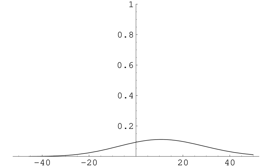
FIG. 1.: Example of propagation of gaussian wave-packet for particle of flavor $\alpha=1$ at $k_{0}\approx 0.35$GeV (time flow left-to-right and up-to-down). Here and in what follows the distance scale is GeV^-1.

FIG. 2.: Example of propagation of gaussian wave-packet for particle of flavor $\alpha=2$ at $k_{0}\approx 0.35$GeV (time flow left-to-right and up-to-down).

FIG. 3.: Two snapshots of distribution of flavor charge vs distance for originally well-localized wave-packet give an example of the coherence loss by a point-like flavor source. Also, clearly seen is EPR-correlated antiparticle wave-packet traveling in the opposite direction.

FIG. 4.: Example of field-theoretical fluctuations at the ”cross-over” time when particle of flavor $\alpha=1$ has been almost completely converted into flavor $\alpha=2$ (time flow left-to-right and up-to-down).

FIG. 5.: An example of tracking the position of maximum of the gaussian wave-packet. Position (y-axis) vs time (x-axis) is plotted and disruptions in numerical procedure caused by field-theoretical fluctuations are visible.

FIG. 6.: Space oscillations for particle (left) and antiparticle (right) populations (for flavor $\alpha=1$). ($k\approx 0.35$GeV)

FIG. 7.: Space oscillations for particle (left) and antiparticle (right) populations (for flavor $\alpha=2$). ($k\approx 0.35$GeV)

REFERENCES

• [1] Particle Data Group, R.M.Barnett et al., Phys. Rev.D54, 1 (1996).
• [2] H. Fritzsch, Z.Z. Xing hep-ph/0103242 (2001).
• [3] M. Czakon, J. Studnik, M. Zralek hep-ph/0006339 (2000).
• [4] J.H. Christenson et al, Phys. Rev. Lett. 13, 138 (1964).
• [5] M. Czakon, J. Studnik, M. Zralek, J. Gluza, hep-ph/0005167 (2000).
• [6] H. Fritzsch, Z.Z. Xing Prog. Part. Nucl. Phys. 45 (2000)1 ; hep-ph/9912358.
• [7] R. Mohapatra and P. Pal, ”Massive Neutrinos in Physics and Astrophysics,” World Scientific, Singapore, 1991; J.N. Bahcall, ”Neutrino Astrophysics,” Cambridge Univ. Press, Cambridge, UK, 1989; L. Oberauer and F. von Feilitzsch, Rep. Prog. Phys. 55 (1992), 1093; C.W. Kim and A. Pevsner, ”Neutrinos in Physics and Astrophysics,” Contemporary Concepts in Physics, Vol. 8, Harwood Academic, Chur, Switzerland, 1993.
• [8] N. Cabibbo, Phys. Rev. Lett. 10, 531 (1963).
• [9] For a recent theoretical overview, see C.-R. Ji and H.M. Choi, Nucl. Phys. B90, 93(2000).
• [10] M. Kobayashi and T. Maskawa, Prog. Theor. Phys. 49, 652 (1973).
• [11] L. Wolfenstein, Phys.Rev.Lett. 51, 1945 (1983).
• [12] K.C.Β Hannabuss and D.C.Β Latimer, J. Phys. A 36 (2003) L69; J. Phys. A. 33 (2000) 1369.
• [13] C.-R.Ji and Y.Mishchenko, Phys. Rev.D65, 096015 (2002).
• [14] M. Binger and C.-R. Ji, Phys. Rev. D 60, 056005 (1999).
• [15] C.-R. Ji and Y. Mishchenko, Phys. Rev. D 64, 076004 (2001); /hep-ph/0105094.
• [16] M. Blasone, A. Capolupo, O.Romei and G.Vitiello, hep-ph/0102048 (2001).
• [17] M. Blasone and G. Vitiello, Phys. Rev. D 60 (1999) 111302.
• [18] M. Blasone and G. Vitiello, Annals of Physics 244, 283-311 (1995).
• [19] M. Blasone, P.A. Henning and G. Vitiello, Phys. Lett. B 451, 140 (1999).
• [20] M. Blasone, A. Capolupo and G. Vitiello, hep-th/0107125 (2001).
• [21] M. Blasone, A. Capolupo and G. Vitiello, hep-ph/0107183 (2001).
• [22] K. Fujii, C. Habe and T. Yabuki, Phys. Rev. D59 (1999) 113003; hep-ph/9807266.
• [23] K. Fujii, C. Habe and T. Yabuki, Phys. Rev. D64 (2001) 013011.
• [24] C. Itzykson, J. Zuber ”Quantum Field Theory,” New York: McGraw-Hill Co., 1980.
• [25] N. Bogoliubov, D. Shirkov ”Introduction to the theory of quantized fields,” New York: John Wiley, 1980.
• [26] H.J.Lipkin, hep-ph/9901399; Phys. Lett.B348,604(1995).
• [27] M.Zralek, hep-ph/9810543.
• [28] C.Giunti and C.W.Kim, Found.Phys.Lett.14, 213 (2001).
• [29] M.Beuthe, Phys.Rev.D66, 013003 (2002);Phys. Rept.375, 105-218 (2003).
Refer to caption
Refer to caption
Refer to caption
Refer to caption
Refer to caption
Refer to caption