Nucleon form factors, $\boldsymbol{B}$-meson factories and the radiative return

Abstract

The feasibility of a measurement of the electric and magnetic nucleon form factors at $B$-meson factories through the radiative return is studied. Angular distributions allow a separation of the contributions from the two form factors. The distributions are presented for the laboratory and the hadronic rest frame, and the advantages of different coordinate systems are investigated. It is demonstrated that $Q^{2}$ values up to 8 or even 9 GeV² are within reach. The Monte Carlo event generator PHOKHARA is extended to nucleon final states, and results are presented which include Next-to-Leading Order radiative corrections from initial-state radiation. The impact of angular cuts on rates and distributions is investigated and the relative importance of radiative corrections is analysed.

1 Introduction

The importance of measuring the nucleon form factor has been repeatedly emphasized in the literature (e.g. iachello ; brodsky ; Baldini and refs therein). Recent experiments at Jefferson Lab have explored the ratio of electric and magnetic form factors in the space-like region JLab1 ; JLab2 up to  5.6 GeV², using the recoil polarization method; their results show disagreement with data obtained with the Rosenbluth method (For an extensive review see arrington . For recent suggestions of a possible explanation of this discrepancy through corrections from two-photon exchange see e.g. Guichon:2003qm ; Chen:2004tw .). Data in the time-like region based on electron–positron annihilation into proton–antiproton (and neutron–antineutron) final states, and the inverse reactions, only extend to 6 GeV² and 14 GeV² respectively. These latter measurements exhibit fairly large errors and do not provide a separation of the contributions from the two form factors. To explore the validity of the different model predictions, improved measurements over a wide kinematic range are desirable.

In the present paper the potential of the radiative return at $B$-meson factories will be explored. As shown below, these measurements will cover the region from threshold up to 8 or even 9 GeV² with sufficient counting rates. This region is also accessible at the Beijing storage ring and is complementary to the one at Cornell with energies above the $J/\psi$ resonance.

Not surprisingly, many aspects of the radiative return are quite similar to those of the reaction $e^{+}e^{-}\to p\bar{p}$. In particular it is again the square of the electric and magnetic form factors, which can be determined separately through the analysis of angular distributions.

Radiative corrections are indispensable for a precise interpretation of the data. Furthermore, given the limited acceptance and the asymmetric kinematic configuration at present $B$-meson factories, a Monte Carlo event generator is required to demonstrate the feasibility of the measurement. The present analysis is based on an extension of the generator PHOKHARA 3.0 Czyz:PH03 , which was originally constructed to simulate two-pion and two-muon Rodrigo:2001kf , and later four-pion Czyz:2002np ; Czyz:2000wh , production through the radiative return Binner:1999bt ; Zerwas and which includes next-to-leading order (NLO) radiative corrections Rodrigo:2001jr ; Kuhn:2002xg . The new version of PHOKHARA (PHOKHARA 4.0) will include, besides of the nucleon–antinucleon final states, final-state radiative corrections (FSR) to $\mu^{+}\mu^{-}$ production at NLO in_preparation .

For the present case we consider photon emission from the initial state only (ISR). As discussed below in more detail, final-state radiation is completely negligible if the reaction is considered at a centre of mass (cms) collider energy of 10.5 GeV.

The choice of form factors made by the program is directly taken from iachello ; ia-ja-la . It is, however, set up in a modular form such that the two form factors can be easily modified and replaced by the user, if required.

The program also allows a more detailed study of angular distributions, including the effects of cuts on photon and proton acceptance. Indeed we will find that these distributions are quite sensitive to the ratio of the form factors, and the extraction of this ratio seems to be feasible over a fairly large kinematic range.

2 Electric and magnetic form factors and the radiative return

The matrix element of the electromagnetic current governing nucleon–antinucleon production is conventionally written in terms of the Dirac ($F_{1}^{N}$) and Pauli ($F_{2}^{N}$) form factors

$$J_{\mu}=-ie\cdot\bar{u}(q_{2})\left(F_{1}^{N}(Q^{2})\gamma_{\mu}-\frac{F_{2}^{N}(Q^{2})}{4m_{N}}\left[\gamma_{\mu},Q/\ \right]\right)v(q_{1})~{},$$ (1)

where $N$ stands for proton or neutron. The nucleon and antinucleon momenta are denoted by $q_{1}$ and $q_{2}$ respectively, and $Q=q_{1}+q_{2}$.

Cross sections and distributions for $e^{+}e^{-}\to N\bar{N}$ are conveniently expressed in terms of the electric and magnetic Sachs form factors Sachs :

$$G_{M}^{N}=F_{1}^{N}+F_{2}^{N}~{},\qquad G_{E}^{N}=F_{1}^{N}+\tau F_{2}^{N}~{},$$ (2)

with $\tau=Q^{2}/4m^{2}_{N}$, which will also lead to compact formulae for the radiative return. Both proton and neutron form factors can be decomposed into isoscalar and isovector contributions (see e.g. ia-ja-la ):

$$F^{p}_{1,2}=F_{1,2}^{s}+F_{1,2}^{v}~{},\qquad F^{n}_{1,2}=F_{1,2}^{s}-F_{1,2}^{v}~{}.$$ (3)

Let us start with a qualitative discussion of form factor measurements through the radiative return, based on the leading order process

$$e^{+}(p_{1})+e^{-}(p_{2})\to\bar{N}(q_{1})+N(q_{2})+\gamma(k)~{}.$$ (4)

From the simple analytical results it will be straightforward to evaluate production rates, to understand the qualitative aspects of angular distributions, and to develop strategies for the separation of the electric and the magnetic form factor.

The differential cross section for reaction (4) (with ISR only) can be written as

$$d\sigma=\frac{1}{2s}L_{\mu\nu}H^{\mu\nu}d\Phi_{2}(p_{1}+p_{2};Q,k)d\Phi_{2}(Q;q_{1},q_{2})\frac{dQ^{2}}{2\pi}~{},$$ (5)

where $L_{\mu\nu}$ and $H^{\mu\nu}$ are the leptonic and hadronic tensors respectively. For notation, definitions and an explicit form of the leptonic tensor, see for instance Czyz:2000wh ; Kuhn:2002xg . The hadronic tensor is given by

$$H_{\mu\nu} = 2|G_{M}^{N}|^{2}(Q_{\mu}Q_{\nu}-g_{\mu\nu}Q^{2})$$ (6)

$$-\frac{8\tau}{\tau-1}\left(|G_{M}^{N}|^{2}-\frac{1}{\tau}|G_{E}^{N}|^{2}\right)q_{\mu}q_{\nu}~{},$$

where $q=(q_{2}-q_{1})/2$. From the explicit form of the hadronic tensor it becomes apparent that the relative phase between $G_{E}^{N}$ and $G_{M}^{N}$ cannot be measured in this experiment (i.e. as long as the spin of the nucleon remains unmeasured). This is independent of the detailed form of the leptonic tensor. In particular phases from higher order ISR or (longitudinal or transversal) beam polarization affect only the leptonic tensor and thus do not alter this conclusion.

Integrating over the whole range of nucleon angles and the photon azimuthal angle, and restricting the photon polar angle within $\frac{m_{e}}{\sqrt{s}}\ll\theta_{\gamma}^{\rm min}<\theta_{\gamma}<\pi-\theta_{\gamma}^{\rm min}$, the differential cross section factorizes into the cross section for electron–positron annihilation into hadrons and a flux factor that depends on $s$ and $Q^{2}$ only Binner:1999bt :

$$\frac{{\rm d}\sigma}{{\rm d}Q^{2}}=\frac{4\alpha^{3}}{3sQ^{2}}R(Q^{2})\biggl{\{}\frac{(1+\frac{Q^{4}}{s^{2}})}{(1-\frac{Q^{2}}{s})}\log\frac{1+c_{m}}{1-c_{m}}-\left(1-\frac{Q^{2}}{s}\right)c_{m}\biggl{\}}~{},$$ (7)

where $c_{m}=\cos\theta_{\gamma}^{\rm min}$, $m_{e}$ denotes the electron mass,

$$R(Q^{2})=\frac{\sigma(e^{+}e^{-}\rightarrow N\bar{N})}{\sigma_{\rm point}}=\frac{\beta_{N}}{2}\left(2|G_{M}^{N}|^{2}+\frac{1}{\tau}|G_{E}^{N}|^{2}\right)~{},$$ (8)

with $\sigma_{\rm point}$ the lowest order muonic cross section and $\beta_{N}^{2}=1-4m_{N}^{2}/Q^{2}$.

After integration over the whole range of nucleon angles, the separation of electric and magnetic form factors is no longer feasible. However, the modulus of their ratio can be determined from the study of properly chosen angular distributions. The fully differential cross section is essentially given by

$$L_{\mu\nu}H^{\mu\nu}=\frac{(4\pi\alpha)^{3}}{Q^{2}}\biggl{\{}\biggr{(}|G_{M}^{N}|^{2}-\frac{1}{\tau}|G_{E}^{N}|^{2}\biggr{)}$$ (9)

$$\kern 20.0pt\times\frac{32s}{\beta_{N}^{2}(s-Q^{2})}\biggr{(}\frac{1}{y_{1}}+\frac{1}{y_{2}}\biggr{)}\biggr{(}\frac{(p_{1}\cdot q)^{2}+(p_{2}\cdot q)^{2}}{s^{2}}\biggr{)}$$

$$+2\biggr{(}|G_{M}^{N}|^{2}+\frac{1}{\tau}|G_{E}^{N}|^{2}\biggr{)}\biggr{[}\biggr{(}\frac{1}{y_{1}}+\frac{1}{y_{2}}\biggr{)}\ \frac{(s^{2}+Q^{4})}{s(s-Q^{2})}-2\biggr{]}\biggl{\}}~{},$$

where $y_{1,2}=\frac{s-Q^{2}}{2s}(1\mp\cos\theta_{\gamma})$.

The separation of the form factors will therefore have to rely on the peculiar dependence of the differential cross section on the nucleon and antinucleon momenta separately.

The close connection between this analysis and the one based on the reaction $e^{+}e^{-}\to N\bar{N}$ becomes even more apparent once the result is expressed in terms of the polar and azimuthal angles $\hat{\theta}$ and $\hat{\varphi}$, which characterize the nucleon direction in the rest frame of the hadronic system, with the $z$-axis opposite to the direction of the real photon momentum and the $y$-axis in the plane spanned by the beam and the photon direction (see Appendix A):

$$L_{\mu\nu}H^{\mu\nu}=$$ (10)

$$=\frac{(4\pi\alpha)^{3}}{Q^{2}}\biggl{\{}\biggr{(}|G_{M}^{N}|^{2}-\frac{1}{\tau}|G_{E}^{N}|^{2}\biggr{)}\frac{4Q^{2}}{(s-Q^{2})}\biggr{(}\frac{1}{y_{1}}+\frac{1}{y_{2}}\biggr{)}$$

$$\phantom{00}\times\biggr{(}(\beta\gamma\cos\hat{\theta})^{2}+(\gamma\cos\theta_{\gamma}\cos\hat{\theta}-\sin\theta_{\gamma}\sin\hat{\theta}\sin\hat{\varphi})^{2}\Biggl{)}$$

$$+2\biggr{(}|G_{M}^{N}|^{2}+\frac{1}{\tau}|G_{E}^{N}|^{2}\biggr{)}\biggr{[}\biggr{(}\frac{1}{y_{1}}+\frac{1}{y_{2}}\biggr{)}\ \frac{(s^{2}+Q^{4})}{s(s-Q^{2})}-2\biggr{]}\biggl{\}}~{},$$

where $\gamma=(s+Q^{2})/2\sqrt{sQ^{2}}$ and $\beta=(s-Q^{2})/(s+Q^{2})$ characterize the boost from the laboratory to the hadronic rest frame. In the limit $Q^{2}\ll s$, this can be approximated by

$$L_{\mu\nu}H^{\mu\nu}= \frac{(4\pi\alpha)^{3}}{Q^{2}}\frac{(1+\cos^{2}\theta_{\gamma})}{(1-\cos^{2}\theta_{\gamma})}$$ (11)

$$\times 4\left(|G_{M}^{N}|^{2}(1+\cos^{2}\hat{\theta})+\frac{1}{\tau}|G_{E}^{N}|^{2}\sin^{2}\hat{\theta}\right)~{}.$$

An alternative choice of the coordinate system, which is obtained through an additional rotation around the $x$-axis in the hadronic rest frame, leads to a diagonal form of the leptonic tensor. In this frame the angular distribution of the baryons simplifies even further. This formulation is discussed in detail in the appendix. For small $Q^{2}/s$ the two frames nearly coincide.

It is instructive to compare the angular distribution in Eq. (11) with the angular distribution from $e^{+}e^{-}\to N\bar{N}$:

$$\frac{d\sigma}{d\Omega}=\frac{\alpha^{2}\beta_{N}}{4Q^{2}}\left(|G_{M}^{N}|^{2}(1+\cos^{2}\theta)+\frac{1}{\tau}|G_{E}^{N}|^{2}\sin^{2}\theta\right)~{}.$$ (12)

The close relation between Eqs. (11) and (12) is clearly visible.

As is already evident from the hadronic tensor in Eq. (6), the phases of the form factors are, however, not accessible by this method. Their determination would require the measurement of the polarization of the nucleons in the final state DDR ; Rock . PHOKHARA can easily be extended to describe this additional degree of freedom. This option is of particular interest for $\Lambda\bar{\Lambda}$ production, with its self-analysing decay mode.

As emphasized above, only ISR is included in the present version of the program. FSR with one photon only emitted from the hadronic system is described by the amplitude for $e^{+}e^{-}\to\gamma^{*}\to N\bar{N}\gamma$, with an invariant mass of the virtual photon of 10.5 GeV. This option is, however, strongly suppressed by the proton form factor. In fact, the arguments are quite similar to those for pion pair production, where FSR in leading order and at 10.5 GeV is completely negligible.

As will be discussed below, the event rate drops rapidly with increasing $Q^{2}$ and only few events will be observed for invariant hadron masses around 3 GeV. However, the rate for baryon pair production from $J/\psi$ decays will be significantly enhanced, all considerations given above for continuum production do apply, and a precise measurement of the branching ratio of $J/\psi$ into baryon pairs and the relative strength of magnetic and electric coupling is within reach.

3 Nucleon form factors and their implementation in PHOKHARA

The parametrization of the form factors used in this paper and listed below in detail is adopted from Ref. ia-ja-la , with the analytical continuation to the time-like region taken from iachello and brodsky . The isoscalar and isovector components of Dirac and Pauli form factors are given by:

$$F_{1}^{s}=\frac{g(Q^{2})}{2}\biggr{[}(1-\beta_{\omega}-\beta_{\phi})-\beta_{\omega}\cdot T_{\omega}-\beta_{\phi}\cdot T_{\phi}\biggr{]}~{},$$ (13)

$$F_{2}^{s}=\frac{g(Q^{2})}{2}\biggr{[}(0.120+\alpha_{\phi})\cdot T_{\omega}-\alpha_{\phi}\cdot T_{\phi}\biggr{]}~{},$$ (14)

$$F_{1}^{v}=\frac{g(Q^{2})}{2}\biggr{[}(1-\beta_{\rho})-\beta_{\rho}\cdot T_{\rho}\biggr{]}~{},$$ (15)

$$F_{2}^{v}=\frac{g(Q^{2})}{2}\biggr{[}-3.706\cdot T_{\rho}\biggr{]}~{},$$ (16)

with

$$T_{\rho}=\frac{m^{2}_{\rho}+8\Gamma_{\rho}m_{\pi}/\pi}{Q^{2}-m^{2}_{\rho}+(Q^{2}-4m^{2}_{\pi})\Gamma_{\rho}\alpha(Q^{2})/m_{\pi}}\ ,$$ (17)

$$\alpha(Q^{2})=\biggr{(}1-x^{2}\biggr{)}^{1/2}\biggl{\{}\frac{2}{\pi}\log\biggr{(}\frac{1+\sqrt{1-x^{2}}}{x}\biggr{)}-i\biggl{\}}\ ,$$ (18)

and

$$T_{\omega,\phi}=\frac{m^{2}_{\omega,\phi}}{Q^{2}-m^{2}_{\omega,\phi}}~{},\ g(Q^{2})=\frac{1}{(1-\gamma e^{i\theta}Q^{2})^{2}}~{},\ x=\frac{2m_{\pi}}{\sqrt{Q^{2}}}~{}.$$ (19)

The values of the parameters (dimensionful quantities in units of GeV) are $\beta_{\rho}=0.672$, $\beta_{\omega}=1.102$, $\beta_{\phi}=0.112$, $m_{\phi}=1.019$, $m_{\rho}=0.765$, $m_{\omega}=0.784$, $\alpha_{\phi}=-0.052$, $\Gamma_{\rho}=0.112$, $\gamma=0.25$. The angle $\theta$ in Eq. (19) is set to $\theta=\pi/4$ or $\theta=19\pi/64$ as recommended in iachello . More recent fits to the data in the space-like region are listed in gari_kru ; lomon . However, in view of the large uncertainty of the data the discrimination between the different parametrizations is not yet possible. It should be emphasized that the original fit of ia-ja-la agrees well with the ratio of the form factors measured at Jefferson Lab JLab1 ; JLab2 , as shown in Fig. 1. In the time-like region, the ratio of the form factors is predicted to increase with $Q^{2}$ (Fig. 2), in contrast to the behaviour in the space-like region.

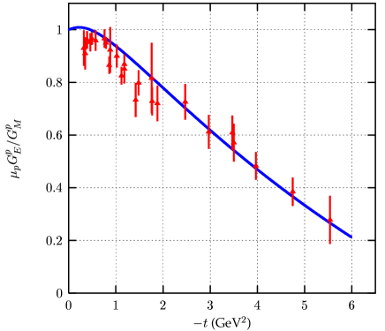
Figure 1: The ratio of proton form factors in the space-like region as predicted by the model ia-ja-la (solid line) and data from JLab JLab1 ; JLab2 . $\mu_{p}$ is the proton magnetic moment.

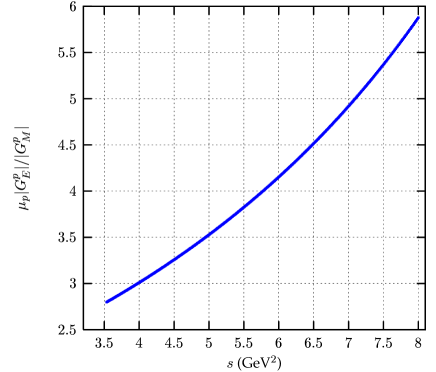
Figure 2: Modulus of the ratio of proton form factors in the time-like region as predicted by the model ia-ja-la .

Data giving information about the form factors in the time-like region originate from the reactions $e^{+}e^{-}\to p\bar{p}$, $p\bar{p}\to e^{+}e^{-}$ and $e^{+}e^{-}\to n\bar{n}$ and are shown in Figs. 3–5. Only measurements of the total cross section are available. Form factors, if available at all, are extracted under the assumption $G_{M}^{p}=\mu_{p}G_{E}^{p}$, and no true separation of the electric and magnetic form factors has been performed, a consequence of the low event rates. Within the large experimental uncertainties the data are in reasonable agreement with the model predictions. The poor experimental knowledge can be substantially improved by using the radiative return Binner:1999bt ; Zerwas at $B$-meson factories. Even the separation of electric and magnetic form factors may be envisaged in order to resolve the present discrepancies arrington in the measurement of the proton form factors.

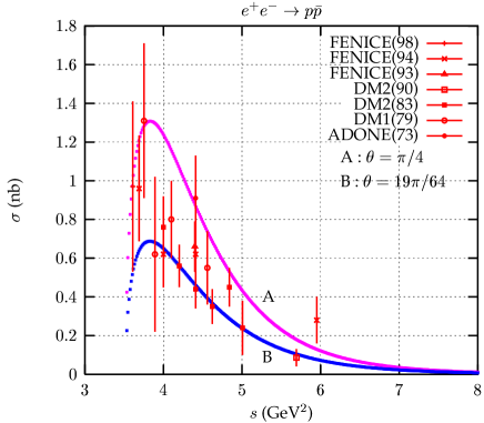
Figure 3: Comparison of the measured antonelli98 ; antonelli94 ; antonelli93 ; bisello90 ; bisello83 ; delcourt79 ; castellano73 $e^{+}e^{-}\to p\bar{p}$ cross section with the model from Ref. ia-ja-la . Predictions are given for two different values ($\pi/4$ - curve A and $19\pi/64$ - curve B) of the parameter $\theta$ (see Eq. (19)).

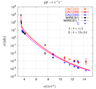
Figure 4: Comparison of the measured andreotti03 ; ambrogiani99 ; armstrong93 ; bardin91 ; bardin91a $p\bar{p}\to e^{+}e^{-}$ cross section with the model from Ref. ia-ja-la . Predictions are given for two different values ($\pi/4$ - curve A and $19\pi/64$ - curve B) of the parameter $\theta$ (see Eq. (19)). The curves were obtained without imposing any angular cuts. Theoretical results with cuts appropriate for each experiment are shown as crosses.

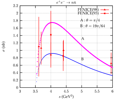
Figure 5: Comparison of the measured antonelli98 ; antonelli93 $e^{+}e^{-}\to n\bar{n}$ cross section with the model from Ref. ia-ja-la . Predictions are given for two different values ($\pi/4$ - curve A and $19\pi/64$ - curve B) of the parameter $\theta$ (see Eq. (19)).

The form factors defined in Eqs. (13)–(16) were implemented in the event generator PHOKHARA Czyz:2002np ; Czyz:PH03 ; Rodrigo:2001kf , providing a powerful tool for the experimental and theoretical analysis of the processes $e^{+}e^{-}\to p\bar{p}\gamma$ and $n\bar{n}\gamma$ at NLO. Real and virtual FSR contributions are not (yet) implemented. They might, however, become important in conjunction with hard ISR (lowering the effective $Q^{2}$) for $Q^{2}$ close to the $p\bar{p}$ threshold, where the final-state Coulomb interaction is sizeable.

The technical correctness of the implementation was checked first by confronting the $Q^{2}$ distribution of events generated by PHOKHARA 4.0 at LO with the corresponding analytical prediction in Eq. (7). The test was successfully performed with an agreement better than 0.1% for $Q^{2}<8$ GeV² (the region were the cross section is well accessible to experiment). At NLO the standard tests for the independence of the cross section on the ‘soft–hard’ separation parameter were performed again with a precision better than 0.1%. They guarantee that the implementation of the form factors in the one-photon and two-photon parts of the generator is consistent and, together with the LO test, support the correctness of the whole implementation.

4 Form factor measurements at $\boldsymbol{B}$-meson factories

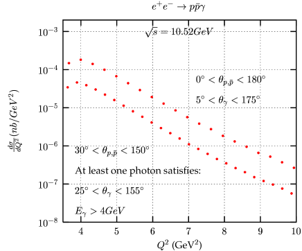
Figure 6: Differential cross section of the process $e^{+}e^{-}\to p\bar{p}\gamma(\gamma)$ for two different sets of cuts.

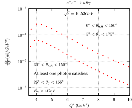
Figure 7: Differential cross section of the process $e^{+}e^{-}\to n\bar{n}\gamma(\gamma)$ for two different sets of cuts.

The differential cross section as a function of $Q^{2}$, as observed through the radiative return, is shown in Figs. 6 and 7. The upper curve represents the cross section after integration over all proton angles and over photon angles down to $5^{\circ}$ w.r.t. the beam direction. The lower curves are valid for cuts corresponding to the BaBar acceptance region transformed to the $e^{+}e^{-}$ cms. The cross sections corresponding to the lower curves, integrated over $Q^{2}<$ 10 GeV², amount to 59.3 fb for protons and to 125 fb for neutrons. With a luminosity of over 130 fb^-1 accumulated at $B$-factories already now, the event rate may be large enough to extract and separate $|G_{M}^{N}|$ and $|G_{E}^{N}|$ as proposed above.

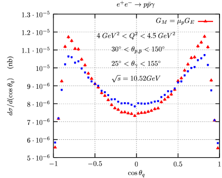
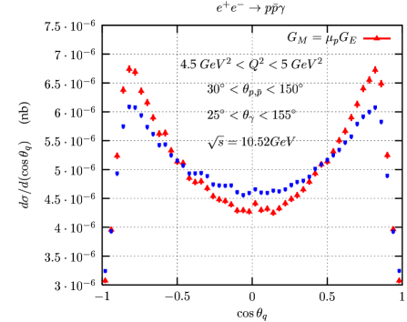
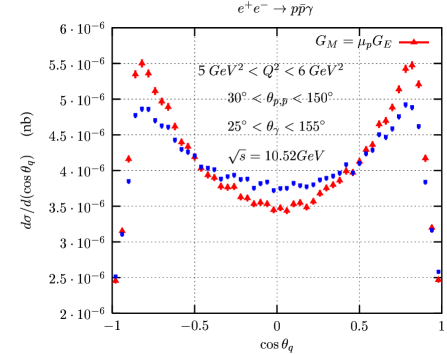
Figure 8: Angular distributions in the polar angle of vector ${\bf q}$ for three different ranges of $Q^{2}$, with and without the constraint $G_{M}^{p}=\mu_{p}G_{E}^{p}$ (see text for a more detailed explanation).

In Fig. 8 we show the angular distributions in $\theta_{q}$ (the polar angle of the vector ${\bf q}$) for different ranges of $Q^{2}$. To explore the sensitivity to the form factors individually we compare the differential cross sections obtained for the model described above with the distribution obtained under the assumption $G_{M}^{p}=\mu_{p}G_{E}^{p}$, subject, however, to the constraint that $\sigma(e^{+}e^{-}\rightarrow p\bar{p})$ (see Eq. (8)) remains unaffected. Without that constraint the predicted cross section would be up to ten times larger, in disagreement with existing data. The distributions are markedly different and the discrimination between different assumptions about the ratio $G_{M}^{p}/G_{E}^{p}$ seems feasible.

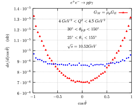
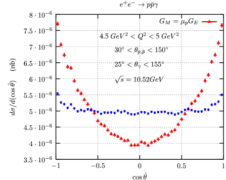
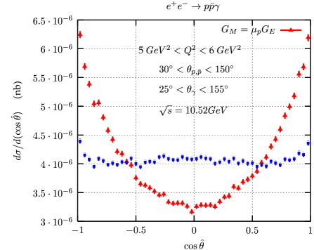
Figure 9: Angular distributions in the polar angle of the proton for three different ranges of $Q^{2}$, with and without the constraint $G_{M}^{p}=\mu_{p}G_{E}^{p}$ (see text for a more detailed explanation).

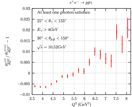
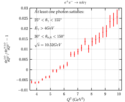
Figure 10: Comparison between LO and NLO predictions for the differential cross section of the reactions $e^{+}e^{-}\rightarrow p\bar{p}\gamma$ and $e^{+}e^{-}\rightarrow n\bar{n}\gamma$.

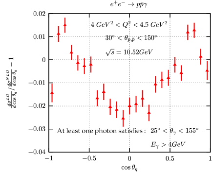
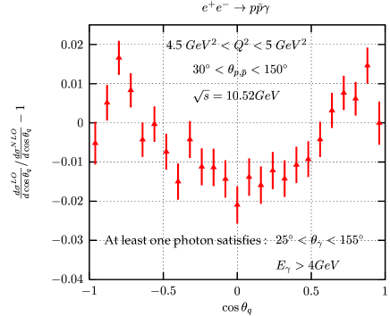
Figure 11: Comparison between LO and NLO predictions for the differential cross section of the reaction $e^{+}e^{-}\rightarrow p\bar{p}\gamma$ for two different ranges of $Q^{2}$.

The angular distribution of the baryons, if defined in the laboratory or cms frame, is strongly affected by the boost. The difference between different choices for the form-factor ratios is expected to be more pronounced for the proton angular distribution in the hadronic rest frame, with the $z$-axis aligned with the direction of the photon and the $y$-axis in the plane spanned by the beam and the photon directions (see Eqs. (10) and (11) above). In this case one may study alternatively the distributions with respect to $\hat{\theta}$ and $\hat{\varphi}$, the azimuthal and polar angles of the proton directions. For $Q^{2}\ll s$, the case relevant to the present discussion, the $\hat{\varphi}$ dependence is unimportant, and the pronounced dependence of the $\cos\hat{\theta}$ distribution on the choice of the form factors is clearly visible. The difference between the two model assumptions is significantly more pronounced, and the sensitivity to the form-factor ratio improves (Fig. 9).

A quantitative estimate of the precision of such a cross section measurement for proton production can be obtained from Fig. 6. As is evident from Eq. (7), the relative error in the distribution $d\sigma/dQ^{2}$ for a specific $Q^{2}$-interval is a direct measure of the relative error in $R(Q^{2})$, averaged over the same interval. Taking, for example, the angular cuts for photons and protons which roughly correspond to the detector acceptance, an integrated luminosity of $100~{}{\rm fb}^{-1}$ and a bin size of $0.5~{}\rm{GeV}^{2}$, one expects about 2500 / 600 / 250 events around 4 / 5 / 6 $\rm{GeV}^{2}$ and a resulting statistical precision of 2 / 4 / 6 %. For $1000~{}{\rm fb}^{-1}$ even 8 ${\rm GeV}^{2}$ could be reached, again with roughly 6% statistical precision. For neutrons the rates are even higher.

The sensitivity to the ratio $|G_{M}/(\mu G_{E})|$ can best be estimated from Fig. 9. Let us discuss the interval between 4.5 to 5 ${\rm GeV}^{2}$. We expect in total around 1000 events, and the discrimination between the two options shown in the Figure should be straightforward.

The importance of the radiative corrections can be deduced from Figs. 10 and 11. Even if the integrated cross sections are similar in LO and NLO (a difference below 0.5% is observed in both Figs. 10 and 11), the radiative corrections do lead to distortions of the distributions by 1–3%; furthermore, they depend on the details of the cuts and the criteria for event selection. Hence, the use of the NLO generator is highly recommended.

5 Summary

The radiative return at $B$-meson factories is well suited for measurements of the nucleon form factors over a wide kinematic range. It should be emphasized that these measurements of the proton and neutron form factors can be obtained from the data sample taken in standard runs and close to the $\Upsilon$-resonance. Valid for the time-like region, they would complement the precise results for the space-like region from JLab. Close to the threshold the statistical precision would be at the per cent level, and eventually, depending on the integrated luminosity, these measurements could extend out to 8 or even 9 ${\rm GeV}^{2}$.

In order to demonstrate the feasibility of the method for realistic cuts, the Monte Carlo event generator PHOKHARA has been extended to simulate this reaction for $p\bar{p}\gamma$ and $n\bar{n}\gamma$ final states. Examples for event rates and for angular distributions have been presented, which include realistic cuts and which demonstrate the feasibility of these measurements. NLO corrections to ISR amount to typically 1–3%. They are part of the present event generator and should be included in a realistic simulation.

Angular distributions allow the separation of electric and magnetic form factors. The general form of these distributions has been studied. They become relatively simple in the hadronic rest frame, with the $z$-axis aligned with the photon direction. For a specific (“optimal”) orientation of the $z$-axis the leptonic tensor can even be diagonalized, which leads to a particularly simple form for the angular distribution. In fact, this form is quite similar to the one observed in the direct electron-positron annihilation reaction. The simulation also demonstrates that the separation of the squares of electric and magnetic form factors, respectively, can be achieved over a fairly wide $Q^{2}$-range, even if realistic acceptance cuts are imposed. To get access to the relative phase between electric and magnetic form factors, the determination of the nucleon spin is required, which is an attractive option for $\Lambda\bar{\Lambda}$ production. We will come back to this possibility in a subsequent study.

Appendix A The diagonal leptonic tensor

Let us start with the leptonic tensor (see e.g. Kuhn:2002xg , Eq. (4)) in the limit $m_{e}^{2}\ll s$ and $m_{e}^{2}/s\ll\theta^{2}_{\gamma}$:

$$L^{\mu\nu} = \frac{(4\pi\alpha)^{2}}{Q^{4}y_{1}y_{2}}\biggl{[}-\left(2\frac{Q^{2}}{s}+y_{1}^{2}+y_{2}^{2}\right)g^{\mu\nu}$$ (20)

$$-\frac{4Q^{2}}{s^{2}}(p^{\mu}_{1}p^{\nu}_{1}+p^{\mu}_{2}p^{\nu}_{2})\biggr{]}$$

where $y_{1,2}=\frac{s-Q^{2}}{2s}(1\mp\cos\theta_{\gamma})$.

Terms proportional to $Q_{\mu}$ and $Q_{\nu}$ do not contribute as a consequence of current conservation, $Q_{\mu}J^{\mu}_{\mathrm{had}}=0$, and have been dropped. The momenta in the laboratory frame, with the $z$-axis pointing along the positron beam are given by

$$p_{1,2}^{\mu}=\frac{\sqrt{s}}{2}\left(\begin{array}[]{c}1\\ 0\\ 0\\ \pm 1\end{array}\right),\;\;\;k^{\mu}=\frac{s-Q^{2}}{2\sqrt{s}}\left(\begin{array}[]{c}1\\ 0\\ s_{\gamma}\\ c_{\gamma}\end{array}\right),$$

$$Q^{\mu}=\frac{s-Q^{2}}{2\sqrt{s}}\left(\begin{array}[]{c}\frac{s+Q^{2}}{s-Q^{2}}\\ 0\\ -s_{\gamma}\\ -c_{\gamma}\end{array}\right),$$ (21)

with $s_{\gamma}=\sin\theta_{\gamma}$ and $c_{\gamma}=\cos\theta_{\gamma}$ accordingly. We perform the following transformations: a rotation of the coordinate frame around the $x$-axis, such that the new $z$-axis points into the negative photon direction and subsequent boost from the laboratory frame along the new $z$-axis with $\gamma\equiv(s+Q^{2})/2\sqrt{sQ^{2}}$ into the hadron rest frame. Then, one finds

$$p_{1,2}^{\mu}=\frac{\sqrt{s}}{2}\gamma\left(\begin{array}[]{c}(1\pm\beta c_{\gamma})\\ 0\\ \pm s_{\gamma}/\gamma\\ (-\beta\mp c_{\gamma})\end{array}\right),\;\;\;\;q^{\mu}=\frac{\sqrt{Q^{2}}}{2}\beta_{N}\left(\begin{array}[]{c}0\\ s_{\hat{\theta}}c_{\hat{\varphi}}\\ s_{\hat{\theta}}s_{\hat{\varphi}}\\ c_{\hat{\theta}}\end{array}\right),$$

$$Q^{\mu}=\sqrt{Q^{2}}\left(\begin{array}[]{c}1\\ 0\\ 0\\ 0\end{array}\right).$$ (22)

In this coordinate system the space components of the leptonic tensor are given by

$$L^{ij} = \frac{(4\pi\alpha)^{2}}{Q^{4}y_{1}y_{2}}\biggl{[}\left(2\frac{Q^{2}}{s}+y_{1}^{2}+y_{2}^{2}\right)\delta^{ij}$$ (23)

$$-\frac{Q^{2}}{s}\gamma^{2}(v^{i}_{1}v^{j}_{1}+v^{i}_{2}v^{j}_{2})\biggr{]}~{},$$

with

$$\vec{v}_{1,2}=\left(\begin{array}[]{c}0\\ \pm s_{\gamma}/\gamma\\ (-\beta\mp c_{\gamma})\end{array}\right).$$ (24)

In combination with the hadronic tensor this leads immediately to Eq. (10). The leptonic tensor, as given above, is evidently symmetric. The combination

$$(v^{i}_{1}v^{j}_{1}+v^{i}_{2}v^{j}_{2})/2=\left(\begin{array}[]{lll}0\phantom{000}&0&0\\ 0&s^{2}_{\gamma}/\gamma^{2}&-s_{\gamma}c_{\gamma}/\gamma\\ 0&-s_{\gamma}c_{\gamma}/\gamma\phantom{0}&(\beta^{2}+c_{\gamma}^{2})\\ \end{array}\right)$$ (25)

can thus be diagonalized by a rotation of the coordinate system around the $x$-axis, now, however, in the hadron rest frame. The rotation angle $\theta_{D}$ is obtained from

$$\tan\theta_{D}=\sqrt{\frac{\lambda-a}{\lambda+a}}=\frac{\gamma(\lambda-a)}{2s_{\gamma}c_{\gamma}},$$ (26)

or, alternatively

$$\tan(2\theta_{D})=\frac{2s_{\gamma}c_{\gamma}}{\gamma a}$$ (27)

where

$$\lambda=\lambda(\beta^{2},-c^{2}_{\gamma},s^{2}_{\gamma}/\gamma^{2});\;\;\;\;a=(\beta^{2}+c^{2}_{\gamma}-s^{2}_{\gamma}/\gamma^{2}),$$ (28)

with

$$\lambda(x,y,z)=\sqrt{x^{2}+y^{2}+z^{2}-2(xy+xz+yz)}.$$ (29)

The eigenvalues of $(v^{i}_{1}v^{j}_{1}+v^{i}_{2}v^{j}_{2})/2$ are given by

$$\lambda_{\pm}=(\beta^{2}+c^{2}_{\gamma}+s^{2}_{\gamma}/\gamma^{2}\pm\lambda)/2$$ (30)

and the leptonic tensor in the new “optimal” frame simplifies to

$$L^{ij} = \frac{(4\pi\alpha)^{2}}{Q^{4}y_{1}y_{2}}\biggl{[}\left(2\frac{Q^{2}}{s}+y_{1}^{2}+y_{2}^{2}\right)\delta^{ij}$$ (31)

$$-2\frac{Q^{2}}{s}\gamma^{2}\mbox{\rm diag}(0,\lambda_{-},\lambda_{+})\biggr{]}~{}.$$

Choosing this new “optimal” frame for the definition of the baryon direction with angles denoted by $\tilde{\theta}$ and $\tilde{\varphi}$, only quadratic terms in $\cos\tilde{\theta}$ and $\sin\tilde{\theta}\sin\tilde{\varphi}$ remain in the angular distribution. The combination $L_{ij}H^{ij}$ is now given by

$$L^{ij}H_{ij}=\frac{(4\pi\alpha)^{2}}{Q^{2}y_{1}y_{2}}\biggl{[}(2\frac{Q^{2}}{s}+y_{1}^{2}+y_{2}^{2})(3A+\beta_{N}^{2}B)-2\frac{Q^{2}}{s}\gamma^{2}$$

$$\times\biggl{(}A(\lambda_{+}+\lambda_{-})+\beta^{2}_{N}B(\lambda_{-}\sin^{2}\tilde{\theta}\sin^{2}\tilde{\varphi}+\lambda_{+}\cos^{2}\tilde{\theta})\biggr{)}\biggr{]}~{},$$

where $A$ and $B$ characterize the hadronic tensor

$$H_{\mu\nu} = A(Q_{\mu}Q_{\nu}-g_{\mu\nu}Q^{2})+4Bq_{\mu}q_{\nu}\ .$$ (33)

For two-particle production this is the most general form of the symmetric hadronic tensor, if one sums over polarizations of the particles in the final state. For the nucleon–antinucleon final state specifically, one finds

$$\kern-10.0ptA=2|G_{M}^{N}|^{2}\ \ {\rm and}\ \ B=-\frac{2\tau}{\tau-1}\left(|G_{M}^{N}|^{2}-\frac{1}{\tau}|G_{E}^{N}|^{2}\right).$$ (34)

Let us emphasize that this choice of coordinates also leads to an extremely simple angular distribution for pion pairs, and quite generally for any single-particle inclusive distribution.

In the the limit of $Q^{2}\ll s$ the rotation angle $\theta_{D}$ vanishes, the direction of the photon can be used as (negative) $z$-axis and the leptonic tensor reduces to

$$L^{ij}=\frac{(4\pi\alpha)^{2}}{Q^{4}y_{1}y_{2}}\frac{(1+c_{\gamma}^{2})}{2}\mbox{\rm diag}(1,1,0)~{},$$ (35)

and

$$L^{ij}H_{ij}\simeq\frac{(4\pi\alpha)^{2}}{Q^{2}y_{1}y_{2}}\left(1+c_{\gamma}^{2}\right)\left[2A+B\beta^{2}_{N}\sin^{2}\tilde{\theta}\right]\ ,$$ (36)

which for $A$ and $B$ from Eq. (34) gives

$$\kern-30.0ptL^{ij}H_{ij}\simeq\frac{(4\pi\alpha)^{2}}{Q^{2}y_{1}y_{2}}\left(1+c_{\gamma}^{2}\right)$$

$$\times\left[|G_{M}^{N}|^{2}\left(1+\cos^{2}\tilde{\theta}\right)+\frac{1}{\tau}|G_{E}^{N}|^{2}\sin^{2}\tilde{\theta}\right]\$$ (37)

which is closely related to Eq. (12).

References

- (1) F. Iachello, nucl-th/0312074 and talk at Workshop on in the 1–2 GeV range: Physics and Accelerator Prospects, Alghero, Sardinia (Italy), 10-13 September, 2003.
- (2) S. J. Brodsky, C. E. Carlson, J. R. Hiller and D. S. Hwang, [hep-ph/0310277]
- (3) Baldini, R. et al., eConf C010430 (2001) T20 [hep-ph/0106006]; Eur. Phys. J. C11 (1999) 709.
- (4) O. Gayou et al. Phys. Rev. Lett. 88 (2002) 092301 [nucl-ex/0111010]; Phys. Rev. C 64 (2001) 038202.
- (5) M. K. Jones et al. Phys. Rev. Lett. 84 (2000) 1398 [nucl-ex/9910005].
- (6) J. Arrington, Phys. Rev. C 68 (2003) 034325 [nucl-ex/0305009].
- (7) P. A. M. Guichon and M. Vanderhaeghen, Phys. Rev. Lett. 91 (2003) 142303 [hep-ph/0306007].
- (8) Y. C. Chen, A. Afanasev, S. J. Brodsky, C. E. Carlson and M. Vanderhaeghen, hep-ph/0403058.
- (9) H. Czyż, A. Grzelińska, J. H. Kühn and G. Rodrigo, hep-ph/0308312 (to appear in Eur. Phys. J. C).
- (10) G. Rodrigo, H. Czyż, J.H. Kühn and M. Szopa, Eur. Phys. J. C 24 (2002) 71 [hep-ph/0112184].
- (11) H. Czyż, A. Grzelińska, J. H. Kühn and G. Rodrigo, Eur. Phys. J. C 27 (2003) 563 [hep-ph/0212225].
- (12) H. Czyż and J. H. Kühn, Eur. Phys. J. C 18 (2001) 497 [hep-ph/0008262].
- (13) S. Binner, J. H. Kühn and K. Melnikov, Phys. Lett. B 459 (1999) 279 [hep-ph/9902399].
- (14) Min-Shih Chen and P. M. Zerwas, Phys. Rev. D 11 (1975) 58.
- (15) G. Rodrigo, A. Gehrmann-De Ridder, M. Guilleaume and J. H. Kühn, Eur. Phys. J. C 22 (2001) 81 [hep-ph/0106132].
- (16) J. H. Kühn and G. Rodrigo, Eur. Phys. J. C 25 (2002) 215 [hep-ph/0204283].
- (17) H. Czyż, A. Grzelińska, J. H. Kühn and G. Rodrigo, in preparation.
- (18) F. Iachello, A. D. Jackson and A. Lande, Phys. Lett. B 43 (1973) 191.
- (19) R.G. Sachs, Phys. Rev. 126 (1962) 2256; J. D. Walecka, Nuovo Cim. 11 (1959) 821.
- (20) A. Z. Dubnickova, S. Dubnicka and M. P. Rekalo, Nuovo Cim. A109 (1996) 241.
- (21) S. Rock, eConf C010430 (2001) W14 [hep-ex/0106084].
- (22) M. Gari, W. Krumpelmann Phys. Lett. B 173 (1986) 10; Z. Phys. A 322 (1985) 689.
- (23) E. L. Lomon, Phys. Rev. C 66 (2002) 045501 [nucl-th/0203081]; Phys. Rev. C 64 (2001) 035204 [nucl-th/0104039].
- (24) A. Antonelli et al. (FENICE collaboration), Nucl. Phys. B517 (1998) 3.
- (25) A. Antonelli et al. (FENICE collaboration), Phys. Lett. B 334 (1994) 431.
- (26) A. Antonelli et al. (FENICE collaboration), Phys. Lett. B 313 (1993) 283.
- (27) D. Bisello et al. (DM2 collaboration), Z. Phys. C48 (1990) 23.
- (28) D. Bisello et al. (DM2 collaboration), Nucl. Phys. B224 (1983) 379.
- (29) B. Delcourt et al. (DM1 collaboration), Phys. Lett. B 86 (1979) 395.
- (30) M. Castellano et al. (ADONE collaboration), Nouvo Cim. 14A (1973) 1.
- (31) M. Andreotti et al. (CALO collaboration), Phys. Lett.B 559 (2003) 20.
- (32) M. Ambrogiani et al. (CALO collaboration), Phys. Rev. D60 (1999) 032002.
- (33) T. A. Armstrong et al. (CALO collaboration), Phys. Rev. Lett.70 (1993) 1212.
- (34) G. Bardin et al. (WIRE collaboration), Phys. Lett. B 257 (1991) 514.
- (35) G. Bardin et al. (WIRE collaboration), Phys. Lett.B 255 (1991) 149.