A COMPARISON OF PREDICTIONS FOR SM HIGGS BOSON PRODUCTION AT THE LHC

1 INTRODUCTION

The dominant mechanism for the production of a SM Higgs boson at the LHC is gluon-gluon fusion through a heavy (top) quark loop. For this reason this channel has attracted a large amount of theoretical attention [1]. Recently, the total cross section has been calculated to NNLO in the strong coupling constant $\alpha_{s}$ (i.e. at order ${\cal O}(\alpha_{s}^{4})$) [2, 3, 4, 5, 6] and also contributions from multiple soft gluon emission have been consistently included to NNLL accuracy [7]. In addition to the size of the total rate, a knowledge of the shape of the Higgs boson $p_{T}$ distribution is essential for any search and analysis strategies at the LHC. In particular, the $p_{T}$ distribution for the Higgs boson is expected to be harder than the one of its corresponding backgrounds. The Higgs boson $p_{T}$ distribution has been computed with LL parton shower Monte Carlos (HERWIG [8] and PYTHIA [9]), and through various resummed calculations. The latter techniques are the more powerful ones, but it is primarily the former that experimentalists at the LHC have to rely upon, because of their flexibility in allowing to test the effects of the various kinematic cuts which may optimize search strategies.

In the kinematic region $p_{T}^{2}\ll m_{H}^{2}$, where most of the events are expected, large logarithmic corrections appear of the form $\alpha_{s}^{n}\ln^{m}m_{H}^{2}/p_{T}^{2}$ that spoil the validity of the fixed order perturbative expansion. The $p_{T}$ distribution can be written as

$$\frac{d\sigma}{dp_{T}^{2}}=\frac{d\sigma^{\rm res.}}{dp_{T}^{2}}+\frac{d\sigma^{\rm fin.}}{dp_{T}^{2}}\,.$$ (1)

The first term contains all logarithmically-enhanced contributions and requires their resummation to all orders. The second term is free from logarithmically-enhanced contributions and can be evaluated at fixed order in perturbation theory. The method to perform the all-order resummation is well known: to correctly take into account momentum conservation the resummation must be performed in the impact parameter ($b$) space [10, 11]. The large logarithmic contributions are exponentiated in the Sudakov form factor, which in the CSS [12] approach takes the form

$$S_{c}=\int_{b_{0}^{2}/b^{2}}^{m_{H}^{2}}\frac{d\mu^{2}}{\mu^{2}}\left[A_{c}\left(\alpha_{s}(\mu)\right)\ln\left(\frac{m_{H}^{2}}{\mu^{2}}\right)+B_{c}\left(\alpha_{s}(\mu)\right)\right],$$ (2)

where $b_{0}=2e^{-\gamma}$ and $c=q,g$. The $A_{c}$ and $B_{c}$ functions are free of large logarithmic corrections and can be computed as expansions in the strong coupling constant $\alpha_{s}$:

$$A_{c}(\alpha_{s})= \sum_{n=1}^{\infty}\left(\frac{\alpha_{s}}{\pi}\right)^{n}A_{c}^{(n)},$$ (3)

$$B_{c}(\alpha_{s})= \sum_{n=1}^{\infty}\left(\frac{\alpha_{s}}{\pi}\right)^{n}B_{c}^{(n)}.$$ (4)

The functions $A_{c}$ and $B_{c}$ control soft and flavour-conserving collinear radiation at scales $1/b\raisebox{-1.72218pt}{\hbox to0.0pt{$\,\sim\,$\hss}}\raisebox{1.72218pt}{$\,<\,$}\mu\raisebox{-1.72218pt}{\hbox to0.0pt{$\,\sim\,$\hss}}\raisebox{1.72218pt}{$\,<\,$}m_{H}$. Purely soft radiation at a very low scales $\mu\raisebox{-1.72218pt}{\hbox to0.0pt{$\,\sim\,$\hss}}\raisebox{1.72218pt}{$\,<\,$}1/b$ cancels out because the cross section is infrared safe and only purely collinear radiation up a scale $\mu\sim 1/b$ remains, which is taken into account by the coefficients

$$C_{ab}(\alpha_{s},z)=\sum_{n=1}^{\infty}\left(\frac{\alpha_{S}}{\pi}\right)^{n}C_{ab}^{(n)}(\alpha_{s},z).$$ (5)

Beyond NLL accuracy, to preserve the process independence of the resummation formula, an additional (process dependent) coefficient $H$ is needed [13], which accounts for hard virtual corrections and has an expansion

$$H_{c}(\alpha_{s})=1+\sum_{n=1}^{\infty}\left(\frac{\alpha_{s}}{\pi}\right)^{n}H_{c}^{(n)}.$$ (6)

In the case of Higgs boson production through $gg$ fusion, the relevant coefficients $A_{g}^{(1)}$, $A_{g}^{(2)}$ and $B_{g}^{(1)}$ are known [14] and control the resummation up to NLL accuracy . The NNLL coefficients $C^{(1)}_{ab}$ and $H_{g}^{(1)}$ are also known [16, 13]. The NNLL coefficient $B_{g}^{(2)}$ has been computed in Refs. [17, 18], whereas $A_{g}^{(3)}$ is not yet known exactly. In the following we assume that its value is the same that appears in threshold resummation [19].

2 PREDICTIONS FOR $p_{T}$ SPECTRA AND COMPARISONS

In the 1999 Les Houches workshop, a comparison [20, 21] of the HERWIG and PYTHIA (2 versions) predictions for the Higgs boson $p_{T}$ distribution with those of a $p_{T}$ resummation program (ResBos [22, 23]) was carried out. This comparison was continued in the 2001 workshop and examined the impact of the $B^{(2)}$ coefficient  [1]. In the meantime, a number of new theoretical predictions have become available, both from resummation and from the interface of NLO calculations with parton shower Monte Carlos. For these proceedings, we have carried out a comparison of most of the available predictions for the Higgs boson $p_{T}$ distribution at the LHC. We have used a Higgs boson mass of 125 GeV and either the MRST2001 or the CTEQ5M pdf’s. The difference between the two pdf’s for the production of a 125 GeV mass Higgs boson is of the order of a few percent. Before comparing the different predictions, we comment on the various approaches in turn.

Parton shower MC programs such as HERWIG, which implements angular ordering exactly, implicitly include the $A^{(1)}$, $A^{(2)}$ and $B^{(1)}$ coefficients and thus correctly sum the LL and part of the N^kLL contributions. However, in the most straightforward implementations, MC cannot correctly treat hard radiation. By contrast, the PYTHIA MC, which does not provide an exact implementation of angular ordering, has a hard matrix element correction . Recently, an approach to match NLO calculations to parton showers generators, MC@NLO [25, 26], has been proposed, and applied, amongst the other, to Higgs production. This method joins the virtues of NLO parton level generators (correct treatment of hard radiation, exact NLO normalization) to the ones of MC. It thus can be compared to a resummed calculation at NLL+NLO accuracy.

As far as resummed calculations are concerned, we first consider two implementation of the CSS approach. The ResBos code includes the $A_{c}^{(1,2,3)}$, $B_{c}^{(1,2)}$ and $C_{ab}^{(1)}$ coefficients in the low-$p_{T}$ region and matches this to the NLO distribution at high $p_{T}$. NNLO effects at high $p_{T}$ are approximately taken into account by scaling the second term in Eq. (1) with a K-factor. The matching is performed through a switching procedure whose uncertainty will be considered in the following. The calculation of Berger and Qiu [27] also performs a $p_{T}$ resummation in $b$ space and is accurate to NLL. The coefficient $B^{(2)}$ is included but the matching is still to NLO. Note that in both these approaches the integral of the spectrum is affected by higher-order contributions included in a non-systematic manner whose effect is not negligible for Higgs production.

The prediction by Bozzi, Catani, de Florian and Grazzini [28] (labeled Grazzini et al. in the following) is based on an implementation of the $b$-space formalism described in [13, 28]. The calculation has the highest nominal accuracy since it matches NNLL resummation at small $p_{T}$ to the NNLO result at high $p_{T}$[29]. This approach includes the coefficients $C_{ab}^{(2)}$ and $H_{g}^{(2)}$ in approximated form. The main differences with respect to the standard CSS approach are the following. A unitarity constraint is imposed, such that the total cross section at the nominal (NNLO) accuracy is exactly recovered upon integration. A study of uncertainties from missing higher order contributions can be performed as it is normally done in fixed order calculations, that is, by varying renormalization and factorization scales around the central value, that is chosen to be $m_{H}$.

Finally, we discuss the $p_{T}$ distribution of Ref. [30] (Kulesza et al.). This is obtained using a joint resummation formalism, by which both threshold and low-$p_{T}$ logarithmic contributions are resummed to all orders. This approach has been formally developed to NLL accuracy, but the NNLL coefficients $A^{(3)},B^{(2)},C^{(1)}$ and $H^{(1)}$ can also be incorporated. The matching is still performed to NLO. Even though a low mass Higgs boson at the LHC is produced with relatively low $x$ partons, threshold effects can still be significant due to the large color charge in the $gg$ initial state as well as steep $x$ dependence of the gluon distribution functions at low $x$. This leads to an increased sensitivity to Sudakov logarithms associated with partonic threshold for gluon-induced processes, as shown in Ref. [7].

It is known that the low-$p_{T}$ region is sensitive to non-perturbative effects. These are expected to be less important in the gluon channel due to the larger colour charge of the $gg$ initial state [21]. Different treatments of non-perturbative effects are included in the ResBos, Berger et al. and Kulesza et al calculation, whereas Grazzini et al. prediction is purely perturbative.

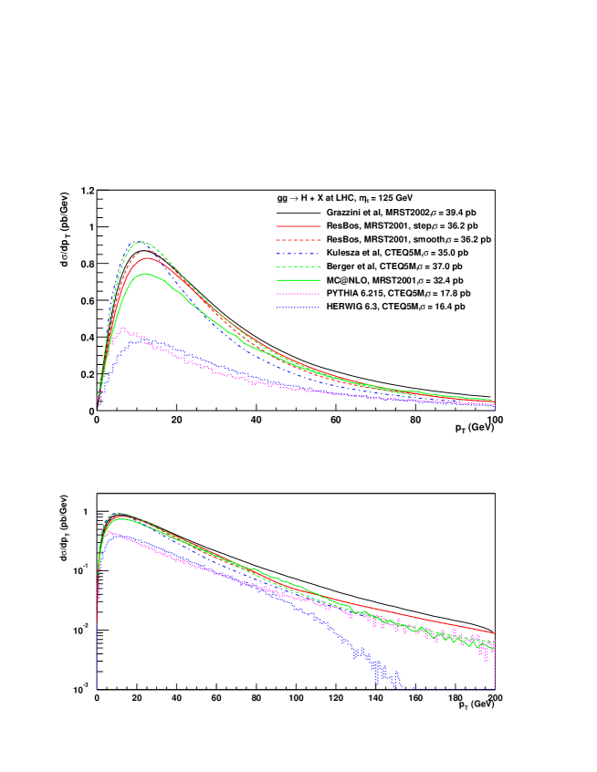
Figure 1: The absolute predictions for the production of a 125 GeV mass Higgs boson at the LHC.

The absolute predictions for the cross sections are shown in Figure 1. All curves are obtained in the $m_{\rm top}\to\infty$ limit. HERWIG and PYTHIA cross sections are significantly smaller than the other predictions, their normalization being fixed to LO. In the high-$p_{T}$ region, the HERWIG prediction drops quickly due to the lack of hard matrix element corrections. PYTHIA, in contrast, features the hard matrix element corrections. We also note that PYTHIA prediction is significantly softer than all the other curves, and thus its overall shape is fairly different from all the other predictions.

The MC@NLO cross section, about 32.4 pb, is roughly twice that of the HERWIG and PYTHIA predictions, being fixed to the NLO total cross section.

Two predictions (step, smooth) are shown for ResBos which differ in the manner in which the matching at high $p_{T}$ is performed. Their difference can be considered as an estimate of the ambiguity in the switching procedure. The two curves correspond to the same total cross section of about 36.2 pb, which is about 8 % higher than the NLO cross section. This is the effect of the higher-order terms that enter the prediction for the total rate in the context of the CSS approach. A slightly softer curve is obtained by Berger and Qiu. The predicted cross section (37 pb) is close to that of ResBos.

The Grazzini et al. prediction has an integral of about 39.4 pb, which corresponds to the total cross section at NNLO. Contrary to what is done in Ref. [28], here the curve is obtained with MRST2002 NNLO partons and three-loop $\alpha_{s}$. The difference with the result obtained with MRST2001 NNLO PDFs is completely negligible.

Concerning the Kulesza et al curve, the subleading terms associated with low $x$ emission (i.e. in the limit opposite to partonic threshold) and of which only a subset is included in the joint resummation formalism, play an important role numerically. As a result, the total cross section turns out to be 35 pb, about $10\%$ lower than the pure threshold result, which is 39.4 pb [30].

We now want to examine in more detail the relative shapes of the predictions plotted in Figure. 1. In Figure. 2 all the predictions are normalized to the Grazzini et al. cross section of 39.4 pb.

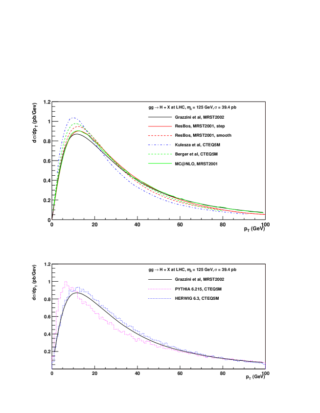
Figure 2: The predictions for the production of a 125 GeV mass Higgs boson at the LHC, all normalized to the same cross section for better shape comparison.

In the region of small and moderate $p_{T}$ (say, smaller than 100 GeV) all of the predictions are basically consistent with each other, with the notable exception of PYTHIA, which predicts a much softer spectrum. The curve of Kulesza et al. is also softer than the others.

For larger $p_{T}$, HERWIG gives unreliable predictions, since the transverse momentum is generated solely by means of the parton shower, and therefore it lacks hard matrix element effects. The Grazzini et al. and ResBos curves are harder than MC@NLO for large $p_{T}$. There are two reasons for this. Grazzini et al. implement the NNLO matrix elements exactly, corresponding to the emission of two real partons accompanying the Higgs in the final state [29]; ResBos mimics these contributions, by multiplying the NLO matrix elements by the K factor. MC@NLO, on the other hand, contains only NLO matrix elements (one real parton in the final state). Secondly, Grazzini et al. and ResBos choose the renormalization and factorization scales equal to $m_{H}$, whereas in MC@NLO these scales are set equal to the transverse mass of the Higgs, $\sqrt{m_{H}^{2}+p_{T}^{2}}$. The difference is small at the level of total rates, but it is not negligible in the tail of the $p_{T}$ distribution.

3 CONCLUSIONS

Up to now, the ATLAS and CMS experiments have relied primarily on the predictions from HERWIG and PYTHIA in designing both their experiments as well as defining their search and analysis strategies. In the last few years, a number of tools for and predictions of the Higgs boson cross section at the LHC have become available, with the inclusion of beyond-the-leading-order effects at different level of accuracy. In the case of total rates, NNLO results have recently become available; their consistent inclusion in experimental analysis will allow to further decrease the estimated lower bound on the integrated luminosity to be collected for discovery.

In this contribution, we primarily focused on the predictions for the $p_{T}$ spectrum, comparing the results of Monte Carlos with those obtained with analytically-resummed calculations. In contrast to the situation in 1999, all of the predictions, with the exception of PYTHIA, result in the same general features, most notably in the position of the peak. However, differences do arise, because of different treatments of the higher orders. It is an interesting question beyond the scope of this review that of whether these differences are resolvable at the experimental level, which may lead to modify the strategy for searches. In order to answer this, studies including realistic experimental cuts must be performed with the newly available tools.

References

- [1] D. Cavalli et al. 2002.
- [2] S. Catani, D. de Florian, and M. Grazzini. JHEP, 05:025, 2001.
- [3] R.V. Harlander and W.B. Kilgore. Phys. Rev., D64:013015, 2001.
- [4] R.V. Harlander and W.B. Kilgore. Phys. Rev. Lett., 88:201801, 2002.
- [5] C. Anastasiou and K. Melnikov. Nucl. Phys., B646:220–256, 2002.
- [6] V. Ravindran, J. Smith, and W. L. van Neerven. Nucl. Phys., B665:325–366, 2003.
- [7] S. Catani, D. de Florian, M. Grazzini, and P. Nason. JHEP, 07:028, 2003.
- [8] G. Corcella et al. 2002.
- [9] T. Sjostrand, L. Lonnblad, S. Mrenna, and P. Skands. 2003.
- [10] G. Parisi and R. Petronzio. Nucl. Phys., B154:427, 1979.
- [11] Y.L. Dokshitzer, D. Diakonov, and S. I. Troian. Phys. Rept., 58:269–395, 1980.
- [12] J.C. Collins, D.E. Soper, and G. Sterman. Nucl. Phys., B250:199, 1985.
- [13] S. Catani, D. de Florian, and M. Grazzini. Nucl. Phys., B596:299–312, 2001.
- [14] S. Catani, E. D’Emilio, and L. Trentadue. Phys. Lett., B211:335–342, 1988.
- [15] W. Giele et al. 2002.
- [16] R. P. Kauffman. Phys. Rev., D45:1512–1517, 1992.
- [17] D. de Florian and M. Grazzini. Phys. Rev. Lett., 85:4678–4681, 2000.
- [18] D. de Florian and M. Grazzini. Nucl. Phys., B616:247–285, 2001.
- [19] A. Vogt. Phys. Lett., B497:228–234, 2001.
- [20] S. Catani et al. 2000.
- [21] C. Balazs, J. Huston, and I. Puljak. Phys. Rev., D63:014021, 2001.
- [22] C. Balazs and C. P. Yuan. Phys. Rev., D56:5558–5583, 1997.
- [23] C. Balazs and C. P. Yuan. Phys. Lett., B478:192–198, 2000.
- [24] G. Corcella and S. Moretti. 2004.
- [25] S. Frixione and Bryan R. Webber. JHEP, 06:029, 2002.
- [26] S. Frixione, P. Nason, and B.R. Webber. JHEP, 08:007, 2003.
- [27] E.L. Berger and J. Qiu. Phys. Rev., D67:034026, 2003.
- [28] G. Bozzi, S. Catani, D. de Florian, and M. Grazzini. Phys. Lett., B564:65–72, 2003.
- [29] D. de Florian, M. Grazzini, and Z. Kunszt. Phys. Rev. Lett., 82:5209–5212, 1999.
- [30] A. Kulesza, G. Sterman, and W. Vogelsang. Phys. Rev., D69:014012, 2004.