Production and dilution of gravitinos by modulus decay
Abstract
We study the cosmological consequences of generic scalar fields like moduli which decay only through gravitationally suppressed interactions. We consider a new production mechanism of gravitinos from moduli decay, which might be more effective than previously known mechanisms, and calculate the final gravitino-to-entropy ratio to compare with the constraints imposed by successful big bang nucleosynthesis (BBN) etc., taking possible hadronic decays of gravitinos into account. We find the modulus mass smaller than TeV is excluded. On the other hand, inflation models with high reheating temperatures GeV can be compatible with BBN thanks to the late-time entropy production from the moduli decay if model parameters are appropriately chosen.
pacs:
98.80.Cq, 26.35.+c, 98.80.FtI Introduction
One of the consequences of local supersymmetry or supergravity is the existence of gravitinos, the superpartner of gravitons, whose natural mass scale is the weak scale TeV. If they are not the lightest supersymmetric particle (LSP), they decay into LSP and other high energy particles such as photons, neutrinos, quark-antiquark pairs or gluons after/during the big-bang nucleosynthesis (BBN) epoch. Such decay products may change the light element abundances by changing the baryon-to-entropy, neutron-to-proton ratios, or destroying the produced elements, which may result in a significant discrepancy between yields and observations. This is called the “gravitino problem”. A lot of authors have studied a variety of constraints on the decaying gravitinos from BBN [1, 2, 3, 4, 5, 6, 7, 8, 9, 10, 11, 12, 13, 14, 15, 16, 17, 18, 19, 20, 21, 22, 23] ***Cosmological constraints on stable gravitinos are studied in Refs. [24, 25, 26] and references therein. .
In the standard inflationary cosmology, gravitinos are produced by the scattering processes of thermal particles at the reheating epoch just after inflation. The yield parameter of gravitinos, which is the ratio of their number density to entropy density, , is approximately given as a function of the reheating temperature after inflation, , as [15, 27, 28] †††The error of this approximation formula is within for – GeV, and for – GeV [27].
| (1) |
Hence it is customary to express the constraint on their abundance imposed by BBN as that on the reheating temperature . For example, if gravitino mass is equal to 0.1 TeV we find an upper bound GeV, which imposes a constraint on model building of inflation. For example, hybrid inflation [29] is difficult to reconcile with this low reheating temperature, in which the inflaton is typically coupled to gauge fields and decays rapidly. So it is preferable to have another inflation after hybrid inflation as suggested by recent observational data [30].
We would like to point out, however, that these constraints on have all been obtained under the implicit assumption that remains constant until their lifetime,
| (2) |
where we assume that the gravitino decays into a massless gauge boson and a gaugino, is the number of the generators of the gauge group, and is the gravitino mass. In this paper we argue that both the denominator and the numerator of are subject to change between the reheating epoch after inflation and their decay time, apart from the dilution due to cosmic expansion which does not change the ratio itself. We then derive more appropriate constraints imposed by BBN.
In supergravity or superstring theories there appear a number of long-lived scalar fields which decay only through gravitational interactions, such as moduli, dilatons, or Polonyi field, which are referred to collectively as the modulus hereafter. The modulus starts coherent field oscillation to dissipate its energy density as the Hubble parameter becomes smaller than its mass . Because its dissipation rate is smaller than that of radiation, the universe turns to be matter dominated well before the lifetime of , when it decays producing not only huge amount of entropy, causing what is called the moduli problem [31, 32, 33], but also undesirable particles for cosmology. So far a number of groups have studied cosmological constraints on the modulus decays depending on the properties of each decay product, e.g., for LSPs not to close the universe [34, 35, 36], and for radiations to complete thermalization [37].
The effects of decaying moduli on the gravitino problem are twofold. One is that the entropy produced by their decay dilutes primordial gravitino abundance, which is a good news to relax constraints on inflation model building. The other is that these unwanted particles may also be produced directly by the decay of moduli . Including these two effects, it is not apparent for us to find the allowed region of model parameters to avoid both the gravitino problem and moduli problem. So far no one has considered this type of scenario with decaying moduli. Therefore, we comprehensively study the effects in this work.
The constraint by gravitinos produced directly by the decay of moduli was first studied by Hashimoto et al. [38], who considered the case that the modulus decays into two gravitinos. In the present paper, however, we point out a more efficient mechanism of direct gravitino production from moduli decay, which is the mode that decays into its superpartner modulino, , and a gravitino, , namely, . We incorporate this decay mode and consider cosmological constraints on the masses of gravitinos and moduli from BBN and other observations.
The fate of the decaying moduli depends on its mass . In [32, 33], it was presumed that moduli fields acquire masses through supersymmetry breaking and then their masses are comparable to masses of superparticles. In this case the modulus field is long-lived and the reheating at the modulus decay takes place with the temperature much below 1MeV, spoiling the success of the BBN. (See, however, [34]). Recently it was realized that a mechanism to stabilize the moduli fields is operative in the compactification with non-zero NS and RR fluxes in certain string theories [39]. This makes most of the moduli fields very massive, typically around the string scale. Still there are some moduli which are not stabilized. In particular, the modulus field which is responsible to determine the size of the compactification is not stabilized in the flux compactification. With the ignorance of possible mechanisms on mass generation, we take the mass of the modulus field as a free parameter in this paper.
II Modulus decay into gravitinos
The relevant terms in the supergravity Lagrangian which describe the decay mode of our concern are given by
| (3) |
This is allowed by gauge invariance. Furthermore it has the same structure as a source of soft supersymmetry (SUSY) breaking terms of squarks and sleptons in gravity mediation of SUSY breaking (see e.g. [40]). Here is the dimensionless coupling constant, is the chiral superfield which breaks SUSY by acquiring an term. Therefore, it includes goldstino or the longitudinal mode of gravitino, with a complex scalar field and an auxiliary field while and are two-component Grassmann variable. is the chiral superfield which includes the modulus , and the modulino with an auxiliary field . Then we obtain
| (4) | |||||
| (5) |
where we have incorporated the SUSY breaking effect, with the reduced Planck mass () without generating a cosmological constant. We also used the field equations of motion, for the modulino with its mass , and for the modulus .
Then, the mass matrix of is given by
| (8) |
Therefore, we can diagonalize it and get two eigen values , which are
| (9) |
We find that the decay is kinematically allowed if . In this paper, we consider the case or , so that the field oscillation of continues as long as that of . Hereafter for simplicity we assume that only is present and induces a coherent oscillation with mass,
| (10) |
As is seen in (4), the relevant term of the Lagrangian that describes the decay reads
| (11) |
Then the decay rate of the modulus into the gravitino and the modulino is given by
| (12) |
Because we are assuming , we obtain the following approximate formula for Eq. (12),
| (13) |
where the factor is given by
| (14) | |||||
| (15) |
Note that this decay rate is very sensitive to the coupling constant . Therefore, for relatively larger , the decay width of the mode can become larger than that of the mode which was studied in Ref. [38] ‡‡‡The decay width of the mode is proportional to the square of the relevant coupling constant as opposed to here. On the other hand, if the coupling constant is smaller than unity or the decay mode is kinematically forbidden, the decay mode is more effective. .
On the other hand, the decay width of modulus into radiation is represented by
| (16) |
where depends on the number of the final states. For example, if all of the particle contents in the minimal supersymmetric standard model (MSSM) appear in the final states, we approximately obtain [36]. Because we are interested in the parameter space which satisfies , the above decay width into radiation is the dominant decay mode, which we identify with the total width, hereafter. Thus the branching ratio to gravitino production reads
| (17) |
III Gravitino abundance after modulus decay
Now we consider cosmological evolution of the modulus . By adding an appropriate constant we redefine so that it has a global minimum at and assume that the mass term dominates its potential energy density for simplicity. We also assume that its initial amplitude, , is of order of or smaller. The modulus remains there until the Hubble parameter decreases to , when it starts coherent oscillation around the origin. As the field oscillation red-shifts less rapidly than radiation, the universe will be dominated by at the time,
| (18) |
After that time, the expansion law of the cosmic scale factor is the same as that in matter dominated regime, , until decays at , when the ratio of energy density of to that of radiation reads
| (19) |
Thus the entropy increase factor, , reads
| (20) |
where ( ) is the entropy density just after (before) the modulus decay. In this paper we only consider the case that .
Using an approximation that the modulus energy density is fully converted to radiation when , the reheating temperature after the modulus decay is found to be
| (21) | |||||
| (22) |
Here denotes total effective numbers of relativistic degrees of freedom. We find just before the onset of BBN and if all the particle contents of the minimal supersymmetric standard model are massless and in thermal equilibrium. We note that the reheating temperature should satisfy
| (23) |
so that the neutrino background can complete thermalization to warrant successful BBN [37] §§§In Ref. [37], however, is defined by . Using their definition, the lower bound of turns into 0.7 MeV, which they reported. On the other hand, note that they also discussed constraints for emitted hadrons by decaying modulus not to influence on the neutron to proton ratio before/during the BBN epoch. Then, the lower bound is pushed to the severer one ( MeV). In this paper, however, we do not go into such specifics. Here we adopt the conservative one ( MeV). .This means that should satisfy¶¶¶This constraint may be evaded if the Universe underwent late-time inflation such as the thermal inflation to dilute the energy density of the modulus field [41]. In this case, the reheating temperature after the thermal inflation should satisfy this limit.
| (24) |
Now there are three sources of gravitinos after the modulus decay. One is the primordial gravitinos which were produced just after inflation and diluted by the entropy from moduli. Using (1), its abundance is given by
| (25) |
where refers to the primordial value after inflation and we have assumed no significant entropy production took place between reheating after inflation and modulus decay.
On the other hand, the yield parameter due to direct production of gravitinos from is given by
| (26) | |||||
| (27) |
Here we have used the following approximate relations; , and with the energy density of radiation at the reheating time.
Finally, gravitinos are also produced by the scattering process in the thermal bath at the reheating due to modulus decay, whose contribution to the yield parameter reads
| (28) | |||||
| (29) |
Comparing these three equations with each other we can find which production mechanism is dominant for each combination of model parameters. We first calculate which of the late time production mechanism is more efficient. From (26) and (28) we find the direct production from decaying moduli is more efficient than the thermal scattering processes if
| (30) |
Then comparing with for the case and with for the opposite case , we find that primordial gravitinos can dominate over the late-time counterparts only if the inequality
| (31) |
is satisfied, where the factor is determined by the combination of efficiency of primordial production of gravitinos and deficiency of dilution due to entropy production from .
First suppose that the inequality (31) is satisfied. Then we find that the direct production from is dominant for
| (32) |
while primordial one contributes the most for
| (33) | |||
| (34) |
For the case
| (35) |
the thermal scattering in the plasma produced by modulus decay is the most important.
The situation with is much simpler. We find that is dominant if and that is the largest for .
IV Cosmological constraints on decaying gravitinos
Having fully analyzed the yield parameter for all the possible cases in our model, we are now in a position to impose cosmological constraints on our model parameters. First we summarize the constraints we use.
If the gravitino further decays into lighter particles such as photons, neutrinos, gluons, or quark-antiquark pairs, they induce electromagnetic or hadronic showers which would influence on BBN because they may change the light element abundances by destroying them or changing the neutron to proton ratio. So far a number of authors have studied a variety of constraints on decaying gravitinos from observations [1, 2, 3, 4, 5, 6, 7, 8, 9, 10, 11, 12, 13, 14, 15, 16, 17, 18, 19, 20, 21, 22, 23]. Here we consider the following two typical examples. One is the case that the gravitino decays only into a photon and an LSP neutralino with . Even in this case, there also exists a hadronic decay mode into quark-antiquark pairs with the hadronic branching ratio . The other is that the gravitino decays only into a gluon and a gluino with . Then, the hadronic branching ratio is unity . In both cases, the electromagnetic branching ratio is practically unity because almost all energies of their decay products are immediately turned into high energy radiations that participate in the photodissociation of light elements. Including more hadronic decay modes in addition to the radiative decay mode, it is known that the resultant constraints get more stringent [11, 12, 13, 21, 23].
Compared with observational light element abundances, we get the upper bound on as a function of the gravitino mass. It is approximately expressed by [21, 23]
| (39) |
for (). Of course, if we do not consider the decaying moduli, (39) is transformed into upper bounds on the reheating temperature after the primordial inflation as follows.
| (43) |
for (). Satisfying these upper bounds is just one solution to avoid the gravitino problem without any late-time entropy production by decaying particles such as moduli. For more detail, see the results in Ref. [21, 23] ∥∥∥The radiative decay of gravitinos also influence on the shape of Planck distribution of cosmic microwave background (CMB) radiation through the or distortion. However, this type of limit is weaker than that of the photodissociation process [14, 18]. .
In the present scenario, an LSP is produced by each gravitino decay. Therefore we should consider the constraints on relic density of LSPs. We can relate their number density with that of gravitinos,
| (44) |
where and are the mass and the density parameter of LSPs, respectively, and is the critical density in the universe.****** In our scenario, the modulus decay also produces a modulino, followed by the decay into a LSP. Thus the total amount of the LSPs could be up to twice as large as the right-hand-side of Eq. (44). We do not include this effect in our analysis, which does not affect our conclusions. From observation of CMB anisotropies, the WMAP collaboration reported that at 95 % C.L. [42]. Here, is equal to the present value , where with [42, 43], and with the present value of the photon temperature [44]. Normalizing at , we get the upper bound on from Eq. (44),
| (45) |
which is a conservative bound that turns out to be exact in the case thermal relic density is negligibly small.††††††In fact, as the modulus mass increases, the reheating temperature exceeds the freeze-out temperature above which the thermal production/annihilation of the LSPs is effective. In this case a significant contribution to may come from the thermal production soon after the moduli decay. This contribution is very sensitive to the SUSY mass spectrum and, for simplicity, we do not include it in this paper. Here we have assumed that the abundance of these neutralinos produced by such decaying gravitinos does not change though possible annihilation process, which can be shown to be ineffective as follows. The annihilation cross section of the neutralino is a complicated function of the superparticle mass spectrum, but is generically bounded as
| (46) |
with the coupling . Then, the ratio of the annihilation rate , to the Hubble parameter is bounded as
| (47) |
We find at the temperature of gravitino decay.
The LSPs may also be produced by the direct modulus decay into the superparticles in the MSSM. This issue was investigated in Ref. [36]. It turned out that the result depends on the couplings of the modulus field to the MSSM fields. Consider, for instance, the case where the modulus field couples to gauge multiplets through gauge kinetic function. Then the modulus decay into a pair of gauginos receives chirality suppression, and the branching ratio is suppressed by , with being the gaugino mass [36]. A rough estimate of the number density of the LSPs produced by this decay gives
| (48) |
which is negligibly small for the range of the mass parameters of our concern. Inclusion of the moduli coupling to quark/lepton chiral multiplets in Kähler potential does not change the result, because the latter decay is further suppressed by the fourth power of squark/slepton masses. In this paper, we assume that this is the case, and we do not consider the direct production of the LSPs by the modulus decay. From the above discussions about LSP, one can see that our treatment gives conservative limits.
We now depict our constraints on and . First in order to clarify the influences on cosmology from the gravitino produced only by the modulus decay, i.e., from and , for the moment we assume that is negligibly small. This condition is represented by . If the reheating temperature after inflation is not so high, i.e., GeV, this situation is realized with . Then is entirely diluted by the late-time entropy production caused by the moduli decay. Using the observational upper bounds in (39) and (45), we can get constraints on modulus mass as a function of gravitino mass . From the expressions of in Eq. (26) and Eq. (28), we can get the lower and upper bounds on , respectively.
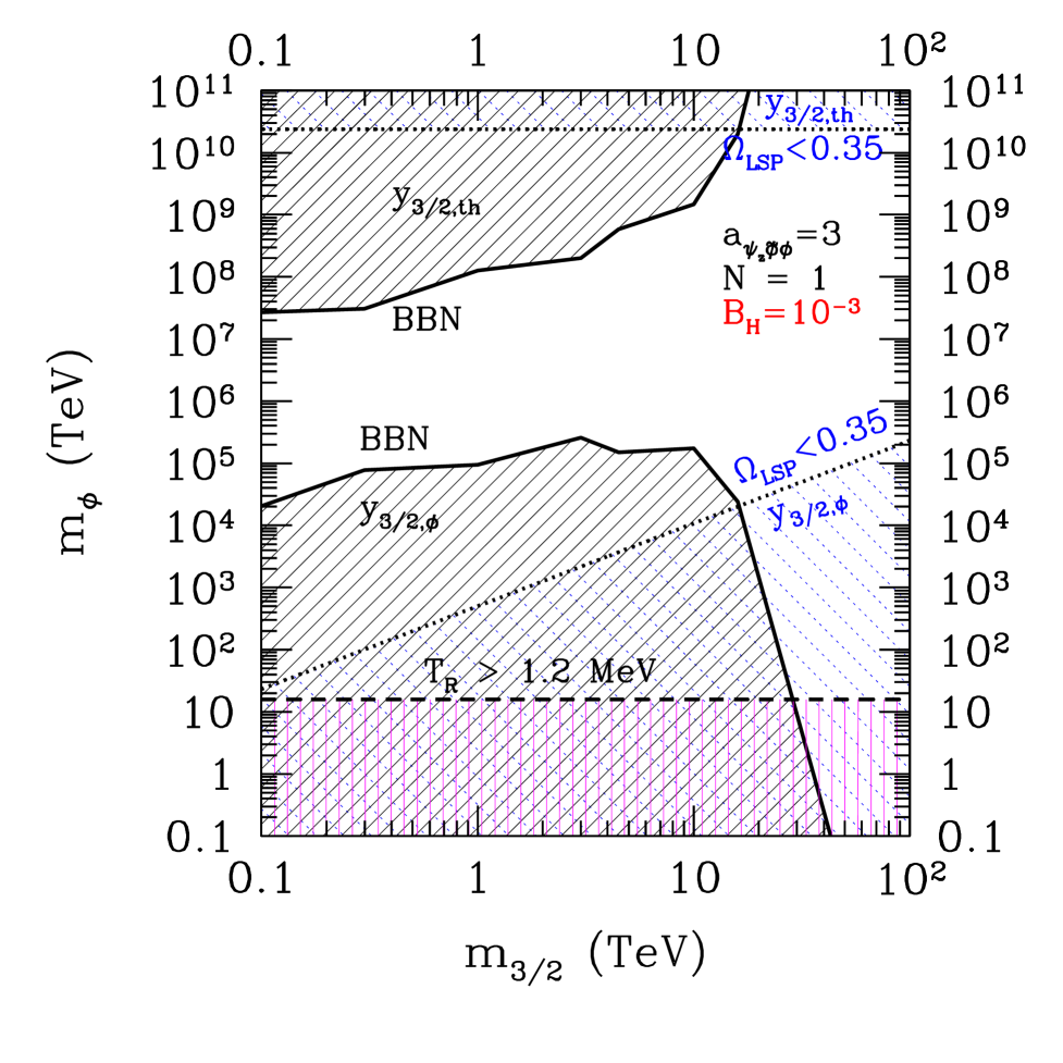
In Fig. 1, we plot the resultant constraints on as a function of for the case and the hadronic branching ratio . Here we have taken and in Eq. (16). We find that the reheating requirement (23) gives a milder lower bound on . From Fig. 1, we see that the modulus mass of the weak scale is excluded for gravitino mass of = 0.1 – 100 . In addition, it is interesting that we can obtain the upper bound on by this type of cosmological arguments. Finally we comment on the dependence of our constraints in Fig. 1 on . Since appears only in the form in all of the relevant expressions in Eqs. (21), (26) and (28), the constraints for other than can easily be read off by replacing in the vertical axis by in Fig. 1.
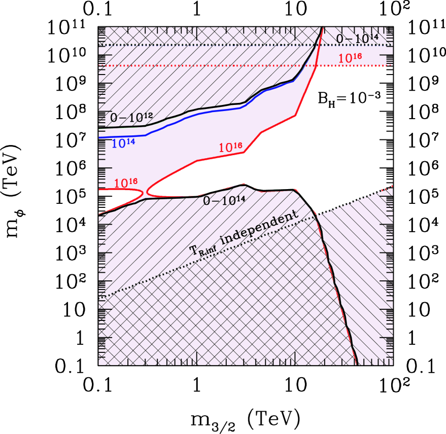
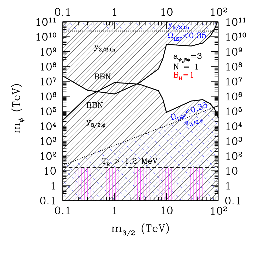
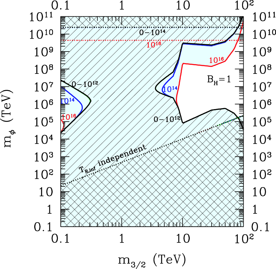
Next we discuss the more general situation where can also be important with . We plot the constraints on as a function of in Fig. 2 in the case . The extent of oblique lines coincides exactly with those excluded from the constraints by BBN and LSP in Fig. 1, which correspond to the limiting cases that is sufficiently low such as GeV, namely, . For higher reheating temperatures e.g., = 1014 – 1016 GeV, larger parameter regions are additionally excluded. The shadowed region corresponds to the excluded region for GeV with or for . In a similar fashion, the constraints for the case are depicted in Fig. 3 and Fig. 4 for and , respectively. From these figures, we see that larger regions are excluded for .
It is important to note that although the excluded region becomes broader for higher reheating temperature, we still have a fairly large allowed region in our parameter space even for the highest possible reheating temperature GeV thanks to the dilution of primordial gravitinos by the entropy production associated with modulus decay. Thus the previous upper bound on in (43) can easily be relaxed if we consider the decaying moduli. In Table 1 (Table 2) we show the allowed values of for various and for the case ().
V Conclusion
We have studied the effects of decaying modulus oscillation on the cosmological gravitino problem. We have considered a new direct production mechanism of gravitinos from modulus decay, namely, a decay mode of modulus into a gravitino and a modulino. The width of this decay mode can be larger than the other mode into two gravitinos which has been studied in [38], if the coupling constant is of the same order of magnitude with .
Comparing our yield of gravitinos with the constraints imposed by BBN and the relic LSPs, which are decay products of gravitinos, we have obtained a constraint on the masses of gravitinos and modulus. As a result we have found that due to the above-mentioned direct production of gravitinos from decaying modulus, the modulus mass with TeV is excluded, even when the branching ratio into hadrons is minimal.
On the other hand, we have also found that wide range of and are still allowed even if the reheating temperature after inflation is as high as GeV and the effects on the hadronic decay of the gravitinos are taken into account, thanks to the dilution of primordial gravitinos due to the entropy production associated with modulus decay.
Thus in order to study cosmological consequences of gravitinos, it is important to analyze not only their abundance right after inflation but also their subsequent dilution due to late-time entropy production, as well as late-time production from scalar condensates with only gravitationally suppressed interactions including a dilaton and a Polonyi field.
Acknowledgments
This work was partially supported by the JSPS Grants-in Aid of the Ministry of Education, Science, Sports, and Culture of Japan No. 15-03605 (KK), No. 13640285 (JY), and No.12047201 (MY).
REFERENCES
- [1] S. Weinberg, Phys. Rev. Lett. 48, 1303 (1982).
- [2] L. M. Krauss, Nucl. Phys. B 227, 556 (1983).
- [3] D. Lindley, Astrophys. J. 294 (1985) 1.
- [4] M. Y. Khlopov and A. D. Linde, Phys. Lett. B 138, 265 (1984); F.Balestra, G.Piragino, D.B.Pontecorvo, M.G.Sapozhnikov, I.V.Falomkin, M.Yu.Khlopov, Sov. J. Nucl. Phys. 39 (1984) 626; M.Yu. Khlopov, Yu.L.Levitan, E.V.Sedelnikov and I.M.Sobol, Phys. Atom.Nucl. 57 (1994) 1393; M. Y. Khlopov, “Cosmoparticle Physics,” (Singapore: World Scientific, 1999)
- [5] J. R. Ellis, J. E. Kim and D. V. Nanopoulos, Phys. Lett. B 145, 181 (1984).
- [6] R. Juszkiewicz, J. Silk and A. Stebbins, Phys. Lett. B 158, 463 (1985).
- [7] J. R. Ellis, D. V. Nanopoulos and S. Sarkar, Nucl. Phys. B 259 (1985) 175.
- [8] J. Audouze, D. Lindley and J. Silk, Astrophys. J. 293, L53 (1985) ; D. Lindley, Phys. Lett. B 171 (1986) 235.
- [9] M. Kawasaki and K. Sato, Phys. Lett. B 189, 23 (1987).
- [10] R. J. Scherrer and M. S. Turner, Astrophys. J. 331 (1988) 19.
- [11] R. Dominguez-Tenreiro, Astrophys. J. 313, 523 (1987).
- [12] M. H. Reno and D. Seckel, Phys. Rev. D 37 (1988) 3441.
- [13] S. Dimopoulos, R. Esmailzadeh, L. J. Hall and G. D. Starkman, Astrophys. J. 330, 545 (1988) ; Phys. Rev. Lett. 60, (1988) 7 ; Nucl. Phys. B 311 (1989) 699.
- [14] J. R. Ellis, G. B. Gelmini, J. L. Lopez, D. V. Nanopoulos and S. Sarkar, Nucl. Phys. B 373, 399 (1992).
- [15] M. Kawasaki and T. Moroi, Prog. Theor. Phys. 93 (1995) 879 [arXiv:hep-ph/9403364] ; Astrophys. J. 452, 506 (1995) [arXiv:astro-ph/9412055].
- [16] M. Kawasaki and T. Moroi, Phys. Lett. B 346, 27 (1995) [arXiv:hep-ph/9408321].
- [17] R. J. Protheroe, T. Stanev and V. S. Berezinsky, Phys. Rev. D 51, 4134 (1995) [arXiv:astro-ph/9409004].
- [18] E. Holtmann, M. Kawasaki, K. Kohri and T. Moroi, Phys. Rev. D 60, 023506 (1999) [arXiv:hep-ph/9805405].
- [19] K. Jedamzik, Phys. Rev. Lett. 84, 3248 (2000) [arXiv:astro-ph/9909445].
- [20] M. Kawasaki, K. Kohri and T. Moroi, Phys. Rev. D 63, 103502 (2001) [arXiv:hep-ph/0012279].
- [21] K. Kohri, Phys. Rev. D 64 (2001) 043515 [arXiv:astro-ph/0103411].
- [22] R. H. Cyburt, J. R. Ellis, B. D. Fields and K. A. Olive, Phys. Rev. D 67, 103521 (2003) [arXiv:astro-ph/0211258].
- [23] M. Kawasaki, K. Kohri and T. Moroi, arXiv:astro-ph/0402490.
- [24] H. Pagels and J. R. Primack, Phys. Rev. Lett. 48, 223 (1982).
- [25] V. S. Berezinsky, Phys. Lett. B 261, 71 (1991).
- [26] T. Moroi, H. Murayama and M. Yamaguchi, Phys. Lett. B 303, 289 (1993).
- [27] T. Moroi, arXiv:hep-ph/9503210.
- [28] M. Bolz, A. Brandenburg and W. Buchmuller, Nucl. Phys. B 606, 518 (2001) [arXiv:hep-ph/0012052].
- [29] A. D. Linde, Phys. Lett. B 259, 38 (1991); Phys. Rev. D 49, 748 (1994).
- [30] M. Kawasaki, M. Yamaguchi, and J. Yokoyama, Phys. Rev. D 68, 023508 (2003); M. Yamaguchi and J. Yokoyama, Phys. Rev. D 68, 123530 (2003); M. Yamaguchi and J. Yokoyama, hep-ph/0402282.
- [31] G. D. Coughlan, W. Fischler, E. W. Kolb, S. Raby and G. G. Ross, Phys. Lett. B 131, 59 (1983).
- [32] T. Banks, D. B. Kaplan and A. E. Nelson, Phys. Rev. D 49, 779 (1994) [arXiv:hep-ph/9308292].
- [33] B. de Carlos, J. A. Casas, F. Quevedo and E. Roulet, Phys. Lett. B 318, 447 (1993) [arXiv:hep-ph/9308325].
- [34] T. Moroi, M. Yamaguchi and T. Yanagida, Phys. Lett. B 342, 105 (1995) [arXiv:hep-ph/9409367].
- [35] M. Kawasaki, T. Moroi and T. Yanagida, Phys. Lett. B 370, 52 (1996) [arXiv:hep-ph/9509399].
- [36] T. Moroi and L. Randall, Nucl. Phys. B 570, 455 (2000) [arXiv:hep-ph/9906527].
- [37] M. Kawasaki, K. Kohri and N. Sugiyama, Phys. Rev. Lett. 82, 4168 (1999) [arXiv:astro-ph/9811437]; Phys. Rev. D 62, 023506 (2000) [arXiv:astro-ph/0002127].
- [38] M. Hashimoto, K. I. Izawa, M. Yamaguchi and T. Yanagida, Prog. Theor. Phys. 100, 395 (1998) [arXiv:hep-ph/9804411].
- [39] S. B. Giddings, S. Kachru and J. Polchinski, Phys. Rev. D 66, 106006 (2002) [arXiv:hep-th/0105097].
- [40] V. S. Kaplunovsky and J. Louis, Phys. Lett. B 306, 269 (1993) [arXiv:hep-th/9303040].
- [41] D. H. Lyth and E. D. Stewart, Phys. Rev. D 53, 1784 (1996) [arXiv:hep-ph/9510204].
- [42] D. N. Spergel et al., Astrophys. J. Suppl. 148, 175 (2003) [arXiv:astro-ph/0302209].
- [43] W. Freedman et al., Astrophys. J. 553, 47 (2001).
- [44] J.C. Mather et al., Astrophys. J. 512, 511 (1999).
| = 0- GeV | GeV | ||||
|---|---|---|---|---|---|
| 0.1 TeV | TeV | TeV | TeV | ||
| 0.3 TeV | TeV | TeV | excluded | ||
| 1 TeV | TeV | TeV | TeV | ||
| 3 TeV | TeV | TeV | TeV | ||
| 10 TeV | TeV | TeV | TeV | ||
| 30 TeV | TeV | TeV | TeV | ||
| 100 TeV | TeV | TeV | TeV |
| = 0- GeV | GeV | ||||
|---|---|---|---|---|---|
| 0.1 TeV | TeV | TeV | TeV | ||
| 0.3 TeV | TeV | excluded | excluded | ||
| 1 TeV | excluded | excluded | excluded | ||
| 3 TeV | excluded | excluded | excluded | ||
| 10 TeV | TeV | TeV | TeV | ||
| 30 TeV | TeV | TeV | TeV | ||
| 100 TeV | TeV | TeV | TeV |