Hyperon polarization in different inclusive production processes in unpolarized high energy hadron-hadron collisions

Abstract

We apply the picture proposed in a previous Letter, which relates the hyperon polarization in unpolarized hadron-hadron collisions to the left-right asymmetry in singly polarized reactions, to the production of different hyperons in reactions using different projectiles and/or targets. We discuss the different ingredients of the proposed picture in detail and present the results for hyperon polarization in the reactions such as $pp$, $K^{-}p$, $\pi^{\pm}p$, and $\Sigma^{-}p$ collisions. We compare the results with the available data and make predictions for future experiments.

I introduction

Since the discovery Les75 ; Bun76 in 1970s, the surprisingly large transverse polarization of hyperons in unpolarized high energy hadron-hadron and hadron-nucleus collisions has been a standing hot topic in High Energy Spin Physics (see e.g, Les75 ; Bun76 ; Hel96 ; And79 ; Deg81 ; Szw81 ; Pon85 ; Bar92 ; Sof92 ; LB97 ; LB00 ; LLts00 ; Ans01 , and the references cited therein.). Experimentally, there are a large number of similar experiments that have been performed at different energies and/or using different projectiles and/or targets and for the production of different hyperons Hel96 . Theoretically, different models have been proposed And79 ; Deg81 ; Szw81 ; Pon85 ; Bar92 ; Sof92 ; LB97 ; LB00 ; LLts00 ; Ans01 , the aim of which is to understand the origin(s) of this striking spin effect in high energy reactions. Clearly such studies should provide us with useful information on the spin structure of the hadron and the spin dependence of strong interactions.

Inspired by the similarities of the corresponding data Hel96 ; ANdata ; E704 , we proposed a new approach in a recent Letter LB97 to understand the origin(s) of the transverse hyperon polarization in unpolarized hadron-hadron collisions by relating them to the left-right asymmetries observed ANdata ; E704 in singly polarized $pp$ collisions. We pointed out that these two striking spin phenomena should be closely related to each other and have the same origin(s). We showed that using the spin correlation deduced from the single-spin left-right asymmetries for inclusive $\pi$ production as input, we can naturally understand the transverse polarization for a hyperon which has one valence quark in common with the projectile, such as $\Sigma^{-}$, $\Xi^{0}$, or $\Xi^{-}$ in $pp$ collisions, or $\Lambda$ in $K^{-}p$ collisions. We showed also that, to understand the puzzling transverse polarization of $\Lambda$ in $pp$ collisions, which have two valence quarks in common with the projectile, we need to assume that the $s$ and $\bar{s}$, which combine respectively with the valence-($ud$) diquark and the remaining $u$-valence quark to form the produced $\Lambda$ and the associatively produced $K^{+}$ in the fragmentation region, should have opposite spins. Under this assumption, we obtained a good quantitative fit to the $x_{F}$ dependence of $\Lambda$ polarization in $pp$ collisions (where $x_{F}\equiv 2p_{\|}/\sqrt{s}$, $p_{\|}$ is the longitudinal component of the momentum of the produced hyperon, and $\sqrt{s}$ is the total center of mass energy of the $pp$ system). The obtained qualitative features for the polarizations of other hyperons are all in good agreement with the available data.

There are two main points in the picture that need to be further tested, i.e., (i) the $s$ and $\bar{s}$ that combine respectively with the valence-($ud$) diquark and the remaining $u$-valence quark of the projectile proton to form the produced $\Lambda$ and the associatively produced $K^{+}$ in the fragmentation region have opposite spins, and (ii) the SU(6) wave function can be used to describe the relation between the spin of the fragmenting quark and that of the hadron produced in the fragmentation process. Developments have been made since the publication of Ref. LB97 . We found out that exclusive reactions such as $pp\to p\Lambda K^{+}$ and $e^{-}p\to e^{-}\Lambda K^{+}$ are best suitable to test point (i). We therefore applied the picture to these processes and presented the obtained results in Refs. LB00 and LX02 . It is encouraging to see that these results are all in agreement with the available data R608 ; CLAS03 .

It has also been pointed out BL98 that the longitudinal polarization of $\Lambda$ in $e^{+}e^{-}$ annihilation at $Z^{0}$ pole provides a special test to point (ii), i.e., whether SU(6) wave function can be used in relating the spin of the fragmenting quark to that of the produced hadron. Calculations have been made BL98 ; GH93 and the obtained results are consistent with the data Aleph96 ; OPAL98 . Since neither the accuracy nor the abundance of the data is high enough to give a conclusive judgment, we made a systematic study BL98 ; LL00 of hyperon polarization in other reactions which can be used to test this point. The results are in agreement with the available data Aleph96 ; OPAL98 ; NOMAD00 and future experiments are under way.

Encouraged by these developments, in this paper, we apply the proposed picture to study the polarizations of different hyperons in different unpolarized hadron-hadron and hadron-nucleus reactions. We summarize the different ingredients of the picture and their developments in detail in Sec. II. In Sec. III, we give the calculation method of hyperon polarization in different processes using the picture. In Sec. IV, we apply the method to calculate the polarizations of different hyperons produced in unpolarized $pp$, $K^{-}p$, $\pi^{\pm}p$, and $\Sigma^{-}p$ collisions. We present the results obtained and compare them with the available data. Finally, a short summary and outlook is given in Sec. V.

II the physical picture

In this section, we summarize the key points of the picture proposed in Ref. LB97 . The basic idea of the picture is that there should be a close relation between hyperon polarization ($P_{H}$) in unpolarized hadron-hadron collisions and the left-right asymmetry ($A_{N}$) in single-spin hadron-hadron collisions. Hence, if we extract the essential information encoded in the $A_{N}$ data, we can study $P_{H}$ based on such information. There are three key points in this physical picture which are summarized as the following.

II.1 Correlation between the spin of the quark and the direction of motion of the produced hadron

It has been pointed out LB97 that the existence of $A_{N}$ in singly polarized hadron-hadron collision implies the existence of a spin correlation between the spin of the fragmenting quark and the direction of momentum of the produced hadron, i.e., $\vec{s}_{q}\cdot\vec{n}$ type of spin correlation in the reaction. [Here, $\vec{s}_{q}$ is the spin of the quark; $\vec{n}\equiv(\vec{p}_{inc}\times\vec{p}_{h})/|\vec{p}_{inc}\times\vec{p}_{h}|$ is the unit vector in the normal direction of the production plane, $\vec{p}_{inc}$ and $\vec{p}_{h}$ are respectively the momentum of the incident hadron and that of the produced hadron.] One of the major ingredients of the picture proposed in Ref. LB97 is that both the existence of $A_{N}$ and that of $P_{H}$ are different manifestations of this spin correlation $\vec{s}_{q}\cdot\vec{n}$. Hence we can use the experimental results for $A_{N}$ as input to determine the strength of this spin correlation, then apply it to unpolarized hadron-hadron collision to study $P_{H}$.

We recall that ANdata ; E704 ; LB00rev , in the language commonly used in describing $A_{N}$, the polarization direction of the incident proton is called upward, and the incident direction is forward. The single-spin left-right asymmetry $A_{N}$ is just the difference between the cross section where $\vec{p}_{h}$ points to the left and that to the right, which corresponds to $\vec{s}_{q}\cdot\vec{n}=1/2$ and $\vec{s}_{q}\cdot\vec{n}=-1/2$, respectively. The data ANdata ; E704 on $A_{N}$ show that if a hadron is produced by an upward polarized valence quark of the projectile, it has a large probability to have a transverse momentum pointing to the left. $A_{N}$ measures the excess of hadrons produced to the left over those produced to the right. The difference of the probability for the hadron to go left and that to go right is denoted BLM93 ; LB00rev by $C$ if the hadron is produced by an upward polarized quark. $C$ is a constant in the range of $0<C<1$. It has been shown that BLM93 ; LB00rev , to fit the $A_{N}$ data E704 in the transverse momentum interval $0.7<p_{T}<2.0$ GeV/$c$, $C$ should be taken as $C=0.6$.

In terms of the spin correlation discussed above, the cross section should be expressed as

$$\sigma=\sigma_{0}+(\vec{s}_{q}\cdot\vec{n})\sigma_{1},$$ (1)

where $\sigma_{0}$ and $\sigma_{1}$ are independent of $\vec{s}_{q}$. The second term just denotes the existence of the $\vec{s}_{q}\cdot\vec{n}$ type of spin correlation. $C$ is just the difference between the cross section where $\vec{s}_{q}\cdot\vec{n}=1/2$ and that where $\vec{s}_{q}\cdot\vec{n}=-1/2$ divided by the sum of them, i.e., $C=\sigma_{1}/(2\sigma_{0})$.

Now, we assume the same strength for the spin correlation in hyperon production in the same collisions. It follows that the quark which fragments into the hyperon should be polarized, and the polarization $P_{q}$ can be determined by using Eq. (1). Since both the left-right asymmetry in singly polarized collision and hyperon polarization in unpolarized collision exist mainly in large $x_{F}$ region, we assume that the spin correlation exists only for valence quarks of the incident hadrons. For a hyperon produced with momentum $\vec{p}_{h}$, $\vec{n}$ is given. The cross section that this hyperon is produced in the fragmentation of a valence quark with spin satisfying $\vec{s}_{q}\cdot\vec{n}=1/2$ is $(\sigma_{0}+\sigma_{1}/2)$, and that with spin satisfying $\vec{s}_{q}\cdot\vec{n}=-1/2$ is $(\sigma_{0}-\sigma_{1}/2)$. Hence, the polarization of the valence quarks which lead to the production of the hyperons with that $\vec{n}$ is given by,

$$P_{q}=\frac{(\sigma_{0}+\sigma_{1}/2)-(\sigma_{0}-\sigma_{1}/2)}{(\sigma_{0}+\sigma_{1}/2)+(\sigma_{0}-\sigma_{1}/2)}=\frac{\sigma_{1}}{2\sigma_{0}}=C.$$ (2)

It should be emphasized that $P_{q}\neq 0$ just means that the strength of the spin correlation of the form $\vec{s}_{q}\cdot\vec{n}$ is nonzero in the reaction. It means that, due to some spin-dependent interactions, the quarks which have spins along the same direction as the normal of the production plane have a large probability to combine with suitable sea quarks to form the specified hyperons than those which have spins in the opposite direction. It does not imply that the quarks in the unpolarized incident hadrons were polarized in a given direction, which would contradict the general requirement of space rotation invariance. In fact, in an unpolarized reaction, the normal of the production plane of the specified hyperons is uniformly distributed in the transverse directions. Hence, averaging over all the normal directions, the quarks are unpolarized.

We would like also to mention that similar idea has been applied XL03 to spin alignments of vector mesons in unpolarized hadron-hadron collisions. It has been shown that the existence of the spin alignment of vector mesons in unpolarized hadron-hadron collision is another manifestation of the existence of the $\vec{s}_{q}\cdot\vec{n}$ type of spin correlation. The obtained result are in agreement with the available data Chl72 ; Bar83 ; EXCHARM00 .

II.2 Relating the spin of the quark to that of the hadron

As discussed in the above-mentioned subsection, the existence of the $\vec{s}_{q}\cdot\vec{n}$ type of spin correlation in hadron-hadron collision implies a polarization of the quark $q^{0}$ transverse to the production plane of the hyperon. (Here, we use the superscript $0$ to denote the quark before fragmentation.) To study the polarization of the produced hyperon from this point, we need to know the relation between the spin of the quark and that of the hadron produced in the fragmentation of this quark. The question of the relation between the spin of the fragmenting quark $q^{0}$ and that of the hadron created in the fragmentation of $q^{0}$ is usually referred to as “spin transfer in high energy fragmentation process”. It contains two parts: will $q^{0}$ keep its polarization in the fragmentation? what is the relation between the spin of $q^{0}$ and that of the hadron which contains $q^{0}$?

The answers to these questions depend on the spin structure of hadron and the hadronization mechanism. They can even be different in the longitudinally polarized case from those for the transversely polarized case. Since neither of them can be solved using perturbative calculations, presently, phenomenological studies are need to search the answers to them. Currently, there exist two distinct pictures for the spin structure of nucleon, i.e., the SU(6) picture based on the SU(6) wave function of the baryon, and the DIS picture based on the polarized deeply inelastic lepton-nucleon scattering data and other inputs such as symmetry assumptions and data from other experiments. It is of particular interest to know which one is suitable here.

It is clear that to study these questions, one needs to know the polarization of the quark before fragmentation and measure the polarization of the hadron produced in the fragmentation. Hence, we have the following two possibilities: One is to study hyperon polarization in $e^{+}e^{-}$ annihilation at $Z^{0}$ pole, in polarized $ep$ deeply inelastic scattering or in high $p_{T}$ polarized $pp$ collision. The other is to study the vector meson polarization in these processes.

It has been pointed out that the $\Lambda$ polarization in $e^{+}e^{-}$ annihilation at the $Z^{0}$ pole provides a very special test to the applicability of the SU(6) picture in the longitudinally polarized case. This is because, for $e^{+}e^{-}\to Z^{0}\to\Lambda X$, the $s\bar{s}$ created at the $e^{+}e^{-}$ annihilation vertex is almost completely longitudinally polarized. In this case, if we assume that the quark keeps its polarization in the fragmentation and use the SU(6) wave function to connect the spin of the quark and that of the hyperon that contains this quark, we should obtain a maximum for the magnitude of $\Lambda$ polarization since in this picture the spin of the $s$-quark is completely transferred to $\Lambda$. Experimental data were obtained Aleph96 ; OPAL98 for $e^{+}e^{-}\to Z^{0}\to\Lambda X$ by the ALEPH and OPAL Collaborations at LEP. We showed BL98 that if we assume that the $q^{0}$ keeps its polarization in fragmentation and the SU(6) wave function can be used in relating the polarization of $q^{0}$ and that of the produced hyperon which contains $q^{0}$, we obtain the results which are in agreement with the data. This result is rather encouraging. But, the accuracy and abundance of the data are not enough to make a conclusive judgment. In particular, there is no direct measurement available at all in the transversely polarized case. We therefore made a systematic calculation for hyperon polarizations in all the different reactions LL00 . There are also data for $\Lambda$ polarization in deeply inelastic scattering NOMAD00 , they are also consistent with the results obtained using the SU(6) picture.

There are also data that provide information on vector meson polarization in high energy reactions. The $00$-elements of the helicity density matrices for $K^{*}$, $\rho$, etc in $e^{+}e^{-}\to Z^{0}\to VX$ have been measured ALEPH95 ; DELPHI95 ; OPAL97 by the ALEPH, DELPHI and OPAL Collaborations at LEP. We showed XLL01 that these data can also be understood using the SU(6) picture. Further tests, not only in the longitudinally polarized case but also in the transversely polarized case, are under way. In this paper, we assume it is the same in longitudinally and transversely polarized cases and use it in studying hyperon polarization in unpolarized high energy hadron-hadron collisions.

Having the two points discussed in the last and this subsections, we can already obtain the polarizations for those hyperons which have one valence quark of the same flavor as that of the projectile, e.g., $pp\to\Sigma^{-}X$, $K^{-}p\to\Lambda X$ and $\Sigma^{-}p\to\Sigma^{+}X$. Some of the qualitative features of the results are given in Ref. LB97 . It is encouraging to see that all of them are in good agreement with the data Hel96 .

II.3 Correlation between the spin of $q_{s}$ and that of $\bar{q}_{s}$ which combine with the $(q_{v}q_{v})$ and remaining $q_{v}$ to form the produced hyperon and the associated meson

To study the polarization of hyperons such as $\Lambda$ in $pp\to\Lambda X$, i.e., those which have two valence quarks that have the same flavors as those of the projectile, we encounter the following question: If a hadron is produced by two valence quarks (valence diquark) $q_{v}q_{v}$ of the projectile, the remaining valence quark $q_{v}$ produces an associated hadron. What are the spin states of the $q_{s}$ and $\bar{q}_{s}$ that combine with the $q_{v}q_{v}$ and the remaining $q_{v}$ to form the produced hyperon and the associatively produced meson in the fragmentation region, respectively?

Theoretically, it is quite difficult to derive it since we are in the very small $x$ region; the production of such pairs is also of soft nature in general and cannot be calculated using perturbative theory. To get some clue to this problem, we still start from the single-spin left-right asymmetry $A_{N}$. The existing data ANdata ; E704 clearly show that $A_{N}$ in $p^{\uparrow}p\to\Lambda X$ is large in magnitude and negative in sign in the fragmentation region. We note that the $\Lambda$ in this region is mainly produced by the valence-$(u_{v}d_{v})$-diquark of the projectile and is associated with the production of a $K^{+}$ produced by the remaining $u_{v}$. From the SU(6) wave function we learn that the $(u_{v}d_{v})$ has to be in the spin zero state and the spin of the proton is carried by the remaining $u_{v}$. According to the $\vec{s}_{q}\cdot\vec{n}$ spin correlation discussed in Subsection II.1, $A_{N}$ for the associatively produced $K^{+}$ is positive. Hence, to understand the data on $A_{N}$ for $\Lambda$, we simply need to assume BL96 that $\Lambda$ produced by $(u_{v}d_{v})$ and $K^{+}$ that is associatively produced by the remaining $u_{v}$ move in the opposite transverse directions, which is just a direct consequence of transverse momentum conservation. Now, we apply this to unpolarized $pp$ collision and consider the case that a $\Lambda$ is produced by $(u_{v}d_{v})$ together with a $s$-quark and a $K^{+}$ is associatively produced by the remaining $u_{v}$ together with the $\bar{s}$. According to the $\vec{s}_{q}\cdot\vec{n}$ spin correlation mentioned in Subsection II.1, the remaining $u_{v}$ should have a large probability to be polarized in $-\vec{n}$ direction since the normal of the production plane for the $K^{+}$ is opposite to the normal $\vec{n}$ of the production plane of $\Lambda$. The polarization is $-C$. Since $K^{+}$ is a spin zero object, the $\bar{s}$ should have a polarization of $+C$ (in the $\vec{n}$ direction). The data for $\Lambda$ polarization show that $P_{\Lambda}$ is large and negative. This means that the $s$-quark has a negative polarization. We thus reach the conclusion that, to understand the polarization of $\Lambda$ in $pp\to\Lambda X$, we need to assume that the $s$ and $\bar{s}$ have opposite spins. Under this assumption, together with the two points mentioned in the last two subsections, we obtained LB97 a good fit to the data on $\Lambda$ polarization.

This point needs of course to be further studied and tested experimentally. We found out that the simple exclusive process are most suitable for this purpose. Hyperon polarizations in the exclusive processes such as $pp\to p\Lambda K^{+}$ and $e^{-}p\to e^{-}\Lambda K^{+}$ are very sensitive to the spin states of the $s$ and $\bar{s}$ pairs. If the $s$ and $\bar{s}$ have opposite spins, the obtained results for $\Lambda$ polarization in $pp\to p\Lambda K^{+}$ should take the maximum among the different channels for $pp\to\Lambda X$. This is because that here we have a situation that the $\Lambda$ is definitely produced by the $(u_{v}d_{v})$ valence diquark and is definitely associated with a $K^{+}$ that is definitely produced by the remaining $u_{v}$ of the incident $p$. Hence, we obtain that in this case, $P_{\Lambda}=-C=-0.6$. This is in good agreement with the data obtained R608 by the R608 Collaboration at CERN which show that $P_{\Lambda}=-0.62\pm 0.04$.

We also calculated LX02 $\Lambda$ polarization in $e^{-}p\to e^{-}\Lambda K^{+}$ in all three cases in which the spin states of $s$ and $\bar{s}$ can be, i.e., opposite, same or uncorrelated. We found out that the results in the three cases are quite different from each other. Now, experimental data are obtained CLAS03 for $\Lambda$ polarization in $e^{-}p\to e^{-}\Lambda K^{+}$ by the CLAS Collaboration at Jefferson Laboratory. Comparing to the data, we see that the results obtained in the case that the spins of $s$ and $\bar{s}$ are opposite are favored. Further tests are also under way.

We now assume that this is in general true, i.e., the $q_{s}$ that combines with the $(q_{v}q_{v})$ of the projectile to form the hyperon and the $\bar{q}_{s}$ that combines with the remaining $q_{v}$ to form the associatively produced meson have opposite spins. Under this assumption, we obtain the result that the $q_{s}$ should be polarized in the $-\vec{n}$ direction and the polarization is $-C$. We apply this to the production of different hyperons to calculate the hyperon polarizations in unpolarized high energy hadron-hadron or hadron-nucleus collisions in next sections.

We emphasize that the above mentioned result is true for the production of hyperons associated with the production of pseudo-scalar mesons. The situation should be different if the associatively produced meson is a vector meson. This influence will be further investigated in a separate paper DLfuture and here we consider only the former case.

III the calculation method

Having the picture discussed in last section, we can calculate the hyperon polarization in different hadron-hadron collisions. We now present the formulas used in these calculations.

III.1 General formulas

We consider the process $P+T\to H_{i}+X$, where $P$ and $T$ denote respectively the projectile and target hadron, and $H_{i}$ denotes the $i$th kind of the hyperons. The hyperon polarization $P_{H_{i}}$ is defined as,

$$P_{H_{i}}(x_{F}|s)\equiv\frac{N(x_{F},H_{i},\uparrow|s)-N(x_{F},H_{i},\downarrow|s)}{N(x_{F},H_{i},\uparrow|s)+N(x_{F},H_{i},\downarrow|s)}=\frac{\Delta N(x_{F},H_{i}|s)}{N(x_{F},H_{i}|s)},$$ (3)

where $N(x_{F},H_{i},l|s)$ is the number density of $H_{i}$’s polarized in the same ($l=\uparrow$) or opposite ($l=\downarrow$) direction as the normal ($\vec{n}$) of the production plane at a given $\sqrt{s}$; $x_{F}\equiv 2p_{\|}/\sqrt{s}$, $p_{\|}$ is the longitudinal momentum of $H_{i}$ with respect to the incident direction of $P$, and $\sqrt{s}$ is the total c.m. energy of the colliding hadron system. It is clear that the denominator is nothing else but the number density of $H_{i}$ without specifying the polarization.

To calculate $\Delta N(x_{F},H_{i}|s)$, we divide the final hyperons $H_{i}$’s into the following four groups according to the different origins for the production: (A) those directly produced and contain a valence diquark (two valence quarks) $(q_{v}q_{v})^{P}$ of the projectile; (B) those directly produced and contain a valence quark $q_{v}^{P}$ of the projectile; (C) those from the decay of the directly produced heavier hyperons $H_{j}$’s that contain a $(q_{v}q_{v})^{P}$ or a $q_{v}^{P}$; and (D) the others. In this way, we have,

$$N(x_{F},H_{i}|s)=N_{0}(x_{F},H_{i}|s)+D^{A}(x_{F},H_{i}|s)+\sum_{f}{D^{B,f}(x_{F},H_{i}|s)}+\sum_{j}{D^{C,H_{j}}(x_{F},H_{i}|s)},$$ (4)

where $D^{A}(x_{F},H_{i}|s)$, $D^{B,f}(x_{F},H_{i}|s)$ and $D^{C,H_{j}}(x_{F},H_{i}|s)$ denote the contributions from groups (A), (B) and (C), respectively; the superscript $f$ and $j$ denote the flavor of $q_{v}$ and the type of $H_{j}$, respectively; $N_{0}$ is the contribution from (D).

According to the picture discussed in last section, hyperons from groups (A), (B) and (C) can be polarized, while those from (D) are not. This means that those from (A), (B) and (C) contribute to the numerator $\Delta N$ of Eq. (4), i.e., we have,

$$\Delta N(x_{F},H_{i}|s)=\Delta D^{A}(x_{F},H_{i}|s)+\sum_{f}{\Delta D^{B,f}(x_{F},H_{i}|s)}+\sum_{j}{\Delta D^{C,H_{j}}(x_{F},H_{i}|s)}.$$ (5)

Since valence quarks usually carry large fractions of the momenta of the incident hadrons, we expect that, for very large $x_{F}$, $D^{A}(x_{F},H_{i}|s)$ dominates. For small $x_{F}$, $N_{0}$ dominates, while for moderate $x_{F}$, $D^{B}(x_{F},H_{i}|s)$ plays the dominant role. Hence, if we neglect the decay contributions, we expect from Eqs. (3–5) that $P_{H_{i}}(x_{F}|s)$ has the following general properties. For $x_{F}$ increasing from 0 to 1, it starts from 0, increases to ${\sum_{f}{\Delta D^{B,f}(x_{F},H_{i}|s)}}/{\sum_{f}{D^{B,f}(x_{F},H_{i}|s)}}$, and finally tends to ${\Delta D^{A}(x_{F},H_{i}|s)}/{D^{A}(x_{F},H_{i}|s)}$ at $x_{F}\to 1$. We will come to this point in next section for particular hyperon in the specified reaction. We now first discuss the calculations of all these $D$’s, $\Delta D$’s and $N_{0}$ in the following.

III.2 Calculations of $D$’s and $N_{0}$

The contributions of hyperons from the different groups discussed above are entirely determined by the hadronization mechanisms in unpolarized case. They are independent of the polarization of the hadrons. We can calculate them using a hadronization model that gives a good description of the unpolarized data. For this purpose, the simple model used in Refs. BLM93 ; BL96 ; LB00rev is a very practical choice. In this model, hyperons from groups (A) and (B) are described as the products of the following “direct-formation” or “direct-fusion” process. For (A), it is,

$$(q_{v}q_{v})^{P}+q_{s}^{T}\to H_{i},$$

and for (B), it is,

$$q_{v}^{P}+(q_{s}q_{s})^{T}\to H_{i},$$

where $q_{s}^{T}$ and $(q_{s}q_{s})^{T}$ denote a sea quark or a sea diquark from the target. The number densities of the hyperons produced in these processes are determined by the number densities of the initial partons. They are given by BLM93 ; BL96 ; LB00rev ,

$$D^{A}(x_{F},H_{i}|s) = \kappa_{H_{i}}^{d}f^{P}_{D}(x^{P}|q_{v}q_{v})q^{T}_{s}(x^{T}),$$ (6)

$$D^{B,f}(x_{F},H_{i}|s) = \kappa_{H_{i}}q^{P}_{v}(x^{P})f^{T}_{D}(x^{T}|q_{s}q_{s}),$$ (7)

where, $x^{P}\approx x_{F}$ and $x^{T}\approx m_{H_{i}}^{2}/(sx_{F})$, followed from energy-momentum conservation in the direct formation processes; $q_{i}(x)$ is the quark distribution function, where $q$ denotes the flavor of the quark and the subscript $i=v$ or $s$ denotes whether it is for valence or sea quarks; $f_{D}(x|q_{i}q_{j})$ is the diquark distribution functions, where $q_{i}q_{j}$ denotes the flavor and whether they are valence or sea quarks, the superscripts $P$ or $T$ denote the name of the hadron; $\kappa_{H_{i}}^{d}$ and $\kappa_{H_{i}}$ are two constants which are fixed by fitting two data points in the large $x_{F}$ region.

Since most of the decay process $H_{j}\to H_{i}+X$ that we consider are two body decay, $D^{C,H_{j}}(x_{F},H_{i}|s)$ can be calculated from a convolution of $D^{A}(x_{F},H_{j}|s)$ or $D^{B,f}(x_{F},H_{j}|s)$ with the distribution describing the decay process. The calculations are in principle straightforward, but in practice a little bit complicated and detailed information of the transverse momentum distribution of $H_{j}$ is needed. Since the influence is not very large, we, for simplicity, use the following approximation. We neglect the distribution caused by the decay process and take the average value for $x_{F}$ instead. More precisely, we take $H_{j}\to H_{i}+M$ as an example (where $M$ denotes a meson). For a $H_{j}$ with a given longitudinal momentum fraction $x_{F}^{j}$, the resulting $x_{F}$ of the produced $H_{i}$ can take different values. The distribution of $x_{F}$ at a fixed $x_{F}^{j}$ can be obtained from the isotropic distribution of the momenta of the decay products in the rest frame of $H_{j}$. This can be calculated if the transverse momentum of $H_{j}$ is also given. The average value of the resulting $x_{F}$ has a simple expression, $\langle x_{F}(H_{j}\to H_{i})\rangle=x_{F}^{j}E_{H_{i},H_{j}}/m_{H_{j}}$, where $E_{H_{i},H_{j}}=(m^{2}_{H_{j}}+m^{2}_{H_{i}}-m^{2}_{M})/(2m_{H_{j}})$ is the energy of $H_{i}$ in the rest frame of $H_{j}$. We see that $\langle x_{F}(H_{j}\to H_{i})\rangle$ is independent of the transverse momentum of $H_{j}$. In our calculations, we simply neglect the distribution and take $x_{F}=\langle x_{F}(H_{j}\to H_{i})\rangle$ for a given $x_{F}^{j}$. In this approximation, we have,

$$D^{C,H_{j}}(x_{F},H_{i}|s)\approx Br(H_{j}\to H_{i})\frac{m_{H_{j}}}{E_{H_{i},H_{j}}}[D^{A}(\frac{m_{H_{j}}x_{F}}{E_{H_{i},H_{j}}},H_{j}|s)+\sum_{f}D^{B,f}(\frac{m_{H_{j}}x_{F}}{E_{H_{i},H_{j}}},H_{j}|s)],$$ (8)

where $Br(H_{j}\to H_{i})$ is the branch ratio for the decay channel.

Having calculated all these $D$’s, we can obtain the $N_{0}$ by parameterizing the difference of the experimental data on the number density $N(x_{F},H_{i}|s)$ of produced $H_{i}$ and these $D$’s. We emphasized that the direct fusion model has been proposed to describe the production of hadrons in the fragmentation region. As has been shown by comparing different parts of the contributions to $N$ in Refs. BLM93 ; BL96 ; LB00rev , this mechanism plays the dominating role in large $x_{F}$ region such as $x_{F}\gtrsim 0.5\sim 0.6$. It is clear that nobody knows a priori whether the quark distribution functions can be used in describing the quark-fusion process which leads to the hadrons in the fragmentation region with moderately large $p_{T}$. The applicability follows from the empirical facts pointed out by Ochs Ochs77 ; Kit81 , and the phenomenological works by Das and Hwa Das77 long time ago. It has been pointed out Ochs77 ; Kit81 that various experiments have shown that the longitudinal momentum distributions of the produced hadrons in the fragmentation region are very much similar to those of the corresponding valence quarks in the colliding hadrons. The model follows directly from this observation. It is interesting to note that this simple model not only is consistent with the observation Ochs77 ; Kit81 of Ochs already in 1977 and the theoretical works Das77 by Das and Hwa, but also has experienced a number of tests such as isospin invariance of $N_{0}$ etc (for a summary, see Ref. LB00rev ). Furthermore, the energy dependence that is contained in $D$ due to the energy dependence of $x^{T}$ leads DLL04 naturally the energy dependence of the single-spin left-right asymmetry $A_{N}$ observed E925 by the BNL E925 Collaboration compared with those by the Fermilab E704 Collaboration. We use this model to calculate the $D$’s and $N_{0}$ in Eq. (4). The quark distributions are taken from the parametrization at low $Q^{2}$ such as $Q\approx 1$ GeV/$c$.

III.3 Calculations of $\Delta D$’s

The calculations of the differences, i.e., $\Delta D^{A}$, $\Delta D^{B,f}$ and $\Delta D^{C,H_{j}}$, are the core ingredients of this model. They are described respectively in the following.

Calculation of $\Delta D^{A}$: This is to determine the polarization of $H_{i}$ coming from group (A), i.e., $(q_{v}q_{v})^{P}+q_{s}^{T}\to H_{i}$. Here, as mentioned in last section, we consider only the case that $(q_{v}q_{v})^{P}+q_{s}^{T}\to H_{i}$ is associated with the production of $q_{v}+\bar{q}_{s}\to M$ where $M$ is a pseudo-scalar meson. We recall that according to the third point discussed in Section II, $q_{s}$ should be polarized in the $-\vec{n}$ direction and the polarization is $-C$. Hence, to determine the polarization of $H_{i}$, we need to know the relative weights for $(q_{v}q_{v})^{P}$ to be in the different spin states $|(q_{v}q_{v})_{s_{d},s_{dn}}\rangle$ where the subscripts $s_{d}$ and $s_{dn}$ denote the spin and its $n$-component of the diquark $q_{v}q_{v}$. Since the $q_{v}q_{v}$ is from the projectile $P$, these relative weights can be calculated using the SU(6) wave function of $P$. In this way, we obtain the relative weights for the production of $(q_{v}q_{v})q_{s}$ in different spin states $|(q_{v}q_{v})_{s_{d},s_{dn}}q_{s}^{\downarrow}\rangle$. We denote this relative weight by $w(s_{d},s_{dn}|q_{v}q_{v})$. After that, we make the projections of these different spin states $|(q_{v}q_{v})_{s_{d},s_{dn}}q_{s}^{\downarrow}\rangle$ to the wave functions $|H_{i}(s_{n})\rangle$ of $H_{i}$ with different values of $s_{n}$ (which denotes the projection of the spin of $H_{i}$ along the $\vec{n}$ direction) and obtain the relative weights for $H_{i}$ to be in different spin states. The polarization of such $H_{i}$ is then given by,

$$P^{A}_{H_{i}}=\frac{\sum_{s_{n},s_{d},s_{dn}}w(s_{d},s_{dn}|q_{v}q_{v})\cdot|\langle(q_{v}q_{v})_{s_{d},s_{dn}}q_{s}^{\downarrow}|H_{i}(s_{n})\rangle|^{2}\cdot s_{n}}{\sum_{s_{n},s_{d},s_{dn}}w(s_{d},s_{dn}|q_{v}q_{v})\cdot|\langle(q_{v}q_{v})_{s_{d},s_{dn}}q_{s}^{\downarrow}|H_{i}(s_{n})\rangle|^{2}\cdot s_{n,max}}C\equiv\alpha^{A}_{H_{i}}C.$$ (9)

Hence, the difference, $\Delta D^{A}$, is given by,

$$\Delta D^{A}(x_{F},H_{i}|s)=\alpha^{A}_{H_{i}}CD^{A}(x_{F},H_{i}|s).$$ (10)

For different reactions, the corresponding $\alpha^{A}_{H_{i}}$’s are calculated and the results are presented in next section.

Calculation of $\Delta D^{B,f}$: The polarization of $H_{i}$ coming from group (B), i.e., $q_{v}^{P}+(q_{s}q_{s})^{T}\to H_{i}$, is determined in the following way.

Table 1: Fragmentation spin transfer factor $t_{H_{i},f}^{F}$ obtained using SU(6) wave function.

	$\Lambda$	$\Sigma^{+}$	$\Sigma^{0}$	$\Sigma^{-}$	$\Xi^{0}$	$\Xi^{-}$
$u$	0	2/3	2/3	0	-1/3	0
$d$	0	0	2/3	2/3	0	-1/3
$s$	1	-1/3	-1/3	-1/3	2/3	2/3

Firstly, using the first point discussed in Section II, we determine the polarization of $q_{v}$. As given by Eq. (2), it is polarized in $\vec{n}$ direction and the polarization is $C$. Secondly, the corresponding relative probabilities to all possible spin states of ($q_{s}q_{s}$) are taken as the same. This means that the $q_{v}(q_{s}q_{s})$ has the equal probability of $1/4$ to be in the different spin states $|q_{v}^{\uparrow}(q_{s}q_{s})_{s_{d},s_{dn}}\rangle$ where $s_{d}=0,1$ and $s_{dn}$ takes all the possible values. Finally, we project the different spin states of $q_{v}(q_{s}q_{s})$ to $|H_{i}(s_{n})\rangle$ to calculate the relative weights for $H_{i}$ to be in the different spin states. Then the polarization of such $H_{i}$ is given by,

$$P^{B,f}_{H_{i}}=\frac{\sum_{s_{n},s_{d},s_{dn}}|\langle q_{v}^{\uparrow}(q_{s}q_{s})_{s_{d},s_{dn}}|H_{i}(s_{n})\rangle|^{2}\cdot s_{n}}{\sum_{s_{n},s_{d},s_{dn}}|\langle q_{v}^{\uparrow}(q_{s}q_{s})_{s_{d},s_{dn}}|H_{i}(s_{n})\rangle|^{2}\cdot s_{n,max}}C\equiv\alpha^{B,f}_{H_{i}}C.$$ (11)

We note that, for spin $1/2$ hyperon $H_{i}$, we have,

$$\alpha^{B,f}_{H_{i}}=2\langle s_{f,n}\rangle,$$ (12)

which is nothing else but the polarization of the valence quark $q$ of flavor $f$ in $H_{i}^{\uparrow}$ along the polarization of $H_{i}$. It is just the fragmentation spin transfer factor $t_{H_{i},f}^{F}$, which is defined LL00 as the probability for the polarization of $q_{v}$ to be transferred to $H_{i}$ in the fragmentation $q_{v}\to H_{i}+X$ in the case that the $q_{v}$ is contained in $H_{i}$. Obviously, using the SU(6) wave function of $H_{i}$, We can calculate these $t_{H_{i},f}^{F}$’s for different $H_{i}$ and quark flavor $f$. The results are given in Table 1. Hence, the difference $\Delta D^{B,f}$ is given by,

$$\Delta D^{B,f}(x_{F},H_{i}|s)=Ct^{F}_{H_{i},f}D^{B,f}(x_{F},H_{i}|s).$$ (13)

Calculation of $\Delta D^{C,H_{j}}$: To determine the polarization of $H_{i}$ from the decay process $H_{j}\to H_{i}+X$, we should first determine the polarization of $H_{j}$. Since $H_{j}$ is directly produced and the origins belong to group (A) or (B) discussed above, its polarization is determined in the same way as in last two cases. The polarization of $H_{j}$ can be transferred to $H_{i}$ in the decay process $H_{j}\to H_{i}+X$. The probability is denoted by $t^{D}_{i,j}$ and is called the decay spin transfer factor. This means that,

$$\Delta D^{C,H_{j}}(x_{F},H_{i}|s)\approx Ct^{D}_{i,j}Br(H_{j}\to H_{i})\frac{m_{H_{j}}}{E_{H_{i},H_{j}}}[\alpha^{A}_{H_{j}}D^{A}(\frac{m_{H_{j}}x_{F}}{E_{H_{i},H_{j}}},H_{j}|s)+t_{H_{j},f}^{F}D^{B,f}(\frac{m_{H_{j}}x_{F}}{E_{H_{i},H_{j}}},H_{j}|s)],$$ (14)

The decay spin transfer factor $t^{D}_{i,j}$ is universal in the sense that it is determined by the decay process and is independent of the process that $H_{j}$ is produced. For $\Sigma^{0}\to\Lambda\gamma$, it is determined Gatto58 as $t^{D}_{\Lambda,\Sigma^{0}}=-1/3$; and for $\Xi\to\Lambda\pi$, $t^{D}_{\Lambda,\Xi}=(1+2\gamma)/3$, where $\gamma=0.87$ is a constant and can be found in Review of Particle Properties pdg .

IV results and discussions

In this section, we apply the calculation method given in last section to hyperons in different reactions, and present the results obtained.

IV.1 Hyperon polarization in $p+p\to H_{i}+X$

We first consider $pp$ or $pA$ collisions and present the results for different hyperons. As we can see from the last section, hyperon polarizations in the proposed picture depend on the valence quarks of the projectile and the sea of the target. Hence, if we neglect the small influence from the differences between the sea of the proton and that of the neutron, we should obtain the same results for $pp$, $pn$ or $pA$ collisions.

IV.1.1 $p+p\to\Lambda+X$

The calculations of $P_{\Lambda}$ in $pp\to\Lambda X$ have been given in Ref. LB97 . For completeness, we summarize the results here.

For $\Lambda$ production in $pp$ collisions, there is one contributing process from group (A), i.e., $(u_{v}d_{v})^{P}+s_{s}^{T}\to\Lambda$. There are two contributing processes from (B), i.e., $u_{v}^{P}+(d_{s}s_{s})^{T}\to\Lambda$ and $d_{v}^{P}+(u_{s}s_{s})^{T}\to\Lambda$. Thus, we have,

$$D^{A}(x_{F},\Lambda|s)=\kappa_{\Lambda}^{d}f_{D}(x^{P}|u_{v}d_{v})s_{s}(x^{T}),$$ (15)

$$D^{B,u}(x_{F},\Lambda|s)=\kappa_{\Lambda}u_{v}(x^{P})f_{D}(x^{T}|d_{s}s_{s}),$$ (16)

$$D^{B,d}(x_{F},\Lambda|s)=\kappa_{\Lambda}d_{v}(x^{P})f_{D}(x^{T}|u_{s}s_{s}),$$ (17)

where $x^{P}\approx x_{F}$ and $x^{T}\approx m_{\Lambda}^{2}/(sx_{F})$, followed from energy-momentum conservation in the direct formation processes; $\kappa_{\Lambda}^{d}$ and $\kappa_{\Lambda}$ are two constants. Here, as usual, we omit the superscripts of the distribution functions when they are for proton.

We take the contributions of $J^{P}=(1/2)^{+}$ hyperon decay into account. For $\Lambda$, we have $\Sigma^{0}\to\Lambda\gamma$ and $\Xi^{0,-}\to\Lambda\pi^{0,-}$. For $pp\to\Sigma^{0}X$, we have similar contributing processes from group (A) and (B) as those for $pp\to\Lambda X$, i.e., $(u_{v}d_{v})^{P}+s_{s}^{T}\to\Sigma^{0}$, $u_{v}^{P}+(d_{s}s_{s})^{T}\to\Sigma^{0}$ and $d_{v}^{P}+(u_{s}s_{s})^{T}\to\Sigma^{0}$. The number densities of $\Sigma^{0}$ from these processes are given by,

$$D^{A}(x_{F},\Sigma^{0}|s)=\kappa_{\Sigma^{0}}^{d}f_{D}(x^{P}|u_{v}d_{v})s_{s}(x^{T}),$$ (18)

$$D^{B,u}(x_{F},\Sigma^{0}|s)=\kappa_{\Sigma}u_{v}(x^{P})f_{D}(x^{T}|d_{s}s_{s}),$$ (19)

$$D^{B,d}(x_{F},\Sigma^{0}|s)=\kappa_{\Sigma}d_{v}(x^{P})f_{D}(x^{T}|u_{s}s_{s}),$$ (20)

respectively. Here, $x^{P}\approx x_{F}$ and $x^{T}\approx m_{\Sigma}^{2}/(sx_{F})$, $\kappa_{\Sigma^{0}}^{d}$ and $\kappa_{\Sigma}$ are two corresponding constants for $\Sigma^{0}$ production. For $pp\to\Xi^{0}X$ and $pp\to\Xi^{-}X$, we have no contributing process from (A) but from (B). They are, $u_{v}^{P}+(s_{s}s_{s})^{T}\to\Xi^{0}$ and $d_{v}^{P}+(s_{s}s_{s})^{T}\to\Xi^{-}$, respectively. The corresponding number densities are given by,

$$D^{B,u}(x_{F},\Xi^{0}|s)=\kappa_{\Xi}u_{v}(x^{P})f_{D}(x^{T}|s_{s}s_{s}),$$ (21)

$$D^{B,d}(x_{F},\Xi^{-}|s)=\kappa_{\Xi}d_{v}(x^{P})f_{D}(x^{T}|s_{s}s_{s}),$$ (22)

where $x^{P}\approx x_{F}$ and $x^{T}\approx m_{\Xi}^{2}/(sx_{F})$.

As discussed in Section III, their contributions to $\Lambda$ production are given by,

$$D^{C,\Sigma^{0}}(x_{F},\Lambda|s)\approx\frac{m_{\Sigma}}{E_{\Lambda,\Sigma^{0}}}[D^{A}(\frac{m_{\Sigma}x_{F}}{E_{\Lambda,\Sigma^{0}}},\Sigma^{0}|s)+\sum_{f=u,d}{D^{B,f}(\frac{m_{\Sigma}x_{F}}{E_{\Lambda,\Sigma^{0}}},\Sigma^{0}|s)}],$$ (23)

$$D^{C,\Xi^{0}}(x_{F},\Lambda|s)\approx\frac{m_{\Xi}}{E_{\Lambda,\Xi}}D^{B,u}(\frac{m_{\Xi}x_{F}}{E_{\Lambda,\Xi}},\Xi^{0}|s),$$ (24)

$$D^{C,\Xi^{-}}(x_{F},\Lambda|s)\approx\frac{m_{\Xi}}{E_{\Lambda,\Xi}}D^{B,d}(\frac{m_{\Xi}x_{F}}{E_{\Lambda,\Xi}},\Xi^{-}|s),$$ (25)

respectively. Hence, we obtain,

$$N(x_{F},\Lambda|s)=N_{0}(x_{F},\Lambda|s)+D^{A}(x_{F},\Lambda|s)+\sum_{f=u,d}D^{B,f}(x_{F},\Lambda|s)+\sum_{H_{j}=\Sigma^{0},\Xi^{0},\Xi^{-}}D^{C,H_{j}}(x_{F},\Lambda|s).$$ (26)

Table 2: Relative weights $w(s_{d},s_{dn}|u_{v}d_{v})$ for the $u_{v}d_{v}$-diquark from proton in different spin states, those for the produced $\Lambda$ and $\Sigma^{0}$, the corresponding $\alpha^{A}_{\Lambda}$ and $\alpha^{A}_{\Sigma^{0}}$ and the total weights $w^{A}_{\Lambda}$ and $w^{A}_{\Sigma^{0}}$.

Possible spin states	$(u_{v}d_{v})_{0,0}s_{s}^{\downarrow}$		$(u_{v}d_{v})_{1,0}s_{s}^{\downarrow}$		$(u_{v}d_{v})_{1,1}s_{s}^{\downarrow}$
$w(s_{d},s_{dn}|u_{v}d_{v})$	$3/4$		$1/12$		$1/6$
Possible products	$\Lambda^{\downarrow}$	$\Sigma^{0\downarrow}$	$\Lambda^{\downarrow}$	$\Sigma^{0\downarrow}$	$\Lambda^{\uparrow}$	$\Sigma^{0\uparrow}$
$|\langle(q_{v}q_{v})_{s_{d},s_{dn}}q_{s}^{\downarrow}|H_{i}(s_{n})\rangle|^{2}$	1	0	0	$1/3$	0	$2/3$
The final relative weights	3/4	0	0	$1/36$	0	$1/9$
The resulted $w_{Hi}^{A}$ and $\alpha^{A}_{Hi}$	$\Lambda$: $3/4$,  $-1$;			$\Sigma^{0}$: $5/36$,  $3/5$

The different weights $w(s_{d},s_{dn}|u_{v}d_{v})$ for $(u_{v}d_{v})$ from a proton in different spin states can be calculated by rewriting the SU(6) wave function of proton as follows,

$$|p^{\uparrow}\rangle=\frac{1}{2\sqrt{3}}[3u^{\uparrow}(ud)_{0,0}+u^{\uparrow}(ud)_{1,0}-\sqrt{2}u^{\downarrow}(ud)_{1,1}].$$ (27)

Taking into account that the proton is unpolarized thus has equal probabilities to be in $|p^{\uparrow}\rangle$ and $|p^{\downarrow}\rangle$, we obtain the results for $w(s_{d},s_{dn}|u_{v}d_{v})$ as shown in Table 2. We then project the different spin states of $(u_{v}d_{v})s_{s}$ on the wave function of $\Lambda$ and obtain the relative weights for the production of $\Lambda$ from this process in different spin states in Table 2. From these results, we obtain also the $\alpha_{\Lambda}^{A}$ as shown in the table. Hence its contribution to $\Delta N(x_{F},\Lambda|s)$, i.e., $\Delta D^{A}(x_{F},\Lambda|s)=C\alpha_{\Lambda}^{A}D^{A}(x_{F},\Lambda|s)$ can also be calculated. Similarly, we obtain the corresponding results for $\Sigma^{0}$ production and show them in the same table. From these results, we obtain that,

$$\Delta N(x_{F},\Lambda|s)=C\alpha^{A}_{\Lambda}D^{A}(x_{F},\Lambda|s)+\sum_{H_{j}=\Sigma^{0},\Xi^{0},\Xi^{-}}\Delta D^{C,H_{j}}(x_{F},\Lambda|s),$$ (28)

$$\Delta D^{C,\Sigma^{0}}(x_{F},\Lambda|s)\approx Ct^{D}_{\Lambda,\Sigma^{0}}\frac{m_{\Sigma}}{E_{\Lambda,\Sigma^{0}}}[\alpha^{A}_{\Sigma^{0}}D^{A}(\frac{m_{\Sigma}x_{F}}{E_{\Lambda,\Sigma^{0}}},\Sigma^{0}|s)+\sum_{f=u,d}{t^{F}_{\Sigma^{0},f}D^{B,f}(\frac{m_{\Sigma}x_{F}}{E_{\Lambda,\Sigma^{0}}},\Sigma^{0}|s)}],$$ (29)

$$\Delta D^{C,\Xi^{0}}(x_{F},\Lambda|s)\approx Ct^{D}_{\Lambda,\Xi}t^{F}_{\Xi^{0},u}\frac{m_{\Xi}}{E_{\Lambda,\Xi}}D^{B,u}(\frac{m_{\Xi}x_{F}}{E_{\Lambda,\Xi}},\Xi^{0}|s),$$ (30)

$$\Delta D^{C,\Xi^{-}}(x_{F},\Lambda|s)\approx Ct^{D}_{\Lambda,\Xi}t^{F}_{\Xi^{-},d}\frac{m_{\Xi}}{E_{\Lambda,\Xi}}D^{B,d}(\frac{m_{\Xi}x_{F}}{E_{\Lambda,\Xi}},\Xi^{-}|s),$$ (31)

where the fragmentation spin transfer factors $t^{F}_{H_{j},f}$’s for different quark flavor $f$ and different hyperon $H_{j}$ are listed in Table 1, and the decay spin transfer factors $t^{D}_{\Lambda,H_{j}}$’s are given in Section III.

Using the results given by Eqs. (15–31), we can now calculate $P_{\Lambda}(x_{F}|s)$ as a function of $x_{F}$. Before we show the numerical results, we first look at the qualitative features. Just as mentioned at the end of Subsection III.1, for $pp\to\Lambda X$, we expect that $D^{A}(x_{F},\Lambda|s)$, i.e., the contribution from $(u_{v}d_{v})^{P}+s_{s}^{T}\to\Lambda$, dominates $N(x_{F},\Lambda|s)$ at $x_{F}\to 1$. $N_{0}(x_{F},\Lambda|s)$ dominates for very small $x_{F}$, while $D^{B,u}(x_{F},\Lambda|s)$ and $D^{B,d}(x_{F},\Lambda|s)$, i.e., those from $u_{v}^{P}+(d_{s}s_{s})^{T}\to\Lambda$ and $d_{v}^{P}+(u_{s}s_{s})^{T}\to\Lambda$, play the dominating role for moderate $x_{F}$. Since $\alpha^{A}_{\Lambda}=-1$ and $t^{F}_{\Lambda,u}=t^{F}_{\Lambda,d}=0$, we expect that, if the decay contribution can be neglected, for $x_{F}$ going from 0 to 1, $P_{\Lambda}(x_{F}|s)$ starts from 0, becomes nonzero quite slowly and tends to $C\alpha^{A}_{\Lambda}=-C$ at $x_{F}=1$. Taking the decay contribution into account, we expect a significant contribution from $\Sigma^{0}\to\Lambda\gamma$ which leads to a negative $P_{\Lambda}(x_{F}|s)$ at moderate $x_{F}$ and makes the $|P_{\Lambda}(x_{F}|s)|$ less than $C$ at $x_{F}$ near 1.

We now use Eqs. (15–31) to get the numerical results for $P_{\Lambda}(x_{F}|s)$ as a function of $x_{F}$. The only unknown parameters are the $\kappa$’s which should be determined by the unpolarized experimental data on the number densities for the corresponding hyperons. To reduce the arbitrariness in determining these $\kappa$’s, we take the same $\kappa_{H_{i}}$’s for different hyperons produced in processes of group (B). For those from group (A), we take the $\kappa_{H_{i}}^{d}$’s for different hyperons as,

$$\kappa_{H_{i}}^{d}=w^{d}_{H_{i}}\cdot\kappa^{d},$$ (32)

where $\kappa^{d}$ is taken as a constant independent of $H_{i}$, and

$$w^{d}_{H_{i}}\equiv\sum_{s_{d},s_{dn},s_{n}}w(s_{d},s_{dn}|q_{v}q_{v})\cdot|\langle(q_{v}q_{v})_{s_{d},s_{dn}}q_{s}^{\downarrow}|H_{i}(s_{n})\rangle|^{2},$$ (33)

is the total relative weight for the production of $H_{i}$ from $(q_{v}q_{v})^{P}+q_{s}^{T}\to H_{i}$. This means that only the $H_{i}$-dependence of $\kappa^{d}_{H_{i}}$ from the spin statistics is taken into account. The $w_{H_{i}}^{d}$’s for $\Lambda$ and $\Sigma^{0}$ are given in Table 2. In this way, we have only two free $\kappa$’s, i.e., $\kappa^{d}$ for $(q_{v}q_{v})^{P}+q_{s}^{T}\to H_{i}$ and $\kappa_{Hi}\equiv\kappa$ for $q_{v}^{P}+(q_{s}q_{s})^{T}\to H_{i}$. We determine ft:kappa them by using the data for $N(x_{F},\Lambda|s)$.

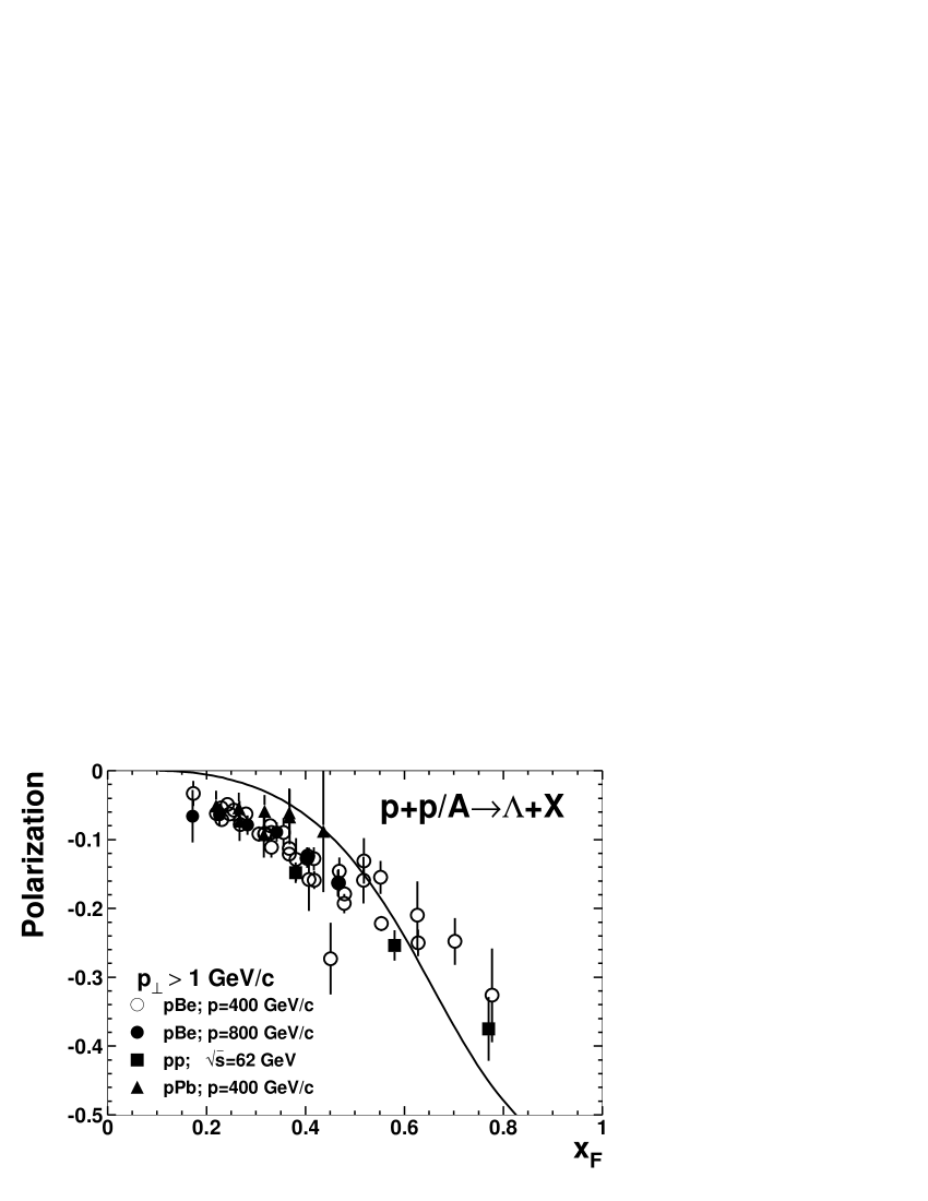
Figure 1: Calculated results for the polarization of $\Lambda$ in $pp$ collisions as a function of $x_{F}$. Data are taken from Refs. Smi87 ; Lun89 ; Ram94 .

Having the $\kappa$’s, we calculate $P_{\Lambda}(x_{F}|s)$ as a function of $x_{F}$. For the unpolarized quark distribution functions, we use the GRV 98 LO set GRV98 . For the unpolarized diquark distribution $f_{D}(x^{P}|q_{v}q_{v})$, we use the parametrization given in Ref. Dug93 . For the unpolarized diquark distribution $f_{D}(x^{T}|q_{s}q_{s})$, we simply use a convolution of $q_{s}(x)$ for the two sea quarks. The obtained results for $P_{\Lambda}(x_{F}|s)$ are given in Fig. 1. The data in the figure are only those for $p_{T}>1$GeV/$c$, because the $C$ that we used in the calculations are determined by $A_{N}$ for the $p_{T}$ interval $0.7<p_{T}<2.0$ GeV/$c$. We see clearly that, as $x_{F}$ changes from 0 to 1, the obtained $P_{\Lambda}(x_{F}|s)$ indeed starts from 0, goes slowly to about $-15\%$ and finally to about $-50\%$ at $x_{F}\to 1$. These qualitative features are the same as we expect from the above-mentioned qualitative analysis and are in good agreement with the data Smi87 ; Lun89 ; Ram94 .

It should be mentioned that, in the calculations presented above, we considered only the associated production of hyperons of group (A), i.e., $(q_{v}q_{v})^{P}+q_{s}^{T}\to H_{i}$, with a pseudo-scalar meson $M$, i.e., $q_{v}^{P}+\bar{q}_{s}^{T}\to M$. It is clear that the associatively produced hadron can also be a vector meson. Taking this into account, we expect that the correlations between the spins of these quarks will be reduced. As a consequence, the polarizations of hyperons from group (A) should be slightly reduced. Since such mesons contribute mainly at large $x_{F}$, this effect should make $|P_{\Lambda}|$ smaller than those presented in Fig. 1 in the large $x_{F}$ region. From the figure, we also see that there is indeed room left for such an effect. Similar effects exist for $pp\to\Sigma^{+}X$ and $\Sigma^{-}p\to\Sigma^{-}(\mbox{or}\ \Xi^{-})X$ that will be discussed in the following. How large this effect can be is determined by the hadronization mechanisms. Presently, we are working on an estimation. The results will be published separately DLfuture .

IV.1.2 $p+p\to\Sigma^{\pm}$(or $\Xi^{0,-}$)$+X$

In a completely similar way, we calculate hyperon polarizations for $pp\to\Sigma^{\pm}\mbox{or}\ \Xi^{0,-})X$. The results are given in the following.

Table 3: Relative weights $w(s_{d},s_{dn}|u_{v}u_{v})$ for the $u_{v}u_{v}$-diquark from proton in different spin states, those for the produced $\Sigma^{+}$, the corresponding $\alpha^{A}_{\Sigma^{+}}$ and total relative weight $w^{A}_{\Sigma^{+}}$.

Possible spin states	$(u_{v}u_{v})_{1,0}s_{s}^{\downarrow}$	$(u_{v}u_{v})_{1,1}s_{s}^{\downarrow}$
$w(s_{d},s_{dn}|u_{v}u_{v})$	$1/3$	$2/3$
Possible products	$\Sigma^{+\downarrow}$	$\Sigma^{+\uparrow}$
$|\langle(u_{v}u_{v})_{s_{d},s_{dn}}s_{s}^{\downarrow}|\Sigma^{+}(s_{n})\rangle|^{2}$	1/3	2/3
The final relative weights	1/9	4/9
The resulted $w_{\Sigma^{+}}^{A}$ and $\alpha^{A}_{\Sigma^{+}}$	$w_{\Sigma^{+}}^{A}=5/9$, $\alpha^{A}_{\Sigma^{+}}=3/5$

For $pp\to\Sigma^{+}X$, there are one contributing process from group (A), i.e., $(u_{v}u_{v})^{P}+s_{s}^{T}\to\Sigma^{+}$ and one from group (B), i.e., $u_{v}^{P}+(u_{s}s_{s})^{T}\to\Sigma^{+}$. The corresponding number densities are given by,

$$D^{A}(x_{F},\Sigma^{+}|s)=\kappa^{d}_{\Sigma^{+}}f_{D}(x^{P}|u_{v}u_{v})s_{s}(x^{T}),$$ (34)

$$D^{B,u}(x_{F},\Sigma^{+}|s)=\kappa u_{v}(x^{P})f_{D}(x^{T}|u_{s}s_{s}),$$ (35)

where $x^{P}\approx x_{F}$ and $x^{T}\approx m_{\Sigma}^{2}/(sx_{F})$. In the case that only $J^{P}=(1/2)^{+}$ hyperon decay is taken into account, there is no contribution from hyperon decay to $\Sigma^{+}$ production. Hence, we have,

$$N(x_{F},\Sigma^{+}|s)=N_{0}(x_{F},\Sigma^{+}|s)+D^{A}(x_{F},\Sigma^{+}|s)+D^{B,u}(x_{F},\Sigma^{+}|s),$$ (36)

$$\Delta N(x_{F},\Sigma^{+}|s)=C[\alpha^{A}_{\Sigma^{+}}D^{A}(x_{F},\Sigma^{+}|s)+t^{F}_{\Sigma^{+},u}D^{B,u}(x_{F},\Sigma^{+}|s)],$$ (37)

where $t^{F}_{\Sigma^{+},u}$ is given in Table 1. $\alpha_{\Sigma^{+}}^{A}$ is calculated in completely the same way as that for $\alpha_{\Lambda}^{A}$ presented in last subsection. The results are given in Table 3. Thus, we have,

$$P_{\Sigma^{+}}(x_{F}|s)=C\frac{\alpha^{A}_{\Sigma^{+}}D^{A}(x_{F},\Sigma^{+}|s)+t^{F}_{\Sigma^{+},u}D^{B,u}(x_{F},\Sigma^{+}|s)}{N_{0}(x_{F},\Sigma^{+}|s)+D^{A}(x_{F},\Sigma^{+}|s)+D^{B,u}(x_{F},\Sigma^{+}|s)}.$$ (38)

The situations for the productions of $\Sigma^{-}$, $\Xi^{0}$ and $\Xi^{-}$ in $pp$ collisions are even simpler: There is no contributing process from group (A) but only one contributing process from (B). When only $J^{P}=(1/2)^{+}$ hyperon decay is taken into account, there is also no contribution from hyperon decay to these hyperons. Hence, we have,

$$P_{\Sigma^{-}}(x_{F}|s)=C\frac{t^{F}_{\Sigma^{-},d}D^{B,d}(x_{F},\Sigma^{-}|s)}{N_{0}(x_{F},\Sigma^{-}|s)+D^{B,d}(x_{F},\Sigma^{-}|s)},$$ (39)

$$P_{\Xi^{0}}(x_{F}|s)=C\frac{t^{F}_{\Xi^{0},u}D^{B,u}(x_{F},\Xi^{0}|s)}{N_{0}(x_{F},\Xi^{0}|s)+D^{B,u}(x_{F},\Xi^{0}|s)},$$ (40)

$$P_{\Xi^{-}}(x_{F}|s)=C\frac{t^{F}_{\Xi^{-},d}D^{B,d}(x_{F},\Xi^{-}|s)}{N_{0}(x_{F},\Xi^{-}|s)+D^{B,d}(x_{F},\Xi^{-}|s)},$$ (41)

where the $t^{F}_{H_{i},f}$’s are given in Table 1,

$$D^{B,d}(x_{F},\Sigma^{-}|s)=\kappa d_{v}(x^{P})f_{D}(x^{T}|d_{s}s_{s}),$$ (42)

and $D^{B,u}(x_{F},\Xi^{0}|s)$ and $D^{B,d}(x_{F},\Xi^{-}|s)$ are given by Eqs. (21) and (22).

From these equations, we can calculate $P_{\Sigma^{\pm}}(x_{F}|s)$ and $P_{\Xi}(x_{F}|s)$ in $pp$ collisions. Just as we mentioned at the end of Subsection III.1, for $pp\to\Sigma^{+}X$, we expect that $D^{A}(x_{F},\Sigma^{+}|s)$ dominates at large $x_{F}$, $D^{B,u}(x_{F},\Sigma^{+}|s)$ plays the dominating role at moderate $x_{F}$. Hence, we expect from Eq. (38) that, $P_{\Sigma^{+}}(x_{F}|s)=0$ for $x_{F}$ near 0, increases to $Ct^{F}_{\Sigma^{+},u}=0.4$ and finally tends to $C\alpha^{A}_{\Sigma^{+}}=0.36$ with increasing $x_{F}$. The situations for $\Sigma^{-}$, $\Xi^{0}$ and $\Xi^{-}$ are even simpler since there is no contributing process from group (A). Here, $N_{0}$ dominates at small $x_{F}$, while $D^{B}$ dominates at large $x_{F}$. We thus expect that $P_{\Sigma^{-}}(x_{F}|s)=0$ for $x_{F}$ near 0 and increases to $Ct^{F}_{\Sigma^{-},d}=0.4$ with increasing $x_{F}$. For $\Xi$, $P_{\Xi}(x_{F}|s)=0$ for $x_{F}$ near 0 and increases to $Ct^{F}_{\Xi,f}=-0.2$ with increasing $x_{F}$. To summarize, we expect that both $P_{\Sigma^{+}}(x_{F}|s)$ and $P_{\Sigma^{-}}(x_{F}|s)$ are positive in sign and increase fast to about $40\%$ with increasing $x_{F}$. On the other hand, both $P_{\Xi^{0}}(x_{F}|s)$ and $P_{\Xi^{-}}(x_{F}|s)$ are negative in sign, and they decrease to $-20\%$ with increasing $x_{F}$. The magnitudes of $P_{\Sigma^{\pm}}$ are expected to be larger than those of $P_{\Xi}$. These qualitative features are in agreement with the available data Wil87 ; Dec83 ; Ramei86 ; Hel83 ; Mor95 ; Dur91 .

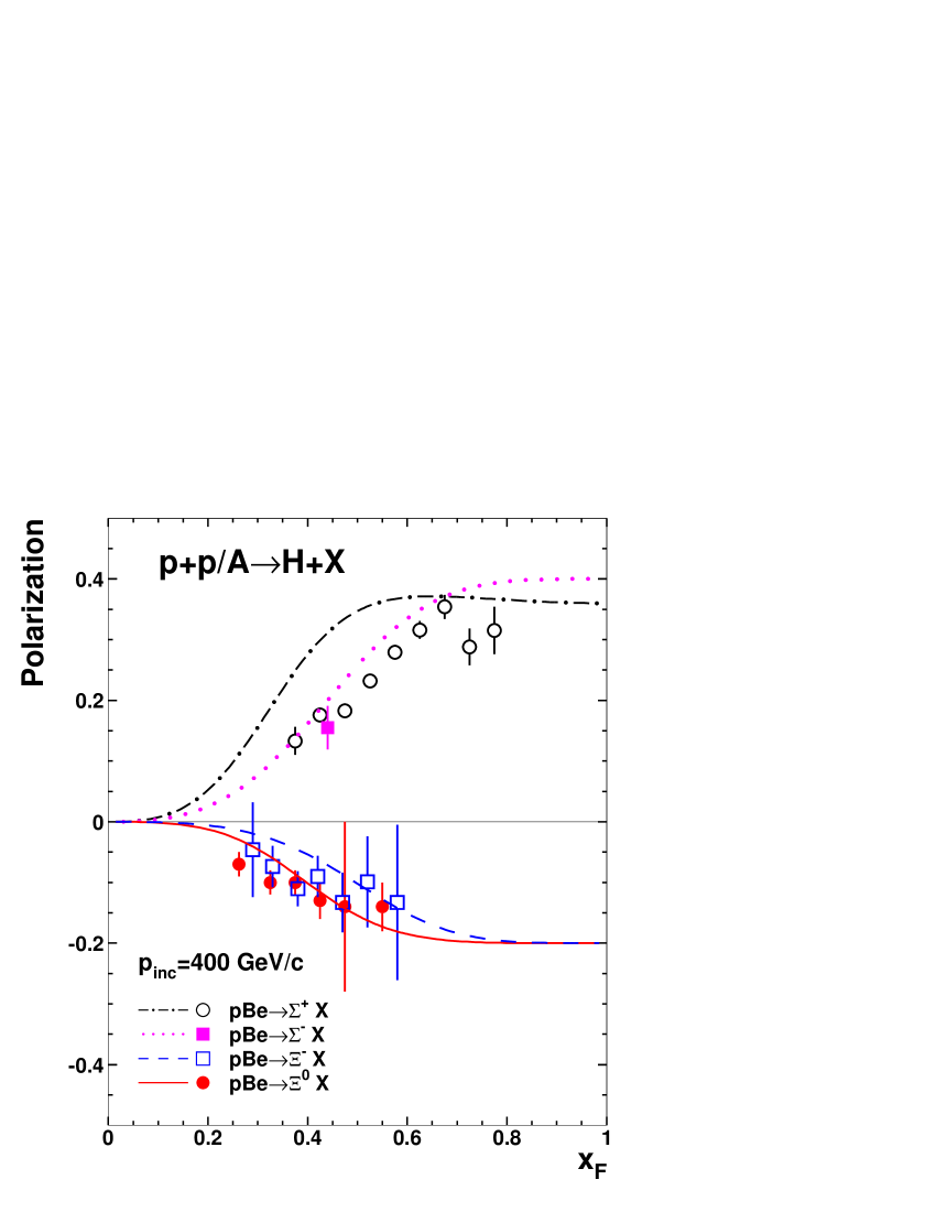
Figure 2: Calculated results for the polarizations of $\Sigma^{\pm}$ and $\Xi^{0,-}$ at $p_{inc}=400\ \mbox{GeV}/c$ in $pp$ collisions as functions of $x_{F}$. Data are taken from Refs. Wil87 ; Dec83 ; Ramei86 ; Hel83 .

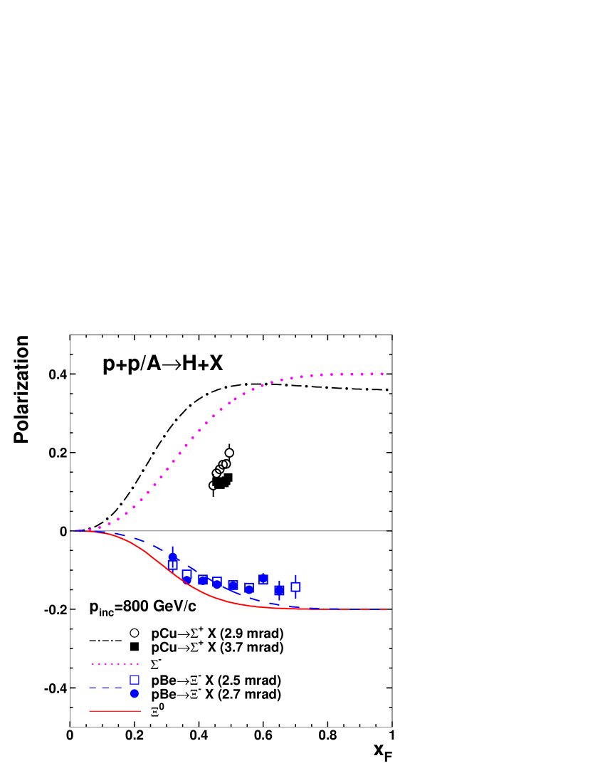
Figure 3: Calculated results for the polarizations of $\Sigma^{\pm}$ and $\Xi^{0,-}$ at $p_{inc}=800\ \mbox{GeV}/c$ in $pp$ collisions as functions of $x_{F}$. Data are taken from Refs. Mor95 ; Dur91 .

We now use Eqs. (38–41) to obtain the numerical results for $P_{\Sigma^{\pm}}(x_{F}|s)$ and $P_{\Xi}(x_{F}|s)$ in $pp$ collisions. The only unknown thing is $N_{0}$ for the corresponding hyperon. As we mentioned earlier in Section III, $N_{0}$ is independent of the polarization properties and can be determined using the data for $N(x_{F},H_{i}|s)$. Since there is no suitable data available for different hyperons, we make the following estimation based on our result on $N_{0}(x_{F},\Lambda|s)$. We simply assume that the $x_{F}$-dependences of all these $N_{0}(x_{F},H_{i}|s)$’s are the same. Hence, we have $N_{0}(x_{F},H_{i}|s)=N_{0}(x_{F},\Lambda|s)\langle n_{H_{i}}\rangle/\langle n_{\Lambda}\rangle$, where $\langle n_{H_{i}}\rangle$ is the average number of $H_{i}$ in the central region. For directly produced hyperons, we take $\langle n_{\Sigma^{+}}\rangle=\langle n_{\Sigma^{-}}\rangle=\langle n_{\Sigma^{0}}\rangle=\langle n^{dir}_{\Lambda}\rangle$, and $\langle n_{\Xi}\rangle=\lambda\langle n_{\Sigma}\rangle$, where $\lambda=0.3$ denotes the strangeness suppression factor. We take $\Sigma^{0}$ and $\Xi$ decays into account, and obtain that $\langle n_{\Lambda}\rangle=(2+2\lambda)\langle n^{dir}_{\Lambda}\rangle$. In this way, we obtain a rough estimation of the $N_{0}(x_{F},H_{i}|s)$. Using this, we obtain the numerical results for $P_{\Sigma^{\pm}(\mbox{or}\ \Xi)}(x_{F}|s)$ at $p_{inc}=400$ GeV/$c$ as shown in Fig. 2, and those at $p_{inc}=800$ GeV/$c$ in Fig. 3. We see that the results show clearly the qualitative features mentioned above and that these features are in agreement with the data Wil87 ; Dec83 ; Ramei86 ; Hel83 ; Mor95 ; Dur91 .

IV.2 Hyperon polarization in $K^{-}+p\to H_{i}+X$

There exist also data for hyperon polarization in $K^{-}p\to\Lambda X$. The data show that $P_{\Lambda}$ in this process is also significantly different from zero for large $x_{F}$. Furthermore, compared with those for $P_{\Lambda}$ in $pp\to\Lambda X$, the data show that $P_{\Lambda}$ in $K^{-}p\to\Lambda X$ has different sign from that for $pp\to\Lambda X$. For $x_{F}$ from 0 to 1, $P_{\Lambda}$ in $K^{-}p\to\Lambda X$ begins with $P_{\Lambda}\approx 0$, increases monotonically to about $40\%$ at $x_{F}\to 1$. Now, we apply the proposed picture to this process, compare the results with the data, and make predictions for other hyperons.

IV.2.1 $K^{-}+p\to\Lambda+X$

Since we have a meson as projectile, there is no contributing process from group (A) to $K^{-}p\to\Lambda X$. There is one contributing process from (B), i.e., $s_{v}^{P}+(u_{s}d_{s})^{T}\to\Lambda$. Thus, we have,

$$D^{B,s}(x_{F},\Lambda|s)=\kappa s^{K}_{v}(x^{P})f_{D}(x^{T}|u_{s}d_{s}),$$ (43)

where $x^{P}\approx x_{F}$ and $x^{T}\approx m_{\Lambda}^{2}/(sx_{F})$. The superscript $K$ for the quark distribution functions denotes that they are for quarks in $K$ meson.

Just as $pp\to\Lambda X$, there are also contributions from hyperon decays to $K^{-}p\to\Lambda X$. In $K^{-}p$ collisions, we have similar contributing processes from group (B) to $\Sigma^{0}$ and $\Xi$ production, i.e., $s_{v}^{P}+(u_{s}d_{s})^{T}\to\Sigma^{0}$, $s_{v}^{P}+(u_{s}s_{s})^{T}\to\Xi^{0}$ and $s_{v}^{P}+(d_{s}s_{s})^{T}\to\Xi^{-}$, respectively. The corresponding number densities are given by,

$$D^{B,s}(x_{F},\Sigma^{0}|s)=\kappa s^{K}_{v}(x^{P})f_{D}(x^{T}|u_{s}d_{s}),$$ (44)

$$D^{B,s}(x_{F},\Xi^{0}|s)=\kappa s^{K}_{v}(x^{P})f_{D}(x^{T}|u_{s}s_{s}),$$ (45)

$$D^{B,s}(x_{F},\Xi^{-}|s)=\kappa s^{K}_{v}(x^{P})f_{D}(x^{T}|d_{s}s_{s}),$$ (46)

respectively.

Hence, we obtain,

$$P_{\Lambda}(x_{F}|s)=C\frac{t^{F}_{\Lambda,s}D^{B,s}(x_{F},\Lambda|s)+\sum_{H_{j}=\Sigma^{0},\Xi^{0},\Xi^{-}}t^{D}_{\Lambda,H_{j}}t^{F}_{H_{j},s}D^{C,H_{j}}(x_{F},\Lambda|s)}{N_{0}(x_{F},\Lambda|s)+D^{B,s}(x_{F},\Lambda|s)+\sum_{H_{j}=\Sigma^{0},\Xi^{0},\Xi^{-}}D^{C,H_{j}}(x_{F},\Lambda|s)},$$ (47)

$$D^{C,H_{j}}(x_{F},\Lambda|s)\approx\frac{m_{H_{j}}}{E_{\Lambda,H_{j}}}D^{B,s}(\frac{m_{H_{j}}x_{F}}{E_{\Lambda,H_{j}}},H_{j}|s),$$ (48)

where the fragmentation spin transfer factors $t^{F}_{H_{j},s}$’s for quark flavor $s$ and different hyperon $H_{j}$ are given in Table 1, and the decay spin transfer factors $t^{D}_{\Lambda,H_{j}}$’s are given in Section III.

Using Eq. (47), we can now calculate $P_{\Lambda}(x_{F}|s)$ in $K^{-}p$ collisions as a function of $x_{F}$. Just as mentioned at the end of Subsection III.1, for $K^{-}p\to\Lambda X$, we expect that $N_{0}$ dominates at small $x_{F}$, while $D^{B}(x_{F},\Lambda|s)$ dominates at large $x_{F}$ since there is no contributing process from group (A). It is clear that $P_{\Lambda}(x_{F}|s)>0$ and, if the decay contribution is neglected, $P_{\Lambda}(x_{F}|s)=0$ for $x_{F}$ near 0 and increases to $Ct^{F}_{\Lambda,s}=C=0.6$ with increasing $x_{F}$. The decay contribution should make $P_{\Lambda}(x_{F}|s)$ slightly less than $C$ at $x_{F}\to 1$ because $0<t^{D}_{\Lambda,H_{j}}t^{F}_{H_{j},s}<t^{F}_{\Lambda,s}$ for all the $H_{j}=\Sigma^{0},\Xi^{0},\Xi^{-}$.

We now use Eq. (47) to obtain the numerical results for $P_{\Lambda}(x_{F}|s)$ in $K^{-}p$ collisions in order to get a more precise feeling of the above-mentioned qualitative features. Here, for the unpolarized quark distribution function of kaon, we use the GRV-P LO set GRV92 for that of pion instead. For $N_{0}(x_{F},H_{i}|s)$ in this process, we simply assume it to be the same as that in $pp$ collisions. The obtained results for $P_{\Lambda}(x_{F}|s)$ are given in Fig. 4. We see that clearly as $x_{F}$ increases from 0 to 1, the obtained $P_{\Lambda}(x_{F}|s)$ starts from 0 and increases to about $40\%$ at $x_{F}\to 1$. These qualitative features are in good agreement with the data Gou86 ; Fac79 ; Gra78 ; Abr76 ; Bau79 .

IV.2.2 $K^{-}+p\to\Sigma^{\pm}$ (or $\Xi^{0,-}$)$+X$

Similar to $K^{-}p\to\Lambda X$ in $K^{-}p$ collisions, there is also only one contributing process from group (B) to the production of each of these hyperons. For $\Sigma^{+}$ and $\Sigma^{-}$, they are $s_{v}^{P}+(u_{s}u_{s})^{T}\to\Sigma^{+}$ and $s_{v}^{P}+(d_{s}d_{s})^{T}\to\Sigma^{-}$, respectively. The corresponding number densities are given by,

$$D^{B,s}(x_{F},\Sigma^{+}|s)=\kappa s^{K}_{v}(x^{P})f_{D}(x^{T}|u_{s}u_{s}),$$ (49)

$$D^{B,s}(x_{F},\Sigma^{-}|s)=\kappa s^{K}_{v}(x^{P})f_{D}(x^{T}|d_{s}d_{s}),$$ (50)

respectively. The contributing processes from (B) to $\Xi$ production have been given in the last subsection and their corresponding number densities are given by Eqs. (45) and (46). Thus, we have,

$$P_{\Sigma^{+}}(x_{F}|s)=C\frac{t^{F}_{\Sigma^{+},s}D^{B,s}(x_{F},\Sigma^{+}|s)}{N_{0}(x_{F},\Sigma^{+}|s)+D^{B,s}(x_{F},\Sigma^{+}|s)},$$ (51)

$$P_{\Sigma^{-}}(x_{F}|s)=C\frac{t^{F}_{\Sigma^{-},s}D^{B,s}(x_{F},\Sigma^{-}|s)}{N_{0}(x_{F},\Sigma^{-}|s)+D^{B,s}(x_{F},\Sigma^{-}|s)},$$ (52)

$$P_{\Xi^{0}}(x_{F}|s)=C\frac{t^{F}_{\Xi^{0},s}D^{B,s}(x_{F},\Xi^{0}|s)}{N_{0}(x_{F},\Xi^{0}|s)+D^{B,s}(x_{F},\Xi^{0}|s)},$$ (53)

$$P_{\Xi^{-}}(x_{F}|s)=C\frac{t^{F}_{\Xi^{-},s}D^{B,s}(x_{F},\Xi^{-}|s)}{N_{0}(x_{F},\Xi^{-}|s)+D^{B,s}(x_{F},\Xi^{-}|s)},$$ (54)

where the $t^{F}_{H_{i},s}$’s are given in Table 1.

It is also clear that, for the productions of these hyperons, $N_{0}$ dominates at small $x_{F}$, while $D^{B}$ plays the dominating role at large $x_{F}$. We expect that, for $\Sigma^{\pm}$ in $K^{-}p$ collisions, $P_{\Sigma^{\pm}}(x_{F}|s)=0$ for $x_{F}$ near 0 and decreases to $Ct^{F}_{\Sigma,s}=-0.2$ with increasing $x_{F}$. For $K^{-}p\to\Xi X$, $P_{\Xi}(x_{F}|s)=0$ for $x_{F}$ near 0 and increases to $Ct^{F}_{\Xi,s}=0.4$ with increasing $x_{F}$. This means that $P_{\Sigma^{\pm}}(x_{F}|s)$ is negative in sign and decreases to $-20\%$ with increasing $x_{F}$, while $P_{\Xi}(x_{F}|s)$ is positive in sign and increases fast to $40\%$ with increasing $x_{F}$. The magnitudes of $P_{\Sigma^{\pm}}$ should be smaller than those of $P_{\Xi}$. These qualitative features are different from those for $pp$ collisions and can be checked by future experiments.

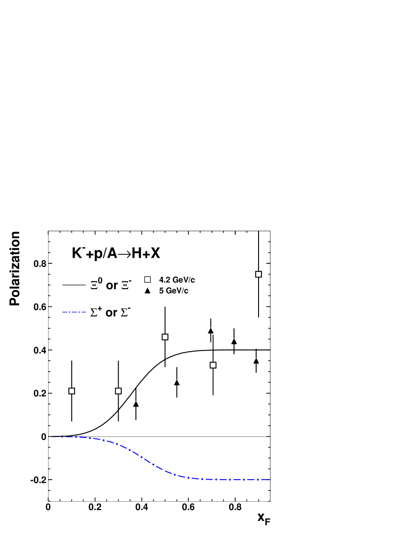
Figure 5: Calculated results for the polarizations of $\Sigma^{\pm}$ and $\Xi^{0,-}$ in $K^{-}p$ collisions as functions of $x_{F}$. Data for $\Xi^{-}$ are taken from Refs. Gan77 ; Ben85 .

By using Eqs. (51–54), we also obtain the numerical results for $P_{\Sigma^{\pm}}(x_{F}|s)$ and $P_{\Xi}(x_{F}|s)$ as functions of $x_{F}$ in $K^{-}p$ collisions. They are given in Fig. 5. At present, there are only data available for $\Xi^{-}$ Gan77 ; Ben85 among these hyperons. We see that the results show clearly the qualitative features mentioned above and that those for $\Xi^{-}$ are consistent with the available data. They all can be further checked by further experiments.

IV.3 Hyperon polarization in $\pi^{\pm}+p\to H_{i}+X$

Now, we apply the proposed picture to $\pi^{\pm}p$ collisions. From the isospin symmetry, we obtain that $P_{\Lambda}$ in $\pi^{+}p\to\Lambda X$ is the same as that in $\pi^{-}p\to\Lambda X$, $P_{\Sigma^{+}}$ and $P_{\Xi^{0}}$ in $\pi^{+}p$ collisions are the same as $P_{\Sigma^{-}}$ and $P_{\Xi^{-}}$ in $\pi^{-}p$ collisions, respectively. So we only give the calculations for $\pi^{-}+p\to H_{i}+X$.

IV.3.1 $\pi^{-}+p\to\Lambda+X$

Similar to $K^{-}p\to\Lambda X$, there is also no contributing process from group (A) to $\pi^{-}p\to\Lambda X$. There is one contributing process from (B), i.e., $d_{v}^{P}+(u_{s}s_{s})^{T}\to\Lambda$. Thus, we have,

$$D^{B,d}(x_{F},\Lambda|s)=\kappa d^{\pi}_{v}(x^{P})f_{D}(x^{T}|u_{s}s_{s}),$$ (55)

where $x^{P}\approx x_{F}$ and $x^{T}\approx m_{\Lambda}^{2}/(sx_{F})$.

Just as $pp\to\Lambda X$, there are also contributions from hyperon decays to $\pi^{-}p\to\Lambda X$. In $\pi^{-}p$ collisions, we have similar contributing processes from group (B) to $\Sigma^{0}$ and $\Xi^{-}$ production, i.e., $d_{v}^{P}+(u_{s}s_{s})^{T}\to\Sigma^{0}$ and $d_{v}^{P}+(s_{s}s_{s})^{T}\to\Xi^{-}$, respectively. Their corresponding number densities are given by,

$$D^{B,d}(x_{F},\Sigma^{0}|s)=\kappa d^{\pi}_{v}(x^{P})f_{D}(x^{T}|u_{s}s_{s}),$$ (56)

$$D^{B,d}(x_{F},\Xi^{-}|s)=\kappa d^{\pi}_{v}(x^{P})f_{D}(x^{T}|s_{s}s_{s}),$$ (57)

respectively.

Finally, we have,

$$P_{\Lambda}(x_{F}|s)=\frac{C\sum_{H_{j}=\Sigma^{0},\Xi^{-}}t^{D}_{\Lambda,H_{j}}t^{F}_{H_{j},d}D^{C,H_{j}}(x_{F},\Lambda|s)}{N_{0}(x_{F},\Lambda|s)+D^{B,d}(x_{F},\Lambda|s)+\sum_{H_{j}=\Sigma^{0},\Xi^{-}}D^{C,H_{j}}(x_{F},\Lambda|s)},$$ (58)

$$D^{C,H_{j}}(x_{F},\Lambda|s)\approx\frac{m_{H_{j}}}{E_{\Lambda,H_{j}}}D^{B,d}(\frac{m_{H_{j}}x_{F}}{E_{\Lambda,H_{j}}},H_{j}|s),$$ (59)

where the fragmentation spin transfer factors $t^{F}_{H_{j},d}$’s for quark flavor $d$ and different hyperon $H_{j}$ are given in Table 1, and the decay spin transfer factors $t^{D}_{\Lambda,H_{j}}$’s are given in Section III.

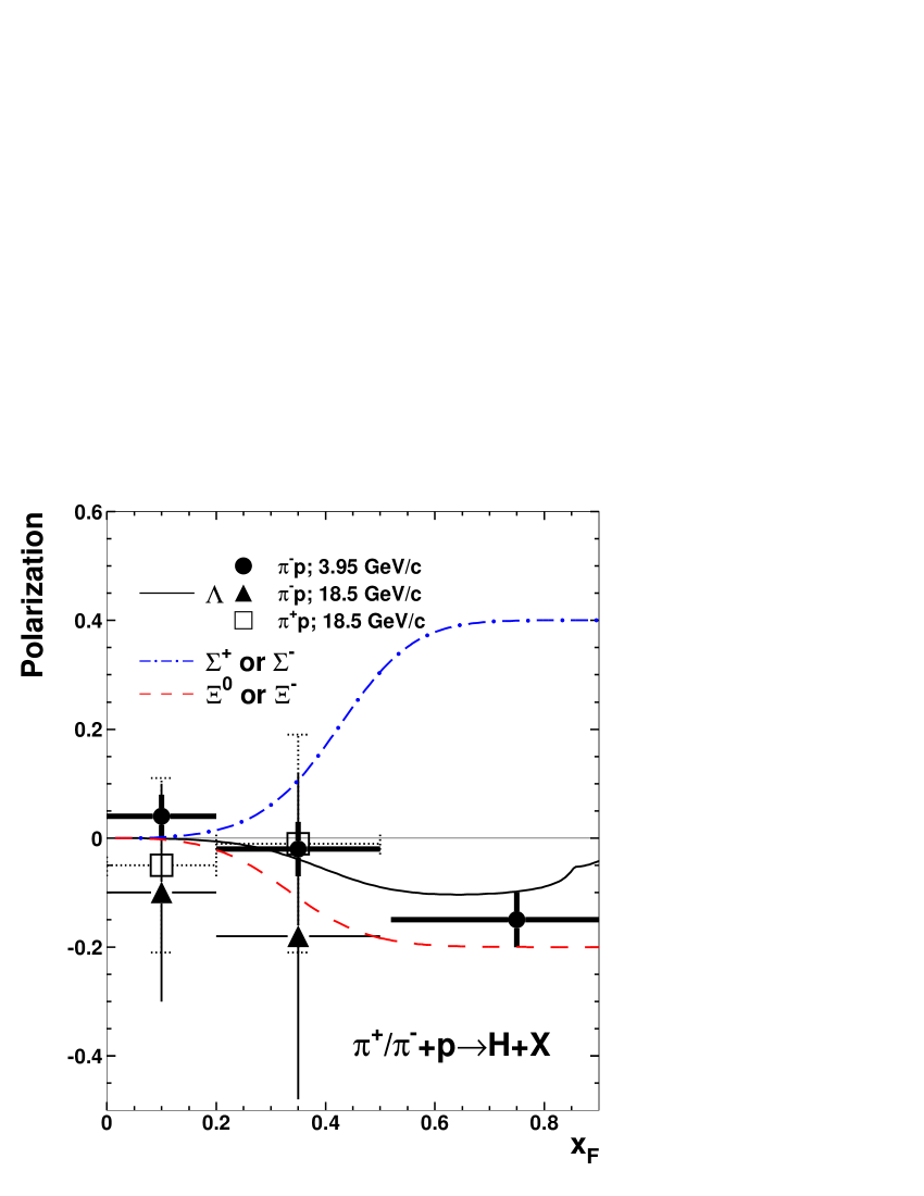
Figure 6: Calculated results for the polarizations of $\Lambda$, $\Sigma^{\pm}$ and $\Xi^{0,-}$ in $\pi p$ collisions as functions of $x_{F}$. Data for $\Lambda$ are taken from Refs. Ade84 ; Stu74 .

From Eq. (58), we see immediately that, since $t^{F}_{\Lambda,d}=0$, $P_{\Lambda}(x_{F}|s)$ in $\pi p\to\Lambda X$ should be equal to zero if the decay contributions are neglected. The nonzero $P_{\Lambda}$ in this process comes purely from the decays of heavier hyperons. Taking these decay contributions into account, we expect a small and negative $P_{\Lambda}(x_{F}|s)$ at large $x_{F}$ because $Ct^{D}_{\Lambda,\Sigma^{0}}t^{F}_{\Sigma^{0},d}=-0.13$, and $Ct^{D}_{\Lambda,\Xi}t^{F}_{\Xi^{-},d}=-0.18$. The numerical results obtained from Eq. (58) are given in Fig. 6. In the calculations, we use the GRV-P LO set GRV92 for the unpolarized quark distribution function of pion and simply assume $N_{0}(x_{F},H_{i}|s)$ in this process to be the same as that in $pp$ collisions. We clearly see that, as $x_{F}$ goes from 0 to 1, the obtained $P_{\Lambda}(x_{F}|s)$ starts from 0 and decreases to about $-10\%$ at large $x_{F}$. These qualitative features are in agreement with the data Ade84 ; Stu74 .

IV.3.2 $\pi^{-}+p\to\Sigma^{-}$ (or $\Xi^{-}$)$+X$

In $\pi^{-}p$ collisions, there is one contributing process from group (B) to the production of $\Sigma^{-}$ and $\Xi^{-}$. For $\Sigma^{-}$, it is $d_{v}^{P}+(d_{s}s_{s})^{T}\to\Sigma^{-}$. The corresponding number density is given by,

$$D^{B,d}(x_{F},\Sigma^{-}|s)=\kappa d^{\pi}_{v}(x^{P})f_{D}(x^{T}|d_{s}s_{s}).$$ (60)

The contributing process from (B) to $\Xi^{-}$ production has been given in the last subsection and its corresponding number density is given by Eq. (57). Thus, we have,

$$P_{\Sigma^{-}}(x_{F}|s)=C\frac{t^{F}_{\Sigma^{-},d}D^{B,d}(x_{F},\Sigma^{-}|s)}{N_{0}(x_{F},\Sigma^{-}|s)+D^{B,d}(x_{F},\Sigma^{-}|s)},$$ (61)

$$P_{\Xi^{-}}(x_{F}|s)=C\frac{t^{F}_{\Xi^{-},d}D^{B,d}(x_{F},\Xi^{-}|s)}{N_{0}(x_{F},\Xi^{-}|s)+D^{B,d}(x_{F},\Xi^{-}|s)}.$$ (62)

As given in Table 1, $t^{F}_{\Sigma^{-},d}=2/3$, and $t^{F}_{\Xi^{-},d}=-1/3$. We thus expect that $P_{\Sigma^{-}}(x_{F}|s)=0$ for $x_{F}$ near 0 and increases to $Ct^{F}_{\Sigma^{-},d}=0.4$ with increasing $x_{F}$. For $\Xi^{-}$, $P_{\Xi}(x_{F}|s)=0$ for $x_{F}$ near 0 and decreases to $Ct^{F}_{\Xi^{-},d}=-0.2$ with increasing $x_{F}$. This implies that $P_{\Sigma^{-}}(x_{F}|s)$ is positive in sign and increases fast to $40\%$ with increasing $x_{F}$, while $P_{\Xi^{-}}(x_{F}|s)$ is negative in sign and decreases to $-20\%$ with increasing $x_{F}$. The magnitude of $P_{\Sigma^{-}}$ should be larger than that of $P_{\Xi^{-}}$.

Using these equations, We obtain the numerical results for $P_{\Sigma^{-}}(x_{F}|s)$ and $P_{\Xi^{-}}(x_{F}|s)$ in $\pi^{-}p$ collisions as shown in Fig. 6. We see that the results show clearly the qualitative features mentioned above. These features can be tested by future experiments.

IV.4 Hyperon polarization in $\Sigma^{-}+p\to H_{i}+X$

It is interesting to note that experiments on hyperon polarizations in reactions using $\Sigma^{-}$ beam have also been carried out by the WA89 Collaboration at CERN. Some of the results have already been published WA89-95 and more results are coming. We now apply the proposed picture to this process.

IV.4.1 $\Sigma^{-}+p\to\Lambda+X$

Similar to $pp\to\Lambda X$, for $\Sigma^{-}p\to\Lambda X$, there are one contributing process from group (A), i.e., $(d_{v}s_{v})^{P}+u_{s}^{T}\to\Lambda$ and two contributing processes from (B), i.e., $d_{v}^{P}+(u_{s}s_{s})^{T}\to\Lambda$ and $s_{v}^{P}+(u_{s}d_{s})^{T}\to\Lambda$. Thus, we have,

$$D^{A}(x_{F},\Lambda|s)=\kappa_{\Lambda}^{d}f^{\Sigma^{-}}_{D}(x^{P}|d_{v}s_{v})u_{s}(x^{T}),$$ (63)

$$D^{B,d}(x_{F},\Lambda|s)=\kappa d^{\Sigma^{-}}_{v}(x^{P})f_{D}(x^{T}|u_{s}s_{s}),$$ (64)

$$D^{B,s}(x_{F},\Lambda|s)=\kappa s^{\Sigma^{-}}_{v}(x^{P})f_{D}(x^{T}|u_{s}d_{s}).$$ (65)

There are also contributions from hyperon decays to $\Sigma^{-}p\to\Lambda X$. For $\Sigma^{-}p\to\Sigma^{0}(\mbox{or}\ \Xi^{-})X$, we have similar contributing processes from groups (A) and (B) as those for $\Sigma^{-}p\to\Lambda X$. For $\Sigma^{0}$, they are $(d_{v}s_{v})^{P}+u_{s}^{T}\to\Sigma^{0}$, $d_{v}^{P}+(u_{s}s_{s})^{T}\to\Sigma^{0}$ and $s_{v}^{P}+(u_{s}d_{s})^{T}\to\Sigma^{0}$. The number densities of $\Sigma^{0}$ from these processes are given by,

$$D^{A}(x_{F},\Sigma^{0}|s)=\kappa_{\Sigma^{0}}^{d}f^{\Sigma^{-}}_{D}(x^{P}|d_{v}s_{v})u_{s}(x^{T}),$$ (66)

$$D^{B,d}(x_{F},\Sigma^{0}|s)=\kappa d^{\Sigma^{-}}_{v}(x^{P})f_{D}(x^{T}|u_{s}s_{s}),$$ (67)

$$D^{B,s}(x_{F},\Sigma^{0}|s)=\kappa s^{\Sigma^{-}}_{v}(x^{P})f_{D}(x^{T}|u_{s}d_{s}),$$ (68)

respectively.

For $\Xi^{-}$, they are $(d_{v}s_{v})^{P}+s_{s}^{T}\to\Xi^{-}$, $d_{v}^{P}+(s_{s}s_{s})^{T}\to\Xi^{-}$ and $s_{v}^{P}+(d_{s}s_{s})^{T}\to\Xi^{-}$. The corresponding number densities are given by,

$$D^{A}(x_{F},\Xi^{-}|s)=\kappa_{\Xi^{-}}^{d}f^{\Sigma^{-}}_{D}(x^{P}|d_{v}s_{v})s_{s}(x^{T}),$$ (69)

$$D^{B,d}(x_{F},\Xi^{-}|s)=\kappa d^{\Sigma^{-}}_{v}(x^{P})f_{D}(x^{T}|s_{s}s_{s}),$$ (70)

$$D^{B,s}(x_{F},\Xi^{-}|s)=\kappa s^{\Sigma^{-}}_{v}(x^{P})f_{D}(x^{T}|d_{s}s_{s}),$$ (71)

respectively.

For $\Sigma^{-}p\to\Xi^{0}X$, there is one contributing process from (B), i.e., $s_{v}^{P}+(u_{s}s_{s})^{T}\to\Xi^{0}$. The corresponding number density is given by,

$$D^{B,s}(x_{F},\Xi^{0}|s)=\kappa s^{\Sigma^{-}}_{v}(x^{P})f_{D}(x^{T}|u_{s}s_{s}).$$ (72)

Thus, we obtain that,

$$N(x_{F},\Lambda|s)=N_{0}(x_{F},\Lambda|s)+D^{A}(x_{F},\Lambda|s)+\sum_{f=d,s}D^{B,f}(x_{F},\Lambda|s)+\sum_{H_{j}=\Sigma^{0},\Xi^{0},\Xi^{-}}D^{C,H_{j}}(x_{F},\Lambda|s),$$ (73)

$$D^{C,\Sigma^{0}}(x_{F},\Lambda|s)\approx\frac{m_{\Sigma}}{E_{\Lambda,\Sigma^{0}}}[D^{A}(\frac{m_{\Sigma}x_{F}}{E_{\Lambda,\Sigma^{0}}},\Sigma^{0}|s)+\sum_{f=d,s}{D^{B,f}(\frac{m_{\Sigma}x_{F}}{E_{\Lambda,\Sigma^{0}}},\Sigma^{0}|s)}],$$ (74)

$$D^{C,\Xi^{0}}(x_{F},\Lambda|s)\approx\frac{m_{\Xi}}{E_{\Lambda,\Xi}}D^{B,s}(\frac{m_{\Xi}x_{F}}{E_{\Lambda,\Xi}},\Xi^{0}|s),$$ (75)

$$D^{C,\Xi^{-}}(x_{F},\Lambda|s)\approx\frac{m_{\Xi}}{E_{\Lambda,\Xi}}[D^{A}(\frac{m_{\Xi}x_{F}}{E_{\Lambda,\Xi}},\Xi^{-}|s)+\sum_{f=d,s}{D^{B,f}(\frac{m_{\Xi}x_{F}}{E_{\Lambda,\Xi}},\Xi^{-}|s)}].$$ (76)

Table 4: Relative weights $w(s_{d},s_{dn}|d_{v}s_{v})$ for the $d_{v}s_{v}$-diquark from $\Sigma^{-}$ in different spin states, those for the produced $\Lambda$ and $\Sigma^{0}$, the corresponding $\alpha^{A}_{\Lambda}$ and $\alpha^{A}_{\Sigma^{0}}$ and the total weights $w^{A}_{\Lambda}$ and $w^{A}_{\Sigma^{0}}$.

Possible spin states	$(d_{v}s_{v})_{0,0}u_{s}^{\downarrow}$		$(d_{v}s_{v})_{1,0}u_{s}^{\downarrow}$		$(d_{v}s_{v})_{1,1}u_{s}^{\downarrow}$
$w(s_{d},s_{dn}|d_{v}s_{v})$	$3/4$		$1/12$		$1/6$
Possible products	$\Lambda^{\downarrow}$	$\Sigma^{0\downarrow}$	$\Lambda^{\downarrow}$	$\Sigma^{0\downarrow}$	$\Lambda^{\uparrow}$	$\Sigma^{0\uparrow}$
$|\langle(q_{v}q_{v})_{s_{d},s_{dn}}q_{s}^{\downarrow}|H_{i}(s_{n})\rangle|^{2}$	1/4	3/4	1/4	$1/12$	1/2	$1/6$
The final relative weights	3/16	9/16	1/48	$1/144$	1/12	$1/36$
The resulted $w_{Hi}^{A}$ and $\alpha^{A}_{Hi}$	$\Lambda$: $7/24$,  $-3/7$;			$\Sigma^{0}$: $43/72$,  $-39/43$

Table 5: Relative weights $w(s_{d},s_{dn}|d_{v}s_{v})$ for the $d_{v}s_{v}$-diquark from $\Sigma^{-}$ in different spin states, those for the produced $\Xi^{-}$, the corresponding $\alpha^{A}_{\Xi^{-}}$ and the total weight $w^{A}_{\Xi^{-}}$.

Possible spin states	$(d_{v}s_{v})_{0,0}s_{s}^{\downarrow}$	$(d_{v}s_{v})_{1,0}s_{s}^{\downarrow}$	$(d_{v}s_{v})_{1,1}s_{s}^{\downarrow}$
$w(s_{d},s_{dn}|d_{v}s_{v})$	$3/4$	$1/12$	$1/6$
Possible products	$\Xi^{-\downarrow}$	$\Xi^{-\downarrow}$	$\Xi^{-\uparrow}$
$|\langle(q_{v}q_{v})_{s_{d},s_{dn}}q_{s}^{\downarrow}|H_{i}(s_{n})\rangle|^{2}$	3/4	1/12	1/6
The final relative weights	9/16	1/144	1/36
The resulted $w_{Hi}^{A}$ and $\alpha^{A}_{Hi}$	$\Xi^{-}$: $43/72$,  $-39/43$

In the same way as that of $pp\to\Lambda X$, we calculate $w^{A}_{\Lambda}$, the total relative weight for the production of $\Lambda$ from group (A), and $\alpha_{\Lambda}^{A}$. The results are shown in Table 4. Similarly, we obtain the corresponding results for $\Sigma^{0}$ production as shown in the same table and those for $\Xi^{-}$ production as shown in Table 5. From these results, we obtain,

$$\Delta N(x_{F},\Lambda|s)=C\alpha^{A}_{\Lambda}D^{A}(x_{F},\Lambda|s)+Ct^{F}_{\Lambda,s}D^{B,s}(x_{F},\Lambda|s)+\sum_{H_{j}=\Sigma^{0},\Xi^{0},\Xi^{-}}\Delta D^{C,H_{j}}(x_{F},\Lambda|s),$$ (77)

$$\Delta D^{C,\Sigma^{0}}(x_{F},\Lambda|s)\approx Ct^{D}_{\Lambda,\Sigma^{0}}\frac{m_{\Sigma}}{E_{\Lambda,\Sigma^{0}}}[\alpha^{A}_{\Sigma^{0}}D^{A}(\frac{m_{\Sigma}x_{F}}{E_{\Lambda,\Sigma^{0}}},\Sigma^{0}|s)+\sum_{f=d,s}{t^{F}_{\Sigma^{0},f}D^{B,f}(\frac{m_{\Sigma}x_{F}}{E_{\Lambda,\Sigma^{0}}},\Sigma^{0}|s)}],$$ (78)

$$\Delta D^{C,\Xi^{0}}(x_{F},\Lambda|s)\approx Ct^{D}_{\Lambda,\Xi}t^{F}_{\Xi^{0},s}\frac{m_{\Xi}}{E_{\Lambda,\Xi}}D^{B,s}(\frac{m_{\Xi}x_{F}}{E_{\Lambda,\Xi}},\Xi^{0}|s),$$ (79)

$$\Delta D^{C,\Xi^{-}}(x_{F},\Lambda|s)\approx Ct^{D}_{\Lambda,\Xi}\frac{m_{\Xi}}{E_{\Lambda,\Xi}}[\alpha^{A}_{\Xi^{-}}D^{A}(\frac{m_{\Xi}x_{F}}{E_{\Lambda,\Xi}},\Xi^{-}|s)+\sum_{f=d,s}{t^{F}_{\Xi^{-},f}D^{B,f}(\frac{m_{\Xi}x_{F}}{E_{\Lambda,\Xi}},\Xi^{-}|s)}],$$ (80)

where the fragmentation spin transfer factors $t^{F}_{H_{j},f}$’s for different quark flavor $f$ and different hyperon $H_{j}$ are given in Table 1, and the decay spin transfer factors $t^{D}_{\Lambda,H_{j}}$’s are given in Section III.

Using the results given by Eqs. (63–80), we can now calculate $P_{\Lambda}(x_{F}|s)$ in $\Sigma^{-}p$ collisions as a function of $x_{F}$. Between the two contributing processes from (B), the contribution from $s_{v}^{P}+(u_{s}d_{s})^{T}\to\Lambda$ is more important than that from $d_{v}^{P}+(u_{s}s_{s})^{T}\to\Lambda$ due to the strangeness suppression in the sea quarks of the target. We note that $\alpha^{A}_{\Lambda}=-3/7$, $t^{F}_{\Lambda,d}=0$, and $t^{F}_{\Lambda,s}=1$. Hence, if we neglect the decay contributions, we expect that, for $x_{F}$ increasing from 0 to 1, $P_{\Lambda}(x_{F}|s)$ starts from 0, increases to some positive value, then decreases to $C\alpha^{A}_{\Lambda}=-3C/7$ at $x_{F}\to 1$. We also note that $\alpha^{A}_{\Sigma^{0}}=-39/43$ which is large in magnitude and has the same sign as $\alpha^{A}_{\Lambda}$. This is quite different from the situation in $pp\to\Lambda X$ where $\alpha^{A}_{\Sigma^{0}}$ has different sign and smaller magnitude compared to $\alpha^{A}_{\Lambda}$. Since the decay spin transfer factor $t^{D}_{\Lambda,\Sigma^{0}}=-1/3$, we thus expect a very significant contribution from the $\Sigma^{0}$ decay to $P_{\Lambda}$ in $\Sigma^{-}p\to\Lambda X$, and this contribution cancels that from the directly produced $\Lambda$ at large $x_{F}$. As a consequence, taking the decay contributions into account, in particular the significant contribution from $\Sigma^{0}\to\Lambda\gamma$, we expect that, for $x_{F}$ going from 0 to 1, $P_{\Lambda}(x_{F}|s)$ starts from 0, increases slowly to some positive value at moderate $x_{F}$, and then begins to decrease at some $x_{F}$ and finally reaches some negative value but the magnitude less than $3C/7$ at $x_{F}\to 1$.

To get some quantitative feeling, we now use Eqs. (63–80) to calculate $P_{\Lambda}(x_{F}|s)$ in $\Sigma^{-}p$ collisions numerically. Since our purpose is to get a feeling of the $x_{F}$-dependence of $P_{\Lambda}(x_{F}|s)$, we simply make the following simplifications. For the unpolarized quark distribution functions in $\Sigma^{-}$, we approximately use those in proton GRV98 to replace them. For $N_{0}(x_{F},H_{i}|s)$, we take it as the same as that in $pp$ collisions. The obtained numerical results for $P_{\Lambda}(x_{F}|s)$ are given in Fig. 7. We see clearly that, as $x_{F}$ increases from 0 to 1, the obtained $P_{\Lambda}(x_{F}|s)$ first increases from 0 to some positive value, then decreases even to negative at $x_{F}\to 1$. These qualitative features are just those expected above. They can be checked by further experiments.

IV.4.2 $\Sigma^{-}+p\to\Sigma^{\pm}$ (or $\Xi^{0,-}$)$+X$

Table 6: Relative weights $w(s_{d},s_{dn}|d_{v}s_{v})$ for the $d_{v}s_{v}$-diquark from $\Sigma^{-}$ in different spin states, those for the produced $\Sigma^{-}$, the corresponding $\alpha^{A,ds}_{\Sigma^{-}}$ and the total weight $w^{A,ds}_{\Sigma^{-}}$.

Possible spin states	$(d_{v}s_{v})_{0,0}d_{s}^{\downarrow}$	$(d_{v}s_{v})_{1,0}d_{s}^{\downarrow}$	$(d_{v}s_{v})_{1,1}d_{s}^{\downarrow}$
$w(s_{d},s_{dn}|d_{v}s_{v})$	$3/4$	$1/12$	$1/6$
Possible products	$\Sigma^{-\downarrow}$	$\Sigma^{-\downarrow}$	$\Sigma^{-\uparrow}$
$|\langle(q_{v}q_{v})_{s_{d},s_{dn}}q_{s}^{\downarrow}|H_{i}(s_{n})\rangle|^{2}$	3/4	1/12	1/6
The final relative weights	9/16	1/144	1/36
The resulted $w_{Hi}^{A}$ and $\alpha^{A}_{Hi}$	$\Sigma^{-}$: $43/72$,  $-39/43$

Table 7: Relative weights $w(s_{d},s_{dn}|d_{v}d_{v})$ for the $d_{v}d_{v}$-diquark from $\Sigma^{-}$ in different spin states, those for the produced $\Sigma^{-}$, the corresponding $\alpha^{A,dd}_{\Sigma^{-}}$ and the total weight $w^{A,dd}_{\Sigma^{-}}$.

Possible spin states	$(d_{v}d_{v})_{0,0}s_{s}^{\downarrow}$	$(d_{v}d_{v})_{1,0}s_{s}^{\downarrow}$	$(d_{v}d_{v})_{1,1}s_{s}^{\downarrow}$
$w(s_{d},s_{dn}|d_{v}d_{v})$	0	$1/3$	$2/3$
Possible products	$\Sigma^{-\downarrow}$	$\Sigma^{-\downarrow}$	$\Sigma^{-\uparrow}$
$|\langle(q_{v}q_{v})_{s_{d},s_{dn}}q_{s}^{\downarrow}|H_{i}(s_{n})\rangle|^{2}$	—	1/3	2/3
The final relative weights	—	1/9	4/9
The resulted $w_{Hi}^{A}$ and $\alpha^{A}_{Hi}$	$\Sigma^{-}$: 5/9,  3/5

First, we look at $\Sigma^{-}$ production in $\Sigma^{-}p$ collisions. For $\Sigma^{-}p\to\Sigma^{-}X$, there are two contributing processes from group (A), i.e., $(d_{v}s_{v})^{P}+d_{s}^{T}\to\Sigma^{-}$ and $(d_{v}d_{v})^{P}+s_{s}^{T}\to\Sigma^{-}$ and two from (B), i.e., $d_{v}^{P}+(d_{s}s_{s})^{T}\to\Sigma^{-}$ and $s_{v}^{P}+(d_{s}d_{s})^{T}\to\Sigma^{-}$. The corresponding number densities are given by,

$$D^{A,ds}(x_{F},\Sigma^{-}|s)=\kappa^{d}_{\Sigma^{-}}f^{\Sigma^{-}}_{D}(x^{P}|d_{v}s_{v})d_{s}(x^{T}),$$ (81)

$$D^{A,dd}(x_{F},\Sigma^{-}|s)=\kappa^{d}_{\Sigma^{-}}f^{\Sigma^{-}}_{D}(x^{P}|d_{v}d_{v})s_{s}(x^{T}),$$ (82)

$$D^{B,d}(x_{F},\Sigma^{-}|s)=\kappa d^{\Sigma^{-}}_{v}(x^{P})f_{D}(x^{T}|d_{s}s_{s}),$$ (83)

$$D^{B,s}(x_{F},\Sigma^{-}|s)=\kappa s^{\Sigma^{-}}_{v}(x^{P})f_{D}(x^{T}|d_{s}d_{s}).$$ (84)

Hence, we have,

$$P_{\Sigma^{-}}(x_{F}|s)=C\frac{\sum_{f=ds,dd}{\alpha^{A,f}_{\Sigma^{-}}D^{A,f}(x_{F},\Sigma^{-}|s)}+\sum_{f=d,s}{t^{F}_{\Sigma^{-},f}D^{B,f}(x_{F},\Sigma^{-}|s)}}{N_{0}(x_{F},\Sigma^{-}|s)+\sum_{f=ds,dd}{D^{A,f}(x_{F},\Sigma^{-}|s)}+\sum_{f=d,s}{D^{B,f}(x_{F},\Sigma^{-}|s)}},$$ (85)

where $t^{F}_{\Sigma^{-},f}$’s are given in Table 1, $\alpha^{A,f}_{\Sigma^{-}}$ and other related quantities describing $\Sigma^{-}$ from the two contributing processes from (A) are shown in Table 6 and 7, respectively.

Because of the strangeness suppression in the sea quarks of the target, we expect that the most important contributing process to the production of $\Sigma^{-}$ from (A) is $(d_{v}s_{v})^{P}+d_{s}^{T}\to\Sigma^{-}$ and that from (B) is $s_{v}^{P}+(d_{s}d_{s})^{T}\to\Sigma^{-}$. From Tables 6 and 1, we see that $\alpha^{A,ds}_{\Sigma^{-}}=-39/43$, and $t^{F}_{\Sigma^{-},s}=-1/3$. Both of them contribute negatively to the polarization of $\Sigma^{-}$ in $\Sigma^{-}p\to\Sigma^{-}X$. In the contrary, from Tables 7 and 1, we see that $\alpha^{A,dd}_{\Sigma^{-}}=3/5$, and $t^{F}_{\Sigma^{-},d}=2/3$. Both of them are positive and $\alpha^{A,dd}_{\Sigma^{-}}<|\alpha^{A,ds}_{\Sigma^{-}}|$, but $t^{F}_{\Sigma^{-},d}=2|t^{F}_{\Sigma^{-},s}|$. We thus expect that a large portion of the contribution from $s_{v}^{P}+(d_{s}d_{s})^{T}\to\Sigma^{-}$ to $P_{\Sigma^{-}}$ is cancelled by that from $d_{v}^{P}+(d_{s}s_{s})^{T}\to\Sigma^{-}$, while a relatively small fraction of the contribution from $(d_{v}s_{v})^{P}+d_{s}^{T}\to\Sigma^{-}$ is cancelled by that from $(d_{v}d_{v})^{P}+s_{s}^{T}\to\Sigma^{-}$. Hence, for $x_{F}$ from 0 to 1, $P_{\Sigma^{-}}(x_{F}|s)$ in $\Sigma^{-}p\to\Sigma^{-}X$ should start from 0, decrease slowly to some negative value at moderate $x_{F}$, and then tend to a result between $C(\alpha^{A,ds}_{\Sigma^{-}}+\alpha^{A,dd}_{\Sigma^{-}})=-0.18$ and $C\alpha^{A,ds}_{\Sigma^{-}}=-0.54$ at $x_{F}\to 1$.

Using Eq. (85), we calculate $P_{\Sigma^{-}}(x_{F}|s)$ in this process. The numerical results for it are given in Fig. 7. We see that $P_{\Sigma^{-}}(x_{F}|s)$ indeed starts from 0, decreases to about $-20\%$ at moderate $x_{F}$ and reaches about $-40\%$ at $x_{F}\to 1$. These features are the same as those from the qualitative analysis and can be tested by future experiments.

Then, we look at the production of $\Sigma^{+}$, $\Xi^{0}$ and $\Xi^{-}$ in $\Sigma^{-}p$ collisions. For $\Sigma^{+}$, there is no contributing process from group (A) but one contributing process from (B), i.e., $s_{v}^{P}+(u_{s}u_{s})^{T}\to\Sigma^{+}$. The corresponding number density is given by,

$$D^{B,s}(x_{F},\Sigma^{+}|s)=\kappa s^{\Sigma^{-}}_{v}(x^{P})f_{D}(x^{T}|u_{s}u_{s}).$$ (86)

The contributing processes to $\Xi$ production have been given in the last subsection and their corresponding number densities are given by Eqs. (69–72). Hence, we have,

$$P_{\Sigma^{+}}(x_{F}|s)=C\frac{t^{F}_{\Sigma^{+},s}D^{B,s}(x_{F},\Sigma^{+}|s)}{N_{0}(x_{F},\Sigma^{+}|s)+D^{B,s}(x_{F},\Sigma^{+}|s)},$$ (87)

$$P_{\Xi^{0}}(x_{F}|s)=C\frac{t^{F}_{\Xi^{0},s}D^{B,s}(x_{F},\Xi^{0}|s)}{N_{0}(x_{F},\Xi^{0}|s)+D^{B,s}(x_{F},\Xi^{0}|s)},$$ (88)

$$P_{\Xi^{-}}(x_{F}|s)=C\frac{\alpha^{A}_{\Xi^{-}}D^{A}(x_{F},\Xi^{-}|s)+\sum_{f=d,s}{t^{F}_{\Xi^{-},f}D^{B,f}(x_{F},\Xi^{-}|s)}}{N_{0}(x_{F},\Xi^{-}|s)+D^{A}(x_{F},\Xi^{-}|s)+\sum_{f=d,s}{D^{B,f}(x_{F},\Xi^{-}|s)}},$$ (89)

where the $t^{F}_{H_{i},f}$’s are given in Table 1 and $\alpha^{A}_{\Xi^{-}}$ is given in Table 5.

We recall that $t^{F}_{\Sigma^{+},s}=-1/3$, and $t^{F}_{\Xi^{0},s}=2/3$. Thus, $P_{\Sigma^{+}}(x_{F}|s)$ should start from 0 and decrease to $Ct^{F}_{\Sigma^{+},s}=-0.2$ with increasing $x_{F}$ while $P_{\Xi^{0}}(x_{F}|s)$ begin from 0 and increase to $Ct^{F}_{\Xi^{0},s}=0.4$. This means that $P_{\Sigma^{+}}$ in this process is negative in sign and relatively small in magnitude but $P_{\Xi^{0}}$ positive and large. For $\Xi^{-}$ production, we have $\alpha^{A}_{\Xi^{-}}=-39/43$, $t^{F}_{\Xi^{-},s}=2/3$, and $t^{F}_{\Xi^{-},d}=-1/3$. Hence, we expect from Eq. (89) that, as $x_{F}$ increases from 0 to 1, $P_{\Xi^{-}}(x_{F}|s)$ starts from 0, increases to some positive value below $Ct^{F}_{\Xi^{-},s}=0.4$, begins to decrease at some $x_{F}$, and finally reaches to $C\alpha^{A}_{\Xi^{-}}=-0.54$. In Fig. 7, we show the obtained numerical results as functions of $x_{F}$. We see clearly that the results indeed show the above-mentioned qualitative features. These features can be checked by future experiments.

We emphasize again that the most important purpose of the numerical results presented in this section is to show the qualtitative features of hyperon polarizations in different reactions obtained in the proposed picture. For this purpose, we make several simplifications to reduce the free parameters in connection with the number densities in unpolarized reactions. Further improvements can be made if more accurate data are available.

V summary and outlook

In summary, we have calculated the polarizations of different hyperons as functions of $x_{F}$ in the inclusive $pp$, $K^{-}p$, $\pi^{\pm}p$, and $\Sigma^{-}p$ collisions. We used the picture proposed in a previous Letter LB97 , which relates the hyperon polarization in unpolarized hadron-hadron collisions to the left-right asymmetry in singly polarized reactions. We discussed the qualitative features for hyperon polarizations in these reactions and presented the corresponding numerical results. These qualitative features are all in agreement with the available data. Predictions for future experiments have been made. These predictions can be used as good tests to the picture.

It should be emphasized that several points need to be further developed in the model. One of them is the influence of the vector meson production associated with the hyperon that contains a valence diquark of the projectile as mentioned at the end of Sec. II. Such a study is under way. Another very important aspect is the transverse momentum dependence of the hyperon polarization. It is clear that the general formulae given in Sec. III can be extended to include the $p_{T}$-dependence. We can use them to calculate the $p_{T}$-dependence of $P_{H}$ in the model. This is also a very important aspect in the existing data and should be taken as a further challenge to the model. As can be seen from the formulae in Sec. III, the $p_{T}$-dependence of $P_{H}$ should come from the $p_{T}$-dependence of $C$, and the interplay of the $p_{T}$-dependent $N_{0}$ and $D$. The $p_{T}$-dependance of the direct formation contribution $D$ comes mainly from those of the quark distributions. The $N_{0}$ part can be parameterized from the data on unpolarized cross sections. But, to get the $p_{T}$-dependence of $C$, we need the data on the $p_{T}$-dependence of $A_{N}$. Presently, there is no such data available. We get only an average $C$ in the $p_{T}$ interval $0.7<p_{T}<2.0$ GeV/$c$. This is the largest difficulty to calculate the $p_{T}$-dependence of $P_{H}$ at the present stage. Nevertheless, a phenomenological analysis can and should be made. Such studies are under way. The results we obtained in Sec. IV should be taken as the average results in the corresponding $p_{T}$-region. Since many of the data are from fixed angle experiments, the comparison of our results with the data can only be regarded as qualitative.

Figure 4: Calculated results for the polarization of $\Lambda$ in $K^{-}p$ collisions as a function of $x_{F}$. Data are taken from Refs. Gou86 ; Fac79 ; Gra78 ; Abr76 ; Bau79 .

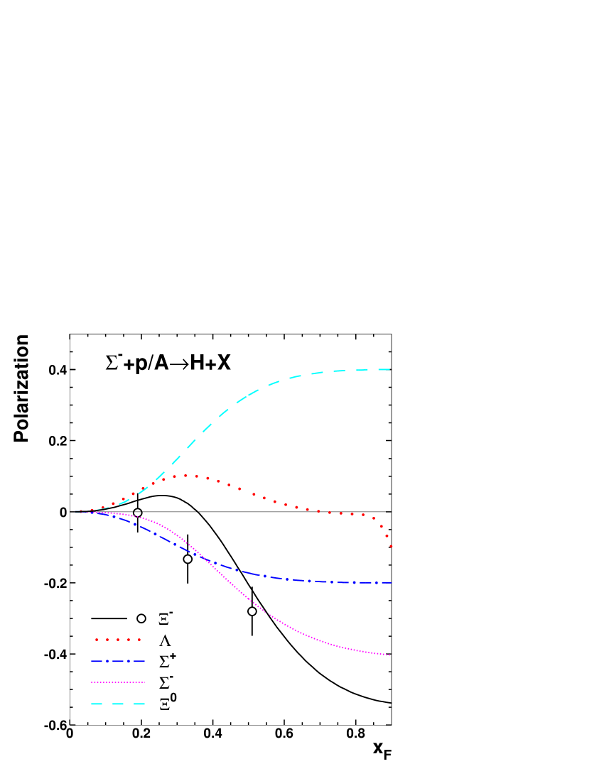
Figure 7: Calculated results for the polarizations of $\Lambda$, $\Sigma^{\pm}$ and $\Xi^{0,-}$ as functions of $x_{F}$. The thin dotted curve represents the polarization of $\Lambda$. Data for $\Xi^{-}$ are taken from Ref. WA89-95 .

- (1) A. Lesnik et al., Phys. Rev. Lett. 35, 770 (1975).
- (2) G. Bunce et al., Phys. Rev. Lett. 36, 1113 (1976).
- (3) For a review of the data, see, e.g., K. Heller, in Proceedings of the 12th International Symposium on High Energy Spin Physics, 1996, Amsterdam, Netherlands, edited by C.W. de Jager, T.J. Ketel, P.J. Mulders, J.E.J. Oberski, and M. Oskam-Tamboezer (World Scientific, Singapore, 1997), p. 23; and the references given there.
- (4) B. Andersson, G. Gustafson and G. Ingelman, Phys. Lett. 85B, 417 (1979).
- (5) T.A. DeGrand and H.I. Miettinen, Phys. Rev. D 24, 2419 (1981).
- (6) J. Szwed, Phys. Lett. 105B, 403 (1981).
- (7) L.G. Pondrom, Phys. Rep. 122, 57 (1985).
- (8) R. Barni, G. Preparata and P.G. Ratcliffe, Phys. Lett. B 296, 251 (1992).
- (9) J. Soffer and N.A. Törnqvist, Phys. Rev. Lett. 68, 907 (1992).
- (10) Liang Zuo-tang, and C. Boros, Phys. Rev. Lett. 79, 3608 (1997).
- (11) Liang Zuo-tang, and C. Boros, Phys. Rev. D 61, 117503 (2000).
- (12) Liang Zuo-tang, and Li Tie-shi, J. Phys. G 26, L111 (2000).
- (13) M. Anselmino, D. Boer, U. D’Alesio, and F. Murgia, Phys. Rev. D 63, 054029 (2001).
- (14) A summary of the data can be found in, e.g., A. Bravar, in Proceedings of the 13th International Symposium on High Energy Spin Physics, Protvino, Russia, edited by N.E. Tyurin et al. (World Scientific ,Singapore, 1999), p. 167; see in particular also Ref. E704 listed below.
- (15) FNAL E704 Collaboration, D.L. Adams et al., Phys. Lett. B 264, 462 (1991); B 276, 531 (1992); Z. Phys. C 56,181 (1992). A.Bravar et al., Phys. Rev. Lett. 75, 3073 (1995); 77, 2626 (1996); D.L. Adams et al., Nucl. Phys. B510, 3 (1998).
- (16) Liang Zuo-tang, and Xu Qing-hua, Phys. Rev. D 65, 113012 (2002).
- (17) R608 Collaboration, T. Henkes, Phys. Lett. B 283, 155 (1992).
- (18) CLAS Collaboration, D.S. Carman et al., Phys. Rev. Lett. 90, 131804 (2003).
- (19) C. Boros and Liang Zuo-tang, Phys. Rev. D 57, 4491 (1998).
- (20) G. Gustafson and J. Häkkinen, Phys. Lett. B 303, 350 (1993).
- (21) ALEPH Collaboration, D. Buskulic et al., Phys. Lett. B 374, 319 (1996).
- (22) OPAL Collaboration, K. Ackerstaff et al., Eur. Phys. J. C 2, 49 (1998).
- (23) Liu Chun-xiu, and Liang Zuo-tang, Phys. Rev. D 62, 094001 (2000); Liu Chun-xiu, Xu Qing-hua and Liang Zuo-tang, ibid. 64, 073004 (2001); Xu Qing-hua, Liu Chun-xiu, and Liang Zuo-tang, ibid. 65, 114008 (2002); Liang Zuo-tang, and Liu Chun-xiu, ibid. 66, 057302 (2002).
- (24) NOMAD Collaboration, P. Astier et al., Nucl. Phys. B588, 3 (2000).
- (25) Xu Qing-hua, and Liang Zuo-tang, Phys. Rev. D 68, 034023 (2003).
- (26) P. Chliapnikov et al., Nucl. Phys. B37, 336 (1972); I.V. Ajinenko et al., Z. Phys. C 5, 177 (1980); K. Paler et al., Nucl. Phys. B96, 1 (1975); Yu. Arestov et al., Z. Phys. C 6, 101 (1980).
- (27) M. Barth et al., Nucl. Phys. B223, 296 (1983).
- (28) EXCHARM Collaboration, A. N. Aleev et al., Phys. Lett. B 485, 334 (2000).
- (29) ALEPH Collaboration, D. Buskulic et al., Z. Phys. C 69, 393 (1995).
- (30) DELPHI Collaboration, P. Abreu et al., Z. Phys. C 68, 353 (1995); Phys. Lett. B 406, 271(1997);
- (31) OPAL Collaboration, K. Ackerstaff et al., Phys. Lett. B 412, 210 (1997); Z. Phys. C 74, 437 (1997); G. Abbiendi et al., Eur. Phys. J. C 16, 61 (2000).
- (32) Xu Qing-hua, Liu Chun-xiu, and Liang Zuo-tang, Phys. Rev. D 63, 111301 (2001).
- (33) C. Boros, Liang Zuo-tang and Meng Ta-chung, Phys. Rev. Lett. 70, 1751 (1993); Liang Zuo-tang and Meng Ta-chung, Phys. Rev. D 49, 3759 (1994).
- (34) C. Boros and Liang Zuo-tang, Phys. Rev. D 53, R2279 (1996).
- (35) Liang Zuo-tang, and C. Boros, Inter. J. Mod. Phys. A 15, 927 (2000).
- (36) Dong Hui, and Liang Zuo-tang, in preparation.
- (37) W. Ochs, Nucl. Phys. B118, 397 (1977).
- (38) W. Kittel, in Partons in Soft-Hadronic Processes, Proceedings of the Europhysics Study Conference, Erice, Italy, 1981, edited by R.T. Van de Walle, (World Scientific ,Singapore, 1981), p. 1.
- (39) K.P. Das and R.C. Hwa, Phys. Lett. 68B, 459 (1977).
- (40) E925 Collaboration, C.E. Allgower et al., Phys. Rev. D 65, 092008 (2002).
- (41) Dong Hui, Li Fang-zhen, and Liang Zuo-tang, Phys. Rev. D 69, 017501 (2004).
- (42) R. Gatto, Phys. Rev. 109, 610 (1958).
- (43) Particle Data Group, K. Hagiwara, Phys. Rev. D 66, 010001 (2002).
- (44) In practise, since there is no data directly on , we determine the two ’s by fitting a few data points at large of the available data on the invariant cress section at a given because apparently . This implies that, we multiply the number densities , and ’s with and a constant which changes the differential cross sections to the number densities. In this way, all of them are changed to their counterparts in the invariant cross section . It is expected that, if the direct fusion model works, should neither strongly depend on nor on . The and dependences of the number density of the hadron produced from this process come predominately from the quarks and/or antiquarks in the initial states. So we can approximately fix the parameters entering a integrated density from data at fixed . For GeV/, the corresponding result for is mb/GeV2, that for is mb/GeV2, and that for is mb/GeV2, For more details, see Refs. BLM93 ; BL96 ; LB00rev given above.
- (45) See, e.g., J.J. Dugne and P. Tavernier Z. Phys. C 59, 333 (1993).
- (46) See, e.g., M. Glück, E. Reya, and A. Vogt, Eur. Phys. J. C 5, 461 (1998).
- (47) See, e.g., M. Glück, E. Reya and A. Vogt, Z. Phys. C 53, 651 (1992).
- (48) A.M. Smith et al., Phys. Lett. B 185, 209 (1987).
- (49) B. Lundberg et al., Phys. Rev. D 40, 3557 (1989).
- (50) E.J. Ramberg et al., Phys. Lett. B 338, 403 (1994).
- (51) C. Wilkinson et al., Phys. Rev. Lett. 58, 855 (1987).
- (52) L. Deck et al., Phys. Rev. D 28, 1 (1983).
- (53) R. Rameika et al., Phys. Rev. D 33, 3172 (1986).
- (54) K. Heller et al., Phys. Rev. Lett. 51, 2025 (1983).
- (55) A. Morelos et al., Phys. Rev. D 52, 3777 (1995).
- (56) J. Duryea et al., Phys. Rev. Lett. 67, 1193 (1991).
- (57) S. A. Gourlay et al., Phys. Rev. Lett. 56, 2244 (1986).
- (58) M. L. Faccini-Turluer et al., Z. Phys. C 1, 19 (1979).
- (59) H. Grassler et al., Nucl. Phys. B136, 386 (1978).
- (60) H. Abramowicz et al., Nucl. Phys. B105, 222 (1976).
- (61) M. Baubillier et al., Nucl. Phys. B148, 18 (1979).
- (62) S. N. Ganguli et al., Nucl. Phys. B128, 408 (1977).
- (63) J. Bensinger et al., Nucl. Phys. B252, 561 (1985).
- (64) B. Adeva et al., Z. Phys. C 26, 359 (1984).
- (65) D. H. Stuntebeck et al., Phys. Rev. D 9, 608 (1974).
- (66) WA89 Collaboration, M. I. Adamovich et al., Z. Phys. A 350, 379 (1995).