A Non-Extensive Model for Quark Matter Produced in Heavy Ion Collisions

Abstract

We describe quark matter in the framework of non-extensive thermodynamics. We point out that particle spectra with power-law tail lead to an increased energy and entropy per particle, and therefore even a massless plasma may fit both the relatively high value of E/N = 1 GeV and the spectral slope of T = 175 MeV observed in RHIC experiments.

I Introduction

The probably most important motivation for relativistic heavy-ion experiments at large scale accelerator facilities (RHIC, SPS) is to study quark matter in a unique environment, possibly in form of a quark-gluon plasma (QGP) produced for a short while before hadronization RHICpt . While the original idea of quark-gluon plasma sticks to an equilibrium picture both in its early, bag-model inspired versions BAGMODEL and in the theoretically most advanced lattice gauge models lattQCD1 ; lattQCD2 , phenomenological studies of the experimental spectra offer an increasing amount of evidence that this equilibrium is not completely achieved CHEMISTRY ; ALCOR ; PARTONS .

In particular the equilibrium thermodynamics relies on (in the Boltzmann limit) exponential particle spectra, while experiments definitely show a power-law tail at high transverse momenta. This means that some assumption leading to the Boltzmann-Gibbs factor is not fulfilled. We have therefore to look for a theoretical description which is more general, which releases one or more original assumptions. Such a candidate is the non-extensive thermodynamics, promoted by Tsallis and others, which is based on an altered definition of the Boltzmann entropy Tsallis1 ; Tsallis2 ; Tsallis3 ; Plastinos ; Tsallis4 ; Tsallis5 . More recently it has been shown that the power-law distribution also can be described by a logarithmic dispersion relation for the quasi-particle energy while keeping the original, extensive entropy definition QWang1 ; QWang2 . In this case the energy is non-extensive. The relevance of Tsallis statistics to high-energy $e^{+}e^{-}$ and heavy-ion collisions has been studied in several papers RELEV . In this paper we show that such a version of non-extensive thermodynamics is able to describe a power-law distribution of quasi-particle energies and explain an apparent spectral temperature, $T=175$ MeV at low energy. Furthermore, the very power in the tail of this distribution can be connected to the energy per particle, $E/N=1$ GeV, which remained unexplained in traditional thermal models.

There were several attempts to describe dynamical mechanisms which would simulate (totally or just in part) a Gibbs distribution or a Tsallis distribution with a power-law tail asymptotics BiMu2004 ; OtherMech1 ; OtherMech2 ; OtherMech3 ; OtherMech4 . Tsallis advocates the non-extensive thermodynamics based on his entropy definition for a general use for systems in non-ergodic states showing exponentially not suppressed distribution tails ExplainTs1 ; ExplainTs2 . Due to this an interesting question arises for the heavy ion physics: can the quark-gluon plasma (QGP) be described in terms of the non-extensive thermodynamics? Would it give a quantitatively better description of experimental observation than the old bag-model picture while being almost as simple? In this paper we shall answer these questions positively by showing that a simple QGP with power-law energy distribution instead of the Gibbs one and a bag constant is able to reach the hadronically fitted temperature of $T_{0}\approx 175$ MeV and the 1 GeV energy per particle at the same time. We extend this study for finite chemical potential using relativistic Fermi and Bose distributions derived according to the rules of non-extensive thermodynamics. After briefly discussing the recently considered directions in this research of extending thermodynamics, we choose the interpretation of Q. Wang QWang1 ; QWang2 , who has revealed that an anomalous (logarithmic) quasi-particle dispersion relation may lie in the background of the canonical Tsallis distribution with the famous power-law tail. We shall study the equation of state (eos) of this QGP and eventually obtain a constant energy per particle curve on the $T-\mu$ plane.

II QGP in non-extensive thermodynamics

The starting point of our description of a quark-gluon matter at the instant of hadronization is based on a power-law energy distribution of partons,

$$w_{1}(E)=(1+E/b)^{-c},$$ (1)

containing two parameters; an energy scale $b$ in the order of 1 to a few GeV and the power $c$, which is expected to be rather high, 4-10, extracted from fits to minijet distribution in a pQCD based theoretical parton dynamics model FriesNonaka ; Fries . The ZEUS collaboration extracted the value $c=5.8\pm 0.5$ in $e^{+}e^{-}$ experiments ZEUS . In the double limit, $c\rightarrow\infty$, $b\rightarrow\infty$ with a fixed ratio $T=b/c$ this distribution approaches the familiar canonical Gibbs-Boltzmann formula,

$$w_{\infty}(E)=\exp(-E/T).$$ (2)

As it has been indicated in Ref.BiMu2004 parton recombination, which is most likely to happen at low relative energies and therefore combines a parton cluster or pre-hadron with energy $E$ from two partons with energy $E/2$, or in general from $n$ partons each with an energy of $E/n$, drives the power-law distribution towards the exponential limit:

$$w_{n}(E)=(1+E/(nb))^{-nc},$$ (3)

by increasing both the effective $c$ and $b$ to $nc$ and $nb$ while keeping their ratio $T=nb/nc=b/c$ constant. The power-law distribution we are using here is related to a canonical Tsallis distribution by setting the temperature $T=b/c$ and the Tsallis index to $q=1+1/c$ when considering $w^{q}$-weighted averages of energy and particle number as thermodynamical observables. Funny enough, using the ”normal”, $w$-weighted averages as macroscopic variables one arrives at $q=1-1/c$.

An anomalous thermodynamics based on an altered definition of the entropy,

$$S=\frac{1}{1-q}\sum_{i}(w_{i}^{q}-w_{i}),$$ (4)

has been worked out by Tsallis and several other authors Tsallis1 ; Tsallis2 ; Tsallis3 ; Plastinos ; Tsallis4 ; Tsallis5 . It resembles the Legendre transformation structure and herewith the canonical and grand canonical versions of phase space distributions behind observable macroscopic expectation values. The distribution (1) can be viewed as the canonical Tsallis distribution

$$w_{i}=\frac{1}{Z}\left(1+\frac{(q-1)E_{i}}{T}\right)^{\frac{1}{1-q}}$$ (5)

with the canonical partition function,

$$Z=\sum_{i}\left(1+\frac{(q-1)E_{i}}{T}\right)^{\frac{1}{1-q}}.$$ (6)

The interpretation of the temperature $T$ and the Tsallis-index $q$ (related to the power-low cutoff $b$ and power $c$) is still subject to the fact, however, that which version of macroscopic observables are considered in the effective, ”non-extensive” thermodynamics. By now the choice

$$E=\sum_{i}w_{i}^{q}E_{i}/\sum_{i}w_{i}^{q},$$ (7)

and the canonical variational principle,

$$S-\beta E={\rm max.}$$ (8)

seem to establish themselves. (However, a recent article QWang2 righteously criticizes this choice. According to the interpretation given there the ”normal” macroscopic averages are meaningful as well.) In the grand-canonical version $E$ is replaced by $X=E-\mu N$, and $E_{i}$ by $X_{i}=E_{i}-\mu Q_{i}$. The expression to be minimized becomes $S-\beta X$.

In the following we review the most important details of these calculations. Considering the derivatives with respect to $w_{i}$,

$$\frac{\partial}{\partial w_{i}}S = c(1-qw_{i}^{1/c}),$$

$$\frac{\partial}{\partial w_{i}}X = q\frac{w_{i}^{1/c}}{\sum w_{j}^{q}}(X_{i}-X),$$ (9)

one arrives at the constraint

$$1=\left(1+\beta\frac{X_{i}-X}{c\sum w_{j}^{q}}\right)qw_{i}^{1/c}$$ (10)

This gives rise to a grand-canonical distribution $w_{i}$ proportional to a $(-c)$-th power:

$$w_{i}\propto\left(1+\beta\frac{X_{i}-X}{c\sum w_{j}^{q}}\right)^{-c}.$$ (11)

This can be casted into the Tsallis form,

$$w_{i}=\frac{1}{Z}\left(1+\frac{X_{i}}{cT}\right)^{-c}$$ (12)

normalized by the partition sum,

$$Z=\sum_{i}\left(1+\frac{X_{i}}{cT}\right)^{-c}.$$ (13)

The temperature, $T$ is, however, no more related to the Lagrange multiplier $\beta=1/\Theta$ as straight as usual. It is

$$T=\Theta\sum w_{j}^{q}-X/c.$$ (14)

Since the original probability is normalized,

$$\sum_{i}w_{i}=1,$$ (15)

in general $\sum_{i}w_{i}^{q}$ differs from one.

In order to make the discussion more transparent we use the following abbreviations for the high-power-law distribution function and its inverse:

$$\exp_{c}(x) =(1-x/c)^{-c} \longrightarrow\exp(x),$$

$$\ln_{c}(x) =c(1-x^{-1/c}) \longrightarrow\ln(x).$$ (16)

The limits are valid for $c\rightarrow\infty$ by fixed $T=b/c$. These functions are inverse to each other, $\exp_{c}(\ln_{c}(x))=x$, and reflect the non-extensive property,

$$\ln_{c}(xy)=\ln_{c}(x)+\ln_{c}(y)-\frac{1}{c}\ln_{c}(c)\ln_{c}(y).$$ (17)

The derivatives of these functions follow rules similar to the familiar ones:

$$\frac{d}{dx}\exp_{c}(x) = \exp_{c}^{q}(x),$$

$$\frac{d}{dx}\ln_{c}(x) = 1/x^{q}.$$ (18)

The Tsallis entropy with this notation reads as

$$S=\sum_{i}w_{i}\ln_{c}(1/w_{i}),$$ (19)

and in case of equiprobability, $w_{i}=1/N$ for $N$ states, one arrives at

$$S=\ln_{c}(N),\qquad{\rm and}\qquad N=\exp_{c}(S).$$ (20)

The grand-canonical distribution and partition sum becomes

$$w_{i}=\frac{1}{Z}\exp_{c}(-X_{i}/T),\qquad Z=\sum_{i}\exp_{c}(-X_{i}/T).$$ (21)

The anomalous thermodynamics reflects familiar looking relations, with some exceptional points. The heat is expressed by

$$\Theta S\sum_{i}w_{i}^{q}\,=\,T\ln_{c}Z+E-\mu N,$$ (22)

with the grand canonical partition sum

$$Z=\sum_{i}\exp_{c}(-(E_{i}-\mu Q_{i})/T),$$ (23)

where we use the q-weighted particle number,

$$N=\sum_{i}w_{i}^{q}Q_{i}/\sum_{i}w_{i}^{q},$$ (24)

and the chemical potential, $\mu$, the corresponding Lagrange multiplier. Here $Q_{i}$ are the conserved charges of the state $i$. The pressure, assuming homogeneity in a sufficiently large volume, $V$, is given by

$$p=\frac{T}{V}\ln_{c}Z.$$ (25)

Resolving expression (14) for $\Theta$ one arrives at the following grand canonical potential

$$-\Omega=pV=T\ln_{c}Z=TS-(E-\mu N)(1-S/c).$$ (26)

The derivatives are given by

$$\frac{\partial}{\partial V}\Omega=-p,\qquad\frac{\partial}{\partial T}\Omega=-S,\qquad\frac{\partial}{\partial\mu}\Omega=-N(1-S/c).$$ (27)

For the energy per particle the correction factor $(1-S/c)$, by chance, does not play a direct role:

$$E/N\,=\,\frac{\mu(\partial p/\partial\mu)+T(\partial p/\partial T)-p}{\partial p/\partial\mu}.$$ (28)

In case of an ideal (but still power-law, not Gibbs-distributed) gas one assumes that

$$p(\mu,T)=\int\!\frac{d^{3}k}{(2\pi)^{3}}\,T\ln_{c}Z$$ (29)

with

$$Z=\sum_{n}\exp_{c}(-nx),$$ (30)

and

$$x_{k}=E_{k}-\mu Q_{k}.$$ (31)

(Here $Q_{k}=Q$, the conserved charge is usually independent of the momentum of the considered particle.) For fermions the summation runs over $n=0$ and $n=1$ only, while for bosons for all positive integers $n=0,1,2,\ldots$. In this paper we shall deal with massless relativistic particles (quarks and gluons), so practically $E_{k}=|\vec{k}|.$ The derivative relations known for the ordinary ideal gas are almost fulfilled,

$$n=\frac{\partial p}{\partial\mu},\qquad s=\frac{\partial p}{\partial T},\qquad e=\mu n+{\Theta}s-p$$ (32)

for the particle-, entropy- and energy-density, respectively.

Constructing this way the Tsallis-Bose and Tsallis-Fermi distributions (alternative ways can be found in BEetFDinTS ), one may use the following integral representation of the power-law function:

$$\exp_{c}(-x)=\frac{1}{\Gamma(c)}\int_{0}^{\infty}\!dt\,t^{c-1}\>e^{-t(1+x/c)}$$ (33)

where $\Gamma(c)$ is Euler’s Gamma function giving $(c-1)!$ for integer $c>1$. This representation relates the grand canonical partition function $Z$ of anomalous thermodynamics to the usual one-particle forms of Fermi and Bose distributions, respectively:

$$Z=\frac{\int_{0}^{\infty}\!dt\,t^{c-1}e^{-t}\zeta(tx/c)}{\int_{0}^{\infty}\!dt\,t^{c-1}e^{-t}},$$ (34)

where $\zeta(y)=1+\exp(-y)$ for the Fermi, and $\zeta(y)=1/(1-\exp(-y))$ for the Bose distribution. This form is quite suggestive: the Tsallis thermodynamics is an average of ”normal” systems with an Euler-Gamma distributed parameter, factorizing the energy. Applying it for $x=E/T$ we substitute $y=tE/b$, the scaled energy into the ”normal” partition function $\zeta$. This sheds some light on interpretations of Tsallis-distributed particle spectra in terms of a temperature fluctuating according to the Gamma distribution OtherMech3 or energy non-conservation due to higher than two-body collisions, again with Gamma distributed energy imbalance RAFLET ; BOLeqinTS . These correspondences are, of course, no explanations for the power-law distribution, but rather equivalent re-formulations, assuming the Gamma distribution for the corresponding (Legendre associated) intensive variable.

Our main goal in this paper is to investigate the original idea of quark-gluon plasma in terms of the anomalous, non-extensive thermodynamics. Therefore we do not wish to speculate here about the microscopic dynamical mechanisms, which lead to the power-law distribution, closely approximating exponential spectra in the intermediate transverse momentum range. We assume now, that an anomalous QGP of massless and Tsallis distributed particles have existed before hadronization and ask the question whether this state is realistic, whether it is nearer or farer from the state of hadronic matter observed in RHIC (and partially in SPS) experiments with many of its properties surprisingly well fitted by traditional equilibrium thermodynamical concepts underlying the hadronic thermal model ThMOD1 ; ThMOD2 ; ThMOD3 ; ThMOD4 . For this purpose we select the energy per particle $E/N$ as a decisive observable; it can be quite directly measured on the one hand and quite easily calculated in thermodynamical framework on the other hand. Considering a bag constant also in the case of Tsallis QGP, we shall modify $E/N$ accordingly. Another interesting quantity is the entropy per particle, $S/N$. It can be related to other thermodynamical quantities as

$$\frac{S}{N}=\frac{s}{n}=\frac{e+p}{nT}-\frac{\mu}{T}.$$ (35)

III Energy per particle

For calculating $E/N$ it is helpful to introduce notations for the $(1-S/c)$ uncorrected derivatives of the pressure, $e_{0}=T\partial p/\partial T+\mu\partial p/\partial\mu-p$, and $n_{0}=\partial p/\partial\mu$. Since the derivatives of the pressure with respect to $T$ and $\mu$ can be regarded as derivatives of $\ln_{c}Z(x)$ with respect to $x$ under the phase space integral by noting that $\partial/\partial x$ acts as $-T\partial/\partial E_{k}$ or $T\partial/\partial\mu$ respectively, we get

$$n_{0} = \int\!\frac{d^{3}k}{(2\pi)^{3}}\,f_{c}({\frac{E_{k}-\mu}{T}}),$$

$$e_{0} = \int\!\frac{d^{3}k}{(2\pi)^{3}}\,E_{k}f_{c}({\frac{E_{k}-\mu}{T}}),$$ (36)

with the one-particle distribution function

$$f_{c}(x)=-\frac{\partial}{\partial x}\ln_{c}Z(x).$$ (37)

Now we have simply $E/N=e_{0}/n_{0}$.

Before dealing with Fermi and Bose statistics in the anomalous thermodynamics let us first review the dilute matter limit, the Tsallis-Boltzmann approximation. This relies on the assumption that $\exp_{c}(-x)\ll 1$. Now $Z=1$ to leading order and there is no difference between Fermi and Bose distributions,

$$f_{c}(x)\approx-\frac{d}{dx}\ln_{c}(1+\exp_{c}(-x))\approx-\frac{d}{dx}\exp_{c}(-x)=\left(1+\frac{x}{c}\right)^{-c-1}.$$ (38)

A (slight) difference can be observed between the inverse slope of logarithmic one-particle spectra and the temperature,

$$(c+1)T_{{\rm slope}}=cT=b.$$ (39)

We carry out our first estimate at $\mu=0$ and finite temperature in the Boltzmann approximation. Using $f_{c}(E)=(1+E/b)^{-c-1}$ in the corresponding integrals (36), we get

$$n_{0} = \frac{d}{2\pi^{2}}\frac{2b^{3}}{c(c-1)(c-2)},$$

$$e_{0} = \frac{d}{2\pi^{2}}\frac{6b^{4}}{c(c-1)(c-2)(c-3)},$$ (40)

with a common (color, spin, etc.) degeneracy factor $d$. In the low energy region we obtain a simple relation between the energy per particle and the inverse slope of the one-particle spectra,

$$E/N=e_{0}/n_{0}=\frac{c}{c-3}3T=\frac{3(c+1)}{(c-3)}T_{{\rm slope}}.$$ (41)

This differs from the familiar relation, $E/N=3T$, known for the massless Boltzmann gas. It is interesting to note, that – as it has been calculated in Ref.Lavagno1 ; Lavagno2 – by using the normal weighted definition for particle number, $N^{\prime}=\sum_{i}w_{i}Q_{i}$, one gets $E/N^{\prime}=3T$. We do not think, however, that using different definitions for the macroscopic energy and particle number would make a sense in comparison with experimental data: either $w_{i}$ or $w_{i}^{q}$ is the distribution of physical states. Furthermore $T$ is not exactly the ”experimental temperature” conjectured from the inverse spectral slope.

An estimate of the inverse slope gives rise to $T_{{\rm slope}}\approx 175$ MeV for RHIC experiments in the $\mu\approx 0$ region. This is also the value used by conventional thermal models for the temperature. Aiming at $E/N=1$ GeV now, the formula (41) leads to a power of $c+1\approx 8.42$ in the one-particle distribution $f_{c}(E)$, a value comparable with minijet $p_{T}$-distribution fits Fries ; FriesNonaka . Neither the traditional Boltzmann formula, $E/N=3T$, nor the simple bag model of QGP, where $E/N=4T$, is able to describe both this inverse slope and energy per particle at the same time.

In order to display a more throughout comparison to the thermal model points in the $T-\mu$ plane fitted to different accelerator experiments StachREVIEWS , we carried out numerical integrations with Tsallis-Fermi and Tsallis-Bose distributed, massless quark-gluon plasma at finite temperature and chemical potential. In this case, denoting a general integral of $f_{c}(x)$ weighted with a power $x^{n}$ by

$$I_{n}(a)=\int_{-a}^{\infty}dx\,x^{n}\,f_{c}(x),$$ (42)

and the symmetric and anti-symmetric combinations, $S_{n}(a)=I_{n}(a)+I_{n}(-a),$ $A_{n}(a)=I_{n}(a)-I_{n}(-a)$, we arrive at

$$2\pi^{2}\>n_{0} = T^{3}S_{2}(\mu/T)+2T^{2}\mu A_{1}(\mu/T)+T\mu^{2}S_{0}(\mu/T),$$

$$2\pi^{2}\>e_{0} = T^{4}S_{3}(\mu/T)+3T^{3}\mu A_{2}(\mu/T)+3T^{2}\mu^{2}S_{1}(\mu/T)+T\mu^{3}A_{0}(\mu/T),$$ (43)

for each fermion. For the boson part we assume $\mu=0$. The energy per particle characteristic for the power-law distributed mixture then becomes

$$E/N=\frac{d_{B}e_{0B}(T)+d_{F}e_{0F}(T,\mu)+d_{F}e_{0AF}(T,\mu)}{d_{B}n_{0B}(T)+d_{F}n_{0F}(T,\mu)+d_{F}n_{0AF}(T,\mu)}.$$ (44)

Before presenting our numerical results there is one more aspect of this version of the anomalous thermodynamics to be discussed. In the traditional, Gibbs thermodynamics the anti-fermion distribution is related to the fermion distribution simply by a change in the sign of the baryochemical potential, $\mu$. This formula exactly coincides with the density of fermion holes:

$$1-f_{\infty}((-E-\mu)/T)=f_{\infty}((E+\mu)/T)$$ (45)

due to $f_{\infty}(x)+f_{\infty}(-x)=1$ for the Fermi distribution $f_{\infty}(x)=1/(1+\exp(x))$. This relation is not fulfilled for a finite $c$ index Tsallis-Fermi distribution:

$$f_{c}(x)=(1+\exp_{-c}(x))^{-q}.$$ (46)

In this case

$$f_{c}((-E-\mu)/T)+f_{c}((E+\mu)/T)=f_{c}(-x)+f_{c}(x)\neq 1,$$ (47)

instead

$$f_{c}^{1/q}(x)+f_{-c}^{1/q}(-x)=1$$ (48)

is fulfilled. Here the anti-charge choice with $-\mu$ and the particle hole choice by replacing $-E$ energy are not equivalent. For the estimate of the energy per particle of a Tsallis QGP at finite temperature $T$ and baryochemical potential $\mu$ in Ref.RHIC-SCHOOL we utilized the particle-hole correspondence:

$$\overline{f}_{c}(E;\mu,T)=1-f_{c}(-E;\mu,T).$$ (49)

Now we turn to another interpretation of the non-extensive thermodynamics, similar to that suggested by Q. Wang QWang1 ; QWang2 ; EXTversionTS , which handles the fermions and antifermions in a more satisfactory manner.

IV Quasiparticles and anomalous thermodynamics

In the preceding discussion we have already indicated some disadvantages of the ”main stream” Tsallis formulation of non-extensive thermodynamics. These make it to be not the best choice for our purpose, i.e. for using it in the description of quark matter. The dependence of some thermodynamical relations indirectly on the system size (i.e. dependence of densities on the total entropy, etc.), the slight difference between temperature parameter and one-particle distribution inverse slope, and finally the strange correspondence between particles and holes in the Fermi distribution leave us with dissatisfaction. Also the very basic point, the non-extensivity of the Tsallis-entropy remains a challenge for the physical interpretation (and acceptance) of this approach.

Fortunately it has been shown meanwhile that a mathematically well-defined monotonous function of the Tsallis entropy describes an extensive entropy measure Abe ; QWang1 . The Tsallis-entropy satisfies the general rule of pseudo-additivity,

$$f(S_{12})=f(S_{1})+f(S_{2})+\lambda f(S_{1})f(S_{2}),$$ (50)

required by the existence of thermal equilibrium in non-extensive composite systems. The Tsallis-entropy realizes the case $f(S)=S$ and $\lambda=1/c=q-1$. The additive, i.e. extensive measure of entropy then becomes

$$\tilde{S}\,=\,\frac{1}{\lambda}\>\ln(1+\lambda f(S)).$$ (51)

Based on the maximalization of $\tilde{S}$ of the Tsallis-entropy instead of $S$ itself, a formally traditional thermodynamics and canonical, or grand canonical distribution emerges QWang2 . The price to pay for that is, that the energy (and incidentally the particle number and the volume) is no more an extensive quantity. It is a clear indication that the Tsallis entropy describes systems whose parts still interact with long range forces. The Tsallis canonical distribution and partition sum can be transformed into an ordinary canonical partition sum using a ”deformed Hamiltonian”. By defining

$$\tilde{H}=\frac{1}{\beta(q-1)}\ln\left(1+(1-q)\beta(H-\mu N)\right)$$ (52)

one arrives at

$$Z={\rm Tr}\left(1-(q-1)\beta(H-\mu N)\right)^{1/(q-1)}={\rm Tr}e^{-\beta\tilde{H}}.$$ (53)

As a consequence the Fermi and Bose distributions keep their traditional forms as functions of the eigenvalues of the deformed Hamiltonian, $\tilde{H}$. The trace over the states of the many particle system leads to a product over the phase space labels of independent quasi-particles with energy $\omega_{k}$, and the one-particle distribution becomes

$$f(k)=\frac{1}{e^{\omega_{k}/T}\pm 1}=\frac{1}{(1+(E_{k}-\mu)/cT)^{c}\pm 1}.$$ (54)

where $E_{k}$ is the eigenvalue of the original Hamiltonian, i.e. the energy of an interacting quark or gluon with momentum $k$. For particle and nuclear physics purposes this use of a quasi-particle energy is the more enlightening approach.

For the investigation of a long range interacting quark matter we still have to modify the above picture a little. The power-law tail with a general, fractional power restricts the base of this power-law to be positive. In a picture of a QGP rooting in QCD on the other hand gluons are exactly and quarks are practically massless, therefore $E_{k}=|k|$ can be as small as zero. For any finite, positive chemical potential $\mu>0$ the above distribution may become complex, unless $\mu<cT=b$. This restricts the use of quark chemical potentials too seriously. We explore therefore here another approach.

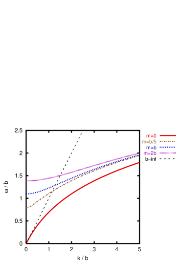
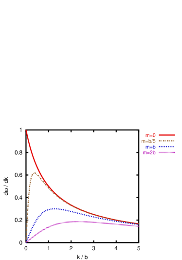
Figure 1: Anomalous dispersion relations and group velocities for Tsallis quark matter.

Repeating the above line of derivation given by Q.Wang we start with the anomalous dispersion relation for the QGP quasi-particles:

$$\omega_{k}=b\ln(1+E_{k}/b)$$ (55)

with $E_{k}=\sqrt{k^{2}+m^{2}}$ being the dispersion relation of a free relativistic particle with mass $m$. Fig.1 shows this for different masses. The right side of the figure plots the group velocity, $v_{g}=d\omega/dk$, which overall remains below one. Such a dispersion relation does not violate causality. Still it is anomalous; it shows an acoustical branch LANDAU ; SOLIDtxtbook for the massless case, and a line crossing from the optical branch at low momenta to an acoustical behavior at high momenta for finite mass. Such a quasi-particle dispersion relation has never been considered yet in QCD, as far as we know QUASI1 ; QUASI2 ; QUASI3 . The plasmons all live on the optical branch, above the light cone. Below the light cone a series of Landau poles can be located, they cannot belong to traditional ”particles”. It is also hard to find a (partial) summation of diagrams leading to a logarithmic dispersion relation from QCD. But the proof of impossibility is also unknown.

The investigation of the non-relativistic and extreme relativistic limit of the formula (55) may help to approach to a physical interpretation. Based on the second derivative,

$$\frac{d^{2}\omega_{k}}{dk^{2}}\,=\,\frac{m^{2}/\omega_{k}+(m^{2}-k^{2})/b}{(\omega_{k}+\omega_{k}^{2}/b)^{2}}$$ (56)

we get in the non-relativistic range $0\ll k\ll m$ (which nevertheless cannot be applied to massless QGP)

$$\omega_{k}=b\log(1+\frac{m}{b})+\frac{b}{b+m}\frac{k^{2}}{2m}+\ldots$$ (57)

This features an attractive mean field effect for the heavy quarks in QGP due to $\omega_{0}<m$, and an increased effective mass $m_{eff}=m(1+m/b)$. For relativistic (including $m=0$) particles the quasi-particle mass cannot be interpreted other than the inverse of the second derivative of the dispersion relation at $k=0$, which is zero as defined above. At any finite $k$ the second derivative is negative, not corresponding to any picture of a traditional point particle.

It is also interesting to interpret this dispersion relation in the framework of plasma physics. In plasmas a dielectric coefficient, $\varepsilon(\omega,k)$, may alter the free dispersion relation. The pole of the propagator in medium is located at

$$D^{-1}=\omega^{2}-k^{2}/\varepsilon=0.$$ (58)

From this we get

$$\sqrt{\varepsilon}=\frac{k}{\omega_{k}}=\frac{k/b}{\ln(1+k/b)}$$ (59)

which is greater or equal to one. This is a further anomalous property, related to a negative self-energy (due to $D^{-1}=\omega^{2}-k^{2}-\Pi$, $\Pi=k^{2}(1/\varepsilon-1)$ ). This property also occurs in non-abelian gauge theories, where gluon loop contributions render the gluon self energy negative. This effect is alike asymptotic freedom, a vanishing charge at high momenta. Classically $\alpha=\alpha_{0}/\varepsilon$, according to eq.(59) this quantity tends to zero at $k\rightarrow\infty$. The very functional form of this running coupling, however, differs from the usual 1/log one, known from perturbative QCD.

The one-particle distribution functions (Fermi and Bose) in the Boltzmann approximation become simple power-laws:

$$f(k)=\exp(-(\omega_{k}-\mu)/T)=\exp(\mu/T)\left(1+\frac{E_{k}}{b}\right)^{-b/T}$$ (60)

with a power $c=b/T$. Now the chemical potential $\mu$ does not enter under a logarithm, which makes it possible to obtain real results at any value of it. The Fermi and Bose distribution becomes

$$f(k)=\frac{1}{\exp{(\omega_{k}-\mu)/T}\pm 1}=\frac{1}{\exp(-\mu/T)\left(1+E_{k}/b\right)^{c}\pm 1}.$$ (61)

In the $c\rightarrow\infty$ limit the equilibrium thermodynamics of an ideal gas is re-established. Otherwise a power-law tail occurs for momenta around and higher than $b$. Fig.2 shows these distributions for the value $b=1.0325$ GeV, favored by the RHIC experiment slope $T=175$ MeV and an energy per particle of $E/N=1$ GeV.

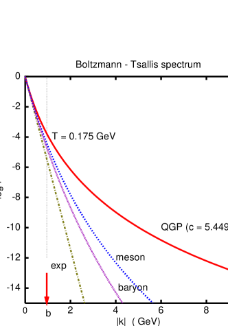
Figure 2: One-particle distributions in Tsallis-QGP. Quarks or gluons correspond to $c=5.4496$, mesons to $2c$ and baryons to $3c$ according to the recombination idea. An exponential fit to $k=0$ is also indicated.

This anomalous behavior can be traced back to one feature: the familiar exponential equilibrium distribution has been modified at high momenta. This contradicts to the traditional result from perturbative QCD, so it cannot stem from an interaction correction to the static, equilibrium state at finite temperature. We rather think it may be related to a characteristically short time scale preventing equilibrium. The short-time behavior is somehow non-particle like, probably related to high off-shell-ness of emerging hadrons.

Recovering the power-law in the Tsallis-Boltzmann approximation, the important thermodynamical quantities coincide with our previous results [ref RHIC]. An other important limit, the $T=0$ Fermi distribution also can be calculated analytically for massless quark matter using the logarithmic dispersion relation (55). The contributions to pressure, energy density and particle density follow the traditional relation, $e=Ts+\mu n-p.$ Considering a bag constant, $e=e_{0}+B$ and $p=p_{0}-B$ still satisfy this relation. The stability edge line, where $p=0$, can be realized by $p_{0}=B$, and therefore $e=e_{0}+p_{0}$. On this edge of the QGP stability against clustering, – possibly a state at the hadronization process, – the energy per particle and the entropy per particle are linearly related for any ideal quasi-particle system. In particular at $T=0$, $E/N=\mu$ has to be fulfilled. As a consequence a hadronic thermal model with $E/N=1$ GeV would have to end at $\mu_{B}=1$ GeV. This estimate does not leave much room for $\mu=\mu_{B}/3$ massless quarks as immediate precursors of the hadrons at the same energy per particle at $T=0$.

Direct integration under the Fermi energy $\mu$ gives the following results at zero temperature:

$$p_{0} = \langle\frac{k}{3}\frac{d\omega}{dk}\rangle=\frac{b^{4}}{6\pi^{2}}\left(x-\frac{x^{2}}{2}+\frac{x^{3}}{3}-\ln(1+x)\right)$$

$$e_{0} = \langle\omega\rangle=\mu n-p_{0}$$

$$n = \langle 1\rangle=\frac{b^{3}}{2\pi^{2}}\frac{x^{3}}{3}.$$ (62)

with $x=k_{F}/b$. The Fermi momentum can be obtained by inverting the logarithmic dispersion relation, $k_{F}=b(e^{\mu/b}-1)$. Considering baryons made of three quarks, finally we set $\mu_{B}=3\mu$. In the $b\rightarrow\infty$ limit, realizing that the pressure subtracts from the first three terms in the Taylor expansion of $\ln(1+x)$ exactly $\ln(1+x)$, it is easy to see that $p_{0}=\mu^{4}/(24\pi^{2})$. In this small $x$ ($k_{F}\ll b$, dilute, cold quark matter) limit $e_{0}/n\approx b(3x/4+9x^{2}/10+x^{3}/6+\ldots)$, so the pure energy per particle is $e_{0}/n=3\mu/4$.

V Numerical results

Finally we present results of numerical integrations at arbitrary $T$ and $\mu$ with logarithmic dispersion relation for massless quark matter. First, Fig.3 plots the direct energy per particle $e_{0}/n$ as a function of temperature for different chemical potentials, utilizing the $b=1.0325$ GeV value. The requirement of having $E/N=1$ GeV at $\mu=0$ in this case leads to $T=195$ MeV. Alternatively $T=175$ MeV is achieved by the choice of $b=0.8275$ GeV.

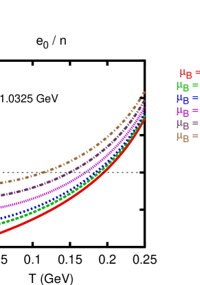
Figure 3: Energy per particle in Tsallis-QGP without a bag constant.

The direct $e_{0}/n=1$ GeV lines on the $T-\mu$ plane are shown in Fig.4.The constant power, $c=4.72732$ line (solid line) approaches the data of the hadronic thermal model (boxes) most closely, however only with the $\mu=\mu_{B}$ assumption. This is not readily a quark matter, where $\mu=\mu_{B}/3$ would be. Massless baryon clusters as prehadrons satisfy rather this assumption, but this idea – however exotic on its own right – does not have yet any support from microscopic models. The constant dispersion relation with $b=0.82728$ GeV plots another line. This deviates even more at $T=0$ from the hadronic boxes, contrary to the fit to the same point at $\mu=0$. (Both the $c$ and the $b$ value were obtained from $E/N=1$ GeV at $\mu=0$ and $T=0.175$ GeV.) Finally the traditional, massless ideal gas corresponding to the exponential spectra ($c=\infty$) are vastly off from the experimental data.

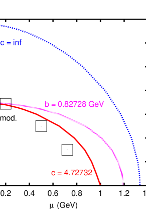
Figure 4: The 1 GeV energy per particle line without bag constant in the $T-\mu$ plane. The constant power, $c=4.72732$, line is solid, the constant energy parameter, $b=0.82728$ GeV line is dashed-dotted, the traditional thermal line ($c=\infty$) is dotted. Boxes show corresponding values from the hadronic thermal model.

The entropy per particle is a sensitive observable, because cannot decrease in spontaneous hadronization processes unless there are more hadrons than quarks and gluons before. It is plotted in the massless ideal Tsallis-gas scenario along the $E/N=1$ GeV curve as a function of the temperature. The solid line corresponds to a constant $c=4.72732$. It is worth to note that it ends at a finite value at $T=0$, contradicting to the third law of thermodynamics. Probably the $c=$constant assumption is not realistic. (Of course this deviation is proportional to $1/c$ as it is easy to see from a low-$T$ expansion of the Fermi distribution.) The constant $b=0.82728$ GeV curve (dashed-dotted) and the traditional thermodynamics (dashed) curve both start from zero at $T=0$. However, only the finite $b$ case can fit the high value of $S/N\approx 6.7$ at $T=0.175$ GeV dictated by the $E/N=1$ GeV for massless bosons and fermions.

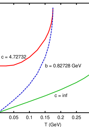
Figure 5: Along the 1 GeV energy per particle line without bag constant in the $T-\mu$ plane the entropy per particle, $S/N$, is plotted. The constant power, $c=4.72732$, line is solid, the constant energy parameter, $b=0.82728$ GeV line is dashed-dotted, the traditional thermal line ($c=\infty$) is dashed.

Taking into account a possible bag constant in Tsallis-QGP with logarithmic ”quasi-particle” energy, the fitted $b$ value becomes $1.0325$ GeV. In Fig.6 the (kinetic + bag) energy per particle, $(e_{0}+p_{0})/n$ at the $p=0$ stability limit is plotted as function of the temperature, $T$ (left part), and as a function of the chemical potential, $\mu_{B}=3\mu$ (right part).

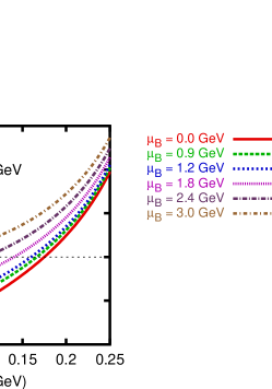
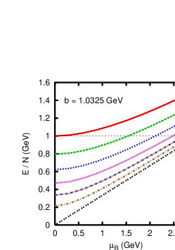
Figure 6: Energy per particle in a Tsallis-QGP with adjusted bag constant to the $p=0$ line. Isochors (left) and isotherms (right) are shown.

Finally we present the $p=0$ stability line for a constant $b=1.0325$ GeV dispersion relation, while adjusting the bag constant $T$ and $\mu$ dependent so, that the total energy per particle, $E/N=(e_{0}+p_{0})/n$ remains constant, $1$ GeV. We find that of all Tsallis-distributed massless QGP models this prescription may come the closest to the hadronic thermal model data. Still the low $\mu_{B}$ value of the hadronic fits to exponential spectra cannot be achieved, pointing out that massless QGP at lower-energy heavy-ion experiments is probably not the state of matter at hadronization, not even with power-law high-momentum tail. Instead massive quarks and gluons have to be considered, which would allow to reach high $E/N$ and $S/N$ values with high-$p_{t}$ powers closer to the experimental values. At RHIC energies, however, this picture is promisingly consistent.

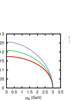
Figure 7: The $E/N=1$ GeV line with $p=0$ adjusted bag constant on the $T-\mu_{B}$ plane ($\mu_{B}=3\mu$ assumed).

VI Conclusion

In conclusion we have worked out the thermal properties of a plasma of massless quarks and gluons utilizing a power-law energy distribution and the Tsallis type anomalous thermodynamic rules. This model describes a non-equilibrium situation or a non-ergodic stationary state: some correlations are not suppressed exponentially, one particle distributions show a long tail in energy and hence in transverse momenta.

This is exactly the case which has been observed in relativistic heavy ion collisions at RHIC at high transverse momenta. The Tsallis QGP is able to offer a temperature and energy per particle value which are near to the ones fitted by hadronic thermal models; a property not shared by traditional quark gluon plasma models. This way a natural precursor state may be suspected at hadronization, as well as an explanation may be given for the value $E/N\approx 1$ GeV. Furthermore we have extended this estimate for finite baryochemical potential using Fermi-Tsallis and Bose-Tsallis statistics for quarks and gluons respectively. Also in this case one can come near to the hadronic thermal model curve with certain power fits, however, due to some indefiniteness in the treatment of anti-fermions the results are less convincing.

A possible solution to this problem is offered by introducing a monotonous re-scaling of Tsallis entropy, which leads to a straightforward correspondence between traditional and Tsallis distributions. The key to this is a logarithmic dispersion relation for the quasi-particles, which has an anomalous character, as we have discussed. This leads to an anomalous thermodynamics, in which now the anti-particles can be interpreted as holes in the particle distribution also for the extended, non-extensive Tsallis distribution. We have repeated the numerical analysis of the energy per particle and the spectra for this case, and realized that the basic qualitative features do not change.

Our final conclusion from these studies is that in order to interpret experimental observations on the bulk particle spectra in relativistic heavy-ion collisions we need to use at last generalized thermodynamical concepts instead of the traditional ones. In particular only this approach allows an interpretation of a spectral slope, a high tail with power-law and the fitted $E/N\approx 1$ GeV energy per particle on the QGP side at the same time.

It remains to clarify what mechanism leads to an anomalous statistics in these heavy ion collisions and to explain the very power. This is a task on its own right, here we just try to sketch some ideas about a possible explanation. Considering non-ergodic, but stationary solution of a Boltzmann equation for partons, special energy dependent cross sections may lead to an approximate validity of simple recombination rules ALCOR ; BialCOALESC ; FriesNonaka . The power-law distribution recombines in this case to distributions closer and closer to the familiar exponential BiMu2004 . Analog to the ”canonical suppression”, which considers effects due to a finite volume on the grand canonical distribution CANSUP ; StachREVIEWS , here we aim to consider finite-time effects leading to partially-equilibrated distributions.

Acknowledgment This work has been supported by the Hungarian National Research Fund, OTKA (T034269). Enlightening discussions with J. Zimányi are gratefully acknowledged.

References

- (1) K. Reygers for the PHENIX Collaboration, nucl-ex/0310010.
- (2) A.Chodos, R.L.Jaffe, K.Johnson, C.B.Thorn, V.Weisskopf,i
- (3) Z. Fodor, S.D. Katz, Phys. Lett. B 534, 87, 2002; Z. Fodor et. al., Nucl. Phys. B 106, 441, 2002; F. Csikor, G.I. Egri, Z. Fodor, S. Katz, hep-lat/0301027;
- (4) F. Karsch, A. Laermann, hep-lat/0305025; F. Karsch, K. Redlich, A. Tawfik, hep-ph/0306208.
- (5) T.S. Biró, P. Lévai, J. Zimányi, Phys. Lett. B 347, 6, 1995; J. Zimányi, T.S. Biró, T. Csörgő, P. Lévai, Acta Phys. Hung. Heavy Ion Physics 4, 15, 1996; Phys. Rev. D 9, 3471, 1974.
- (6) I.Montvay, J.Zimanyi, Nucl. Phys. A 316, 490, 1979.
- (7) T.S.Biro, E.vanDoorn, B.Muller, M.H.Thoma, X.N.Wang, Phys. Rev. C 48, 1275, 1993; T.S.Biro, M.H.Thoma, B.Muller, X.N.Wang, Nucl. Phys. A 566, 543, 1994; Z.He, J.Long, W. Jiang, Y.Ma, B.Liu, Phys. rev. C68, 024902, 2003; G.R.Shin, B.Muller, J.Phys.G 29, 2485, 2003; J. Serreau, D. Schiff, JHEP 0111, 039, 2001; B.Muller, A.Schafer, hep-ph/0306309.
- (8) A. Rényi, Acta Math. Acad. Sci. Hung. 10, 193, 1959.
- (9) C. Tsallis, J. Stat. Phys. 52, 50, 1988; Physica A 221, 277, 1995.
- (10) C. Tsallis, E. Brigatti, cond-mat/0305606.
- (11) C. Tsallis, E. P. Borges, cond-mat/0301521.
- (12) C. Tsallis, cond-mat/9903356.
- (13) A. Plastino, A. R. Plastino, Braz. J. Phys. 29, 50, 1999.
- (14) C. Tsallis, F. Baldovin, R. Cerbino, P. Pierobon, cond-mat/0309093.
- (15) Qiuping A. Wang, Alain Le Méhauté, (J. Math. Phys. 2002), cond-mat/0203448.
- (16) Qiuping A. Wang, cond-mat/0201248; Q.A. Wang, cond-mat/0107065.
- (17) W.M.Alberico, A.Lavagno, P.Quarati, Eur.Phys.J C 12, 499, 2000; C.Beck, hep-ph/0004225. G.Wilk, Z.Wlodarczyk, Physica A 305, 227, 2002; Chaos, Solitons and Fractals 13, 581, 2002; M.Rybczynski, Z.Wlodarczyk, G.Wilk, Nucl.Phys.PS 122, 325, 2003; F.S.Navarra, O.V.Utyuzh, G.Wilk, Z.Wlodarczyk, hep-ph/0312166;
- (18) T.S. Biró, B. Müller, Phys. Lett. B, 578, 78-84, 2004.
- (19) W. Florkowski, nucl-th/0309049.
- (20) A. Bialas, Phys. Lett. B 466, 301, 1999.
- (21) G. Wilk, Z. Wlodarczyk, Phys. Rev. Lett. 84, 2770, 2000; hep-ph/0002145; hep-ph/0004250.
- (22) A. Krzywicki, hep-ph/0204116.
- (23) C. Tsallis, cond-mat/0312500.
- (24) C. Anteneodo, C. Tsallis, cond-mat/0205314.
- (25) R.J. Fries, B. Müller, C. Nonaka, S.A. Bass, nucl-th/0301087, nucl-th/0305079, nucl-th/0306027.
- (26) R.J. Fries, B. Müller, D.K. Srivastava, Phys. Rev. Lett. 90, 132301, 2003; D.K. Srivastava, C. Gale, R.J. Fries, Phys. Rev. C 67, 034903, 2003.
- (27) ZEUS Collaboration, Eur.Phys.J. C 11, 251, 1999.
- (28) H.H. Aragao-Rego, D.J. Soares, L.S. Lucena, L.R. da Silva, E.K. Lenzi, Kwok Sau Fa, Physica A 317, 199-208, 2003.
- (29) E.K. Lenzi, R.S.Mendes, Eur. Phys. J. B 21, 401-406, 2001.
- (30) T.J.Sherman, J.Rafelski, physics/0204011.
- (31) J. Letessier, J. Rafelski, A. Tounsi, Phys. Lett. B, 328, 499, 1999; G. Torrieri, J. Rafelski, New J. Phys. 3, 12, 2003.
- (32) P. Barun-Münziger, J. Stachel, J.P. Wessels, N. Xu, Phys. Lett. B 344, 43, 1995; Phys. Lett. B, 365, 1, 1996.
- (33) M. Bleicher, F.M. Liu, A. Keranan, J. Aichelin, S.A. Bass, F. Becattini, K. Redlich, K. Werner, Phys. Rev. Lett. 88, 202501, 2001.
- (34) W. Broniowski, A. Baran, W. Florkowski, nucl-th/0212052,
- (35) A. Lavagno, cond-mat/0207353.
- (36) A. Drago, A. Lavagno, P. Quarati, nucl-th/0312108.
- (37) E. Vives, A. Planes, Phys. Rev. Lett. 88, 020601, 2002.
- (38) S. Abe, Phys. rev. E 63, 061105, 2001; Q.A. Wang, L. Nivanen, A. Le Méhauté, M. Pezeril, cond-mat/0111541.
- (39) E.M.Lifshitz, L.D.Lanadau, Theoretical Physics Vol. 5, Statistical Physics, Publ. Butterworth-Heinemann, 3rd Edition 1980, ISBN 0750633727.
- (40) e.g. W.Jones, N.H.March, Theoretical Solid State Physics, Vol. 1, p. 220, Fig.3.1, Dover Publications Inc. New York, 1973, ISBN 0486650154.
- (41) T.S. Biró, A.A. Shanenko, V.D. Toneev, Phys. Atom. Nuclei, 66, 982-996, 2003.
- (42) J. Letessier, J. Rafelski, hep-ph/0301099.
- (43) B. Kämpfer, A. Peshier, G. Soff, hep-ph/0212179.
- (44) T.S.Biro, G.Purcsel, B. Muller, talk at RHIC-School, Dec. 8-11, 2003, Budapest, Hungary.
- (45) A. Bialas, Phys. Lett. B 442, 449, 1998.
- (46) J. Cleymans, H. Oeschler, K. Redlich, Phys. Lett. B 485, 27, 2000; K. Redlich, S. Hamieh, A. Tounsi, J. Phys. G, 27, 143, 2001. nucl-th/0212053.
- (47) P.Braun-Munziger, J.Stachel, C.Wetterich, nucl-th/0311005; P.Braun-Munziger, K.Redlich, J.Stachel, nucl-th/0304013; A.Andronic, P.Braun-Munziger, K.Redlich, J.Stachel, Phys.Lett.B 571, 36, 2003.