Unbinned test of time-dependent signals
in real-time neutrino oscillation experiments

Abstract

Real-time neutrino oscillation experiments such as Super-Kamiokande (SK), the Sudbury Neutrino Observatory (SNO), the Kamioka Liquid scintillator Anti-Neutrino Detector (KamLAND), and Borexino, can detect time variations of the neutrino signal, provided that the statistics is sufficiently high. We quantify this statement by means of a simple unbinned test, whose sensitivity depends on the variance of the signal in the time domain, as well as on the total number of signal and background events. The test allows a unified discussion of the statistical uncertainties affecting current or future measurements of eccentricity-induced variations and of day-night asymmetries (in SK, SNO, and Borexino), as well as of reactor power variations (in KamLAND).

I Introduction

Among the experiments that have established the phenomenon of neutrino flavor oscillations (see, e.g., Revi for a recent review), several ones are able to accurately tag each neutrino event in the time domain. In particular, the Super-Kamiokande (SK) experiment SKde and the Sudbury Neutrino Observatory (SNO) SNOd can detect solar neutrino events in real time through the Cherenkov technique, while the Kamioka Liquid scintillator Anti-Neutrino Detector (KamLAND) KLde can detect reactor neutrino events in real time through the scintillation light. The Borexino experiment (in construction) BORE will also allow real-time observations of solar neutrino events through a liquid scintillator technique.

In all such experiments, the separation of the global neutrino data sample into signal ($S$) and background ($B$) cannot be performed on an event-by-event basis, but only on a statistical basis, providing the total number of events in each class:

$$N=N_{S}+N_{B}\ .$$ (1)

Therefore, within a generic time sequence of events,

$$\{t_{i}\}_{i=1,\dots,N_{S}+N_{B}}\ ,$$ (2)

the $i$-th one can be either a signal event or background event, with probability $N_{S}/N$ or $N_{B}/N$, respectively. Testing time variations of the signal is then made difficult by unavoidable statistical fluctuations of the background around its average level. This problem is often tackled by binning the events in time intervals $\Delta t$, which should be shorter than the signal variation timescale, but also long enough to allow a reasonable statistical subtraction of the background. However, as it was emphasized in Four ; Faid , one can also directly use the experimental information in Eqs. (1) and (2) without binning.

In this paper, building upon Refs. Four ; Faid , we discuss the statistical significance of possible time variations of signals in real-time experiments, by means of a simple unbinned test based on the time sequence of events $\{t_{i}\}$. In Sec. II we introduce the test. In Sec. III we apply it to the discussion of seasonal variations induced by the Earth’s orbital eccentricity on the solar neutrino signal in SK, SNO, and Borexino. In Sec. III we discuss the statistical significance of possible day-night variations induced by Earth matter effects on the solar neutrino signal in SK and SNO. In Sec. IV we discuss the possibility of tracking the time variation of the total reactor neutrino flux in KamLAND, with and without the background from geoneutrinos or from a speculative georeactor. Finally, we draw our conclusions in Sec. V. Technical details about the statistical power of the test and about its comparison with the Kolmogorov-Smirnov unbinned test are given in Appendix A and B, respectively.

II AN Unbinned test of time variations

Let us consider a real-time neutrino experiment characterized by an event rate

$$R(t)=S(t)+B\ ,$$ (3)

where $S(t)$ is a generic time-dependent signal and $B$ is the background, assumed to be constant (up to statistical fluctuations). If the function $S(t)$ is known (e.g., from theoretical predictions), it can always be cast in the form:

$$S(t)=S\left(1+\frac{\sigma_{S}}{S}\,f(t)\right)\ ,$$ (4)

where $S$ and $\sigma^{2}_{S}$ are the average value and the variance of $S(t)$ over the detection time interval $T$:

$$S=\frac{1}{T}\int_{0}^{T}dt\,S(t)\ ,$$ (5)

$$\sigma^{2}_{S}=\frac{1}{T}\int_{0}^{T}dt\,[S(t)-S]^{2}\ ,$$ (6)

so that $f(t)$ has zero mean value and unit variance in the same interval $[0,\,T]$. It is natural to ask then how well can one prove experimentally that the signal varies in time, i.e., that $S(t)$ is different from its average $S$ or, equivalently, that $f(t)\neq 0$.

A simple “unbinned” test of the hypothesis $f(t)\neq 0$ consists in showing that the quantity

$$\beta=\sum_{i=1}^{N_{S}+N_{B}}f(t_{i})\ ,$$ (7)

defined in terms of the real-time event sequence in Eq. (2), is statistically different from zero. If the variance $\sigma_{\beta}^{2}$ can be estimated, then the difference of $\beta$ from zero can be expressed in terms of standard deviations $n_{\mathrm{sd}}$,

$$n_{\mathrm{sd}}=\frac{\beta-0}{\sigma_{\beta}}\ .$$ (8)

We show in Appendix A that, for $\sigma_{S}/S\ll 1$, it is

$$\beta\pm\sigma_{\beta}\simeq N_{S}\,\frac{\sigma_{S}}{S}\pm\sqrt{N_{S}+N_{B}}\ ,$$ (9)

which implies the following estimate for $n_{\mathrm{sd}}$:

$$n_{\mathrm{sd}}\simeq\frac{\sigma_{S}}{S}\frac{N_{S}}{\sqrt{N_{S}+N_{B}}}\ .$$ (10)

Equation (10) provides a useful test of the sensitivity to time variations. It express the statistical sensitivity (number of standard deviations $n_{\mathrm{sd}}$) in terms of a theoretical quantity (the ratio $\sigma_{S}/S$ for the expected signal) and of two experimental quantities (the total number of signal and background events, $N_{S}$ and $N_{B}$), independently of specific detector details. The proportionality to $\sigma_{S}/S$ is clearly expected, but the dependence on $N_{S}/\sqrt{N_{S}+N_{B}}$ is not entirely trivial. A similar dependence arises in the determination of the Fourier components of a periodic neutrino signal Four . In addition, we show in Appendix B that such dependence arises also in the Kolmogorov-Smirnov unbinned test, and can thus be considered as a rather general scaling rule for the statistical sensitivity to time variations.

Despite its simplicity, Eq. (10) can be useful to understand several issues related to the experimental detection of time-varying neutrino signals, without performing numerical simulations or data fitting. Representative cases will be discussed in the next Sections. The reader is referred to Appendix A for the derivation of Eq. (9), upon which Eq. (10) is based.

III Testing eccentricity effects

Within the current large-mixing-angle (LMA) solution to the solar neutrino problem Revi , the neutrino oscillation phase at the Earth is completely averaged out (see, e.g., Pedr , and the only effect of the Earth’s orbit eccentricity $(\varepsilon=0.0167)$ is a variation of the signal with the inverse square distance,

$$S(t)=S\left(1+2\varepsilon\cos\frac{2\pi t}{T}\right)+O(\varepsilon^{2})\ ,$$ (11)

where $T=1$ year and $t=0$ at perihelion. In this case it is $\sigma_{S}/S=\sqrt{2}\,\varepsilon$, so that Eq. (10) can be written as

$$n_{\mathrm{sd}}=\sqrt{2}\,\varepsilon\,\sqrt{\frac{N_{S}}{1+N_{B}/N_{S}}}\ .$$ (12)

The above equation will be used to test the statistical sensitivity to eccentricity effects in SK, SNO, and Borexino.

III.1 Application to SK

In its first phase of operation (SK-I), the Super-Kamiokande experiment has collected

$$N_{S}\simeq 22400$$ (13)

signal events induced by solar neutrinos Lomb ; MSmy . The corresponding signal-to-background ratio can be estimated through the well-known plot showing the distribution of all events as a function of $\cos\theta_{\mathrm{sun}}$ Fuku . In this plot the background is flat in $\cos\theta_{\mathrm{sun}}$, while the signal is peaked at $\cos\theta_{\mathrm{sun}}=1$ and extends down to $\cos\theta_{\mathrm{sun}}\simeq 0.5$. By adopting the reasonable cut $\cos\theta_{\mathrm{sun}}\gtrsim 0.5$, we graphically estimate from Fuku that

$$N_{B}/N_{S}\simeq 2.5\ .$$ (14)

We thus expect From Eq. (12) a sensitivity to eccentricity effects equal to (in unit of standard deviation):

$$n_{\mathrm{sd}}\simeq 1.9\ .$$ (15)

Our estimate $n_{\mathrm{sd}}\simeq 1.9$ might seem too low as compared with the SK-I official analysis MSmy , where evidence for eccentricity effects is claimed at $\sim\!3\sigma$ level. However, we note that the best-fit eccentricity measured by SK is a factor $\sim\!1.5$ greater than the true one MSmy . This accidental upward shift ($\varepsilon_{\mathrm{SK}}\simeq 1.5\,\varepsilon$) leads to a corresponding sensitivity enhancement, $n_{\mathrm{sd}}\simeq 1.9\times 1.5=2.8$, not far from the $\sim\!3\sigma$ detection level in Ref. MSmy . Therefore, it may be argued that the intrinsic sensitivity of the SK-I data sample to eccentricity effects is at level of $\sim\!2\sigma$, and that the $\sim\!3\sigma$ evidence in Ref. MSmy may partly be due to an accidental upward fluctuation of the signal.

III.2 Application to SNO

The Sudbury Neutrino Observatory experiment has reported physics results for two main phases: SNO I (pure D₂O, 306.4 live days) SNOC ; SNOD ; SNOA and SNO II (D₂O plus salt, 254.2 live days) SNON . The total number of solar neutrino events for SNO I+II is

$$N_{S}\simeq 5662\ ,$$ (16)

including all charged current (CC), neutral current (NC), and elastic scattering (ES) events. The background is very efficiently rejected ($N_{B}\simeq 208$ events in phases I+II), leading to

$$N_{B}/N_{S}\simeq 3.7\times 10^{-2}\ .$$ (17)

Our estimate for the SNO I+II sensitivity to eccentricity effects is then [Eq. (12)]:

$$n_{\mathrm{sd}}\simeq 1.74\ .$$ (18)

Therefore, we argue that the SNO experiment should already be able to see first indications for eccentricity effects at $>90\%$ C.L. If the $N_{B}/N_{S}$ ratio is kept at the low current value, a future increase of the statistics by a factor of two (three) should bring the sensitivity to the interesting level of about $2.5\sigma$ ($3\sigma$) in the future.

III.3 Application to Borexino

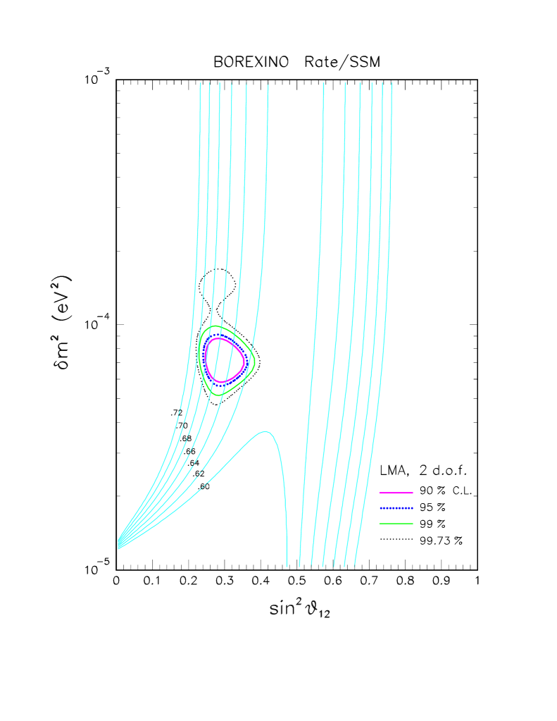
Figure 1: Suppression factor for the Borexino event rate, superposed to the current LMA allowed region.

The Borexino solar neutrino experiment (in construction) is expected to detect, in the absence of oscillations, about 55 events per day in the energy window $[0.25,0.80]$ MeV BORE . In the presence of oscillations, the rate suppression depends on the values of the dominant oscillation parameters $(\delta m^{2},\theta_{12})$. Figure 1 shows isolines of the the suppression factor in the mass-mixing plane, superposed to the current LMA solution to the solar neutrino problem (as taken from Ours ). From this figure we derive that the LMA-oscillated event rate in Borexino should be roughly equal to 13000 events per year, give or take one thousand events. After three years of data taking, the number of signal events should then be around

$$N_{S}\simeq 3.9\times 10^{4}\mathrm{\ (3\ years)}\ .$$ (19)

One of the goals of the Borexino experiment is to reach a background event rate comparable or smaller than the signal rate BORE ,

$$N_{B}/N_{S}\lesssim 1\ .$$ (20)

If such goal is achieved, from Eq. (12) we estimate that, after three years of data taking, the sensitivity to eccentricity effects should be definitely larger than $3\sigma$:

$$n_{\mathrm{sd}}\gtrsim 3.3\ .$$ (21)

Such “eccentricity test” will convincingly prove that the Borexino signal, despite the lack of directionality and the nonnegligible background-to-signal ratio, does come from solar neutrinos.

IV Testing day-night asymmetries

Within the current LMA solution to the solar neutrino problem (see Fig. 1), Earth matter effects Matt are expected to induce marginal day-night variations of the signal $S$ in the SK and SNO experiments (see, e.g., Pedr ; MSmy ; Petc ). Such effects, which decrease with increasing $\delta m^{2}/E_{\nu}$ (where $E_{\nu}$ is the neutrino energy), should be null in Borexino.

Earth matter effects are usually parametrized in terms of a day-night asymmetry $A$,

$$A=\frac{S_{n}-S_{d}}{\frac{1}{2}(S_{n}+S_{d})}$$ (22)

where $S_{n}$ and $S_{d}$ are the average signal event rates during night and day, respectively, with $S=(S_{d}+S_{n})/2$. Within the LMA solution it is $A>0$.

For our purposes, we can assume an approximate step-like variation of the signal as a function of the zenith angle $\theta_{z}$ (a variable more useful than the time $t$ in this context):

$$S(\cos\theta_{z})\simeq\left\{\begin{array}[]{lll}S(1-A/2)&\;,\;\cos\theta_{z}\in[-1,0]&\mathrm{(daytime)}\\ S(1+A/2)&\;,\;\cos\theta_{z}\in[0,+1]&\mathrm{(nighttime)}\\ \end{array}\right.$$ (23)

Within such approximation, the signal variance is simply given by

$$\frac{\sigma_{S}}{S}=\frac{A}{2}\ .$$ (24)

Using Eq. (10), the statistical significance of a day-night asymmetry $A$ is, in units of standard deviations,

$$n_{\mathrm{sd}}=\frac{A}{2}\sqrt{\frac{N_{S}}{1+N_{B}/N_{S}}}\ .$$ (25)

We shall use the above equation in a slightly different version, in order to estimate $\sigma_{A}$, namely, the $1\sigma$ statistical uncertainty of $A$. This uncertainty is obtained by setting $n_{\mathrm{sd}}=1$ and $A=\sigma_{A}$ in the above equation. The result,

$$\sigma_{A}=2\,\sqrt{\frac{1+N_{B}/N_{S}}{N_{S}}}$$ (26)

will be used for numerical estimates in SK, SNO, and Borexino.

IV.1 Application to SK

As in Sec. II A, we take for SK-I the values $N_{S}\simeq 22,400$ and $N_{B}/N_{S}\simeq 2.5$. Our estimate for the $1\sigma$ uncertainty of the day-night asymmetry $A$ is then

$$\sigma_{A}\simeq 2.5\times 10^{-2}\ ,$$ (27)

which is in reasonable agreement with the value $2.0\times 10^{-2}$ quoted by the SK Collaboration in Ref. MSmy for the “old” analysis method, based on the comparison of integrated daytime and nighttime samples.

In the same article MSmy , the SK collaboration also reported that, by using an extended maximum likelihood method, the statistical uncertainty of the day-night asymmetry can be reduced from $2.0\times 10^{-2}$ to $1.6\times 10^{-2}$, the latter being adopted as official SK value for $\sigma_{A}$. We interpret this reduction as an effective improvement in background rejection achieved through the SK maximum likelihood method (i.e., lower $N_{B}/N_{S}$ and thus lower $\sigma_{A}\propto\sqrt{1+N_{B}/N_{S}}$). We cannot further elaborate on this interpretation for lack of relevant information (the SK maximum likelihood analysis in MSmy is currently not reproducible outside the Collaboration); public release of such information would be beneficial to improve current global analyses of solar neutrino data, and to allow combined SK+SNO tests of day-night asymmetry effects (see also Sec. IV C).

IV.2 Application to SNO (phase I)

Table 1: SNO data from phase I (306.4 live days): Total number of events for each of the three classes CC, NC, ES and for the total solar neutrino signal $S$ (2nd column), together with their $\nu_{e}$ and $\nu_{\mu\tau}$ components for $\phi_{\mu\tau}/\phi_{e}=1.94$ (3rd and 4th column, respectively). See the text for details.

Class	Total events	$\nu_{e}$ component	$\nu_{\mu\tau}$ component
$X$	$N_{X}$	$N_{X}^{e}$	$N_{X}^{\mu\tau}$
CC	1967.7	1967.7	0
NC	576.5	196.3	380.2
ES	263.3	203.0	60.6
$S$	2807.8	2367.0	440.8

In its first phase of operation SNOD ; SNOA , the SNO detector has collected a total of $N_{S}=2807.8$ solar neutrino events with small background ($N_{B}/N_{S}=4.4\times 10^{-2}$, neglected in the following). The signal events are statistically separated into three classes (CC, NC, and ES), each class containing different contributions of events induced by $\nu_{e}$ and $\nu_{\mu,\tau}$. Table I shows the content of each class, as obtained by fixing the neutrino flux ratio $\phi_{\mu,\tau}/\phi_{e}=3.41/1.76=1.94$ and the cross-section ratio $\sigma_{\mu}/\sigma_{e}=1/6.48$ SNOD .

The SNO-I result for the day-night asymmetry of the $\nu_{e}$ component of the total signal ($A_{e}$) is SNOA

$$A_{e}=[7.0\pm 4.9\mathrm{(stat.)^{+1.3}_{-1.2}\mathrm{(syst.)}}]\times 10^{-2}\ ,$$ (28)

under the standard assumption of no asymmetry ($A=0$) for the total neutrino flux $\phi=\phi_{e}+\phi_{\mu\tau}$. In this section we reproduce with good accuracy the SNO-I statistical error estimate $\sigma_{A_{e}}=4.9\times 10^{-2}$. On the basis of this successful check, in the next Section we will try to estimate the value of $\sigma_{A_{e}}$ after the SNO I+II phases.

We remind that the $\nu_{e}$ and $\nu_{\mu\tau}$ components of the solar neutrino signal in SNO can be separated only on a statistical basis. Therefore, the $\nu_{e}$ asymmetry $A_{e}$ (which is not directly observable) must be linked to the day-night variation of the total signal $S$ (which is measurable), as described in the following.

The constraint of no day-night change for the total flux ($\phi_{e}+\phi_{\mu\tau}$) implies that the (approximately step-like) day-night variation of $\phi_{e}$,

$$\phi_{e}\to\phi_{e}\left(1\pm\frac{A_{e}}{2}\right)\ ,$$ (29)

is associated to the following day-night variation of $\phi_{\mu\tau}$,

$$\phi_{\mu\tau}\to\phi_{\mu\tau}\left(1\mp\frac{A_{e}}{2}\,\frac{\phi_{e}}{\phi_{\mu\tau}}\right)\ .$$ (30)

By applying the above variation factors to the $N_{S}^{e}$ and $N_{S}^{\mu\tau}$ components of the total number of solar neutrino events $N_{S}$, one gets the global day-night variation

$$N_{S}\to N_{S}\pm\frac{A_{e}}{2}\left(N_{e}-N_{\mu\tau}\frac{\phi_{e}}{\phi_{\mu\tau}}\right)\ ,$$ (31)

which, using the numbers in Table I (last row), provides the desired link between $A_{e}$ and the total signal variation,

$$N_{S}\to N_{S}\left(1\pm 0.76\,\frac{A_{e}}{2}\right)\ .$$ (32)

The analogous of Eq. (26) is then (for $N_{S}\simeq 2808$ and $N_{B}/N_{S}\ll 1$):

$$\sigma_{A_{e}}\simeq\frac{2}{0.76}\frac{1}{\sqrt{N_{S}}}=5.0\times 10^{-2}\ ,$$ (33)

in good agreement with the official SNO-I statistical error SNOA , also reported in Eq. (28). On the basis of this successful test, we “predict” in the next section the statistical error $\sigma_{A_{e}}$ expected from the day-night analysis of SNO I+II data.

IV.3 Application to SNO (phase I+II)

Table 2: SNO data from phases I+II ($306.4+254.2$ live days): Total number of events for each of the three classes CC, NC, ES and for the total solar neutrino signal $S$ (2nd column), together with their $\nu_{e}$ and $\nu_{\mu\tau}$ components (3rd and 4th column, respectively). See the text for details.

Class	Total events	$\nu_{e}$ component	$\nu_{\mu\tau}$ component
$X$	$N_{X}$	$N_{X}^{e}$	$N_{X}^{\mu\tau}$
CC	3307.3	3307.3	0
NC	1920.7	653.9	1266.8
ES	433.9	334.2	99.7
$S$	5661.9	4295.4	1366.5

In its second phase of operation SNON , the SNO detector has increased the solar neutrino statistics by $2854.1$ events, including 3307.3 CC, 1920.7 NC, and 433.9 ES events. Adding these events to those of phase I, one gets the total numbers reported in Table II (where, for the sake of simplicity, we have used the same $\phi_{\mu\tau}/\phi_{e}$ ratio as for the SNO phase I).

By inserting in Eq. (31) the values of $N^{e}_{S}$ and $N_{S}^{\mu\tau_{S}}$ from Table II, we get the following day-night variation for the total solar neutrino signal in SNO I+II ($N_{S}=5661.9$):

$$N_{S}\to N_{S}\left(1\pm 0.63\,\frac{A_{e}}{2}\right)\ ,$$ (34)

so that

$$\sigma_{A_{e}}\simeq\frac{2}{0.63}\frac{1}{\sqrt{N_{S}}}=4.3\times 10^{-2}\ .$$ (35)

Therefore, we estimate that the statistical error of the $\nu_{e}$ day-night asymmetry $A_{e}$ for SNO I+II should be about $4.3\times 10^{-2}$, i.e., not much smaller than for phase I only [see Eq. (28)]. Notice that, if the CC sample were hypothetically isolated on an event-by-event basis with no background (an irrealistic goal), the corresponding statistical uncertainty of the $\nu_{e}$ asymmetry would be $\sigma_{A_{\mathrm{CC}}}=2/\sqrt{N_{\mathrm{CC}}}=3.5\times 10^{-2}$ for SNO I+II. These considerations suggest that, in any case, the uncertainty of the $\nu_{e}$ day-night asymmetry in SNO I+II cannot be smaller than $\sim\!4\times 10^{-2}$. This statement will be checked soon, since the SNO I+II official day-night is currently being finalized Grah .

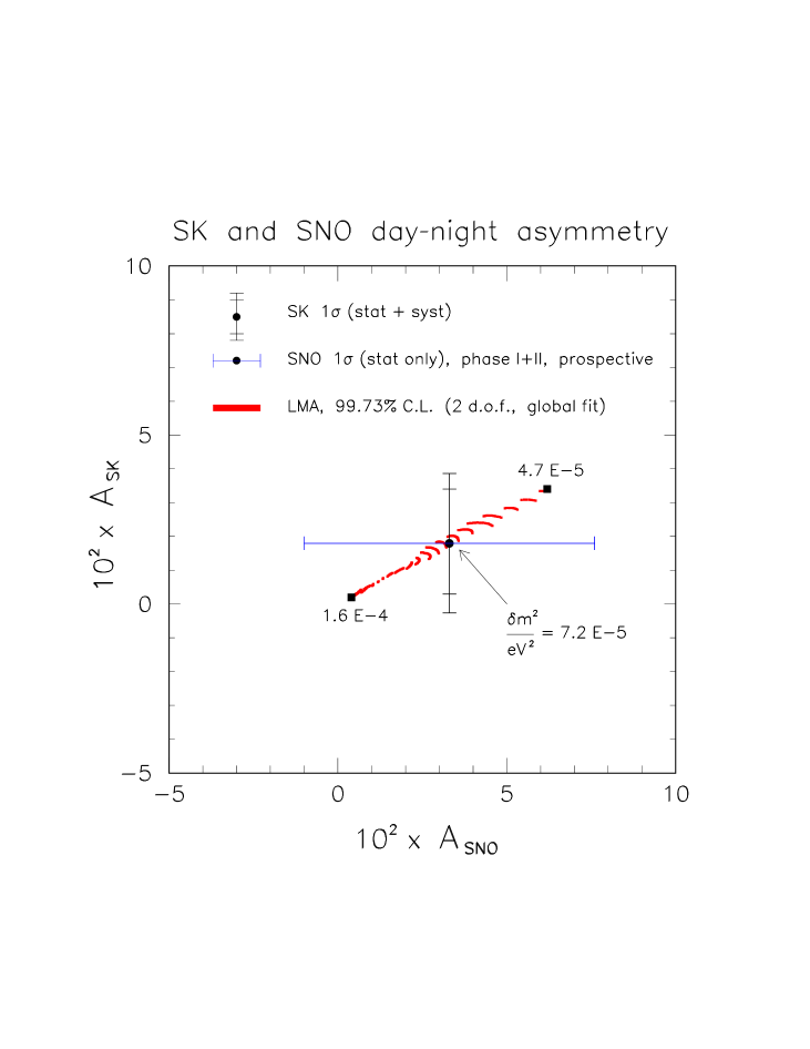
Figure 2: Correlation plot of the day-night asymmetry in SK and in SNO. The slanted region maps the LMA solution in Fig. 1 (at 99.73% C.L.), which strongly correlates the predictions for the day-night asymmetry in SK and SNO. Such predictions depend mainly on $\delta m^{2}$ (three representative values being shown in the figure). The datum with vertical errors bars ($\pm 1\sigma$ stat.+syst.) corresponds to the SK day-night measurement from MSmy . The “datum” with horizontal error bars implements our estimate for the day-night asymmetry uncertainty ($\pm 1\sigma$ stat. only) from prospective SNO I+II data ($306.4+254.2$ live days), with hypothetical best-fit central value.

Can the combination of the day-night asymmetries in SK (as reported in Ref. MSmy ) and in SNO I+II [our estimated error in Eq. (35)] improve the current determination of the LMA oscillation parameters? The answer can be derived from Fig. 2, where we map the current LMA region at 99.73% C.L. (as taken from Ours ) onto the plane charted by the SK and SNO day-night asymmetries. There is a strong positive correlations between the SK and SNO asymmetries, as it was emphasized in Ref. Corr and subsequently in Ref. Kras . The asymmetry rapidly decreases for increasing values of the neutrino squared mass difference $\delta m^{2}$, for which three representative values are shown in Fig. 2 (including the LMA best fit, $\delta m^{2}=7.2\times 10^{-5}$ eV² Ours ). On top of the LMA region, we superpose the SK day-night measurement at $\pm 1\sigma$ from MSmy , plus a prospective SNO I+II measurement characterized by our estimate for the statistical error [Eq. (35) and no systematic error], and by the “luckiest” central value (on top of the LMA best fit point). It can be seen that the SK+SNO “error box” at $\pm 1\sigma$ is larger than the current LMA region at 99.73% C.L. Therefore, although the combination of latest day-night asymmetry datum from SK MSmy and of the prospective one from SNO I+II (our estimate) can provide a useful consistency check of the LMA predictions, we do not expect that such data can significantly reduce the current LMA parameter region.

IV.4 Application to Borexino

In Borexino, one expects no day-night asymmetry ($A=0$) within the LMA solution to the solar neutrino problem. Using Eq. (26) and the same input values as in Sec. II C ($N_{S}=3.9\times 10^{4}$ and $N_{S}/N_{B}\lesssim 1$), we estimate the accuracy of this null result to be at least

$$A\pm\sigma_{A}=(0.0\pm 1.4)\times 10^{-2}\ ,$$ (36)

after three years of data taking. A check of the null result ($A=0$) with percent accuracy will provide a useful test that the Borexino detector works as expected, although it will not improve the determination of the neutrino oscillation parameters in the LMA region.

V Testing reactor power variations in KamLAND

The KamLAND experiment KLde ; Land is collecting events induced by $\bar{\nu}_{e}$ produced in (mainly) Japanese reactors. The reactor power demand (and thus the neutrino flux) in a given country generally follows a seasonal trend Grat . On top of this trend, a strong temporary reduction of Japanese reactors’ power has occurred at the end of 2002 and in 2003 Hort . Figure 3 (graphically reduced from Hort ) shows the total reactor fission flux during 540 days of KamLAND operation (starting on March 4, 2002), where the first 216 days correspond to the first phase with published results Land . In the following, we investigate whether such flux variations are detectable with 540-day statistics, with or without background, by using Eq. (10).

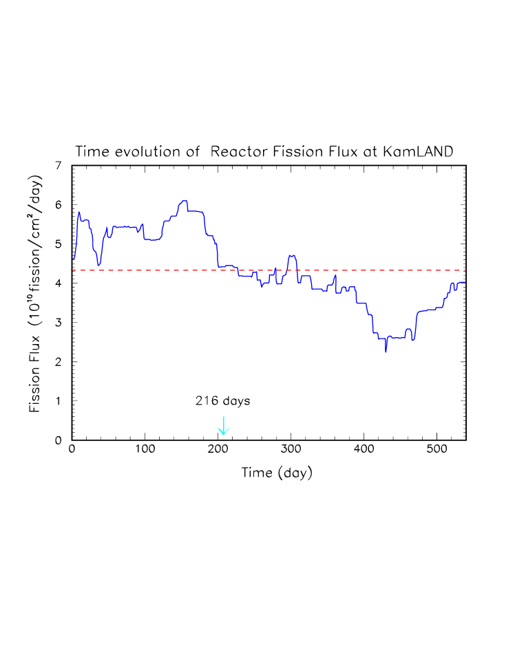
Figure 3: Variations of the total reactor fission flux power in KamLAND during 540 days of operation (as taken from Hort . The horizontal dashed line represents the average flux in the whole period. Published KamLAND data Land refer to the first 216 days.

V.1 Case without background

In the first 216 days, the KamLAND experiment has collected 54 events above the 2.6 MeV analysis threshold, which cuts away basically all backgrounds Land . If we naively rescale these events using the time variation curve in Fig. 3, we estimate that the statistics should be approximately doubled after 540 days,

$$N_{S}\simeq 2\times 54=108\ .$$ (37)

From the same curve in Fig. 3, we obtain that

$$\frac{\sigma_{S}}{S}\simeq 0.22$$ (38)

over the whole period. Therefore, we estimate that the KamLAND experiment should see an indication for reactor flux variations with a statistical significance equal to

$$n_{\mathrm{sd}}=\frac{\sigma_{S}}{S}\sqrt{N_{S}}\simeq 2.3$$ (39)

standard deviations, after 540 days of operation.

V.2 Case with background from geoneutrinos or from a georeactor

Below the 2.6 analysis threshold, the main irreducible known background in KamLAND is due to geoneutrinos Land . Since geo-$\bar{\nu}_{e}$ background predictions are uncertain Fior , we adopt for reference the KamLAND best-fit estimate of $N_{B}\simeq 9$ geoneutrino events, to be compared with the total reactor signal with no threshold, $N_{S}\simeq 71$ events Land .

The previous numbers refer to the first 216 days. At the end of 540 days of operation, the total reactor signal should be about doubled (as noted previously),

$$N_{S}\simeq 142\ ,$$ (40)

while the constant geoneutrino background should be rescaled by a factor $540/216=2.5$,

$$N_{B}\simeq 22.5\ .$$ (41)

Inserting these numbers [and Eq. (38)] in Eq. (10), one gets

$$n_{\mathrm{sd}}\simeq 2.4\ ,$$ (42)

which is comparable to the no-background estimate in Eq. (39). Reactor flux variations can thus be tested at $>2\sigma$ (after 540 days) also in the presence of geo-$\bar{\nu}_{e}$ background.

While geoneutrinos represent a “guaranteed” $\bar{\nu}_{e}$ background, a natural reactor $\bar{\nu}_{e}$ source in the Earth’s core (“georeactor”) Hern represents a more speculative hypothesis, which is not endorsed by standard geochemical Earth models (see, e.g., Dono ). For the sake of curiosity, we estimate that — as a rule of thumb — a georeactor of power $p$ (in units of TW) should add a fraction of about $p\%$ to the average KamLAND signal from man-made reactors. Assuming then a maximum power $p\simeq 10$ TW Hern , the additional georeactor background ($N_{B}/N_{S}\simeq 0.1$) should degrade the statistical significance estimated in Eqs. (39) and (42) by $\sim\!0.1\sigma$ or less. We conclude that, with or without geoneutrino or georeactor backgrounds, the KamLAND experiment should definitely be able to see time variations of the reactor signal at a level $\gtrsim 2\sigma$ (after 540 days of operation). This check will provide further confidence on the origin of the signal from reactor power plants.

If time variations of the reactor neutrino signal are successfully tested in KamLAND, one could, in principle, turn the test around, and try to constrain the amplitude of constant backgrounds such as geoneutrino or georeactor events. This kind of tests, together with detailed analyses of energy spectra, might improve the discrimination of man-made reactor signals from geo-signals. Such analyses could be performed also outside the Collaboration, provided that: (1) the neutrino flux “history” of each single reactor is publicly released, as it was emphasized in Lisi ; (2) the energy and time tag of each event (background and signal) is also released. The second condition is particularly important to perform unbinned data analyses in the geoneutrino energy window, where the few events being collected contain very precious information for Earth sciences. We hope that the KamLAND Collaboration will take these two desiderata into account.

VI Summary and Conclusions

Real-time neutrino oscillation experiments such as SK, SNO, Borexino, and KamLAND, can detect time variations of the incoming neutrino flux. We have introduced and discussed a possible test for time variations, which does not require time-binning of the events. The test provides a simple estimate for the statistical sensitivity to time variations, in terms of the signal variance and of total number of signal and background events [Eq. (10)]. This result has been used to discuss the significance of eccentricity effects and day-night variations in the SK, SNO, and Borexino solar neutrino experiments, as well as the sensitivity to reactor power variations in KamLAND. In particular, we estimate that: (1) the combination of SNO I+II data ($306.4+254.2$ live days) can provide indications for eccentricity effects at $>90\%$ C.L., but cannot provide a determination of the day-night asymmetry accurate enough to constrain significantly the current LMA allowed region of parameters, even in combination with current SK day-night data; (2) the Borexino experiment should test eccentricity effects at $>3\sigma$ in three years; and (3) the KamLAND experiment should already be able to test time variations of the reactor power at a level $>2\sigma$. Such estimates are statistical only, and should be somewhat degraded by systematic uncertainties, whose evaluation is beyond the scope of this work.

Appendix A Estimate of $\beta\pm\sigma_{\beta}$

In this Appendix we derive Eq. (9). We make use of the fact that, since

$$N=\int_{0}^{T}dt\,R(t)=N_{S}+N_{B}$$ (43)

and

$$N=\int_{0}^{T}dt\,\sum_{i=1}^{N_{S}+N_{B}}\delta(t-t_{i})$$ (44)

(where $\delta$ is a Dirac delta), we can formally write

$$dN=R(t)dt=\sum_{i=1}^{N_{S}+N_{B}}\delta(t-t_{i})\,dt\ .$$ (45)

This “trick” allows to express the continuous function $R(t)$ in terms of the discrete time series $\{t_{i}\}_{i=1,\dots,N_{S}+N_{B}}$, and to evaluate the variance of the small number $R(t)dt$ through Poisson’s statistics (see also Faid ):

$$\mathrm{var}(R(t)dt)=\mathrm{var}(dN)=dN=R(t)dt\ .$$ (46)

Let us prove that $\beta=N_{S}\sigma_{S}/S$:

$$\beta = \sum_{i=1}^{N_{S}+N_{B}}f(t_{i})$$ (47)

$$= \int_{0}^{T}dt\sum_{i=1}^{N_{S}+N_{B}}f(t)\,\delta(t-t_{i})$$ (48)

$$= \int_{0}^{T}dt\,R(t)\,f(t)$$ (49)

$$= \int_{0}^{T}dt\,\left[S\left(1+\frac{\sigma_{S}}{S}f(t)\right)+B\right]f(t)$$ (50)

$$= \int_{0}^{T}dt\,\sigma_{S}\,f^{2}(t)$$ (51)

$$= \sigma_{S}\,T$$ (52)

$$= \sigma_{S}\frac{N_{S}}{S}\ .$$ (53)

Finally, let us prove that, for $\sigma_{S}/S\ll 1$, it is $\sigma_{\beta}\simeq\sqrt{N_{S}+N_{B}}$:

$$\sigma^{2}_{\beta} = \mathrm{var}(\beta)$$ (54)

$$= \mathrm{var}\left(\int_{0}^{T}dt\,R(t)\,f(t)\right)$$ (55)

$$= \int_{0}^{T}dt\,f^{2}(t)\,R(t)$$ (56)

$$= (S+B)T+ST\frac{\sigma_{S}}{S}\left[\frac{1}{T}\int dt\,f^{3}(t)\right]$$ (57)

$$\simeq (S+B)T$$ (58)

$$= N_{S}+N_{B}$$ (59)

In deriving Eq. (56), we have used both the distributive property $\mathrm{var}(\sum_{i}a_{i}x_{i})=\sum_{i}a^{2}_{i}\mathrm{var}(x_{i})$ and Eq. (46). In deriving Eq. (58), we have dropped the second term on the right-hand-side of Eq. (57), which is not only of $O(\sigma_{S}/S)<1$ but, in typical applications (including all those considered in this work), is further suppressed by the small value of the third moment of $f(t)$.

Appendix B Relation with the Kolmogorov-Smirnov unbinned test

The Kolmogorov-Smirnov (KS) unbinned test can be used to compare two distributions through the maximal difference between their cumulative distributions Stat . In our case, the two distributions would be the total event rate $R(t)$ including time variations [Eqs. (3) and (4)] and the total event rate excluding time variations, $R_{0}=S+B$. It is easy to convince oneself that, in general, the maximal difference $d$ between the corresponding cumulative distributions is of the kind:

$$d=\eta\frac{\sigma_{S}}{S}\frac{N_{S}}{N_{S}+N_{B}}\ ,$$ (60)

where $\eta$ is a dimensionless factor of $O(1)$, which depends on the functional form of $f(t)$. The KS test then “measures” the difference $d$ in units of $\kappa/\sqrt{N}$ (for large $N=N_{S}+N_{B}$), where the number $\kappa$ depends on the confidence level chosen Stat . Therefore, the statistical significance of the KS test is proportional to

$$\frac{d\sqrt{N}}{\kappa}\propto\frac{\sigma_{S}}{S}\frac{N_{S}}{\sqrt{N_{S}+N_{B}}}\ .$$ (61)

The comparison of the above result with Eq. (10) suggests that the statistical significance of time variations should scale with $(\sigma_{S}/S)/(N_{S}/\sqrt{N_{S}+N_{B}})$, independently of the specific (unbinned) statistical test chosen—a fact than can be useful in prospective studies of experimental sensitivities. Different tests may differ, however, in statistical power. In all the examples discussed in this work, the KS test happens to be less powerful than the one proposed through Eq. (10), although we cannot exclude that it might be more powerful in other cases.

References

- (1) A.B. McDonald, C. Spiering, S. Schonert, E.T. Kearns, and T. Kajita, Rev. Sci. Instrum. 75, 293 (2004).
- (2) SK Collaboration, Y. Fukuda et al., Nucl. Instrum. Meth. A 501, 418 (2003).
- (3) SNO Collaboration, J. Boger et al., Nucl. Instrum. Meth. A 449, 172 (2000).
- (4) KamLAND Collaboration, D.M. Markoff et al., J. Phys. G 29, 1481 (2003).
- (5) Borexino Collaboration, G. Alimonti et al., Astropart. Phys. 16, 205 (2002).
- (6) G.L. Fogli, E. Lisi and D. Montanino, Phys. Rev. D 56, 4374 (1997).
- (7) B. Faïd, G.L. Fogli, E. Lisi and D. Montanino, Astropart. Phys. 10, 93 (1999).
- (8) SK Collaboration, J. Yoo et al., Phys. Rev. D 68, 092002 (2003).
- (9) P.C. de Holanda and A.Yu. Smirnov, hep-ph/0309299.
- (10) SK Collaboration, M.B. Smy et al., Phys. Rev. D 69, 011104 (2004).
- (11) SK Collaboration, S. Fukuda et al., Phys. Rev. Lett. 86, 5651 (2001).
- (12) SNO Collaboration, Q.R. Ahmad et al., Phys. Rev. Lett. 87, 071301 (2001).
- (13) SNO Collaboration, Q.R. Ahmad et al., Phys. Rev. Lett. 89, 011301 (2002).
- (14) SNO Collaboration, Q.R. Ahmad et al., Phys. Rev. Lett. 89, 011302 (2002).
- (15) SNO Collaboration, S.N. Ahmed et al., nucl-ex/0309004.
- (16) G.L. Fogli, E. Lisi, A. Marrone, and A. Palazzo, Phys. Lett. B 583, 149 (2004).
- (17) L. Wolfenstein, Phys. Rev. D 17, 2369 (1978); S.P. Mikheev and A.Yu. Smirnov, Yad. Fiz. 42, 1441 (1985) [Sov. J. Nucl. Phys. 42, 913 (1985)].
- (18) A. Bandyopadhyay, S. Choubey, S. Goswami, S.T. Petcov, and D.P. Roy, Phys. Lett. B 583, 134 (2004).
- (19) K. Graham for the SNO Collaboration, talk given at NOON 2004, 5th International Workshop on Neutrino Oscillations and their OrigiN (Tokyo, Japan, 2004); website: www-sk.icrr.u-tokyo.ac.jp/noon2004 .
- (20) G.L. Fogli, E. Lisi, and D. Montanino, Phys. Lett. B 434, 333 (1998).
- (21) J.N. Bahcall, P.I. Krastev, and A.Yu. Smirnov, Phys. Rev. D 62, 093004 (2000); ibidem 63, 053012 (2001).
- (22) KamLAND Collaboration, K. Eguchi et al., Phys. Rev. Lett. 90, 021802 (2003).
- (23) C. Bemporad, G. Gratta, and P. Vogel, Rev. Mod. Phys. 74, 297 (2002).
- (24) G.A. Horton-Smith for the KamLAND Collaboration, talk given at NO-VE 2003, 2nd International Workshop on Neutrino Oscillations in Venice (Venice, Italy, 2003); website: axpd24.pd.infn.it/NO-VE/NO-VE.html
- (25) F. Mantovani, L. Carmignani, G. Fiorentini, and M. Lissia, Phys. Rev. D 69, 013001 (2004).
- (26) J.M. Herndon, Proc. Natl. Acad. Sci. U.S.A. 93(2), 646 (1996); ibidem 100(6), 3047 (2003); see also the website www.nuclearplanet.com .
- (27) W.F. McDonough, Compositional Models for the Earth’s Core, in “Treatise on Geochemistry,” Vol. II, edited by R.W. Carlson (Elsevier Science, Amsterdam, 2003); website www.treatiseongeochemistry.com .
- (28) E. Lisi, talk at NOON 2003, 4th International Workshop on Neutrino Oscillations and their OrigiN (Kanazawa, Japan, 2003); website: www-sk.icrr.u-tokyo.ac.jp/noon2003 .
- (29) W.T. Eadie, D. Drijard, F.E. James, M. Roos, and B. Sadoulet, Statistical Methods in Experimental Physics (North-Holland, Amsterdam, 1971).