Radiative $B$ decays to the axial $K$ mesons at next-to-leading order

Abstract

We calculate the branching ratios of $B\to K_{1}\gamma$ at next-to-leading order (NLO) of $\alpha_{s}$ where $K_{1}$ is the orbitally excited axial vector meson. The NLO decay amplitude is divided into the vertex correction and the hard spectator interaction part. The one is proportional to the weak form factor of $B\to K_{1}$ transition while the other is a convolution between light-cone distribution amplitudes and hard scattering kernel. Using the light-cone sum rule results for the form factor, we have ${\cal B}(B^{0}\to K_{1}^{0}(1270)\gamma)=(0.828\pm 0.335)\times 10^{-5}$ and ${\cal B}(B^{0}\to K_{1}^{0}(1400)\gamma)=(0.393\pm 0.151)\times 10^{-5}$.
PACS: 13.20.He, 12.38.Bx

I Introduction

Radiative $B$ decays into Kaons provide abundant issues for both theorists and experimentalists. After the first measurement at CLEO, $B\to K^{*}\gamma$ is now also measured in Belle and BaBar:

$${\cal B}(B^{0}\to K^{*0}\gamma) = \left\{\begin{array}[]{cc}(4.09\pm 0.21\pm 0.19)\times 10^{-5}&{\rm Belle}~{}\cite[cite]{[\@@bibref{Number}{Belle}{}{}]}\\ (4.23\pm 0.40\pm 0.22)\times 10^{-5}&{\rm BaBar}~{}\cite[cite]{[\@@bibref{Number}{BaBar}{}{}]}\\ (4.55\pm 0.70\pm 0.34)\times 10^{-5}&{\rm CLEO}~{}\cite[cite]{[\@@bibref{Number}{CLEO}{}{}]}\end{array}\right.~{},$$ (4)

$${\cal B}(B^{+}\to K^{*+}\gamma) = \left\{\begin{array}[]{cc}(4.40\pm 0.33\pm 0.24)\times 10^{-5}&{\rm Belle}~{}\cite[cite]{[\@@bibref{Number}{Belle}{}{}]}\\ (3.83\pm 0.62\pm 0.22)\times 10^{-5}&{\rm BaBar}~{}\cite[cite]{[\@@bibref{Number}{BaBar}{}{}]}\\ (3.76\pm 0.86\pm 0.28)\times 10^{-5}&{\rm CLEO}~{}\cite[cite]{[\@@bibref{Number}{CLEO}{}{}]}\end{array}\right.~{}.$$ (8)

Theoretical advances in $B\to K^{*}\gamma$ have been noticeable for a decade. QCD corrections at next-to-leading order (NLO) of ${\cal O}(\alpha_{s})$ was already considered in [4, 5, 6]. Furthermore, relevant Wilson coefficients have been improved [7, 8] up to three-loop calculations. Recent developments of the QCD factorization [9] helped one calculate the hard spectator contributions systematically in a factorized form through the convolution at the heavy quark limit [10, 11, 12]. $B\to K^{*}\gamma$ is also analyzed in the effective theories at NLO, such as large energy effective theory [13] and the soft-collinear effective theory (SCET) [14].

In addition to $K^{*}$, higher resonances of Kaon also deserve much attention. Especially, it was suggested that $B\to K_{\rm res}(\to K\pi\pi)\gamma$ can provide a direct measurement of the photon polarization [15]. In particular, it was shown that $B\to K_{1}(1400)\gamma$ can produce large polarization asymmetry of $\approx 33\%$ in the standard model. In the presence of anomalous right-handed couplings, the polarization can be severely reduced in the parameter space allowed by current experimental bounds of $B\to X_{s}\gamma$ [16]. It was also argued that the $B$ factories can now make a lot of $B{\bar{B}}$ pairs enough to check the anomalous couplings through the measurement of the photon polarization.

As for the axial $K_{1}$, unfortunately, current measurements give only upper bounds for $B\to K_{1}\gamma$ [17]:

$${\cal B}(B^{+}\to K_{1}^{+}(1270)\gamma) < 9.9\times 10^{-5}~{},$$ (9)

$${\cal B}(B^{+}\to K_{1}^{+}(1400)\gamma) < 5.0\times 10^{-5}~{}.$$ (10)

For the decays of $B\to K_{2}(1430)\gamma$, CLEO and the $B$ factories have reported the branching ratios

$${\cal B}(B\to K_{2}^{*}\gamma) = (1.66^{+0.59}_{-0.53}\pm 0.13)\times 10^{-5}~{}{\rm CLEO}~{}\cite[cite]{[\@@bibref{Number}{CLEO}{}{}]}~{},$$ (11)

$${\cal B}(B^{0}\to K_{2}^{*0}\gamma) = \left\{\begin{array}[]{cc}(1.3\pm 0.5\pm 0.1)\times 10^{-5}&{\rm Belle}~{}\cite[cite]{[\@@bibref{Number}{Belle2}{}{}]}\\ (1.22\pm 0.25\pm 0.11)\times 10^{-5}&{\rm BaBar}~{}\cite[cite]{[\@@bibref{Number}{BaBar2}{}{}]}\end{array}\right.~{},$$ (14)

$${\cal B}(B^{+}\to K_{2}^{*+}\gamma) = (1.44\pm 0.40\pm 0.13)\times 10^{-5}~{}{\rm BaBar}~{}\cite[cite]{[\@@bibref{Number}{BaBar2}{}{}]}~{}.$$ (15)

Since the higher resonant Kaons are rather heavy $\gtrsim 1~{}{\rm GeV}$, it is quite natural and attractive to consider them as heavy mesons. The advent of heavy quark effective theory (HQET) provoked many studies. Although the HQET simplifies the analysis by reducing number of the independent form factors involved, other non-perturbative methods are needed to complete the phenomenological explanation. These HQET-based analyses include HQET-ISGW (Isgur-Scora-Grinstein-Wise) [19] and HQET-NRQM (Non-Relativistic Quark Model) [20]. Other model calculations have been done in [21, 22, 23, 24].

In this paper, the branching ratios of $B\to K_{1}\gamma$ at NLO of $\alpha_{s}$ are calculated. We adopt the QCD factorization framework where the hard spectator interactions are described by the convolution between the hard-scattering kernel and the lint-cone distribution amplitudes (DA) at the heavy quark limit. All the non-perturbative nature are encapsulated in the DA while the hard kernel is perturbatively calculable. Basically, $B\to K_{1}\gamma$ shares many things with $B\to K^{*}\gamma$. Only the difference is the DA for the daughter mesons. Vector and axial vector mesons are distinguished by the $\gamma_{5}$ in the gamma structure of DA and some non-perturbative parameters. But the presence of $\gamma_{5}$ does not alter the calculation, giving the same result for the perturbative part. As for the non-perturbative parameters, the decay constant is most important. If higher twist terms are included, the Gegenbauer moments in the Gegenbauer expansion are also process dependent. We will not consider higher twists for simplicity.

Another NLO contributions are the vertex corrections to the relevant operators. They are all proportional to the leading operator $O_{7}$. The matrix elements of $O_{7}$ are parameterized by several form factors. For the radiative decays where the emitted photons are real, only one form factor enters the decay amplitude. However, other non-perturbative calculation is needed for the value of the form factor. We use the light-cone sum rule (LCSR) results for it [25].

Thus at NLO, $B\to K^{*}\gamma$ and $B\to K_{1}\gamma$ are characterized by the weak form factor $F^{V(A)}_{+}$ and decay constant, plugged by the common perturbative and kinematical factors. With ${\cal B}(B\to K^{*}\gamma)$ at hand, near future measurements of $B\to K_{1}\gamma$ will check this structure.

The paper is organized as follows. General setup and leading contribution to $B\to K_{1}\gamma$ are given in the next Section. Section III is devoted to the NLO corrections. The resulting branching ratios and related discussions appear in Sec. IV. We conclude in Sec. V.

II Leading order contribution

Let us start with the effective Hamiltonian for $b\to s\gamma$,

$${\cal H}_{\rm eff}(b\to s\gamma)=-\frac{G_{F}}{\sqrt{2}}V_{tb}V_{ts}^{*}\sum_{i=1}^{8}C_{i}(\mu)O_{i}(\mu)~{},$$ (16)

where

$$O_{1} = ({\bar{s}}_{i}c_{j})_{V-A}({\bar{c}}_{j}b_{i})_{V-A}~{},$$ (17)

$$O_{2} = ({\bar{s}}_{i}c_{i})_{V-A}({\bar{c}}_{j}b_{j})_{V-A}~{},$$ (18)

$$O_{3} = ({\bar{s}}_{i}b_{i})_{V-A}\sum_{q}({\bar{q}}_{j}q_{j})_{V-A}~{},$$ (19)

$$O_{4} = ({\bar{s}}_{i}b_{j})_{V-A}\sum_{q}({\bar{q}}_{j}q_{i})_{V-A}~{},$$ (20)

$$O_{5} = ({\bar{s}}_{i}b_{i})_{V-A}\sum_{q}({\bar{q}}_{j}q_{j})_{V+A}~{},$$ (21)

$$O_{6} = ({\bar{s}}_{i}b_{j})_{V-A}\sum_{q}({\bar{q}}_{j}q_{i})_{V+A}~{},$$ (22)

$$O_{7} = \frac{em_{b}}{8\pi^{2}}{\bar{s}}_{i}\sigma^{\mu\nu}(1+\gamma_{5})b_{i}F_{\mu\nu}~{},$$ (23)

$$O_{8} = \frac{g_{s}m_{b}}{8\pi^{2}}{\bar{s}}_{i}\sigma^{\mu\nu}(1+\gamma_{5})T^{a}_{ij}b_{j}G^{a}_{\mu\nu}~{}.$$ (24)

Here $i,j$ are color indices, and we neglect the CKM element $V_{ub}V_{us}^{*}$ as well as the $s$-quark mass. The leading contribution to $B\to K_{1}\gamma$ comes from the electromagnetic operator $O_{7}$ as shown in Fig. 1. The matrix element of $O_{7}$ is described by the transition form factors $F^{A}_{\pm,0}$ which are defined by

$$\langle K_{1}(p^{\prime},\epsilon)|{\bar{s}}i\sigma_{\mu\nu}q^{\nu}b|B(p)\rangle$$ (26)

$$= F^{A}_{+}(q^{2})\Big{[}(\epsilon^{*}\cdot q)(p+p^{\prime})_{\mu}-\epsilon^{*}_{\mu}(p^{2}-p^{\prime 2})\Big{]}+F^{A}_{-}(q^{2})\Big{[}(\epsilon^{*}\cdot q)q_{\mu}-\epsilon^{*}_{\mu}q^{2}\Big{]}$$ (28)

$$+\frac{F^{A}_{0}(q^{2})\epsilon^{*}\cdot q}{m_{B}m}\Big{[}(p^{2}-p^{\prime 2})q_{\mu}-(p+p^{\prime})_{\mu}q^{2}\Big{]}~{},$$

$$\langle K_{1}(p^{\prime},\epsilon)|{\bar{s}}i\sigma_{\mu\nu}\gamma_{5}q^{\nu}b|B(p)\rangle=iF^{A}_{+}(q^{2})\epsilon_{\mu\nu\alpha\beta}\epsilon^{*\nu}q^{\alpha}(p+p^{\prime})^{\beta}~{},$$ (29)

where $m$ and $\epsilon^{\mu}$ are the mass and polarization vector of $K_{1}$, respectively, and $q=p-p^{\prime}$ is the photon momentum. In case of real photon emission ($q^{2}=0$), only $F^{A}_{+}$ is involved as

$$\langle O_{7}\rangle_{A} \equiv \langle K_{1}(p^{\prime},\epsilon)\gamma(q,e)|O_{7}|B(p)\rangle$$ (30)

$$= \frac{em_{b}}{4\pi^{2}}F^{A}_{+}(0)\Big{[}\epsilon^{*}\cdot q(p+p^{\prime})\cdot e^{*}-\epsilon^{*}\cdot e^{*}(p^{2}-p^{\prime 2})+i\epsilon_{\mu\nu\alpha\beta}e^{*\mu}\epsilon^{*\nu}q^{\alpha}(p+p^{\prime})^{\beta}\Big{]}~{},$$ (31)

with $e^{\mu}$ being the photon polarization vector. The decay rate is straightforwardly obtained to be

$$\Gamma(B\to K_{1}\gamma)=\frac{G_{F}^{2}\alpha m_{b}^{2}m_{B}^{3}}{32\pi^{4}}|V_{tb}V_{ts}^{*}|^{2}\Bigg{(}1-\frac{m^{2}}{m_{B}^{2}}\Bigg{)}^{3}|F^{A}_{+}|^{2}|C_{7}^{\rm eff(0)}|^{2}~{},$$ (32)

where $\alpha$ is the fine-structure constant and $C_{7}^{\rm eff(0)}$ is the effective Wilson coefficient at leading order.

III Matrix elements at next-to-leading order of ${\cal O}(\alpha_{s})$

At next-to-leading order of $\alpha_{s}$, there are other contributions from the operators $O_{2}$ and $O_{8}$. We simply neglect the annihilation topologies. Explicitly, the decay amplitude ${\cal A}$ is given by

$${\cal A}(B\to K_{1}\gamma)=-\frac{G_{F}}{\sqrt{2}}V_{tb}V_{ts}^{*}(C_{7}^{\rm eff}\langle O_{7}\rangle+C_{2}\langle O_{2}\rangle+C_{8}^{\rm eff}\langle O_{8}\rangle)~{},$$ (33)

where $\langle O_{i}\rangle\equiv\langle K_{1}\gamma|O_{i}|B\rangle$. Every $\langle O_{i}\rangle$ has its vertex correction $\langle O_{i}\rangle_{VC}$ and hard spectator interaction term $\langle O_{i}\rangle_{HS}$ as shown in Figs. 2 and 3;

$$\langle O_{i}\rangle=\langle O_{i}\rangle_{VC}+\langle O_{i}\rangle_{HS}~{}.$$ (34)

As for $\langle O_{7}\rangle$, all the subleading contributions shown in Fig. 2 are absorbed into the form factor $F^{A}_{+}$ while the corresponding Wilson coefficient $C_{7}^{\rm eff}$ contains its NLO part,

$$C_{7}^{\rm eff}(\mu)=C_{7}^{\rm eff(0)}(\mu)+\frac{\alpha_{s}(\mu)}{4\pi}C_{7}^{\rm eff(1)}(\mu)~{}.$$ (35)

On the other hand, the leading order $C_{2}^{(0)}$ and $C_{8}^{\rm eff(0)}$ are sufficient for $C_{2}$ and $C_{8}$ since $O_{2}$ and $O_{8}$ contributions begin at NLO.

The vertex corrections are directly proportional to the form factor $F^{A}_{+}$. They are given by (Fig. 3) [6, 8]

$$\langle O_{2}\rangle_{VC} = \frac{\alpha_{s}}{4\pi}\langle O_{7}\rangle\Bigg{(}\frac{416}{81}\ln\frac{m_{b}}{\mu}+r_{2}\Bigg{)}~{},$$ (36)

$$\langle O_{8}\rangle_{VC} = \frac{\alpha_{s}}{4\pi}\langle O_{7}\rangle\Bigg{[}-\frac{32}{9}\ln\frac{m_{b}}{\mu}+\frac{4}{27}(33-2\pi^{2}+6i\pi)\Bigg{]}~{},$$ (37)

where

$$r_{2} = \frac{2}{243}\Big{\{}-833+144\pi^{2}z^{3/2}$$ (41)

$$+\Big{[}1728-180\pi^{2}-1296\zeta(3)+(1296-324\pi^{2})L+108L^{2}+36L^{3}\Big{]}z$$

$$+\Big{[}648+72\pi^{2}+(432-216\pi^{2})L+36L^{3}\Big{]}z^{2}+\Big{[}-54-84\pi^{2}+1092L-756L^{2}\Big{]}z^{3}\Bigg{\}}$$

$$+i\frac{16\pi}{81}\Bigg{\{}-5+\Big{[}45-3\pi^{2}+9L+9L^{2}\Big{]}z+\Big{[}-3\pi^{2}+9L^{2}\Big{]}z^{2}+\Big{[}28-12L\Big{]}z^{3}\Bigg{\}}~{},$$

with $z\equiv m_{c}^{2}/m_{b}^{2}$, $L\equiv\ln z$, and $\zeta(x)$ being the Liemann $\zeta$-function.

Hard spectator corrections are well described by the convolution between the hard kernel $T_{i}(\xi,u)$ and the light-cone distribution amplitudes of the involved mesons, $\Phi_{B}(\xi)$ and $\Phi_{A}(u)$, in the heavy quark limit;

$$\langle O_{i}\rangle_{HS}=\int_{0}^{1}d\xi du\Phi_{B}(\xi)T_{i}(\xi,u)\Phi_{A}(u)~{}.$$ (42)

The light-cone distribution amplitudes are defined by

$$\langle 0|b(0){\bar{q}}^{\prime}(z)|B(p)\rangle = \frac{if_{B}}{4}({p/}+m_{B})\gamma_{5}\int_{0}^{1}d\xi~{}e^{-i\xi p_{+}z_{-}}\Big{[}\Phi_{B1}(\xi)+{{\bar{n}}/}\Phi_{B2}(\xi)\Big{]}~{},$$ (44)

$$\langle A(p^{\prime},\epsilon)|q(z){\bar{q}}(0)|0\rangle = \frac{f_{A}^{\perp}}{4}\gamma_{5}\sigma^{\mu\nu}\epsilon_{\mu}p^{\prime}_{\nu}\int_{0}^{1}du~{}e^{i{\bar{u}}p^{\prime}\cdot z}\Phi_{A}^{\perp}(u)~{},~{}~{}~{}~{}~{}({\bar{u}}\equiv 1-u)$$ (45)

where ${\bar{n}}^{\mu}=(1,0,0,-1)$ is parallel to the outgoing meson. To calculate the hard spectator contributions, following kinematics for Fig. 2 is adopted:

$$p_{b}^{\mu} = m_{b}v^{\mu}~{},$$ (46)

$$l^{\mu} = \frac{l_{+}}{2}n^{\mu}+l^{\mu}_{\perp}+\frac{l_{-}}{2}{\bar{n}}^{\mu}~{},$$ (47)

$$q^{\mu} = \omega n^{\mu}~{}~{}~{}(\omega\simeq m_{B}/2)~{},$$ (48)

$$k_{1}^{\mu} \simeq uE{\bar{n}}^{\mu}+k_{\perp}^{\mu}+{\cal O}(k_{\perp}^{2})~{},$$ (49)

$$k_{2}^{\mu} \simeq {\bar{u}}E{\bar{n}}^{\mu}-k_{\perp}^{\mu}+{\cal O}(k_{\perp}^{2})~{}~{}~{}(E\simeq m_{B}/2)~{},$$ (50)

where $n^{\mu}=(1,0,0,1)$ and $u$ is the relative energy fraction.

Direct calculation of each diagram in Fig. 4 plugged with Eq. (III) yields

$$\langle O_{2}\rangle_{HS} = \frac{\langle O_{7}\rangle_{A}}{F^{A}_{+}(0)}\frac{4\pi\alpha_{s}C_{F}}{N_{c}}\frac{f_{B}f_{A}^{\perp}}{m_{b}m_{B}}\Bigg{[}\frac{1}{12}\langle u^{-1}\Delta F_{1}(z_{1}^{(c)})\rangle_{\perp}+\frac{3}{16}Q_{sp}\langle{\bar{u}}^{-1}\Delta F_{1}(z_{0}^{(c)})\rangle_{\perp}$$ (52)

$$-\frac{1}{12}\langle\xi^{-1}\rangle_{1}\langle{\bar{u}}^{-1}\Delta i_{5}(z_{0}^{(c)},z_{1}^{(c)},0)\rangle_{\perp}-\frac{1}{3}\langle{\bar{u}}^{-1}\Delta i_{25}(z_{0}^{(c)},z_{1}^{(c)},0)\rangle_{\perp}\Bigg{]}~{},$$

$$\langle O_{8}\rangle_{HS} = \frac{\langle O_{7}\rangle_{A}}{F^{A}_{+}(0)}\frac{4\pi\alpha_{s}C_{F}}{N_{c}}\frac{f_{B}f_{A}^{\perp}}{m_{B}^{2}}\Bigg{[}\frac{1}{12}\langle u^{-1}\rangle_{\perp}\langle\xi^{-1}\rangle_{1}+\frac{Q_{sp}}{8}(\langle{\bar{u}}^{-1}\rangle_{\perp}+2\langle{\bar{u}}^{-2}\rangle_{\perp})\Bigg{]}~{}.$$ (53)

Here $N_{c}$ is the number of color with $C_{F}=\frac{N_{c}^{2}-1}{2N_{c}}$, and $Q_{sp}$ is the electric charge of the spectator quark. The expectation values over the distribution amplitudes are defined by

$$\langle f(u)\rangle_{\perp} \equiv \int_{0}^{1}du~{}f(u)\Phi_{A}^{\perp}(u)~{},$$ (55)

$$\langle\xi^{N}\rangle_{1} \equiv \int_{0}^{1}d\xi~{}\xi^{N}\Phi_{B1}(\xi)~{}.$$ (56)

Relevant functions $\Delta F_{1}$, $\Delta i_{5}$, and $\Delta i_{25}$ as well as the arguments $z_{0,1}^{(f)}$ are given in [13, 26].

IV Branching ratios for $B\to K_{1}\gamma$

The branching ratio of $B\to K_{1}\gamma$ is simply given by

$${\cal B}(B\to K_{1}\gamma)=\tau_{B}\frac{G_{F}^{2}\alpha m_{b}^{2}m_{B}^{3}}{32\pi^{4}}\Bigg{(}1-\frac{m_{A}^{2}}{m_{B}^{2}}\Bigg{)}^{3}|F^{A}_{+}(0)|^{2}|V_{tb}V_{ts}^{*}|^{2}|C_{7}^{\rm eff}(\mu_{b})+A_{VC}+A_{HS}|^{2}~{}.$$ (57)

At the heavy quark limit,

$$A_{VC} = \frac{\alpha_{s}(\mu_{b})}{4\pi}\Bigg{\{}C_{8}^{\rm eff}(\mu_{b})\Bigg{[}-\frac{32}{9}\ln\frac{m_{b}}{\mu_{b}}+\frac{4}{27}(33-2\pi^{2}+6i\pi)\Bigg{]}+C_{2}(\mu_{b})\Bigg{[}\frac{416}{81}\ln\frac{m_{b}}{\mu_{b}}+r_{2}\Bigg{]}\Bigg{\}}~{},$$ (58)

$$A_{HS} = \frac{4\pi\alpha_{s}(\mu_{H})C_{F}}{N_{c}}\frac{f_{B}f_{A}^{\perp}}{\lambda_{B}m_{B}F^{A}_{+}(0)}\Bigg{\{}C_{8}^{\rm eff}(\mu_{H})\frac{1}{12}\langle u^{-1}\rangle_{\perp}-C_{2}(\mu_{H})\frac{1}{12}\left\langle\frac{\Delta i_{5}(z_{0}^{(c)},0,0)}{{\bar{u}}}\right\rangle_{\perp}\Bigg{\}}~{},$$ (59)

where the negative moment of $\Phi_{B1}$ is parameterized by $\lambda_{B}\sim{\cal O}(\Lambda_{\rm QCD})$ as

$$\int_{0}^{1}d\xi~{}\frac{\Phi_{B1}(\xi)}{\xi}\equiv\frac{m_{B}}{\lambda_{B}}~{}.$$ (60)

The renormalization scale is fixed at $\mu=\mu_{b}={\cal O}(m_{b})$ for the vertex corrections while for the hard spectator interactions, $\mu=\mu_{H}\sim\sqrt{\Lambda_{\rm QCD}m_{b}}$. In the following analysis, we set $\mu_{b}=m_{b}$ and $\mu_{H}=\sqrt{\Lambda_{H}m_{b}}$ where $\Lambda_{H}=0.5$ GeV.

The scale dependence of $\langle O_{7}\rangle$ is absorbed into the product of $b$-quark mass and the form factor; [12]

$$(m_{b}\cdot F^{A}_{+})[\mu]=(m_{b}\cdot F^{A}_{+})[m_{b}]\Bigg{(}1+\frac{\alpha_{s}(\mu)}{4\pi}\frac{32}{3}\ln\frac{m_{b}}{\mu}\Bigg{)}~{}.$$ (61)

Other input values are summarized in Table I. Contrary to the $B\to K^{*}\gamma$, there are few reliable values for $F^{A}_{+}(0)$ and $f_{A}^{\perp}$ both in theory and experiment in the literature. We adopt the results from the light-cone sum rules by Safir [25], whose values are listed in Table II. In Table III, each contributions to the decay amplitudes is listed from the central values of Tables I and II. Note that the NLO corrections contribute positively, except $C_{7}^{\rm eff(1)}$. Reference scale for the present analysis is

$$(\mu_{b},\mu_{H})=(m_{b}(m_{b}),\sqrt{\Lambda_{H}m_{b}(m_{b})})=(4.2~{}{\rm GeV},1.45~{}{\rm GeV})~{}.$$ (62)

As a comparison, results for another scale $(\mu_{b},\mu_{H})=(m_{b,PS},(m_{b}(m_{b}))$ are also given in Table III, where $m_{b,PS}=4.6$ GeV is the so-called potential-subtracted mass [27]. It should be emphasized that in Table III, $C_{7}^{\rm eff}$ and $A_{VC}$ are process independent, and encodes QCD effects only. On the other hand, $A_{HS}$ contains the key information of the outgoing meson. Although $F^{A}_{+}(0)$ in $A_{HS}$ is canceled, non-perturbative properties of daughter meson still remain in $f_{A}^{\perp}$ and $\langle\cdots\rangle_{\perp}$. When averaging over $\Phi_{A}^{\perp}(u)$, process dependence is encapsulated in the coefficients of the Gegenbauer expansion, which vanish at $\mu\to\infty$. We simply neglect the expansion here, retaining $\Phi_{A}^{\perp}$ as its asymptotic form

$$\Phi_{A}^{\perp}(u)\approx\Phi_{A}^{\perp(as)}(u)=6u{\bar{u}}~{}.$$ (63)

Keeping the hadronic parameters specifically, we have

$${\cal B}(B^{0}\to K_{1}^{0}\gamma) = 0.003\times\Bigg{(}1-\frac{m^{2}}{m_{B}^{2}}\Bigg{)}^{3}\times\left|F^{A}_{+}(0)(-0.385-i0.014)\right.$$ (65)

$$\left.+(f_{A}^{\perp}/{\rm GeV})(-0.024-i0.022)\right|^{2}~{}.$$

Final results for the decay amplitudes and the branching ratios are listed in Table IV. Uncertainties in the branching ratios are from those in the form factor. For the charged modes, one has only to multiply the life-time ratio $\tau_{B^{\pm}}/\tau_{B^{0}}$ to the above equation.

In Eq. (65), the coefficient of $F^{A}_{+}(0)$ is $C_{7}^{\rm eff}(\mu_{b})+A_{VC}(\mu_{b})$, while that of $f_{A}^{\perp}$ is $A_{HS}(\mu_{H})\times F^{A}_{+}(0)/f_{A}^{\perp}$. Since the presence of $\gamma_{5}$ in Eq. (45) does not change the trace calculation for getting Eq. (52) and the form of $\Phi_{A}^{\perp(as)}$ is universal, the numerics in Eq. (65) are common to both $B\to K_{V}\gamma$ and $B\to K_{A}\gamma$, irrespective of the species of $K_{V}$ or $K_{A}$. This is quite an interesting point considering the fact that the measurements for $B\to K_{A}\gamma$ are near at hand. Most of all, the mass hierarchy of $m_{K^{*}}<1~{}{\rm GeV}<m_{K_{1}}$ might impose some doubts about the common framework for both $K^{*}$ and $K_{1}$. Actually, the scale 1 GeV is very delicate because the chiral symmetry is broken around it. Recall that in calculating the hard spectator interactions it is assumed that the axial Kaon is nearly massless. Although the assumption is acceptable for $m_{K_{1}}\ll m_{B}$, it is also possible that nonzero mass effects are sizable. So far, there is no systematics to deal with it. The compatibility of Eq. (65) with experimental observations for both $B\to K^{*}\gamma$ and $B\to K_{1}\gamma$ will cast some clues to this issue. In the kinematically opposite limit where $K_{1}$ is very heavy, Ref. [19, 20] predicted branching ratios of higher Kaon resonances. Their results as well as those from other methods are listed in Table V for a comparison. In the heavy quark scheme, hard spectator interaction is inconceivable since almost all the momentum of initial heavy meson is transfered to the final one. Typical scale of interaction with the spectator is $\sim\Lambda_{\rm QCD}$ where the perturbative approach breaks down. Thus checking the validity of hard spectator contribution plays an important role in determining which approach is more reliable.

The biggest uncertainty in theoretical prediction lies in calculation of the form factor $F^{A}_{+}$. QCD sum rule is among the most reliable. But recent analysis on $B\to K^{*}\gamma$ reveals that LCSR results for the relevant form factor lead to a very large branching ratio compared to the measured one [13]. Unfortunately, there is no way to explain the discrepancy up to now. The will-be-extracted values of $F^{A}_{+}$ from the experiments, therefore, provide much interest to see whether the LCSR predicts larger form factors again.

Another issue of $B\to K_{1}\gamma$ is mixing. If experiments measure very different values of ${\cal B}(B\to K_{1}(1270)\gamma)$ and ${\cal B}(B\to K_{1}(1400)\gamma)$, then the maximal mixing of $K_{1A}$ and $K_{1B}$, which correspond to ${}^{3}P_{1}$ and ${}^{1}P_{1}$ quark model states respectively, is more favored [24]. One can be about 40 times larger than the other.

Present analysis is done at the heavy quark limit, at NLO of $\alpha_{s}$, and at the leading twist of the distribution amplitudes for the involved mesons. At the heavy quark limit, only the terms proportional to $\langle\xi^{-1}\rangle_{1}\sim{\cal O}(1/\Lambda_{\rm QCD})$ survive. And the NLO $\alpha_{s}$ effects are,

$$\frac{|C_{7}^{\rm eff(0)}|^{2}}{|C_{7}^{\rm eff}+A_{VC}+A_{HS}|^{2}}\approx 62\%~{},$$ (66)

for both $K_{1}(1270)$ and $K_{1}(1400)$ at $(\mu_{b},\mu_{H})=(4.2~{}{\rm GeV},1.45~{}{\rm GeV})$. Higher twist effects are nontrivial and process dependent in general. For $B\to K^{*}\gamma$, the non-asymptotic correction of $K^{*}$ at higher twist through the Gegenbauer moments to the operator $O_{8}$ amounts to $\sim-20\%$ [13]. Similar effects are expected in $K_{1}$.

V Conclusions

Radiative $B$ decays to the Kaon resonances provide a rich laboratory to test the standard model and probe new physics. $B\to K^{*}\gamma$ is a well established process, and Belle and BaBar are now measuring the decay modes of higher resonances for the first time. In a theoretical side, deeper understandings have been accomplished for a decade. For example, relevant Wilson coefficients are known up to the three-loop level. The idea of the QCD factorization reduces model or process dependences. And various versions of effective theories of QCD such as HQET or SCET have simplified the analysis dramatically.

In this paper, radiative $B$ decays to the axial Kaons are examined at NLO of ${\cal O}(\alpha_{s})$. This was already done for $K^{*}$ a few years ago, and many aspects are common. Especially, they share the same perturbative QCD part and only the weak form factor as well as some static properties of the final $K_{\rm res}$ discern the specific process, at the leading twist and heavy quark limit.

On the other hand, the largest uncertainty of theory is the form factor for which we used the LCSR calculations. Since the results of LCSR for $B\to K^{*}$ form factor turn out to be quite large compared to the experiments, the reliability is rather low. A clear explanation of the discrepancy will remain a good challenge. In this respect, near future measurements for $B\to K_{1}\gamma$ and extraction of the form factor are quite exciting. They also check the possible mixing between ${}^{3}P_{1}$ and ${}^{1}P_{1}$ states to form physical $K_{1}(1270)$ and $K_{1}(1400)$.

Acknowledgements

The author thanks Heyoung Yang and Mikihiko Nakao for their reading the manuscript and giving comments. This work was supported by the BK21 Program of the Korean Ministry of Education.

Fig. 1
Leading order contribution by operator $O_{7}$.

Fig. 2
NLO corrections to $O_{7}$. These diagrams are absorbed into the weak form factor $F^{A}_{+}$.

Fig. 3
Vertex corrections to the operators (a) $O_{2}$ and (b) $O_{8}$. Crosses denote the possible attachment of the emitted photon.

Fig. 4
Hard spectator interactions to (a) $O_{2}$ and (b) $O_{8}$. First diagrams are leading contributions at the heavy quark limit.

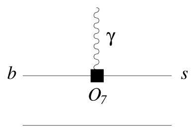
FIG. 1.:

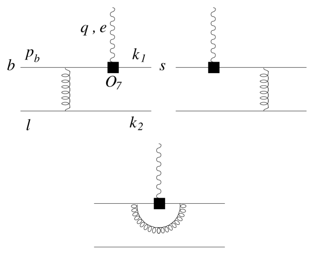
FIG. 2.:

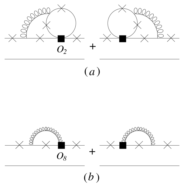
FIG. 3.:

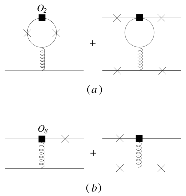
FIG. 4.:

TABLE I.: Summary of input values

$|V_{tb}V_{ts}^{*}|$	$0.0396\pm 0.0020$ [13]
$\tau_{B^{+}}$	$(1.674\pm 0.018)$ ps
$\tau_{B^{0}}$	$(1.542\pm 0.016)$ ps
$m_{B}$	5.28 GeV
$f_{B}$	0.18 GeV
$\lambda_{B}$	$(0.35\pm 0.15)$ GeV
$m_{b}(m_{b})$	4.2 GeV
$m_{c}(m_{b})$	$(1.3\pm 0.2)$ GeV

TABLE II.: $F^{A}_{+}(0)$ and $f_{A}$ from light-cone sum rules

Axial $K_{1}$	$K_{1}(1270)$	$K_{1}(1400)$
$m_{A}$	1.273 GeV	1.402 GeV
$f_{A}$	0.122 GeV	0.091 GeV
$F^{A}_{+}(0)$	$0.14\pm 0.03$	$0.098\pm 0.02$

TABLE III.: Componential contributions to the decay amplitude

$\mu_{b}$	$m_{b}(m_{b})=4.2$ GeV	$m_{b,PS}=4.6$ GeV
$C_{7}^{\rm eff(0)}(\mu_{b})$	$-0.321$	$-0.316$
$C_{7}^{\rm eff(1)}(\mu_{b})$	$0.602$	$0.522$
$C_{7}^{\rm eff}(\mu_{b})$	$-0.310$	$-0.307$
$A_{VC}(\mu_{b})$	$-0.075-i0.014$	$-0.082-i0.013$
$\mu_{H}$	$\sqrt{\Lambda_{H}m_{b}(m_{b})}=1.45$ GeV	$m_{b}(m_{b})=4.2$ GeV
$A_{HS}^{K1(1270)}(\mu_{H})$	$-0.021-i0.019$	$-0.013-i0.013$
$A_{HS}^{K1(1400)}(\mu_{H})$	$-0.022-i0.020$	$-0.014-i0.013$

TABLE IV.: Decay amplitudes and branching ratios for different scales

$(\mu_{b},\mu_{H})$ (GeV)	$(4.2,1.45)$	$(4.2,4.2)$	$(4.6,1.45)$	$(4.6,4.2)$
$(C_{7}^{\rm eff}+A_{VC}+A_{HS})_{K1(1270)}$	$-0.406-i0.033$	$-0.399-i0.027$	$-0.410-i0.033$	$-0.402-i0.026$
${\cal B}(B^{0}\to K_{1}^{0}(1270)\gamma)\times 10^{5}$	$0.828\pm 0.335$	$0.795\pm 0.329$	$0.814\pm 0.341$	$0.782\pm 0.335$
$(C_{7}^{\rm eff}+A_{VC}+A_{HS})_{K1(1400)}$	$-0.408-i0.034$	$-0.400-i0.027$	$-0.412-i0.034$	$-0.403-i0.027$
${\cal B}(B^{0}\to K_{1}^{0}(1400)\gamma)\times 10^{5}$	$0.393\pm 0.151$	$0.376\pm 0.148$	$0.386\pm 0.154$	$0.370\pm 0.150$

TABLE V.: Comparison with other results, in units of $10^{-5}$.

Branching Ratio	${\cal B}(B\to K_{1}(1270)\gamma)$	${\cal B}(B\to K_{1}(1400)\gamma)$
JPL	$0.828$	$0.393$
Ref. [24]	$0.02\sim 0.84$	$0.003\sim 0.80$
Ref. [25]	$0.493$	$0.241$
Ref. [23]	$0.45$	$0.78$
Ref. [20]	$1.20$	$0.58$
Ref. [22]	$0.3\sim 1.4$	$0.1\sim 0.6$
Ref. [19]	$1.8\sim 4.0$	$2.4\sim 5.2$
Ref. [21]	$1.1$	$0.7$