Standard Model CP violation in $B\rightarrow\,X_{d}\,\ell^{+}\ell^{-}$decays

Abstract

We investigate the CP violating asymmetry, the forward backward asymmetry and the CP violating asymmetry in the forward-backward asymmetry for the inclusive $B\rightarrow\,X_{d}\,\ell^{+}\ell^{-}$decays for the $\ell=~{}e,\,\mu,\,\tau$ channels in the standard model. It is observed that these asymmetries are quite sizable and $B\rightarrow\,X_{d}\,\ell^{+}\ell^{-}$decays seem promising for investigating CP violation.

Middle East Technical University, Physics Dept. Inonu Bul.

06531 Ankara, TURKEY

1 Introduction

An efficient way in performing the precision test for the standard model (SM) is provided by the flavor-changing neutral current (FCNC) processes since these are generated only through higher order loop effects in weak interaction. Among them, the inclusive $B\rightarrow X_{s(d)}\ell^{+}\ell^{-}$ modes are prominent because of their relative cleanness compared to the pure hadronic decays. In the SM, $B\rightarrow X_{s(d)}\ell^{+}\ell^{-}$ decays are dominated by the parton level processes $b\rightarrow s(d)\ell^{+}\ell^{-}$, which occur through an intermediate $u$, $c$ or $t$ quarks. They can be described in term of an effective Hamiltonian which contains the information about the short and long distance effects.

The FCNC decays are also relevant to the CKM phenomenology; and $b\rightarrow d\ell^{+}\ell^{-}$ modes are especially important in this respect. In case of the $b\rightarrow s\ell^{+}\ell^{-}$ decays, the matrix element receives a combination of various contributions from the intermediate $t$, $c$ or $u$ quarks with factors $V_{tb}V^{*}_{ts}\sim\lambda^{2}$, $V_{cb}V^{*}_{cs}\sim\lambda^{2}$ and $V_{ub}V^{*}_{us}\sim\lambda^{4}$, respectively, where $\lambda=\sin\theta_{C}\cong 0.22$. Since the last factor is extremely small compared to the other two we can neglect it and this reduces the unitarity relation for the CKM factors to the form $V_{tb}V^{*}_{ts}+V_{cb}V^{*}_{cs}\approx 0$. Hence, the matrix element for the $b\rightarrow s\ell^{+}\ell^{-}$ decays involve only one independent CKM factor so that CP violation would not show up. On the other hand, as pointed out before [1, 2], for $b\rightarrow d\ell^{+}\ell^{-}$ decay, all the CKM factors $V_{tb}V^{*}_{td}$, $V_{cb}V^{*}_{cd}$ and $V_{ub}V^{*}_{ud}$ are at the same order $\lambda^{3}$ in the SM and the matrix element for these processes would have sizable interference terms, so as to induce a CP violating asymmetry between the decay rates of the reactions $b\rightarrow d\ell^{+}\ell^{-}$ and $\bar{b}\rightarrow\bar{d}\ell^{+}\ell^{-}$. Therefore, $b\rightarrow d\ell^{+}\ell^{-}$ decays seem to be suitable for establishing CP violation in B mesons.

We note that the inclusive $B\rightarrow X_{s}\ell^{+}\ell^{-}$ decays have been widely studied in the framework of the SM and its various extensions [3]-[19]. As for $B\rightarrow X_{d}\ell^{+}\ell^{-}$ modes, they were first considered within the SM in [1] and [2]. In ref. [1], together with the branching ratio, the CP violating asymmetry for the $B\rightarrow\,X_{d}\,\ell^{+}\ell^{-}$decays has been studied including the long-distance (LD) effects, but only for $\ell=e$ mode. In [2], a SM analysis for the forward-backward asymmetry is given again only for $\ell=e$ mode and neglecting the LD contributions. The general two Higgs doublet model contributions and minimal supersymmetric extension of the SM (MSSM) to the CP asymmetries were discussed in refs. [20] and [21], respectively. Ref. [21] contains a comparative study of the CP asymmetries in the inclusive $B\rightarrow\,X_{d}\,\ell^{+}\ell^{-}$and exclusive $B\rightarrow\,\gamma\,\ell^{+}\ell^{-}$ decays for $\ell=\tau$ only, by mainly focusing on the effects of the scalar interactions in the framework of the MSSM. Recently, CP violation in the polarized $b\rightarrow d\ell^{+}\ell^{-}$ decay has been also investigated in the SM [22] and also in a general model independent way [23]. The aim of this work is to perform a quantitative analysis on the SM CP violation and the related observables, such as the forward-backward asymmetry and CP violation aysmmetry in the forward-backward asymmetry in the $B\rightarrow X_{d}\ell^{+}\ell^{-}$ decays, some of which have already addressed in refs. [1], [2] and [21], as pointed out above. However, in this work we extend the investigation of the abovemensioned observables to consider all three lepton modes by mainly focusing on LD effects and also their dependence on the SM parameters $\rho$ and $\eta$.

From the experimental side, the branching ratio $(BR)$ of the $B\rightarrow X_{s}\ell^{+}\ell^{-}$ decay has been also reported by the BELLE Collaboration [24], $BR(B\rightarrow X_{s}\ell^{+}\ell^{-})=((6.1\pm 1.4)^{+1.4}_{-1.1})$, which is very close to the value predicted by the SM [25], and may be used to put further constraint on the models beyond the SM.

We organized the paper as follows: Following this brief introduction, in section 2, we first present the effective Hamiltonian. Then, we introduce the basic formulas of the double and differential decay rates, CP violation asymmetry, $A_{CP}$, forward-backward asymmetry, $A_{FB}$, and CP violating asymmetry in forward-backward asymmetry $A_{CP}(A_{FB})$ for $B\rightarrow\,X_{d}\,\ell^{+}\ell^{-}$decay. Section 3 is devoted to the numerical analysis and discussion.

2 The theoretical framework of $B\rightarrow X_{d}\ell^{+}\ell^{-}$ decays

Inclusive decay rates of the heavy hadrons can be calculated in the heavy quark effective theory (HQET) [26] and the important result from this procedure is that the leading terms in $1/m_{q}$ expansion turn out to be the decay of a free quark, which can be calculated in the perturbative QCD; while the corrections to the partonic decay rate start with $1/m^{2}_{q}$ only. On the other hand, the powerful framework for both the inclusive and the exclusive modes into which the perturbative QCD corrections to the physical decay amplitude are incorporated in a systematic way is the effective Hamiltonian method. In this approach, heavy degrees of freedom, namely $t$ quark and $W^{\pm}$ bosons in the present case, are integrated out. The procedure is to take into account the QCD corrections through matching the full theory with the effective low energy one at the high scale $\mu=m_{W}$ and evaluating the Wilson coefficients from $m_{W}$ down to the lower scale $\mu\sim{\cal O}(m_{b})$. The effective Hamiltonian obtained in this way for the process $b\rightarrow d\,\ell^{+}\ell^{-}$, is given by [14], [27]-[30]:

$${\cal H}_{eff}=\frac{4G_{F}}{\sqrt{2}}\,V_{tb}V^{*}_{td}\Bigg{\{}\sum_{i=1}^{10} \,C_{i}(\mu)\,O_{i}(\mu)-\lambda_{u}\{C_{1}(\mu)[O_{1}^{u}(\mu)-O_{1}(\mu)]$$ (1)

$$+C_{2}(\mu)[O_{2}^{u}(\mu)-O_{2}(\mu)]\}\Bigg{\}}$$

where

$$\lambda_{u}=\frac{V_{ub}V_{ud}^{\ast}}{V_{tb}V_{td}^{\ast}},$$ (2)

using the unitarity of the CKM matrix i.e. $V_{tb}V_{td}^{\ast}+V_{ub}V_{ud}^{\ast}=-V_{cb}V_{cd}^{\ast}$. The explicit forms of the operators $O_{i}$ can be found in refs. [27, 28]. In Eq.(1), $C_{i}(\mu)$ are the Wilson coefficients calculated at a renormalization point $\mu$ and their evolution from the higher scale $\mu=m_{W}$ down to the low-energy scale $\mu=m_{b}$ is described by the renormalization group equation. For $C^{eff}_{7}(\mu)$ this calculation is performed in refs.[31, 32] in next to leading order. The value of $C_{10}(m_{b})$ to the leading logarithmic approximation can be found e.g. in [27, 30]. We here present the expression for $C_{9}(\mu)$ which contains the terms responsible for the CP violation in $B\rightarrow\,X_{d}\,\ell^{+}\ell^{-}$decay. It has a perturbative part and a part coming from long distance (LD) effects due to conversion of the real $\bar{c}c$ into lepton pair $\ell^{+}\ell^{-}$:

$$C_{9}^{eff}(\mu)=C_{9}^{pert}(\mu)+Y_{reson}(s)\,\,,$$ (3)

where

$$C_{9}^{pert}(\mu) = C_{9}+h(u,s)[3C_{1}(\mu)+C_{2}(\mu)+3C_{3}(\mu)+C_{4}(\mu)+3C_{5}(\mu)+C_{6}(\mu)$$

$$+ \lambda_{u}(3C_{1}+C_{2})]-\frac{1}{2}h(1,s)\left(4C_{3}(\mu)+4C_{4}(\mu)+3C_{5}(\mu)+C_{6}(\mu)\right)$$

$$- \frac{1}{2}h(0,s)\left[C_{3}(\mu)+3C_{4}(\mu)+\lambda_{u}(6C_{1}(\mu)+2C_{2}(\mu))\right]$$

$$+ \frac{2}{9}\left(3C_{3}(\mu)+C_{4}(\mu)+3C_{5}(\mu)+C_{6}(\mu)\right)\,\,,$$

and

$$Y_{reson}(s) = -\frac{3}{\alpha^{2}}\kappa\sum_{V_{i}=\psi_{i}}\frac{\pi\Gamma(V_{i}\rightarrow\ell^{+}\ell^{-})m_{V_{i}}}{m_{B}^{2}s-m_{V_{i}}+im_{V_{i}}\Gamma_{V_{i}}}$$ (5)

$$\times [(3C_{1}(\mu)+C_{2}(\mu)+3C_{3}(\mu)+C_{4}(\mu)+3C_{5}(\mu)+C_{6}(\mu))$$

$$+ \lambda_{u}(3C_{1}(\mu)+C_{2}(\mu))]\,.$$

In Eq.(2), $s=q^{2}/m_{B}^{2}$ where $q$ is the momentum transfer, $u=\frac{m_{c}}{m_{b}}$ and the functions $h(u,s)$ arise from one loop contributions of the four-quark operators $O_{1}-O_{6}$ and are given by

$$h(u,s) = -\frac{8}{9}\ln\frac{m_{b}}{\mu}-\frac{8}{9}\ln u+\frac{8}{27}+\frac{4}{9}y$$ (8)

$$-\frac{2}{9}(2+y)|1-y|^{1/2}\left\{\begin{array}[]{ll}\left(\ln\left|\frac{\sqrt{1-y}+1}{\sqrt{1-y}-1}\right|-i\pi\right),&\mbox{for }y\equiv\frac{4u^{2}}{s}<1\\ 2\arctan\frac{1}{\sqrt{y-1}},&\mbox{for }y\equiv\frac{4u^{2}}{s}>1,\end{array}\right.$$

$$h(0,s) = \frac{8}{27}-\frac{8}{9}\ln\frac{m_{b}}{\mu}-\frac{4}{9}\ln s+\frac{4}{9}i\pi\,\,.$$ (9)

The phenomenological parameter $\kappa$ in Eq. (5) is taken as $2.3$ (see e.g. [33]).

The next step is to calculate the matrix element of the $B\rightarrow X_{d}\ell^{+}\ell^{-}$ decay. Neglecting the mass of the $d$ quark, the effective short distance Hamiltonian in Eq.(1) leads to the following QCD corrected matrix element:

$${\cal M} = \frac{G_{F}\alpha}{2\sqrt{2}\pi}V_{tb}V_{td}^{\ast}\Bigg{\{}C_{9}^{eff}(m_{b})~{}\bar{d}\gamma_{\mu}(1-\gamma_{5})b\,\bar{\ell}\gamma^{\mu}\ell+C_{10}(m_{b})~{}\bar{d}\gamma_{\mu}(1-\gamma_{5})b\,\bar{\ell}\gamma^{\mu}\gamma_{5}\ell$$ (10)

$$- 2C_{7}^{eff}(m_{b})~{}\frac{m_{b}}{q^{2}}\bar{d}i\sigma_{\mu\nu}q^{\nu}(1+\gamma_{5})b\,\bar{\ell}\gamma^{\mu}\ell\Bigg{\}}.$$

Since the initial and final state polarizations are not measured, we must average over the initial spins and sum over the final ones, that leads to the following double differential decay rate

$$\frac{d^{2}\Gamma}{ds\,dz} = \Gamma(B\to X_{c}\ell\nu)\frac{\alpha^{2}}{4\pi^{2}f(u)k(u)}(1-s)^{2}\frac{|V_{tb}V^{\ast}_{td}|^{2}}{|V_{cb}|^{2}}\,v\,\Big{\{}12\,v\,z\,\mbox{\rm Re}(C^{eff}_{7}C^{*}_{10})$$ (11)

$$+ 12\,\Big{(}1+\frac{2t}{s}\Big{)}\,\mbox{\rm Re}(C^{eff}_{7}C^{eff\,*}_{9})+6\,v\,\mbox{\rm Re}(C_{10}C^{eff\,*}_{9})$$

$$+ \frac{3}{2}\Big{[}(1+s)-(1-s)\,v^{2}z^{2}+4t\Big{]}|C^{eff}_{9}|^{2}$$

$$+ 6\,\Big{[}\Big{(}1+\frac{1}{s}\Big{)}-\Big{(}1-\frac{1}{s}\Big{)}\,v^{2}z^{2}+\frac{4t}{s}\Big{]}|C^{eff}_{7}|^{2}$$

$$+ \frac{3}{2}\Big{[}(1+s)-(1-s)\,v^{2}z^{2}-4t\Big{]}|C_{10}|^{2}\Big{\}}$$

where $v=\sqrt{1-4t/s}$, $t=m^{2}_{\ell}/m^{2}_{b}$ and $z=\cos\theta$, where $\theta$ is the angle between the momentum of the B-meson and that of $\ell^{-}$ in the center of mass frame of the dileptons $\ell^{-}\ell^{+}$. In Eq. (11),

$$\Gamma(B\to X_{c}\ell\nu)=\frac{G_{F}^{2}m_{b}^{5}}{192\pi^{3}}|V_{cb}|^{2}f(u)k(u)\,,$$ (12)

where

$$f(u) = 1-8u+8u^{4}-u^{8}-24u^{4}ln(u)$$ (13)

$$k(u) = 1-\frac{2\alpha_{s}(m_{b})}{3\pi}\Bigg{[}\left(\pi^{2}-\frac{31}{4}\right)(1-\hat{m}_{c}^{2})+{3\over 2}\Bigg{]}\,,$$ (14)

are the phase space factor and the QCD corrections to the semi-leptonic decay rate, respectively, which is used to normalize the decay rate of $B\rightarrow X_{d}\ell^{+}\ell^{-}$ to remove the uncertainties in the value of $m_{b}$.

After integrating the double differential decay rate in Eq.(11) over the angle variable, we find

$$\frac{d\Gamma}{ds}=\Gamma(B\to X_{c}\ell\nu)\frac{\alpha^{2}}{4\pi^{2}f(u)k(u)}(1-s)^{2}\frac{|V_{tb}V^{\ast}_{td}|^{2}}{|V_{cb}|^{2}}\sqrt{1-\frac{4t}{s}}\,\Delta(s)\,,$$ (15)

where

$$\Delta(s) = \frac{(s+2s^{2}+2t-8st)}{s}|C_{10}|^{2}+\frac{4}{s^{2}}(2+s)(s+2t)|C^{eff}_{7}|^{2}+(2+s)(1+\frac{2t}{s})|C^{eff}_{9}|^{2}$$ (16)

$$+ \frac{12}{s}(s+2t)\mbox{\rm Re}(C^{eff}_{7}C^{eff\,*}_{9})\,.$$

We start with calculating the CP asymmetry $A_{CP}$ between the $B\rightarrow X_{d}\ell^{+}\ell^{-}$ and the conjugated one $\bar{B}\rightarrow\bar{X_{d}}\ell^{+}\ell^{-}$, which is defined as

$$A_{CP}(s)~{}=~{}\frac{\frac{d\Gamma}{ds}-\frac{d\bar{\Gamma}}{ds}}{\frac{d\Gamma}{ds}+\frac{d\bar{\Gamma}}{ds}}$$ (17)

where

$$\frac{d\Gamma}{ds}~{}=~{}\frac{d\Gamma(B\rightarrow X_{d}\ell^{+}\ell^{-})}{ds}~{}~{},~{}~{}\frac{d\bar{\Gamma}}{ds}~{}=~{}\frac{d\Gamma(\bar{B}\rightarrow\bar{X_{d}}\ell^{+}\ell^{-})}{ds}\,.$$ (18)

Since in the SM only $C^{eff}_{9}$ contains imaginary part, representing $C^{eff}_{9}$ symbolically as

$$C^{eff}_{9}~{}=~{}\xi_{1}+\lambda_{u}\xi_{2}$$ (19)

and further substituting $\lambda\rightarrow\lambda^{\ast}$ for the conjugated process $\bar{B}\rightarrow\bar{X_{d}}\ell^{+}\ell^{-}$, one can easily obtain [1]

$$A_{CP}(s) = \frac{-2\,\mbox{\rm Im}(\lambda_{u})\,\Sigma}{\Delta+2\,\mbox{\rm Im}(\lambda_{u})\,\Sigma}\,,$$ (20)

where

$$\Sigma = \Big{(}1+\frac{2t}{s}\Big{)}[(1+2s)\,\mbox{\rm Im}(\xi^{\ast}_{1}\xi_{2})+6\,C^{eff}_{7}\,\mbox{\rm Im}(\xi_{2})]\,\mbox{\rm Im}(\lambda_{u})\,.$$ (21)

For completeness, we next consider the forward-backward asymmetry, $A_{FB}$, in $B\rightarrow\,X_{d}\,\ell^{+}\ell^{-}$, which is another physical quantity that may be useful to test the theoretical models. Using the definition of differential $A_{FB}(s)$

$$A_{FB}(s) = \frac{\int^{1}_{0}dz\frac{d^{2}\Gamma}{dsdz}-\int^{0}_{-1}dz\frac{d^{2}\Gamma}{dsdz}}{\int^{1}_{0}dz\frac{d^{2}\Gamma}{dsdz}+\int^{0}_{-1}dz\frac{d^{2}\Gamma}{dsdz}}\,,$$ (22)

we find

$$A_{FB}(s)=\frac{3~{}v}{\Delta(s)}\,\mbox{\rm Re}[C_{10}(2C^{eff}_{7}+s\,C^{eff\,*}_{9})],$$ (23)

which agrees with the result given by ref. [2], but not by [21].

We have also a CP violating asymmetry in $A_{FB}$, $A_{CP}(A_{FB})$, in $B\rightarrow\,X_{d}\,\ell^{+}\ell^{-}$decay. Since in the limit of CP conservation, one expects $A_{FB}=-\bar{A}_{FB}$ [2, 34], where $A_{FB}$ and $\bar{A}_{FB}$ are the forward-backward asymmetries in the particle and antiparticle channels, respectively, $A_{CP}(A_{FB})$ is defined as

$$A_{CP}(A_{FB}) = A_{FB}+\bar{A}_{FB}~{}~{}.$$ (24)

Here, $\bar{A}_{FB}$ can be obtained by the replacement,

$$C_{9}^{eff}(\lambda_{u})\rightarrow\bar{C}_{9}^{eff}(\lambda_{u}\rightarrow\lambda_{u}^{\ast}).$$ (25)

Using Eqs.(23) we can find

$$A_{CP}(A_{FB}) = \frac{6~{}v~{}\mbox{\rm Im}(\lambda_{u})}{\Delta(\Delta+4\mbox{\rm Im}(\lambda_{u})~{}\Sigma)}~{}C_{10}$$

$$\cdot \Big{[}2\Sigma~{}(2C^{eff}_{7}+s(\mbox{\rm Re}(\xi_{1})+\mbox{\rm Re}(\xi_{2})~{}\mbox{\rm Re}(\lambda_{u})-\mbox{\rm Im}(\xi_{2})~{}\mbox{\rm Im}(\lambda_{u})))-s~{}\Delta~{}\mbox{\rm Im}(\xi_{2})\Big{]}\,,$$

which is slightly different from the one given by ref. [21].

3 Numerical analysis and discussion

In this section, we present results of our calculations related to $B\rightarrow\,X_{d}\,\ell^{+}\ell^{-}$decays, for two different sets of the Wolfenstein parameters. For this we first give the Wolfenstein parametrization [35] of the CKM factor in Eq.(2)

$$\lambda_{u}=\frac{\rho(1-\rho)-\eta^{2}-i\eta}{(1-\rho)^{2}+\eta^{2}}+O(\lambda^{2})\,,$$ (27)

and also

$$\frac{|V_{tb}V^{\ast}_{td}|^{2}}{|V_{cb}|^{2}} = \lambda^{2}[(1-\rho)^{2}+\eta^{2}]+{\cal O}(\lambda^{4})\,.$$ (28)

The updated fitted values for the parameters $\rho$ and $\eta$ are given in ref.[36] as

$$\bar{\rho} = 0.22\pm 0.07\,\,(0.25\pm 0.07)$$

$$\bar{\eta} = 0.34\pm 0.04\,\,(0.34\pm 0.04)$$ (29)

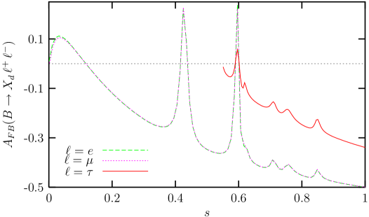
Figure 4: The same as Fig.(3) but for the Wolfenstein parameters $(\rho,\,\eta)=(0.32;\,0.38)$

with (without) including the chiral logarithms uncertainties. In our numerical analysis, we have used $(\rho,\,\eta)=(0.15;\,0.30)$ and $(0.32;\,0.38)$, which are the lower and higher allowed values of the parameters given in Eq. (29) above, and present the dependence of the $A_{CP}$, $A_{FB}$ and $A_{CP}(A_{FB})$ on the dimensionles photon energy $s$ for the $B\rightarrow\,X_{d}\,\ell^{+}\ell^{-}$$(\ell=e,\,\mu,\,\tau)$ decays in Figs. (1-6).

We have also evaluated the average values of CP asymmetry $<A_{CP}>$, forward-backward asymmetry $<A_{FB}>$ and CP asymmetry in the forward-backward asymmetry $<A_{CP}(A_{FB})>$ in $B\rightarrow\,X_{d}\,\ell^{+}\ell^{-}$decay for the above sets of parameters $(\rho,\,\eta)$, and our results are displayed in Table 1 and 2 without and with including the long distance effects, respectively.

The input parameters and the initial values of the Wilson coefficients we used in our numerical analysis are as follows:

$$m_{B}=5.28\,GeV\,,\,m_{b}=4.8\,GeV\,,\,m_{c}=1.4\,GeV\,,m_{t}=175\,GeV\,,$$

$$m_{e}=0.511\,MeV\,\,,\,\,m_{\tau}=1.777\,GeV,\,m_{\mu}=0.105\,GeV,\,,\,$$

$$BR(B\rightarrow X_{c}e\bar{\nu}_{e})=10.4\%\,\,,\,\,\alpha=1/129\,\,,\,\,m_{W}=80.4\,GeV\,\,,\,\,m_{Z}=91.1\,GeV$$

$$C_{1}=-0.245,\,C_{2}=1.107,\,C_{3}=0.011,\,C_{4}=-0.026,\,C_{5}=0.007,\,$$

$$C_{6}=-0.0314,\,C^{eff}_{7}=-0.315,\,C_{9}=4.220,\,C_{10}=-4.619.$$ (30)

In our numerical analysis, we take into account five possible resonances for the LD effects coming from the reaction $b\rightarrow d\,\psi_{i}\rightarrow d\,\ell^{+}\ell^{-}$, where $i=1,...,5$ and divide the integration region into two parts for $\ell=\tau$: $(2m_{\ell}/m_{B})^{2}\leq s\leq((m_{\psi_{1}}-0.02)/m_{B})^{2}$ and $((m_{\psi_{1}}+0.02)/m_{B})^{2}\leq s\leq 1$, where $m_{\psi_{1}}=3.097$ GeV is the mass of the first resonance. As for $\ell=e$ and $\mu$ modes, the integration region is divided into three parts : $(2m_{\ell}/m_{B})^{2}\leq s\leq((m_{\psi_{1}}-0.02)/m_{B})^{2}$, $((m_{\psi_{1}}+0.02)/m_{B})^{2}\leq s\leq((m_{\psi_{2}}-0.02)/m_{B})^{2}$ and $((m_{\psi_{2}}+0.02)/m_{B})^{2}\leq s\leq 1$, where $m_{\psi_{2}}=3.686$ GeV is the mass of the second resonance.

For reference, we present our SM predictions with long distance effects

$$BR(B\rightarrow X_{d}\,\ell^{+}\,\ell^{-}) = (3.01,2.61,0.11)\times 10^{-7}\,,$$ (31)

for $\ell=e,\mu,\tau$, respectively, with $(\rho;\eta)=(0.30;0.34)$, which is in agreement with the results of ref.[1].

		$<A_{CP}>$			$<A_{FB}>$			$<A_{CP}(A_{FB}>$)
$(\rho;\,\eta)$	$\ell~{}=~{}e$	$\ell~{}=~{}\mu$	$\ell~{}=~{}\tau$	$\ell~{}=~{}e$	$\ell~{}=~{}\mu$	$\ell~{}=~{}\tau$	$\ell~{}=~{}e$	$\ell~{}=~{}\mu$	$\ell~{}=~{}\tau$
$(0.15;\,0.30)$	$0.030$	$0.036$	$0.134$	$-0.124$	$-0.151$	$-0.182$	$-0.009$	$-0.009$	$0.001$
$(0.32;\,0.38)$	$0.051$	$0.061$	$0.169$	$-0.129$	$-0.156$	$-0.180$	$-0.015$	$-0.015$	$0.002$

Table 1: The average values of $A_{CP}$, $A_{FB}$ and $A_{CP}(A_{FB})$ in $B\rightarrow\,X_{d}\,\ell^{+}\ell^{-}$for the three distinct lepton modes without including the long distance effects.

		$<A_{CP}>$			$<A_{FB}>$			$<A_{CP}(A_{FB}>)$
$(\rho;\,\eta)$	$\ell~{}=~{}e$	$\ell~{}=~{}\mu$	$\ell~{}=~{}\tau$	$\ell~{}=~{}e$	$\ell~{}=~{}\mu$	$\ell~{}=~{}\tau$	$\ell~{}=~{}e$	$\ell~{}=~{}\mu$	$\ell~{}=~{}\tau$
$(0.15;\,0.30)$	$0.032$	$0.036$	$0.144$	$-0.119$	$-0.139$	$-0.157$	$-0.017$	$-0.017$	$-0.004$
$(0.32;\,0.38)$	$0.051$	$0.059$	$0.230$	$-0.125$	$-0.140$	$-0.150$	$-0.031$	$-0.030$	$-0.009$

Table 2: The same as Table (1), but including the long distance effects.

In Fig.(1) and Fig.(2), we present the dependence of $A_{CP}$ on the dimensionless photon energy $s$, for $B\rightarrow\,X_{d}\,\ell^{+}\ell^{-}$decay for the Wolfenstein parameters $(\rho;\,\eta)=(0.15;\,0.30)$ and $(\rho;\,\eta)=(0.32;\,0.38)$, respectively. The three distinct lepton modes $\ell=~{}e,~{}\mu,~{}\tau$ are represented by the dashed, dotted and solid curves, respectively. We observe that the $A_{CP}$ for $\ell=~{}e,~{}\mu$ cases almost coincide, reaching up to $25~{}\%$ for the larger values of $s$. The $A_{CP}$ for $\ell=~{}\tau$ mode exceeds the values of the other modes and reaches $40~{}\%$. We also observe from Tables 1 and 2 that including the LD effects in calculating $<A_{CP}>$ does not change the results for $\ell=~{}e,~{}\mu$ modes, while $\ell=~{}\tau$ mode, it is quite sizable, $8-36\%$, depending on the sets of the parameters used for $(\rho;\,\eta)$.

The $s$ dependence of $A_{FB}$ for the $B\rightarrow\,X_{d}\,\ell^{+}\ell^{-}$$(\ell=~{}e,~{}\mu,~{}\tau)$ decays are plotted in Figs.(3) and (4) for $(\rho;\,\eta)=(0.15;\,0.30)$ and $(\rho;\,\eta)=(0.32;\,0.38)$, respectively. We see that $A_{FB}$ is negative for almost all values of $s$, except in the resonance and very small-$s$ regions. $<A_{FB}>$ takes the values between $-(12-15)\%$ depending on the sets of the parameters used for $(\rho;\,\eta)$ . The LD effects on $<A_{FB}>$ are about $10\%$, but in reverse manner, decreasing its magnitude in comparison to the values without LD contributions.

We present the dependence of the $A_{CP}(A_{FB})$ of $B\rightarrow\,X_{d}\,\ell^{+}\ell^{-}$decay on $s$ in Fig.(5) and Fig.(6), again for two different sets of the Wolfenstein parameters. As for $A_{CP}$, $A_{CP}(A_{FB})$ for $\ell=~{}e,$ and $\ell=~{}\mu$ modes almost coincide. We see that $A_{CP}(A_{FB})$ is all negative except in a very small region for the intermediate values of $s$ for $\ell=~{}e,~{}\mu$ cases. LD effects seem to be quite significant for $<A_{CP}(A_{FB})>$, enhancing its value twice (four times) for $\ell=~{}e,~{}\mu$ ($\ell=~{}\tau$) modes. To see this LD contributions more closely, we present the $<A_{CP}(A_{FB})>$ for different regions of $s$ in Table (3) and (4), for $(\rho;\,\eta)=(0.15;\,0.30)$ and $(\rho;\,\eta)=(0.32;\,0.38)$, respectively. We see that for the light lepton modes, $\ell=e,\mu$, $A_{CP}(A_{FB})$ is more sizable in the high-dilepton mass region of $s$, $((m_{\psi_{2}}+0.02)/m_{B})^{2}\leq s\leq 1$. However, for $\ell=\tau$, the contribution from the high-dilepton mass region of $s$ is negligible and the contribution to $<A_{CP}(A_{FB})>$ comes effectively from the low-dilepton mass region, $(2m_{l}/m_{B})^{2}\leq s\leq((m_{\psi_{1}}-0.02)/m_{B})^{2}$ and amounts to $-1\%$.

	SD	$(2m_{l}/m_{B})^{2}\leq s\leq$	$((m_{\psi_{1}}+0.02)/m_{B})^{2}\leq s$	$((m_{\psi_{2}}+0.02)/m_{B})^{2}$	SD+LD
$\ell$	contribution	$((m_{\psi_{1}}-0.02)/m_{B})^{2}$	$\leq((m_{\psi_{2}}-0.02)/m_{B})^{2}$	$\leq s\leq 1$	contribution
e	$-0.92$	$-0.29$	$-0.25$	$-1.20$	$-1.78$
$\mu$	$-0.91$	$-0.29$	$-0.25$	$-1.20$	$-1.78$
$\tau$	$-0.11$	$-0.42$	$3.10\times 10^{-3}$		$-0.42$

Table 3: The SM predictions for the average CP-violating asymmetry in the forward-backward asymmetry $<A_{CP}(A_{FB})>\times 10^{-2}$ for different regions of the dimensionless photon energy $s$ with $(\rho;\eta)=(0.15;\,0.30)$.

	SD	$(2m_{l}/m_{B})^{2}\leq s\leq$	$((m_{\psi_{1}}+0.02)/m_{B})^{2}\leq s$	$((m_{\psi_{2}}+0.02)/m_{B})^{2}$	SD+LD
$\ell$	contribution	$((m_{\psi_{1}}-0.02)/m_{B})^{2}$	$\leq((m_{\psi_{2}}-0.02)/m_{B})^{2}$	$\leq s\leq 1$	contribution
e	$-1.59$	$-0.51$	$-0.43$	$-2.15$	$-3.10$
$\mu$	$-1.57$	$-0.51$	$-0.43$	$-2.15$	$-3.09$
$\tau$	$0.20$	$-0.94$	$3.30\times 10^{-3}$		$-0.94$

Table 4: Same as Table (3), but with $(\rho;\eta)=(0.32;\,0.38)$.

As a conclusion we can say that there is a significant $A_{CP}$ and $A_{CP}(A_{FB})$ for the $B\rightarrow\,X_{d}\,\ell^{+}\ell^{-}$decay, although the branching ratios predicted for these channels are relatively small because of CKM suppression. So, $B\rightarrow\,X_{d}\,\ell^{+}\ell^{-}$decays seem promising for investigating CP violation.

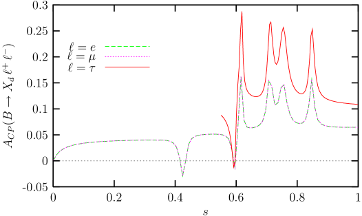
Figure 1: $A_{CP}$ for $B\rightarrow\,X_{d}\,\ell^{+}\ell^{-}$decay for the Wolfenstein parameters $(\rho,\,\eta)=(0.15;\,0.30)$. The three distinct lepton modes $\ell=~{}e,~{}\mu,~{}\tau$ are represented by the dashed, dotted and solid curves, respectively.

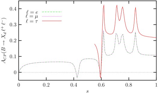
Figure 2: The same as Fig.(1) but for the Wolfenstein parameters $(\rho,\,\eta)=(0.32;\,0.38)$

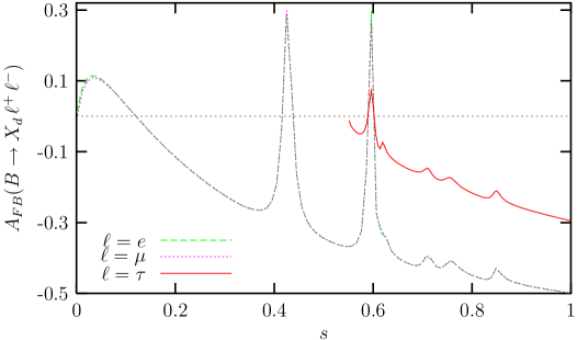
Figure 3: $A_{FB}$ for $B\rightarrow\,X_{d}\,\ell^{+}\ell^{-}$decay for the Wolfenstein parameters $(\rho,\,\eta)=(0.15;\,0.30)$. The three distinct lepton modes $\ell=~{}e,~{}\mu,~{}\tau$ are represented by the dashed, dotted and solid curves, respectively.

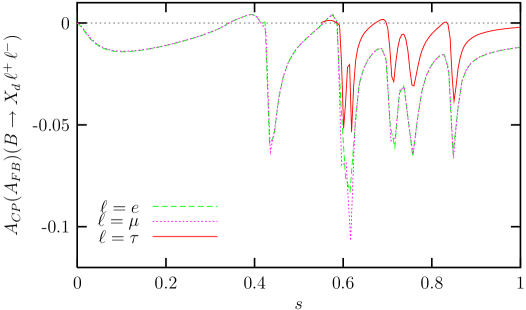
Figure 5: $A_{CP}(A_{FB})$ for $B\rightarrow\,X_{d}\,\ell^{+}\ell^{-}$decay for the Wolfenstein parameters $(\rho,\,\eta)=(0.15;\,0.30)$. The three distinct lepton modes $\ell=~{}e,~{}\mu,~{}\tau$ are represented by the dashed, dotted and solid curves, respectively.

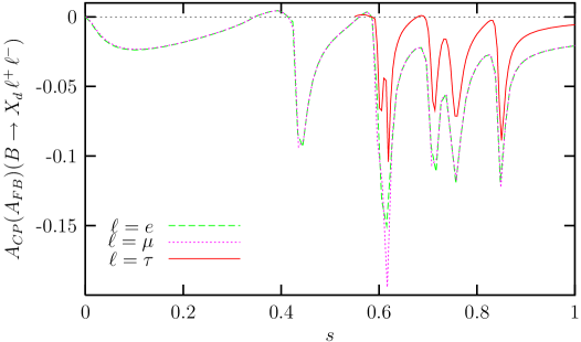
Figure 6: The same as Fig.(5) but for the Wolfenstein parameters $(\rho,\,\eta)=(0.32;\,0.38)$

References

[1] F. Krüger, L.M. Sehgal, Phys. Rev., D55, (1997) 2799.
[2] S. Rai Choudhury, Phys. Rev., D56, (1997) 6028.
[3] W. S. Hou, R. S. Willey and A. Soni,
Phys. Rev. Lett.58 (1987) 1608.
[4] N. G. Deshpande and J. Trampetic,
Phys. Rev. Lett.60 (1988) 2583.
[5] C. S. Lim, T. Morozumi and A. I. Sanda,
Phys. Lett.B218 (1989) 343.
[6] B. Grinstein, M. J. Savage and M. B. Wise,
Nucl. Phys.B319 (1989) 271.
[7] C. Dominguez, N. Paver and Riazuddin,
Phys. Lett.B214 (1988) 459.
[8] N. G. Deshpande, J. Trampetic and K. Ponose,
Phys. Rev.D39 (1989) 1461.
[9] P. J. O’Donnell and H. K. Tung,
Phys. Rev.D43 (1991) 2067.
[10] N. Paver and Riazuddin,
Phys. Rev.D45 (1992) 978.
[11] A. Ali, T. Mannel and T. Morozumi,
Phys. Lett.B273 (1991) 505.
[12] A. Ali, G. F. Giudice and T. Mannel,
Z. Phys.C67 (1995) 417.
[13] C. Greub, A. Ioannissian and D. Wyler,
Phys. Lett.B346 (1995) 145;
D. Liu Phys. Lett.B346 (1995) 355;
G. Burdman, Phys. Rev.D52 (1995) 6400:
Y. Okada, Y. Shimizu and M. Tanaka Phys. Lett.B405
(1997) 297.
[14] A. J. Buras and M. Münz,
Phys. Rev.D52 (1995) 186.
[15] N. G. Deshpande, X. -G. He and J. Trampetic,
Phys. Lett.B367 (1996) 362.
[16] W. Jaus and D. Wyler,
Phys. Rev.D41 (1990) 3405.
[17] Y. B. Dai, C. S. Huang and H. W. Huang,
Phys. Lett.B390 (1997) 257,
C. S. Huang, L. Wei,
Q. S. Yan and S. H. Zhu, Phys. Rev.D63 (2001) 114021.
[18] H. E. Logan and U. Nierste, Nucl. Phys.B586
(2000) 39.
[19] E. Iltan and G. Turan,
Phys. Rev.D63 (2001) 115007.
[20] T. M. Aliev and M.Savcı, Phys. Lett.B 452 (1999) 318.
[21] S. Rai Choudhury and N. Gaur, hep-ph/0207353.
[22] K. S. Babu, K. R. S. Balaji and I. Schienbein,Phys. Rev., D68, (2003) 014021.
[23] T. M. Aliev, V. Bashiry, and M. Savcı, hep-ph/0308069.
[24] J. Kaneko et al., BELLE Collaboration, Phys. Rev. Lett., 90, (2003) 021801.
[25] A. Ali, E. Lunghi, C. Greub and G. Hiller, Phys. Rev., D66, (2002) 034002.
[26]For a review, see, M. Neubert, Phys. Rep., 245, (1994) 396.
[27] G. Buchalla, A. Buras, and M. Lautenbacher, Rev. Mod. Phys., 68 (1996) 1125.
[28] B. Grinstein, R. Springer, and M. Wise, Nucl. Phys., B339 (1990) 269.
[29] A. J. Buras, M. Misiak, M. Münz, and S. Pokorski,
Nucl. Phys.B 424 (1994) 372.
[30] M. Misiak,
Nucl. Phys.B 393 (1993) 23; B 439 (1993) 461 (E).
[31] F. Borzumati and C. Greub,
Phys. Rev.D 58 (1998) 074004.
[32] M. Ciuchini, G. Degrassi, P. Gambino, and G. F. Giudice,
Nucl. Phys.B 527 (1998) 21.
[33] Z. Ligeti, I. W. Stewart, M. B. Wise Phys.Lett.B420 (1998) 359.
[34] G. Buchalla, G. Hiller and G. Isidori,
Phys. Rev.D 63 (2000) 014015.
[35] L. Wolfenstein,
Phys. Rev. Lett.51 (1983) 1945.
[36] A. Ali, and E. Lunghi,
Eur. Phys. J.C 26 (2002) 195.