CERN-PH-TH/2004-036 IFT-2004-08

We discuss the stabilization of the scalar sector, including the radion, in the gauge model with one universal extra dimension, within Higgs and Higgsless scenarios. The stabilization occurs at the one-loop level, through the fermionic contribution to the effective potential; in the Higgs case, for stabilization to take place the bosonic contribution must be balanced by the fermionic one, hence the scales of these two cannot differ too much. However, there is no need for (softly broken) supersymmetry to achieve the stabilization - it can be arranged for a reasonably wide range of couplings and mass scales. The primary instability in the model is the run-away of the radion vacuum expectation value. It turns out that the requirement of the radion stability, in the Higgs case, favours a Higgs boson mass below $0.26$ TeV, which is consistent with the Standard Model upper bound that follows from the electroweak precision measurements. The typical radion mass is of the order of $\sim 10^{-6}$ eV. The radion mass can be made larger by rising the scale of fermion masses, as clearly seen in the Higgsless case. The cosmological constant may be cancelled by suitable counterterms, in such a way that the stabilization is not affected.

PACS: 04.50.+h, 12.60.Fr

Keywords: extra dimensions, radion, stabilization, gauge symmetry breaking

1 Introduction

Understanding the origin of the electroweak symmetry breaking at $M_{EWB}\leq 1$ TeV and the fermion mass generation appears to be one of the big theoretical challenges of contemporary physics. There exist various ideas of how to give mass to the gauge bosons mediating weak interactions and how to, simultaneously, render the scale of the breaking in the $1$ TeV range in the presence of radiative corrections. One of the most natural tools is supersymmetry, another one - extra dimensions, which offer new possibilities both for electroweak breaking and for supersymmetry breaking (e.g. by suitable boundary conditions). However, with extra dimensions there appears a new issue in the game - the problem of stabilization of compact dimensions, which, in fact, seems to be a disguised version of the familiar, well-known hierarchy problem. In this note we would like to address, in the simplest possible set-up, the question of the interrelation between these issues. About the supersymmetry breaking we shall be rather brief here, simply assuming that it is somehow broken, perhaps even in a hard way; hence, for instance, the number of fermions does not need to match the number of bosons in the model. Taking that for granted, we consider here one-loop corrections to the effective potential for the radion (which is the scalar excitation of the extra-dimensional metric tensor whose vacuum expectation value fixes the size of extra dimensions) and the Higgs boson, as a source of the radion stabilization. It turns out that it is possible to create a non-trivial and quasi-realistic minimum of the effective potential in the space spanned by the scalar fields of the theory, with one universal extra dimension in two cases of special interest. Firstly, when the electroweak breaking is caused by the condensation of the higher-dimensional Higgs scalar, and secondly in the Higgsless case, when we imagine that the massless mode of gauge fields is removed from the spectrum by boundary conditions. The notorious feature of the set-up containing a Higgs boson is a light, in fact too light, radion excitation. In the Higgsless case it is much easier to avoid such a problem: it is possible to raise the radion mass by coupling a radion to heavy fermions living in the bulk of the model. We find it amusing and encouraging at the same time to find stable vacuum states with stable extra dimensions and broken gauge symmetry with essentially arbitrarily broken supersymmetry.

The paper is organized as follows. In Section 2 we define the 5d Higgs model. Section 3 contains details of the reduction from 5d to 4d. In Section 4 we calculate the one-loop effective potential in order to determine the radion mass and we comment on the existing experimental constraints on the radion mass. Section 5 is devoted to the discussion of the radion stability in the Higgsless scenario. Summary and comment on consequences of possible variations of the set-up adopted here are presented in Section 6. The appendix contains details of the derivation of the effective potential.

2 General set-up

Let us start with the following action in 5d

$$S=S_{g}+S_{s}+S_{f}+S_{v}+S_{gf}\,,$$ (1)

where $S_{g}$ denotes the Einstein–Hilbert action,

$$S_{g}=-\frac{1}{2}M_{5}^{3}\int_{0}^{L}dy\int d^{4}x\sqrt{G}R^{(5)}\,,$$ (2)

where $R^{(5)}$ is the Ricci scalar constructed from the 5d metric tensor $G_{MN}$ and $L=2\pi\rho$. The scale $M_{5}$ sets the 5d gravitational coupling. The notation for the Lorentz indices and space-time coordinates is as follows: $M,N=0,1,2,3,5$; $\mu,\nu=0,1,2,3$ and $y=x^{5}$ is the coordinate of the extra dimension. The action for the complex scalar field and vector bosons reads

$$S_{s} = \int_{0}^{L}dy\int d^{4}x\sqrt{G}\left[(D_{M}\phi)^{*}(D^{M}\phi)-V^{(5)}(\phi)\right]\,,$$ (3)

$$S_{v}+S_{gf} = \int_{0}^{L}dy\int d^{4}x\sqrt{G}\left\{-\frac{1}{4}F^{MN}F_{MN}-\frac{1}{2\xi}\left[\partial_{\mu}A^{\mu}-\xi\left(\partial_{5}A_{5}+ev\chi\right)\right]^{2}\right\}\,,$$ (4)

where $v$ is the vacuum expectation value of the zero mode of the scalar field, $e_{4}\equiv e_{5}/\sqrt{L}$ will appear to be the effective 4d electromagnetic gauge coupling and

$$F_{MN}=\partial_{M}A_{N}-\partial_{N}A_{M}\,, D_{M}=\partial_{M}+{\rm i}e_{5}A_{M}\,,$$

$$V^{(5)}(\phi)=\lambda_{5}\left(|\phi|^{2}-\frac{\mu^{2}}{2\lambda_{5}}\right)^{2}\,, \phi=\frac{1}{\sqrt{2}}\left(h+{\rm i}\chi\right)\,.$$

Here we will adopt the Landau gauge, which is equivalent to the limit $\xi\to 0$.

In order to construct a Standard Model-like theory, we will follow Ref. [1] and introduce two fermionic fields $\psi=\psi(x,y)$ (charged) and $\lambda=\lambda(x,y)$ (neutral) with the following transformation properties:

$$\psi(x,y)\to\gamma_{5}\psi(x,L-y)\;\;\;\;\;\;{\rm and}\;\;\;\;\;\;\lambda(x,y)\to-\gamma_{5}\lambda(x,L-y)\,,$$ (5)

while for the bosonic fields we assume

$$\phi(x,y)\to\phi(x,L-y),\;\;A_{\mu}(x,y)\to A_{\mu}(x,L-y)\;\;{\rm and}\;\;A_{5}(x,y)\to-A_{5}(x,L-y)\,.$$ (6)

Then, the invariant fermionic action reads:

$$S_{f}=\int_{0}^{L}dy\int d^{4}x\sqrt{G}\left[{\rm i}\overline{\psi}\gamma^{M}(\partial_{M}+{\rm i}e_{5}A_{M})\psi+{\rm i}\overline{\lambda}\gamma^{M}\partial_{M}\lambda-\left(g_{5}\overline{\psi}\phi\lambda+\hbox{H.c.}\right)\right]\,,$$ (7)

As can be seen, the fermion mass term is generated (as in the Standard Model (SM)) by the scalar vacuum expectation value.

The size of the extra dimension $L=2\pi\rho$ is an arbitrary parameter with the dimension of length. It has no physical meaning. What is physically meaningful is the distance along the compact dimension

$$L_{\rm phys}=\int_{0}^{L}dx^{5}\sqrt{-G_{55}}\,.$$ (8)

3 Compactification

Let us construct the 4d effective theory. Since hereafter we will consider neither Kaluza–Klein (KK) modes of the 4d metric $g_{\mu\nu}(x,y)$ nor those of the radion $R_{0}(x,y)$, the background 5d metric can be parametrized as

$$G_{MN}=\left(\begin{array}[]{cc}g_{\mu\nu}(x)&0\\ 0&-R_{0}^{2}(x)\end{array}\right)\,.$$ (9)

The compactification of the extra dimension is specified by the following $S^{1}/Z_{2}$ orbifold conditions:

$$A_{\mu}(x,y)=A_{\mu}(x,-y)\,,\;\;\; A_{5}(x,y)=-A_{5}(x,-y)\,,$$

$$\phi(x,y)=\phi(x,-y)\,,$$

$$\psi_{R}(x,y)=\psi_{R}(x,-y)\,,\;\;\; \psi_{L}(x,y)=-\psi_{L}(x,-y)\,,$$

$$\lambda_{L}(x,y)=\lambda_{L}(x,-y)\,,\;\;\; \lambda_{R}(x,y)=-\lambda_{R}(x,-y)\,.$$

Moreover, the fields should remain unchanged under the shift $y\rightarrow y+2\pi\rho$. The resulting KK expansion is given in the appendix.

An important remark is in order here. In general, instead of discussing the circle and its symmetries, one could go immediately to a line segment and impose boundary conditions on the fields by coupling them to suitable sources localized on the branes. These sources appear in the equations of motion and enforce a definite behaviour of the fields at the boundaries. This way one may obtain boundary conditions corresponding to fields living on a quarter of a circle, or on $S^{1}/Z_{2}\times Z^{{}^{\prime}}_{2}$. It is often convenient to discuss such set-ups on a circle; however one then has to accept fields that are not periodic. We shall discuss such a case later in the paper.

After integrating out the extra coordinate, we find the effective Einstein–Hilbert term multiplied by a a power of the radion field

$$S_{g}^{\rm eff}=-\frac{1}{2}M_{5}^{3}2\pi\rho\int d^{4}x\sqrt{-g}|R_{0}|R^{(4)}\,.$$ (10)

It will be useful to transform the above action to the Einstein frame by performing the following Weyl rescaling

$$g_{\mu\nu}\longrightarrow|R_{0}|^{-1}g_{\mu\nu}\,,$$ (11)

which results in the gravitational action

$$S_{g}^{\rm eff}=-\frac{1}{2}M_{4}^{2}\int d^{4}x\sqrt{-g}R^{(4)}+\frac{1}{2}\int d^{4}x\sqrt{-g}\partial_{\mu}r\partial^{\mu}r\,,$$ (12)

where we have defined $r=\sqrt{3/2}M_{4}\log{|R_{0}|}$, and $M_{4}$ denotes the effective 4d Planck scale. It is worth emphasizing that the Weyl rescaling is essential here; it is necessary to properly identify the 4d metric as the one that appears on the r.h.s. of Eq. (11), for which we obtain the canonical form of the Einstein gravity action in Eq. (12). Notice also that our definition $M_{4}^{2}=2\pi\rho M_{5}^{3}$ does not express a relation between four- and five-dimensional Planck scales. Precise analysis of the Newton law shows that the actual 5d Planck scale, related to the 5d Newton constant, reads $M_{5}^{\rm true}=M_{5}\langle|R_{0}|\rangle^{-1/3}$, and then $M_{4}^{2}=2\pi\rho\langle|R_{0}|\rangle(M_{5}^{\rm true})^{3}$.

It is straightforward to verify that, after the Weyl rescaling, we must also rescale $A_{\mu}$ and $A_{5}$ to obtain canonical kinetic action

$$A_{\mu}\longrightarrow|R_{0}|^{-\frac{1}{2}}A_{\mu}\,,\quad A_{5}\longrightarrow|R_{0}|A_{5}\,.$$ (13)

The following redefinition is necessary for fermionic fields as well

$$\psi\longrightarrow|R_{0}|^{\frac{1}{4}}\psi\,,\quad\lambda\longrightarrow|R_{0}|^{\frac{1}{4}}\lambda\,.$$ (14)

After the Weyl rescaling the 5d metric takes the following form

$$ds^{2}=R_{0}^{-1}g_{\mu\nu}dx^{\mu}dx^{\nu}-R_{0}^{2}dy^{2}\,.$$ (15)

Hence, the physical size of the extra dimension is given by $L_{\rm phys}=2\pi\rho\langle R_{0}\rangle$, where $\langle R_{0}\rangle$ is determined by the quantum corrections computed by expanding the Lagrangian around the classical solution of the 5d Einstein equations

$$\begin{array}[]{c}g_{\mu\nu}=\eta_{\mu\nu}\\ \\ R_{0}(x)=\langle R_{0}\rangle={\rm const.}\,,\end{array}$$ (16)

$\eta_{\mu\nu}$ being the Minkowski metric.

It should be noted that the rescaling (13) and (14) generates a number of derivative-type couplings of the radion. Those, however, are not relevant to the calculation of the one-loop effective potential and therefore will not longer be considered.

4 Radiative corrections

After the Weyl rescaling, the 4d tree-level potential in the Landau gauge is obtained, as the following integral over the extra dimension:

$$V^{4}(\phi,r)=\int_{0}^{2\pi\rho}dye^{-\alpha r}\left(V^{5}(\phi)+e^{-2\alpha r}|D_{5}\phi|^{2}\right)\,,$$ (17)

where

$$\alpha=\frac{\sqrt{2}}{\sqrt{3}M_{4}}\,.$$ (18)

Here we will consider only the case in which the zero-mode of the real component $h(x)$ of the scalar field $\phi(x,y)$ and possibly the radion $r(x)$ can acquire vacuum expectation values.

Following Ref. [1], we shall adopt, to compute the contribution of the KK tower to the effective potential, the regularization scheme worked out by Delgado et al. (DPQ, see [3], see also [4], [5] for earlier results). The result of Ref. [1] was obtained in the absence of gravity, for a flat metric, and assuming that the radion was stabilized. What we are studying now is the possibility to stabilize the radion through electroweak radiative corrections and at the same time to reproduce the usual 4d SM-like theory. We will start from formula (A.5), which for the scalar field is given by:

$$V_{\rm 1-loop}=\frac{1}{2}\sum_{0}^{\infty}\int\frac{d^{4}p}{(2\pi)^{4}}\log{\left[(p^{2}+m^{2}_{h_{0}})+{n^{2}\over\rho^{2}}\,e^{-3\alpha\langle r\rangle}\right]}\,,$$ (19)

which is equal to:

$$V_{\rm 1-loop}=\frac{1}{2}\sum_{0}^{\infty}\int\frac{d^{4}p}{(2\pi)^{4}}\log{\left[l^{2}(p^{2}+m^{2}_{h_{0}})e^{3\alpha\langle r\rangle}+n^{2}\pi^{2}\right]}-\frac{3\alpha}{2}\sum_{0}^{\infty}\int\frac{d^{4}p}{(2\pi)^{4}}\langle r\rangle\,,$$ (20)

where $l=\pi\rho$. The second term above is a divergent contribution that vanishes in the dimensional regularization. Applying the DPQ procedure (see the appendix for details) we obtain the following contribution from the KK tower of non-zero modes of the scalar $h$:

$$V^{(\infty)}_{h} = e^{\frac{3}{2}\alpha\langle r\rangle}\frac{\rho}{60\pi}|m_{h_{0}}|^{5}\,,$$

$$V^{(R)}_{h} = -e^{-6\alpha\langle r\rangle}\frac{1}{64\pi^{6}\rho^{4}}\left[x_{h}^{2}{\rm Li_{3}}\left(e^{-x_{h}}\right)+3x_{h}{\rm Li_{4}}\left(e^{-x_{h}}\right)+3{\rm Li_{5}}\left(e^{-x_{h}}\right)\right]\,,$$ (21)

where $x_{h}=e^{\frac{3}{2}\alpha\langle r\rangle}2\pi\rho|m_{h_{0}}|$, and scalar masses are defined in Eq. (A.2). The result is in agreement with that of Ref. [6].

In the case of a mixing, as in the system ($\chi,A_{5})$, we use the procedure described in [1] to obtain one-loop corrections

$$V^{(\infty)}_{\rm mix} = -e^{\frac{3}{2}\alpha\langle r\rangle}\frac{\rho}{32}b^{\frac{1}{4}}\left(b-\frac{a^{2}}{4}\right){\rm F}\left(-\frac{1}{4},\frac{7}{4};2;1-\frac{a^{2}}{4b}\right)\,,$$

$$V^{(R)}_{\rm mix} = -e^{-\frac{3}{4}\alpha\langle r\rangle}\frac{b^{\frac{3}{4}}\left(2\sqrt{b}+a\right)^{\frac{1}{4}}}{16\pi^{2}\sqrt{\rho}}{\rm Li_{\frac{3}{2}}}\left[\exp\left(\left(-2\pi\rho e^{\frac{3}{2}\alpha\langle r\rangle}\right)\left(2\sqrt{b}+a\right)^{\frac{1}{2}}\right)\right]\,,$$ (22)

where we have defined

$$a = e^{-\alpha\langle r\rangle}\left(e_{4}^{2}\langle h\rangle^{2}-\mu^{2}+\lambda_{4}\langle h\rangle^{2}\right)\,,$$

$$b = e^{-2\alpha\langle r\rangle}e_{4}^{2}\langle h\rangle^{2}\left(-\mu^{2}+\lambda_{4}\langle h\rangle^{2}\right)\,.$$ (23)

From Eq. (A.2) one can see that the radion mixes only with the zero mode of the scalar field $h_{0}$. We can calculate the eigenvalues of the squared mass matrix for these fields

$$m^{2}_{1,2}=\frac{1}{2}\left(m_{h_{0}}^{2}+m_{r}^{2}\pm\sqrt{(m_{h_{0}}-m_{r})^{2}+4m_{r\;h_{0}}^{2}}\right)\,.$$ (24)

The contribution to the one-loop potential from a single scalar field is

$$V^{0}_{s}=\frac{1}{64\pi^{2}}m_{s}^{4}\left[\log\left(\frac{m_{s}^{2}}{\kappa^{2}}\right)-\frac{3}{2}\right]\,,$$ (25)

where $\kappa$ denotes the renormalization scale. Therefore, the total contribution of the scalar fields to the one-loop effective potential is given by

$$V^{\rm 1-loop}_{s}=\frac{1}{2}\left(V^{(\infty)}_{h}+V^{(R)}_{h}-V^{0}_{h}+2V^{0}_{1}+2V^{0}_{2}+V^{(\infty)}_{\rm mix}+V^{(R)}_{\rm mix}+V^{0}_{\chi}-V^{0}_{A_{5}}\right)\,.$$ (26)

Let us find the contributions to the effective potential coming from the other fields.

For the vector boson, the DPQ procedure leads to

$$V^{(\infty)}_{A_{\mu}} = e^{\frac{3}{2}\alpha\langle r\rangle}\frac{\rho}{60\pi}|m_{A_{\mu 0}}|^{5}\,,$$

$$V^{(R)}_{A_{\mu}} = -e^{-6\alpha\langle r\rangle}\frac{1}{64\pi^{6}\rho^{4}}\left[x_{A_{\mu}}^{2}{\rm Li_{3}}\left(e^{-x_{A_{\mu}}}\right)+3x_{A_{\mu}}{\rm Li_{4}}\left(e^{-x_{A_{\mu}}}\right)+3{\rm Li_{5}}\left(e^{-x_{A_{\mu}}}\right)\right]\,,$$ (27)

where $x_{A_{\mu}}=e^{\frac{3}{2}\alpha\langle r\rangle}2\pi\rho|m_{A_{\mu 0}}|$ and the vector masses are defined in Eq. (6). The total contribution of the vector fields to the one-loop effective potential is

$$V^{\rm 1-loop}_{v}=\frac{3}{2}\left(V^{(\infty)}_{A_{\mu}}+V^{(R)}_{A_{\mu}}+V^{0}_{A_{\mu}}\right)\,,$$ (28)

where

$$V^{0}_{A_{\mu 0}}=\frac{1}{64\pi^{2}}m_{A_{\mu 0}}^{4}\left[\log\left(\frac{m_{A_{\mu 0}}^{2}}{\kappa^{2}}\right)-\frac{5}{6}\right]\,.$$ (29)

The fermionic contributions to the one-loop effective potential are

$$V^{\rm 1-loop}_{f}=-4\left(V^{(\infty)}_{f}+V^{(R)}_{f}\right)\,,$$ (30)

where

$$V^{(\infty)}_{f} = e^{\frac{3}{2}\alpha\langle r\rangle}\frac{\rho}{60\pi}|m_{f}|^{5}\,,$$

$$V^{(R)}_{f} = -e^{-6\alpha\langle r\rangle}\frac{1}{64\pi^{6}\rho^{4}}\left[x_{f}^{2}{\rm Li_{3}}\left(e^{-x_{f}}\right)+3x_{f}{\rm Li_{4}}\left(e^{-x_{f}}\right)+3{\rm Li_{5}}\left(e^{-x_{f}}\right)\right]\,.$$ (31)

We have defined $m_{f}=e^{-\frac{1}{2}\alpha\langle r\rangle}\frac{g_{4}}{\sqrt{2}}\langle h\rangle$ and $x_{f}=e^{\frac{3}{2}\alpha\langle r\rangle}2\pi\rho|m_{f}|$. The mass $m_{f}$ comes from the diagonalization of the fermion masses, which are written in Eq. (6). The total one-loop potential, including all contributions, takes the form

$$V^{\rm 1-loop}_{\rm tot}=V^{\rm 1-loop}_{s}+V^{\rm 1-loop}_{v}+V^{\rm 1-loop}_{f}+V^{\rm tree}_{s}\,,$$ (32)

where

$$V^{\rm tree}_{s}=e^{-\alpha\langle r\rangle}\left(-\frac{1}{2}\mu^{2}\langle h\rangle^{2}+\frac{1}{4}\lambda_{4}\langle h\rangle^{4}+\frac{\mu^{4}}{4\lambda_{4}}\right)\,.$$ (33)

This effective potential has been obtained by neglecting some diagrams. More precisely, the missing ones are those involving virtual fluctuations of the 5d metric and their KK excitations. It is easy to see that these diagrams can be safely neglected here. The general argument consists of the observation that, in order to turn the fluctuations of the 5d metric, $h_{MN}$, into canonical dimensionful fields in 4d, one needs to multiply them by the 4d Planck scale, $h_{MN}\rightarrow h_{MN}M_{4}$, which means that their couplings to matter are suppressed by inverse powers of $M_{4}$. Hence, generally, it is justified to neglect these metric fields in the loops as long as one finds stabilization due to the matter loops. This point is well illustrated by considering radion loops. In this case the most important diagrams are those involving a single radion internal line, which is quadratically divergent, and a loop made of a radion line and a scalar line, which is logarithmically divergent. These diagrams give a contribution to the effective potential of the order of

$$\alpha^{2}\Lambda^{2}\sim\left(\frac{\Lambda}{M_{4}}\right)^{2}\,.$$ (34)

Since we expect that the physical cut-off for the 4d physics is much smaller than the Planck scale, we could therefore have left out these contributions while retaining the ones previously discussed, due to scalars, fermion and the gauge fields. The approximation adopted here consistently treats the gravitational interactions at the classical level, while the crucial quantum effects (including the non-zero vacuum expectation value for the radion) emerge from the matter fields.

The total effective potential has been analysed as a function of two parameters: $\langle h\rangle$ and $\langle r\rangle$. Numerical calculations have been performed for the following set of parameters:

$$\mu=\frac{m_{H}}{\sqrt{2}}\,,\quad\lambda_{4}=\frac{1}{2}\left(\frac{m_{H}}{0.246{\rm~{}TeV}}\right)^{2}\,,\quad m_{H}=0.12{\rm~{}TeV}\,,$$

$$\kappa=0.1{\rm~{}TeV}\,,\quad M_{4}=2\times 10^{15}{\rm~{}TeV},\quad m_{t}=0.175{\rm~{}TeV}\,,$$

$$g_{4}=\frac{\sqrt{2}m_{t}}{0.246{\rm~{}TeV}}\,,\quad e_{4}=\sqrt{4\pi/137}\,,\quad\rho=2.11{\rm~{}TeV}^{-1}\,,$$ (35)

where $m_{H}$ denotes the tree-level mass of the Higgs boson. We have obtained the minimum of the $V^{\rm 1-loop}_{\rm tot}(\langle r\rangle,\langle h\rangle)$ at the point $(\langle r\rangle,\langle h\rangle)=(1.89\times 10^{8},0.259)$ TeV. Notice that this result corresponds to $\langle R_{0}\rangle=1$ (see Fig. 1).

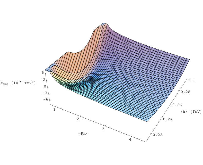
Figure 1: The total potential for the parameters given in (4). The minimum appears at the point $(\langle R_{0}\rangle,\langle h\rangle)=(1,\;0.258{\rm~{}TeV})$.

We can also compute effective masses² for the radion-$h_{0}$ system:

$$m^{2}_{h_{0}}=\frac{\partial^{2}V^{\rm 1-loop}_{\rm tot}}{\partial\langle h\rangle^{2}}\bigg{|}_{\rm min}=0.014{\rm~{}TeV}^{2}\,,$$

$$m^{2}_{r}=\frac{\partial^{2}V^{1-loop}_{\rm tot}}{\partial\langle r\rangle^{2}}\bigg{|}_{\rm min}=1.14\times 10^{-35}{\rm~{}TeV}^{2}\,,$$

$$m^{2}_{r\;h_{0}}=\frac{\partial^{2}V^{\rm 1-loop}_{\rm tot}}{\partial\langle r\rangle\partial\langle h\rangle}\bigg{|}_{\rm min}=3.38\times 10^{-20}{\rm~{}TeV}^{2}\,.$$ (36)

We have always chosen the parameter $\rho$ in such a way that the minimum of the complete potential appears at the point $\langle r\rangle\ll M_{\rm Pl}$, which implies $R_{0}\approx 1$ (see discussion below). In such a case the physical radius of the fifth dimension is given by the parameter $\rho$.

$m_{H}$ [TeV]	$m_{h}$ [TeV]	$m_{r}$ [$10^{-6}$ eV]	$\rho^{-1}$ [TeV]	$\langle h\rangle$ [TeV]	$\Lambda_{4}$ [$10^{-6}$ TeV]
0.10	0.098	3.5	0.49	0.265	$-7.90$
0.12	0.119	3.4	0.47	0.259	$-7.59$
0.14	0.139	3.3	0.47	0.255	$-7.36$
0.16	0.160	3.2	0.46	0.252	$-7.09$
0.18	0.181	3.0	0.44	0.250	$-6.68$
0.20	0.202	2.8	0.42	0.249	$-6.05$
0.22	0.225	2.4	0.39	0.247	$-5.06$

Table 1: Higgs boson and radion mass, the scale of the extra dimension $\rho^{-1}$, the Higgs-boson vacuum expectation values and the resulting cosmological constant, obtained for different input tree-level Higgs boson masses $m_{H}$.

Let us explain the way we adjust the $\rho$, which parametrizes the physical masses and couplings in 4d. The point is that we are interested in a specific range of the effective physical scales as seen in 4d, which we consider realistic. However, these physical scales depend on the expectation value of the radion, which we need to determine dynamically, and this dependence occurs through the factors that are powers of $e^{\alpha\langle r\rangle}$ (the parameters that are radion-independent are those that define the Lagrangian in 5d). To be able to follow the dynamical determination of the radion, we define auxiliary 4d parameters, which are radion-independent: $\lambda_{4},\,e_{4},\,g_{4}$ differ from the physical ones by the suitable powers of $e^{\alpha\langle r\rangle}$ and we note that the auxiliary parameters are equal to physical ones at $\langle R_{0}\rangle=e^{\alpha\langle r\rangle}\approx 1$. The usual approach would be to fix $\rho$, which sets the physical scale of the fifth dimension, to some convenient value, e.g. $\rho=1$, and to keep it constant during the calculations. However, the above reasoning suggests that the opposite is more convenient: in each model under discussion we shall fix the expectation value of the radion to be equal to unity, and achieve this by changing the value of $\rho$. It is obvious that physically this is a legal point of view. In 5d the meaningful quantity is in fact $2\pi\rho R_{0}$, and any change of $\langle R_{0}\rangle$ can be compensated by an adjustment of $\rho$, while keeping the parameters of the Lagrangian, hence the 5d model, unchanged. When we compactify and switch over to the 4d language the situation becomes slightly more complicated, since the 4d couplings, say $\lambda_{4}$, are related to the 5d ones by a power of $\rho$. Hence to stay in the same 5d model one would have to change $\lambda_{4}$ together with $\rho$. This is not what we want to do: we are interested in 4d models and keep 4d couplings constant. This is perfectly acceptable from the point of view of the 4d physics; one only needs to keep in mind that in the present picture different values of $\rho$ correspond to slightly different 5d couplings, hence slightly different 5d models. Having said this, let us define the procedure that brings us down to $\langle R_{0}\rangle=1$ and allows us to identify the physical masses in 4d in a straightforward manner. We start with an arbitrarily chosen value of $\rho$ and minimize the one-loop potential to find $\langle R_{0}\rangle$. Then we repeat the procedure, taking $\rho^{(1)}=\langle R_{0}\rangle\rho$. Then we repeat the steps again and again until we reach $\langle R_{0}\rangle\approx 1$, taking for each consecutive iteration $\rho^{(n)}=\langle R_{0}\rangle^{(n-1)}\rho^{(n-1)}$, where $n$ denotes the parameter of the $n$-th iteration. The procedure converges to $\langle R_{0}\rangle\approx 1$ within just a few iterations (as expected, since the physical size of the fifth dimension is $2\pi\rho\langle R_{0}\rangle$).

In addition, the calculations have been done for various values of the Higgs mass, and the results are listed in Table 1. We have chosen the tree-level Higgs boson mass to be in agreement with the electroweak measurements, i.e. roughly between $0.1$ TeV and $0.22$ TeV. It turns out that for $m_{H}\mathrel{\raise 1.29167pt\hbox{$>$\kern-7.5pt\lower 4.30554pt\hbox{$\sim$}}}0.26$ TeV the effective potential becomes unstable: the radion vacuum expectation value runs away to infinity. It is amusing to notice that $m_{H}=0.204$ TeV is the electroweak 95% CL upper bound on the SM Higgs boson mass [7]. The existence of the minimum is a result of an interplay between bosonic and fermionic contributions to the effective potential, so the largest Higgs mass for which we obtain stability is correlated with the top quark mass $m_{t}=0.175$ TeV. Therefore even though our toy model does not reflect all the features of the real 5d SM, it does nevertheless contain right mass scales. At the same time, it seems to favour the range of the Higgs boson mass that is also anticipated by the one-loop predictions of the SM. We find this nice agreement quite amusing. Note also in the table that the diagonal Higgs boson mass $m_{h}$ and the vacuum expectation values $\langle h\rangle$ are almost insensitive to the input, tree-level Higgs boson mass $m_{H}$; this is an obvious result of the very small mixing with the radion. The diagonal radion mass varies between $3.47\times 10^{-6}$ and $2.39\times 10^{-6}$ eV. The resulting size of the extra dimension, $\rho^{-1}\simeq 0.4$ – $0.5$ TeV, roughly agrees with the existing bound on the size of one universal extra dimension [8].

An important comment is in order here. From the 5d point of view the meaningful physical quantity is the physical size of the fifth dimension, which is given by $L_{\rm phys}=2\pi\rho\langle R_{0}\rangle$. Hence, at first sight, in various physical quantities the powers of $\rho$ should always multiply the same powers of $R_{0}$. However, this is not the case in the 4d Lagrangian and consequently, one finds in the effective potential an extra $R_{0}$ dependence that is not of the form $2\pi\rho R_{0}$. A closer inspection of the effective potential shows that this extra dependence on $\langle R_{0}\rangle$ has its roots in one additional power of $R_{0}$, which shows up in mass terms (both in those that originate from the $\mu^{2}$ scalar mass term and also in KK mass terms) in the 4d Lagrangian. However, this is correct and the reason can be seen in Eqs. (10) and (11). The point is that in (10) we have chosen to perform the Weyl rescaling using only the $R_{0}$, while $2\pi\rho$ becomes swallowed by the definition of the 4d Planck scale $M^{2}_{4}=2\pi\rho M^{3}_{5}$.

We have seen above that the radion field turns out to be very light and that it experiences a negligible mixing with the Higgs field: for $M_{h}=0.12$ TeV, we obtain $m_{r}=3.4\times 10^{-6}$ eV. Such a light field can modify the Newtonian gravity. A particle of mass $\sim 3.4\times 10^{-6}$ eV can mediate forces over a range of $\sim 37$ cm, see Ref. ([9]). Therefore such a small radion mass is excluded by experiments. It is possible to increase the radion mass by one or two orders of magnitude by rising the fermion masses (see also the next section), but heavy radion is not a natural phenomenon within the present set-up. As pointed out in [9] the explanation for a such low mass is due to the higher dimensional general covariance, which forbids a radion mass term in the higher dimensional theory. Therefore, in the flat 4d theory the radion mass term can appear only as a loop effect, and since the couplings of the radion are Planck-scale-suppressed, the resulting mass is naturally small.

5 The Higgsless theory

In the SM, the Higgs mechanism generates masses for the fermions and for the vector bosons. In the Higgsless theory one may assume that the fermion masses emerge from some additional dynamical mechanism [10]– [13], e.g. by the fermion condensation, while the masses of the vector bosons are due to a global breakdown of the gauge symmetry by boundary conditions imposed along extra dimensions. This is a noteworthy alternative to the usual Higgs mechanism, but also a particularly clear limit of the general case considered in the earlier sections, thus of particular interest to us.

Let us begin the discussion with the model that does not contain a 5d scalar field

$$S=S_{g}+S_{f}+S_{v}+S_{gf}\,,$$ (37)

where $S_{g}$ denotes the Einstein–Hilbert action (2) and the action for fermions and vector boson is given by

$$S_{f}=\int_{0}^{L}dy\int d^{4}x\sqrt{G}\left[{\rm i}\overline{\psi}\gamma^{M}(\partial_{M}-{\rm i}e_{5}A_{M})\psi+{\rm i}\overline{\lambda}\gamma^{M}\partial_{M}\lambda-\left(m_{5}\overline{\psi}\lambda+\hbox{H.c.}\right)\right]$$ (38)

and

$$S_{v}+S_{gf}=\int_{0}^{L}dy\int d^{4}x\sqrt{G}\left\{-\frac{1}{4}F^{MN}F_{MN}-\frac{1}{2\xi}\left[\partial_{\mu}A^{\mu}-\xi\partial_{5}A_{5}\right]^{2}\right\}\,,$$ (39)

respectively. The Yukawa interaction present in the Lagrangian (7) has been replaced here by the 5d mass term $m_{5}\overline{\psi}\lambda$. Here again we require the invariance of the action with respect to the transformations (5) and (6), which eliminates the possibility of diagonal fermionic mass terms. Here, however, we must modify the set-up employed in Section 2 and assign the U(1) charge to the fermion $\lambda$ in such a way that the mixed mass term $\overline{\psi}\lambda$ is gauge-invariant, i.e. $Q_{U(1)}(\lambda)=Q_{U(1)}(\psi)$ and $\gamma^{M}\partial_{M}\lambda\rightarrow\gamma^{M}(\partial_{M}-{\rm i}e_{5}A_{M})\lambda$. Note, however, that in the one-loop calculation of the effective potential for $r$, which we will perform here, these two cases, that is invariant and non-invariant 5d fermion mass terms, are indistinguishable and lead to identical conclusions about the stability of the scalar sector.

To obtain masses for the vector bosons we construct an orbifold $S^{1}/(Z_{2}\times Z_{2}^{{}^{\prime}})$ such that the action of the parities on the circle $S^{1}$ is the following: $Z_{2}$: $y\to-y$ and $Z_{2}^{{}^{\prime}}$: $L/2+y\to L/2-y$. Their action on the field space reads:

$$Z_{2}:\;\;\;\;\;\; A_{\mu}(x,y)=A_{\mu}(x,-y),\;\;\;A_{5}(x,y)=-A_{5}(x,-y)$$ (40)

$$Z_{2}^{{}^{\prime}}:\;\;\;\;\;\; A_{\mu}(x,L/2+y)=-A_{\mu}(x,L/2-y),\;\;\;A_{5}(x,L/2+y)=A_{5}(x,L/2-y)\,.$$ (41)

So, we have assumed $(+,-)$ and $(-,+)$ parities for $A_{\mu}$ and $A_{5}$, respectively. The fermionic boundary conditions remain the same as in the Higgs-like model, i.e. the right- and left-handed modes transform as $(+,+)$ and $(-,-)$, respectively. Therefore the fermions are periodic with a period $L$. The addition of the second requirement (41) is a crucial modification of the set-up defined in Section 2. This condition causes the breakdown of the gauge symmetry, since (40) alone leads to 4d theory, which is U(1) invariant. A consequence of (41) is that the gauge fields can no longer be periodic; in fact, one finds that the conditions (40) and (41) can be consistent only if the gauge fields are antiperiodic: 

$$A_{\mu}(x,y+L)=-A_{\mu}(x,y)\;\;\;A_{5}(x,y+L)=-A_{5}(x,y)\,.$$ (42)

This is acceptable as long as the Lagrangian remains invariant under the twist operator: $T:\;\;A_{M}\to-A_{M}$. Even more, for consistency, the Lagrangian must be invariant under both $Z_{2}$ parities acting with respect to each brane. The symmetry under $Z_{2}$ is evident. For $Z_{2}^{{}^{\prime}}$, however, one finds that the interaction between the vector boson and fermions through the covariant derivative does not fulfil this requirement, as it is antisymmetric

$$\left[\bar{\psi}\gamma^{M}e_{5}A_{M}\psi\right](L/2+y)=-\left[\bar{\psi}\gamma^{M}e_{5}A_{M}\psi\right](L/2-y)\,.$$ (43)

In order to make the set-up consistent, let us assume that the gauge coupling is odd under $Z_{2}^{{}^{\prime}}$, so we replace $e_{5}$ by $\epsilon(y)e_{5}$ with

$$\epsilon(y)=\left\{\begin{array}[]{ccc}&\vdots&\\ -1&{\rm for}&-3L/2<y<-L/2\\ +1&{\rm for}&-L/2<y<L/2\\ -1&{\rm for}&+L/2<y<3L/2\\ &\vdots&\end{array}\right.$$ (49)

Then the Lagrangian is invariant under both $Z_{2}$ parities. Let us note that in the above construction we have not introduced localized brane terms into the action. As a consequence, each field which is odd with respect to the given brane must vanish on that brane. The gauge transformations are not allowed to generate such singular terms, hence one must require that the gauge variations of the vector bosons do vanish at the ‘odd’ fixed point. To be more specific let us consider a gauge transformation with a parameter $\Lambda(x,y)$:

$$\psi\longrightarrow e^{-{\rm i}\epsilon e_{5}\Lambda}\psi\,,\quad\lambda\longrightarrow e^{-{\rm i}\epsilon e_{5}\Lambda}\lambda\,,\quad A_{M}\longrightarrow A_{M}+\partial_{M}\Lambda\,.$$ (50)

The requirement that such a gauge transformation does not change parities of the fields implies that $\Lambda$ is $Z_{2}$-even with respect to $y=0$ and $Z_{2}^{{}^{\prime}}$-odd with respect to $y=L/2$. It is interesting to see that the above conditions remove the global $U(1)$ transformations from the theory. This is consistent with the fact that boundary conditions break globally the group of gauge transformations: not even the global subgroup is left in the effective 4d model. Models with jumping gauge couplings were considered before in the literature, see [14]–[16]. Note that after introducing the jumping coupling the observer who travels around the circle will see precisely the same coupling between the fermions and the gauge field after passing the brane at $y=L/2$ as before. Hence the physics on both half-circles remains the same.

Decomposition of the 5d metric tensor and the KK expansion of the fermionic fields is the same as in the previous sections. The KK expansion of the vector boson fields reads

$$A^{\mu}(x,y) = \frac{1}{\sqrt{\pi\rho}}\sum_{n=0}^{\infty}A_{n}^{\mu}(x)\cos\left[y\left(m_{n}+\frac{\pi}{L}\right)\right]\,,$$

$$A^{5}(x,y) = \frac{1}{\sqrt{\pi\rho}}\sum_{n=0}^{\infty}A_{n}^{5}(x)\sin\left[y\left(m_{n}+\frac{\pi}{L}\right)\right]\,.$$ (51)

where $m_{n}=2\pi n/L$. The following mass terms of the vector bosons are obtained:

$$m^{2}_{A_{\mu n}}=e^{-3\alpha\langle r\rangle}\left(\frac{\pi}{L}+m_{n}\right)^{2},\;\;\;\;\;\;m^{2}_{A_{5n}}=0\,.$$ (52)

The scalar modes $A_{5n}$ are the Goldstons bosons that become longitudinal components of massive $A_{\mu n}$.

The DPQ procedure leads to

$$V^{(\infty)}_{A_{\mu}} = 0\,,$$

$$V^{(R)}_{A_{\mu}} = -e^{-6\alpha\langle r\rangle}\frac{3}{64\pi^{6}\rho^{4}}{\rm Li_{5}}(-1)\,.$$ (53)

The total contribution of the vector fields to the one-loop effective potential reads

$$V^{\rm 1-loop}_{v}=\frac{3}{2}\left(V^{(\infty)}_{A_{\mu}}+V^{(R)}_{A_{\mu}}\right)\,.$$ (54)

The mass terms of the fermions are

$$m_{\psi_{n}} = -e^{-\frac{3}{2}\alpha\langle r\rangle}m_{n}\,,$$

$$m_{\lambda_{n}} = e^{-\frac{3}{2}\alpha\langle r\rangle}m_{n}\,,$$

$$m_{\psi_{n}\;\lambda_{n}} = -e^{-\frac{1}{2}\alpha\langle r\rangle}m_{4}\,,$$

$$m_{\psi_{0R}\;\lambda_{0L}} = -e^{-\frac{1}{2}\alpha\langle r\rangle}m_{4}\,,$$ (55)

where $m_{4}=m_{5}/\sqrt{2\pi\rho}$.

The fermionic contribution to the one-loop effective potential reads:

$$V^{\rm 1-loop}_{f}=-4\left(V^{(\infty)}_{f}+V^{(R)}_{f}\right)\,,$$ (56)

where

$$V^{(\infty)}_{f} = e^{\frac{3}{2}\alpha\langle r\rangle}\frac{\rho}{60\pi}|m_{f}|^{5}\,,$$

$$V^{(R)}_{f} = -e^{-6\alpha\langle r\rangle}\frac{1}{64\pi^{6}\rho^{4}}\left[x_{f}^{2}{\rm Li_{3}}\left(e^{-x_{f}}\right)+3x_{f}{\rm Li_{4}}\left(e^{-x_{f}}\right)+3{\rm Li_{5}}\left(e^{-x_{f}}\right)\right]\,.$$ (57)

We have defined $m_{f}=e^{-\frac{1}{2}\alpha\langle r\rangle}m_{4}$ and $x_{f}=e^{\frac{3}{2}\alpha\langle r\rangle}2\pi\rho|m_{f}|$. The total one-loop potential including all contributions reads

$$V^{\rm 1-loop}_{\rm tot}=V^{\rm 1-loop}_{v}+V^{\rm 1-loop}_{f}\,.$$ (58)

We have again analysed the effective potential as a function of $\langle r\rangle$. Numerical calculations have been done for the following choice of parameters:

$$\kappa=0.1{\rm~{}TeV}\,,\quad M_{4}=2\times 10^{15}{\rm~{}TeV}$$ (59)

and for various values of the fermion mass. We have chosen the parameter $\rho$ in such a way that the minimum of the complete potential appears at the point $\langle r\rangle\ll M_{\rm Pl}$, which implies $R_{0}\approx 1$ (see Fig. 2). In such a case the physical radius of the fifth dimension is given by the parameter $\rho$. We have found the mass of the radion in the form

$$m^{2}_{r}=\frac{\partial^{2}V^{\rm 1-loop}_{\rm tot}}{\partial\langle r\rangle^{2}}\bigg{|}_{\rm min},$$ (60)

Figure 2: The total potential for the parameters given in (59) and for $m_{4}=0.175{\rm~{}TeV}$. The minimum appears at the point $\langle R_{0}\rangle=1$.

and the value of the scalar potential at the minimum $\Lambda_{4}$, which is the cosmological constant. We have displayed the results in Table 2. One can easily find the following approximate relations between the mass of the fermion and the other physical parameters

$$\rho^{-1}=c_{\rho}m_{4},\quad m_{r}=c_{m}\frac{m_{4}^{2}}{M_{\rm Pl}},\quad\Lambda_{4}=-c_{\Lambda}m_{4}^{4}\,,$$ (61)

where

$$c_{\rho}=1.9,\quad c_{m}=5.2\times 10^{-2},\quad c_{\Lambda}=9.6\times 10^{-3}\,.$$ (62)

$m_{4}$ [TeV]	$\rho^{-1}$ [TeV]	$m_{r}$ [eV]	$\Lambda_{4}$ [TeV4]
0.080	0.15	$6.7\times 10^{-7}$	$-3.93\times 10^{-7}$
0.175	0.33	$3.2\times 10^{-6}$	$-8.99\times 10^{-6}$
0.350	0.66	$1.3\times 10^{-5}$	$-1.44\times 10^{-4}$
0.700	1.32	$5.1\times 10^{-5}$	$-2.30\times 10^{-3}$
1.400	2.65	$2.1\times 10^{-4}$	$-3.69\times 10^{-2}$
2.800	5.30	$8.2\times 10^{-4}$	$-5.90\times 10^{-1}$

Table 2: Radion masses together with the scale of the extra dimension $\rho^{-1}$ and the resulting cosmological constant, obtained for different input fermion masses $m_{4}$.

It is seen from the table and relations (62) that the dependence of the radion mass on the input bulk fermion mass, $m_{5}=\sqrt{2\pi\rho}m_{4}$, is quite strong. The result is the variation of the radion mass between $6.7\times 10^{-7}$ and $8.2\times 10^{-4}$ eV. Notice that the value of the cosmological constant that we have obtained is much larger than cosmological constraints. However, one can cancel it by the renormalization counterterms. To obtain a constant counterterm in the 4d theory, after the Weyl rescaling, the following corrections can be added to the 5d action:

$$\delta S=\int d^{5}x\sqrt{G}\sqrt{-G_{55}}\delta\Lambda+\int d^{4}x\sqrt{-g}G_{55}\delta\lambda_{0}\Big{|}_{y=0}+\int d^{4}x\sqrt{-g}G_{55}\delta\lambda_{\pi}\Big{|}_{y=\pi\rho}\,,$$ (63)

where the first term spoils 5d covariance in the bulk, but is acceptable from the 4d point of view (also, it is considered here as a one-loop-order counterterm). These counterterms can be used to make the 4d one-loop cosmological constant vanish without violating the 4d Lorentz invariance and, more importantly, without destabilizing the scalar potential for the radion.

It can be seen that the presence of the 5d bulk mass term for the fermions is crucial for the stabilization. The minimum at a finite value of the radion disappears when $m_{5}$ approaches zero (this is the decompactification limit, and the radion expectation value runs away toward infinity). The point is that the dependence of the tree-level fermionic mass term on the radion is different from that of the KK mass terms, and the presence of the minimum is the result of the interplay between the terms denoted as $V_{f}^{(\infty)}$ and $V_{f}^{(R)}$ in (5), the first of which depends on the tree-level fermionic mass, the second on the KK masses.

6 Summary

We have discussed the stabilization of the scalar sector including the radion, in the QED-like gauge model with one universal extra dimension; with gauge symmetry broken by the 5d Higgs mechanism and in the case where the breaking occurs because of the boundary conditions imposed on the gauge fields. The stabilization is due to the fermionic contribution to the effective potential. In fact, for the stabilization to take place, the bosonic contribution must be balanced by the fermionic one, hence the scales of these two cannot differ too much. However, one does not need (softly broken) supersymmetry to achieve the stabilization: it can be arranged in models born in universal extra dimensions for a reasonably wide range of couplings and mass scales. One does not need complicated models or unreasonable fine-tunings; even the simple QED-like set-up is sufficient. We expect the generic features of our mechanism to hold also in the case of (broken) supersymmetry, even in the presence of a larger number of moduli fields (see also [17]).

It can be seen that the presence of the 5d bulk mass term for the fermions is crucial for the stabilization. For instance, in the Higgs model discussed in Section 4, the minimum at finite values of the fields in the radion–scalar hyperplane disappears when $g_{5}$ (so consequently the mass of the zero-mode fermion vanishes) approaches zero (this is the decompactification limit, and the radion vacuum expectation value runs away toward infinity). The point is that the dependence of the tree-level fermionic mass term on the radion is different from that of the KK mass terms, and the presence of the minimum is the result of the interplay between the terms denoted as $V_{f}^{(\infty)}$ and $V_{f}^{(R)}$ in (4), the first of which depends on the tree-level fermionic mass, the second on the KK masses. The situation is very similar in the Higgsless case, for which the relevant formula is (5).

One may also consider localized brane mass terms for the fermions of the form $G_{55}\delta(x^{5}-x^{5}_{b})m_{b}\overline{\psi}\lambda$. However, these terms play the role of sources in the equations of motion, and they are cancelled by discontinuities in the bulk fermionic configurations. Their role is to impose boundary conditions on the fields, hence they affect the quantization of the masses of the KK modes. This effect on its own does not create a minimum: the bulk terms described above are still needed.

It is interesting to watch correlation between the various physical parameters that arise upon the stabilization of the scalar sector. For a Higgs mass larger than $0.26$ TeV, we observe that there appears an instability in the effective potential in the direction of the radion - its vacuum expectation value runs away to infinity (decompactification limit). It is interesting to note that $m_{H}\simeq 0.204$ TeV is the electroweak 95% CL upper bound on the Higgs boson mass. Therefore even though our toy model does not reflect all the features of the real 5d SM, it nevertheless favours the range of Higgs boson masses that is also anticipated by the one-loop predictions of the Standard Model. It turns out that, for parameter values adopted here for the Higgs case, the radion run-away is the primary instability in the model, not the large-$h$ instability discussed in [1].

It is also interesting to note that the cosmological constant may be cancelled by suitable counterterms, in such a way that stabilization of scalars is not affected.

Acknowledgements

B.G. is supported in part by the State Committee for Scientific Research (Poland) under grant 1 P03B 078 26 in the period 2004–2006. Z.L. thanks the Theory Division at CERN for hospitality. This work was partially supported by the EC Contract HPRN-CT-2000-00152 for the years 2000–2004, by the Polish State Committee for Scientific Research grants KBN 2P03B 001 25 (Z.L.) and by KBN 2P03B 124 25 (R.M.), and by POLONIUM 2004.

Appendix

Here we provide some details of the dimensional reduction (in the Higgs case) and calculation of the effective potential generated by a tower of KK modes.

The KK expansion of the fields living on $S^{1}/Z_{2}$ gives

$$A^{\mu}(x,y) = \frac{1}{\sqrt{2\pi\rho}}\left[A_{0}^{\mu}(x)+\sqrt{2}\sum_{n=1}^{\infty}A_{n}^{\mu}(x)\cos(m_{n}y)\right]\,,$$

$$A^{5}(x,y) = \frac{1}{\sqrt{\pi\rho}}\sum_{n=1}^{\infty}A_{n}^{5}(x)\sin(m_{n}y)\,,$$

$$\phi(x,y) = \frac{1}{\sqrt{2\pi\rho}}\left[\phi_{0}(x)+\sqrt{2}\sum_{n=1}^{\infty}\phi_{n}(x)\cos(m_{n}y)\right]\,,$$

$$\psi(x,y) = \frac{1}{\sqrt{2\pi\rho}}\left[\psi_{R0}(x)+\sqrt{2}\sum_{n=1}^{\infty}\left[\psi_{Rn}(x)\cos(m_{n}y)+\psi_{Ln}(x)\sin(m_{n}y)\right]\right]\,,$$

$$\lambda(x,y) = \frac{1}{\sqrt{2\pi\rho}}\left[\lambda_{L0}(x)+\sqrt{2}\sum_{n=1}^{\infty}\left[\lambda_{Ln}(x)\cos(m_{n}y)+\lambda_{Rn}(x)\sin(m_{n}y)\right]\right]\,,$$ (A.1)

where $m_{n}=2\pi n/L$.

Expanding the 4d Lagrangian around $h_{0}\rightarrow h_{0}+\langle h\rangle$, $r\rightarrow r+\langle r\rangle$, the following scalar mass terms are obtained in the Landau gauge:

$$m^{2}_{h_{0}} = e^{-\alpha\langle r\rangle}\left(-\mu^{2}+3\lambda_{4}\langle h\rangle^{2}\right)\,,$$

$$m^{2}_{\chi_{0}} = e^{-\alpha\langle r\rangle}\left(-\mu^{2}+\lambda_{4}\langle h\rangle^{2}\right)\,,$$

$$m^{2}_{h_{n}} = e^{-\alpha\langle r\rangle}\left(-\mu^{2}+3\lambda_{4}\langle h\rangle^{2}+e^{-2\alpha\langle r\rangle}m_{n}^{2}\right)\,,$$

$$m^{2}_{\chi_{n}} = e^{-\alpha\langle r\rangle}\left(-\mu^{2}+\lambda_{4}\langle h\rangle^{2}+e^{-2\alpha\langle r\rangle}m_{n}^{2}\right)\,,$$

$$m^{2}_{r} = \alpha^{2}e^{-\alpha\langle r\rangle}\left(-\frac{1}{2}\mu^{2}\langle h\rangle^{2}+\frac{1}{4}\lambda_{4}\langle h\rangle^{4}+\frac{\mu^{4}}{4\lambda_{4}}\right)\,,$$

$$m^{2}_{r\;h_{0}} = -\alpha e^{-\alpha\langle r\rangle}\left(-\mu^{2}\langle h\rangle+\lambda_{4}\langle h\rangle^{3}\right)\,,$$

$$m^{2}_{A_{5n}} = e^{-\alpha\langle r\rangle}e_{4}^{2}\langle h\rangle^{2}\,,$$

$$m^{2}_{A_{5n}\;\chi_{n}} = -e^{-2\alpha\langle r\rangle}e_{4}\langle h\rangle m_{n}\,,$$ (A.2)

where $\alpha$, $\lambda_{4}$, $e_{4}$ are defined in the main text.

For vector bosons the following mass terms are obtained

$$~{}m^{2}_{A_{\mu n}} = e^{-\alpha\langle r\rangle}\left(e_{4}^{2}\langle h\rangle^{2}+e^{-2\alpha\langle r\rangle}m_{n}^{2}\right)\,,$$

$$m^{2}_{A_{\mu 0}} = e^{-\alpha\langle r\rangle}e_{4}^{2}\langle h\rangle^{2}\,.$$ (A.3)

The masses of the fermions are given by

$$m_{\psi_{n}} = -e^{-\frac{3}{2}\alpha\langle r\rangle}m_{n}\,,$$

$$m_{\lambda_{n}} = e^{-\frac{3}{2}\alpha\langle r\rangle}m_{n}\,,$$

$$m_{\psi_{n}\;\lambda_{n}} = -e^{-\frac{1}{2}\alpha\langle r\rangle}\frac{g_{4}}{\sqrt{2}}\langle h\rangle\,,$$

$$m_{\psi_{0R}\;\lambda_{0L}} = -e^{-\frac{1}{2}\alpha\langle r\rangle}\frac{g_{4}}{\sqrt{2}}\langle h\rangle\,,$$ (A.4)

where $g_{4}=g_{5}/\sqrt{2\pi\rho}$.

For the purpose of this paper we have adopted the regularization scheme worked out by Delgado et al. (DPQ, see [3]) to compute the contribution of the KK tower to the effective potential. Let us briefly recall the basic result obtain by DPQ.
Starting from the generic formula

$$V(\phi)=\frac{1}{2}\int\frac{d^{4}p}{(2\pi)^{4}}\sum_{0}^{\infty}\log{[l^{2}E^{2}+n^{2}\pi^{2}]}\,,$$ (A.5)

where $E^{2}\equiv p^{2}+m^{2}(\phi)$, $m^{2}(\phi)$ are the background-field-dependent mass squared of the KK modes and $l=\pi\rho$. With the help of the $\overline{MS}$ renormalization scheme one obtains

$$V=\frac{1}{2}(V^{(\infty)}+V^{(R)}+V^{0})$$ (A.6)

where

$$V^{(\infty)} = \frac{\rho}{60\pi}m^{5}(\phi)\,,$$

$$V^{0} = \frac{1}{64\pi^{2}}m^{4}(\phi)\left[\log\left(\frac{m^{2}(\phi)}{k^{2}}\right)-\frac{3}{2}\right]\,,$$

$$V^{(R)} = -\frac{1}{64\pi^{6}\rho^{4}}(x^{2}{\rm Li}_{3}(e^{-x})+3x{\rm Li}_{4}(e^{-x})+3{\rm Li}_{5}(e^{-x}))\,.$$ (A.7)

In the above the $x$ is given by $x=2\pi\rho\sqrt{m^{2}(\phi)}$, $\kappa$ is the renormalization scale, and ${\rm Li}_{n}(x)=\sum_{s=1}^{\infty}\frac{x^{s}}{s^{n}}$ is the polylogarithm function.

References

• [1] P. Bucci and B. Grzadkowski, “The effective potential and vacuum stability within universal extra dimensions,” Phys. Rev. D 68, (2003) 124002 [arXiv:hep-ph/0304121].
• [2] B. Grzadkowski and M. Toharia, “Low-energy effective theory from a non-trivial scalar background in extra dimensions,” arXiv:hep-ph/0401108.
• [3] A. Delgado, A. Pomarol and M. Quiros, “Supersymmetry and electroweak breaking from extra dimensions at the TeV scale,” Phys. Rev. D 60, (1999) 095008 [arXiv:hep-ph/9812489].
• [4] I. Antoniadis, “A Possible New Dimension At A Few Tev,” Phys. Lett. B 246 (1990) 377.
• [5] I. Antoniadis, S. Dimopoulos, A. Pomarol and M. Quiros, “Soft masses in theories with supersymmetry breaking by TeV-compactification,” Nucl. Phys. B 544 (1999) 503 [arXiv:hep-ph/9810410].
• [6] E. Ponton and E. Poppitz, “Casimir energy and radius stabilization in five and six dimensional orbifolds,” JHEP 0106, (2001) 019 [arXiv:hep-ph/0105021].
• [7] K. Hagiwara et al. [Particle Data Group Collaboration], “Review of Particle Physics,” Phys. Rev. D 66, (2002) 010001 .
• [8] T. Appelquist, H. C. Cheng and B. A. Dobrescu, “Bounds on universal extra dimensions,” Phys. Rev. D 64, (2001) 035002 [arXiv:hep-ph/0012100]; K. Agashe, N. G. Deshpande and G. H. Wu, “Universal extra dimensions and b $\to$ s gamma,” Phys. Lett. B 514, (2001) 309 [arXiv:hep-ph/0105084]; A. J. Buras, M. Spranger and A. Weiler, “The impact of universal extra dimensions on the unitarity triangle and rare K and B decays,” arXiv:hep-ph/0212143; K. Agashe, N. G. Deshpande and G. H. Wu, “Can extra dimensions accessible to the SM explain the recent measurement of anomalous magnetic moment of the muon?,” Phys. Lett. B 511, (2001) 85 [arXiv:hep-ph/0103235]; T. Appelquist and B. A. Dobrescu, “Universal extra dimensions and the muon magnetic moment,” Phys. Lett. B 516, (2001) 85 [arXiv:hep-ph/0106140].
• [9] Z. Chacko and E. Perazzi, “Extra dimensions at the weak scale and deviations from Newtonian gravity,” arXiv:hep-ph/0210254.
• [10] C. Csaki, C. Grojean, H. Murayama, L. Pilo and J. Terning, “Gauge theories on an interval: Unitarity without a Higgs,” arXiv:hep-ph/0305237.
• [11] R. Barbieri, A. Pomarol and R. Rattazzi, “Weakly coupled Higgsless theories and precision electroweak tests,” arXiv:hep-ph/0310285.
• [12] C. Csaki, C. Grojean, J. Hubisz, Y. Shirman and J. Terning, “Fermions on an interval: Quark and lepton masses without a Higgs,” arXiv:hep-ph/0310355.
• [13] R. Barbieri, “Electroweak symmetry breaking as of 2003, on the way to the Large Hadron Collider,” arXiv:hep-ph/0312253.
• [14] A. Falkowski, Z. Lalak and S. Pokorski, “Supersymmetrizing branes with bulk in five-dimensional supergravity,” Phys. Lett. B 491, (2000) 172 [arXiv:hep-th/0004093].
• [15] E. Bergshoeff, R. Kallosh and A. Van Proeyen, “Supersymmetry in singular spaces,” JHEP 0010, (2000) 033 [arXiv:hep-th/0007044].
• [16] Z. Lalak and R. Matyszkiewicz, “Singular gauge transformations and supersymmetry breakdown on warped orbifolds,” Phys. Lett. B 583 (2004) 364 [arXiv:hep-th/0310269].
• [17] G. von Gersdorff, M. Quiros and A. Riotto, “Scherk-Schwarz supersymmetry breaking with radion stabilization,” arXiv:hep-th/0310190.