SLAC-PUB-10365
LES HOUCHES “PHYSICS AT TEV COLLIDERS 2003” BEYOND THE STANDARD MODEL WORKING GROUP: SUMMARY REPORT

Abstract

The work contained herein constitutes a report of the “Beyond the Standard Model” working group for the Workshop “Physics at TeV Colliders”, Les Houches, France, 26 May–6 June, 2003. The research presented is original, and was performed specifically for the workshop. Tools for calculations in the minimal supersymmetric standard model are presented, including a comparison of the dark matter relic density predicted by public codes. Reconstruction of supersymmetric particle masses at the LHC and a future linear collider facility is examined. Less orthodox supersymmetric signals such as non-pointing photons and R-parity violating signals are studied. Features of extra dimensional models are examined next, including measurement strategies for radions and Higgs’, as well as the virtual effects of Kaluza Klein modes of gluons. An LHC search strategy for a heavy top found in many little Higgs model is presented and finally, there is an update on LHC $Z^{\prime}$ studies.

Abstract

An accord specifying a unique set of conventions for supersymmetric extensions of the Standard Model together with generic file structures for (1) supersymmetric model specifications and input parameters, (2) electroweak scale supersymmetric mass and coupling spectra, and (3) decay tables is defined, to provide a universal interface between spectrum calculation programs, decay packages, and high energy physics event generators.

Abstract

We present and describe an internet resource which allows the user to compare different calculations of MSSM spectra. After providing (currently mSUGRA) SUSY breaking input parameters, the spectra predicted by the publicly available programs ISASUGRA, SOFTSUSY, SPHENO and SUSPECT are output by the resource. The variance and range of results is also produced.

Abstract

We compare the relic density of neutralino dark matter within the minimal supergravity model (mSUGRA) using four different public codes for supersymetric spectra evaluation.

Abstract

SFITTER is a new tool to determine supersymmetric model parameters from collider measurements. It allows to perform a grid search for the minimal $\chi^{2}$ and/or a fit of a given model. Currently, the model parameters in the general MSSM or in a gravity mediated SUSY breaking model can be tested using a given set of mass, branching ratio and cross section measurements.

Abstract

We present the Fortran code SDECAY, a program which calculates the decay widths and branching ratios of all supersymmetric particles in the Minimal Supersymmetric Standard Model, including higher order effects. The usual two-body decays of sfermions and gauginos as well as the three-body decay modes of charginos, neutralinos and gluinos are included. Furthermore, the three-body and even the four-body decays of top squarks are calculated. The important loop-induced decays, the QCD corrections to the two-body widths involving strongly interacting particles and the dominant electroweak effects to all processes are evaluated as well.

Abstract

Results are presented of a feasibility study of techniques for measuring the mass of the lightest chargino at the CERN LHC. These results suggest that for one particular mSUGRA model a statistically significant chargino signal can be identified and the chargino mass reconstructed with a precision $\sim$ 11% for $\sim$ 100 fb^-1 of data.

Abstract

We demonstrate how the interplay of a future $e^{+}e^{-}$ LC at its first stage with $\sqrt{s}\;\raisebox{-3.87495pt}{$\textstyle\stackrel{{\scriptstyle\textstyle<}}{{\sim}}$}\;500$ GeV and of the LHC could lead to a precise determination of the fundamental SUSY parameters in the gaugino/higgsino sector without assuming a specific supersymmetry breaking scheme. The results are shown for the benchmark scenario SPS1a, taking into account realistic errors for the masses and cross sections measured at the LC with polarised beams and mass measurements at the LHC.

Abstract

When several sparticle masses are known, the kinematics of SUSY decay processes observed at the LHC can be solved if the cascade decays contain sufficient steps. We demonstrate four examples of this full reconstruction technique applied to channels involving leptons, namely a) gluino mass determination, b) sbottom mass determination, c) LSP momentum reconstruction, and d) heavy higgs mass determination.

Abstract

There has recently been interest in “a new reconstruction technique for SUSY processes at the LHC”. The primary intention of this note is to describe a modification to the way the technique is used. This modification suggests the method is much more powerful than originally proposed. We demonstrate that, in principle at least, the method does not need to rely on input from other experiments. We show that the method is capable of standing on its own, and is able to measure the masses of all the sparticles participating in the relevant decay chains. Results from other experiments such as a future linear collider may easily be incorporated if desired.

Abstract

Measurement of non-pointing photons is a key issue to study the gauge mediation models at the CERN LHC. In this article we study the $\theta$ resolution of non-pointing photons with the ATLAS electromagnetic calorimeter, and discuss the impacts to the study of the gauge mediation models.

Abstract

We study an MSSM model with bilinear R-parity violation which is capable of explaining neutrino data while leading to testable predictions for ratios of LSP decay rates. Further, we estimate the precision with which such measurements could be carried out at the LHC.

Abstract

We examine resonant slepton production at the LHC with gravitinos in the final state. We investigate two cases: (i) where the slepton undergoes gauge decay into neutralino and a lepton, followed by the neutralino decay into a photon and a gravitino, and (ii) direct decays of a slepton into a lepton and a gravitino. We show how to accurately reconstruct both the slepton and neutralino masses in the first case, and the slepton mass in the second case for 300 fb^-1 of integrated luminosity at the LHC.

Abstract

We begin an examination of the effects of mixing between the radion of the Randall-Sundrum (RS) model and the Higgs fields of the Two-Higgs-Doublet model as would be motivated by, $e.g.$, supersymmetry. Preliminary results for the shifts in various particle masses and couplings are obtained.

Abstract

Assuming flat universal extra dimensions, we demonstrate that for a light Higgs boson the process $pp\to W^{*}W^{*}+X\to{\rm Higgs,graviscalars}+X\to{\rm invisible}+X$ will be observable at the $5\leavevmode\nobreak\ \sigma$ level at the LHC over the portion of the Higgs-graviscalar mixing ($\xi$) and effective Planck mass ($M_{D}$) parameter space where channels relying on visible Higgs decays fail to achieve a $5\leavevmode\nobreak\ \sigma$ signal. Further, we show that for some values of $\delta$ and $\xi\sim O(1)$ the invisible decay signal can probe values of $M_{D}$ up to and possibly above those probed by the ($\xi$-independent) jets/$\gamma$ + missing energy signal from graviton radiation. We also discuss various effects, such as Higgs decay to two graviscalars, that could become important when $m_{h}/M_{D}$ is of order 1.

Abstract

In the context of a TeV^-1 size extra dimensional model, we consider the lightest Higgs boson as an admixture of brane and bulk scalar fields. We find that at the Tevatron Run 2 or at the LC the Higgs signal is suppressed. Meanwhile, at the LHC or at CLIC one might find highly enhanced production rates. This will enable the latter experiments to distinguish between the extra dimensional and the SM for $M_{c}$ up to about 6 TeV and perhaps determine the extra-dimensional location of the lightest Higgs boson.

Abstract

In this work, we present results for dijet distributions at the LHC with the assumption of a TeV size extra dimension. In our calculation, we included the virtual effects of gluonic Kaluza-Klein state exchanges, as well as the modified running of the strong coupling constant (but restricted our numerical study to the case of standard $\alpha_{S}$ evolution). Computing the transverse momentum distribution of dijets, we found that the LHC is able to discover a single extra dimension up to $M_{c}\sim 15$ TeV.

Abstract

A recent idea of solving the ’little hierarchy’ between physical mass of the Higgs boson and present limit of relatively low cut off scale of about 10 TeV has a vector-like new heavy quark Top as one of the additional particles. The potential of CMS experiment at LHC to discover it has been studied using the available phenomenology for collider experiments.

Part I Introduction

B.C. Allanach

The workshop took place at the école de physique in the lee of Mont Blanc, and lasted for two weeks. Computer systems were installed by the helpful LAPP staff for use by participants throughout the workshop. The first two days consisted of plenary talks intended to stimulate ideas and the proposition of projects. A couple of further plenary seminars on hot topics occured sporadically later in the workshop. The Beyond the Standard Model working group (convened by M Battaglia, M Nojiri, T Rizzo, A de Roeck, D Tovey, M Spiropoulu and the author) held a meeting on the second evening to set individual projects for small groups of interested parties. This report contains a summary of the fruits of participants’ labour during and after the workshop on those projects. The projects were phenomenological studies of both supersymmetric and non-supersymmetruc models and. The report first discusses the studies of supersymmetric models and then those of extra dimensions. We close with an update on $Z^{\prime}$ studies.

At the time of the workshop the Tevatron and DESY collider runs were proceeding, and the start-up of the Large Hadron Collider (LHC) was eagerly awaited. Many hopes are concentrating upon the production and detection of supersymmetric (SUSY) particles at these colliders. Although an immense amount of literature has been accumulated on SUSY phenomenology, there is still a large amount of work to do because of its complexity and the abundance of models of SUSY breaking. The models predict different cascade chains leading to radically differing signals in experiments. In order to facilitate the phenomenological study of SUSY models, we need to both calculate the sparticle spectrum and also we need to simulate events. These two calculations are typically performed by seperate calculational tools. For each calculation, there exist several competing tools performing the same task with different approximations or assumptions. A common interface between the different tools has clear advantages, and much time was spent at (and after) the workshop arguing, debating and negotiating the various conventions. The write-up of this “SUSY Les Houches Accord” constitutes part II of this report. A form-based web tool is presented in part III in which one can determine the spectra from mSUGRA models via the different public sparticle spectrum generators. The difference between the predictions of the different generators gives an idea of the theoretical uncertainties involved in the calculation. Many recent works have used the WMAP determination of the cold dark matter density $\Omega_{CDM}$ to vastly restrict the minimal supersymmetric standard model (MSSM) parameter space. An initial study on the uncertainty induced from sparticle masses upon the prediction of the dark matter density is then entered in part IV. Supposing supersymmetric particles are measured in colliders, a $\chi^{2}$ fit to the observables (such as the masses) will restrict the SUSY breaking parameter space, and discriminate models of SUSY breaking. A tool which enables one to perform this fitting efficiently is presented in part V. A new code to determine the branching ratios and decays of SUSY particles is presented in part VI.

The report then turns to issues surrounding the measurement of sparticle mass and mixing parameters. The measurement of the lightest chargino mass in a universal minimal supergravity (mSUGRA) model is presented in part VII. It is pointed out in part VIII that without assumptions about SUSY breaking, information coming from a future linear collider facility could be extremely useful when analysing neutralino and chargino signals at the LHC. A bold new reconstruction technique for SUSY processes at the LHC is proposed in part IX. Normally, it is not possible to reconstruct the neutralino momenta involved in R-parity conserving events since they remain undetected and the overall energy of the hard collision is not known. In the new technique, particularly long SUSY cascade chains are identified and lead to an over-constrained system when pairs of events are considered. The idea is pushed further to ensembles of more than 20 events in part X. If the idea stands up to further scrutiny, the new method would be the one yielding the most information about sparticle masses (provided the relevant decay chain(s) is(are) present).

We next consider non-standard supersymmetric signatures, such as (part XI) non-pointing photons at the CERN LHC, which are often predicted in gauge mediated SUSY breaking models. R-parity violation provides an oppurtunity to understand neutrino masses without the need for adding gauge singlets, and also to correlate neutrino oscillation observables with SUSY collider signatures. Part XII shows that the scenario predicts a relation between branching ratios of lightest SUSY particle (LSP) decay modes given the atmospheric neutrino mixing angle, providing a useful test. In part XIII, resonant slepton production at the LHC is examined in scenarios with ultra-light gravitinos.

Models and signals incorporating extra dimensions are then considered. Many extra dimension models predict an additional higgs-like scalar (the radion), which stabilizes the branes. In part XIV, the mixing between radion and Higgs’ in a two-Higgs doublet model is investigated. The discovery potential for two decay modes of the radion is determined in part XV. Models with flat dimensions often predict Higgs decays into invisible graviscalars. These decays would provide a signal for the extra dimensions via an invisible Higgs width, and they are investigated in part XVI. Also, certain models have the lightest Higgs as a mixture of brane and bulk scalars. This unfortunately would suppress Tevatron Run II or 500 GeV linear collider Higgs signals, but would enhance production at the LHC or CLIC. Such issues are examined in part XVII. Part XVIII examines the sensitivity of the LHC for gluonic Kaluza-Klein states by their effects on dijet production. We next present an LHC search study of the heavy supplementary top quark present in many little Higgs models. An update on $Z^{\prime}$ studies at the LHC is presented in the final part XX. The analysis focuses on the combination of several measurements in order to distinguish models. A modification of the leptonic $A_{FB}$ measurement proves to be very useful in this respect.

Part II The SUSY Les Houches Accord Project

P. Skands, B.C. Allanach, H. Baer, C. Balázs, G. Bélanger, F. Boudjema, A. Djouadi, R. Godbole, J. Guasch, S. Heinemeyer, W. Kilian, J-L. Kneur, S. Kraml, F. Moortgat, S. Moretti, M. Mühlleitner, W. Porod, A. Pukhov, P. Richardson, S. Schumann, P. Slavich, M. Spira, G. Weiglein

1 INTRODUCTION

An increasing number of advanced programs for the calculation of the supersymmetric (SUSY) mass and coupling spectrum are appearing [1, 2, 3, 4, 5] in step with the more and more refined approaches which are taken in the literature. Furthermore, these programs are often interfaced to specialized decay packages, [6, 7, 8], relic density calculations [9, 10], and (parton–level) event generators [11, 12, 13, 14, 15, 16, 17, 18], in themselves fields with a proliferation of philosophies and, consequentially, programs.

At present, a small number of specialized interfaces exist between various codes. Such tailor-made interfaces are not easily generalized and are time-consuming to construct and test for each specific implementation. A universal interface would clearly be an advantage here. However, since the codes involved are not all written in the same programming language, the question naturally arises how to make such an interface work across languages. At this point, we deem an inter–language runtime linking solution too fragile to be set loose among the particle physics community. Instead, we advocate a less elegant but more robust solution, exchanging information between FORTRAN and C(++) codes via three ASCII files, one for model input, one for model input plus spectrum output, and one for model input plus spectrum output plus decay information. The detailed structure of these files is described in [19]. Briefly stated, the purpose of this Accord is thus the following:

1. To present a set of generic definitions for an input/output file structure which provides a universal framework for interfacing SUSY spectrum calculation programs.

2. To present a generic file structure for the transfer of decay information between decay calculation packages and event generators.

Note that different codes may have different implementations of how SUSY Les Houches Accord (SLHA) input/output is technically achieved. The details of how to ‘switch on’ SLHA input/output with a particular program should be described in the manual of that program and are not covered here.

2 CONVENTIONS

One aspect of supersymmetric calculations that has often given rise to confusion and consequent inconsistencies in the past is the multitude of ways in which the parameters can be, and are being, defined. Hoping to minimize both the extent and impact of such confusion, we have chosen to adopt one specific set of self-consistent conventions for the parameters appearing in this Accord. These conventions are described in the following subsections. As yet, we only consider R–parity and CP conserving scenarios, with the particle spectrum of the MSSM.

2.1 STANDARD MODEL PARAMETERS

In general, the SUSY spectrum calculations impose low–scale boundary conditions on the renormalization group equation (RGE) flows to ensure that the theory gives correct predictions for low–energy observables. Thus, experimental measurements of masses and coupling constants at the electroweak scale enter as inputs to the spectrum calculators.

In this Accord, we choose a specific set of low–scale input parameters, letting the electroweak sector be fixed by

1. The conventional electromagnetic coupling at the ${Z}$ pole, $\alpha_{\mathrm{em}}(m_{Z})$:

   $$\alpha_{\mathrm{em}}(m_{Z})=\frac{\alpha}{1-\Delta\alpha_{\mathrm{lep}}(m_{Z})-\Delta\alpha_{\mathrm{had}}^{(5)}(m_{Z})-\Delta\alpha_{\mathrm{top}}(m_{Z})},$$ (1)

   where $\alpha$ is the fine structure constant, $\Delta\alpha_{\mathrm{lep}}(m_{Z})$ and $\Delta\alpha_{\mathrm{top}}(m_{Z})$ represent the quantum corrections coming from leptons and top quarks, respectively (see [20, 21]), and $\Delta\alpha_{\mathrm{had}}^{(5)}(m_{Z})$ is the contribution from the five light quark flavours (see e.g. [22]).

2. The Fermi constant determined from muon decay, $G_{F}$.

3. The ${Z}$ boson pole mass, $m_{Z}$.

All other electroweak parameters, such as $m_{W}$ and $\sin^{2}\theta_{W}$, should be derived from these inputs if needed.

The strong interaction strength is fixed by $\alpha_{s}(m_{Z})^{\overline{\mathrm{MS}}}$ (five–flavour), and the third generation Yukawa couplings are obtained from the top and tau pole masses, and from $m_{b}(m_{b})^{\overline{\mathrm{MS}}}$, see [22]. The reason we take $m_{b}(m_{b})^{\overline{\mathrm{MS}}}$ rather than a pole mass definition is that the latter suffers from infra-red sensitivity problems, hence the former is the quantity which can be most accurately related to experimental measurements. If required, relations between running and pole quark masses may be found in [23, 24].

It is also important to note that all the parameters mentioned here should be the ‘ordinary’ ones obtained from SM fits, i.e. with no SUSY corrections included. The spectrum calculators themselves are then assumed to convert these parameters into ones appropriate to an MSSM framework.

Finally, while we assume $\overline{\mathrm{MS}}$ running quantities with the SM as the underlying theory as input, all running parameters in the output of the spectrum calculations are defined in the modified dimensional reduction ($\overline{\mathrm{DR}}$) scheme [25, 26, 27], with different spectrum calculators possibly using different prescriptions for the underlying effective field content. More on this in section 2.5.

2.2 SUPERSYMMETRIC PARAMETERS

The chiral superfields of the MSSM have the following $SU(3)_{C}\otimes SU(2)_{L}\otimes U(1)_{Y}$ quantum numbers

$$L: (1,2,-\textstyle\frac{1}{2}),\quad{\bar{E}}: (1,1,1),\qquad\,\textstyle Q:\,(3,2,\frac{1}{6}),\quad{\bar{U}}:\,(\bar{3},1,-\frac{2}{3}),$$

$${\bar{D}}: (\bar{3},1,\frac{1}{3}),\quad H_{1}: (1,2,-\textstyle\frac{1}{2}),\quad H_{2}:\,(1,2,\textstyle\frac{1}{2})\leavevmode\nobreak\ .$$ (2)

Then, the superpotential (omitting RPV terms) is written as

$$W = \epsilon_{ab}\left[(Y_{E})_{ij}H_{1}^{a}L_{i}^{b}{\bar{E}}_{j}+(Y_{D})_{ij}H_{1}^{a}Q_{i}^{b}{\bar{D}}_{j}+(Y_{U})_{ij}H_{2}^{b}Q_{i}^{a}{\bar{U}}_{j}-\mu H_{1}^{a}H_{2}^{b}\right]\leavevmode\nobreak\ .$$ (3)

We denote $SU(2)_{L}$ fundamental representation indices by $a,b=1,2$ and generation indices by $i,j=1,2,3$. Colour indices are everywhere suppressed. $\epsilon_{ab}$ is the antisymmetric tensor, with $\epsilon_{12}=\epsilon^{12}=1$. Lastly, we will use ${t,b,\tau}$ to denote the $i=j=3$ entries of mass or coupling matrices (top, bottom and tau).

The Higgs vacuum expectation values (VEVs) are $\langle H_{i}^{0}\rangle=v_{i}/\sqrt{2}$, and $\tan\beta=v_{2}/v_{1}$. We also use the notation $v=\sqrt{v_{1}^{2}+v_{2}^{2}}$. Different choices of renormalization scheme and scale are possible for defining $\tan\beta$. For the input to the spectrum calculators, we adopt by default the commonly encountered definition

$$\tan\beta(m_{Z})^{\overline{\mathrm{DR}}},$$ (4)

i.e. the $\tan\beta$ appearing in the input is defined as a $\overline{\mathrm{DR}}$ running parameter given at the scale $m_{Z}$. However, an option is included to allow $\tan\beta$ to be input at a different scale, $\tan\beta(M_{\mathrm{input}}\neq m_{Z})^{\overline{\mathrm{DR}}}$. Lastly, the spectrum calculator may be instructed to write out one or several values of $\tan\beta(Q)^{\overline{\mathrm{DR}}}$ at various scales $Q_{i}$, see [19].

Finally, the MSSM $\overline{\mathrm{DR}}$ gauge couplings are: $g^{\prime}$ (hypercharge gauge coupling in Standard Model normalization), $g$ ($SU(2)_{L}$ gauge coupling) and $g_{3}$ (QCD gauge coupling).

2.3 SUSY BREAKING PARAMETERS

We now tabulate the notation of the soft SUSY breaking parameters. The trilinear scalar interaction potential is

$$V_{3}=\epsilon_{ab}\sum_{ij}\left[(T_{E})_{ij}H_{1}^{a}\tilde{L}_{i_{L}}^{b}\tilde{e}_{j_{R}}^{*}+(T_{D})_{ij}H_{1}^{a}\tilde{Q}_{i_{L}}^{b}\tilde{d}_{j_{R}}^{*}+(T_{U})_{ij}H_{2}^{b}\tilde{Q}_{i_{L}}^{a}\tilde{u}_{j_{R}}^{*}\right]+\mathrm{h.c.}\leavevmode\nobreak\ ,$$ (5)

where fields with a tilde are the scalar components of the superfield with the identical capital letter. In the literature the T matrices are often decomposed as

$$\frac{T_{ij}}{Y_{ij}}=A_{ij}\leavevmode\nobreak\ \leavevmode\nobreak\ \leavevmode\nobreak\ \leavevmode\nobreak\ \leavevmode\nobreak\ ;(\mathrm{no\leavevmode\nobreak\ sum\leavevmode\nobreak\ over\leavevmode\nobreak\ }i,j)\leavevmode\nobreak\ ,$$ (6)

where $Y$ are the Yukawa matrices and A the soft supersymmetry breaking trilinear couplings.

The scalar bilinear SUSY breaking terms are contained in the potential

$$V_{2} = m_{H_{1}}^{2}{{H^{*}_{1}}_{a}}{H_{1}^{a}}+m_{H_{2}}^{2}{{H^{*}_{2}}_{a}}{H_{2}^{a}}+{\tilde{Q}^{*}}_{i_{L}a}(m_{\tilde{Q}}^{2})_{ij}\tilde{Q}_{j_{L}}^{a}+{\tilde{L}^{*}}_{i_{L}a}(m_{\tilde{L}}^{2})_{ij}\tilde{L}_{j_{L}}^{a}+$$ (7)

$$\tilde{u}_{i_{R}}(m_{\tilde{u}}^{2})_{ij}{\tilde{u}^{*}}_{j_{R}}+\tilde{d}_{i_{R}}(m_{\tilde{d}}^{2})_{ij}{\tilde{d}^{*}}_{j_{R}}+\tilde{e}_{i_{R}}(m_{\tilde{e}}^{2})_{ij}{\tilde{e}^{*}}_{j_{R}}-(m_{3}^{2}\epsilon_{ab}H_{1}^{a}H_{2}^{b}+\mathrm{h.c.})\leavevmode\nobreak\ .$$

Instead of $m_{3}^{2}$ itself, we use the more convenient parameter $m_{A}$, defined by:

$$m_{A}^{2}=\frac{m_{3}^{2}}{\sin\beta\cos\beta},$$ (8)

which is identical to the pseudoscalar Higgs mass at tree level in our conventions.

Writing the bino as ${\tilde{b}}$, the unbroken $SU(2)_{L}$ gauginos as ${\tilde{w}}^{A=1,2,3}$, and the gluinos as ${\tilde{g}}^{X=1\ldots 8}$, the gaugino mass terms are contained in the Lagrangian

$${\mathcal{L}}_{G}=\frac{1}{2}\left(M_{1}{\tilde{b}}{\tilde{b}}+M_{2}{\tilde{w}}^{A}{\tilde{w}}^{A}+M_{3}{\tilde{g}}^{X}{\tilde{g}}^{X}\right)+\mathrm{h.c.}\leavevmode\nobreak\ .$$ (9)

2.4 MIXING MATRICES

In the following, we describe in detail our conventions for neutralino, chargino, sfermion, and Higgs mixing. Essentially all SUSY spectrum calculators on the market today work with mass matrices which include higher–order corrections. Consequentially, a formal depencence on the renormalization scheme and scale, and on the external momenta appearing in the corrections, enters the definition of the corresponding mixing matrices. Since, at the moment, no consensus exists on the most convenient definition to use here, the mixing matrices should be thought of as ‘best choice’ solutions, at the discretion of each spectrum calculator. For example, one program may output on–shell parameters at vanishing external momenta in these blocks while another may be using $\overline{\mathrm{DR}}$ definitions at certain ‘characteristic’ scales. For details on specific prescriptions, the manual of the particular spectrum calculator should be consulted.

Nonetheless, for obtaining loop–improved tree–level results, these parameters can normally be used as is. They can also be used for consistent cross section and decay width calculations at higher orders, but then the renormalization prescription employed by the spectrum calculator must match or be consistently matched to that of the intended higher order calculation.

Finally, different spectrum calculators may disagree on the overall sign of one or more rows in a mixing matrix, owing to different diagonalization algorithms. Such differences do not lead to inconsistencies, only the relative sign between entries on the same row is physically significant, for processes with interfering amplitudes.

2.4.1 NEUTRALINO MIXING

The Lagrangian contains the (symmetric) neutralino mass matrix as

$$\mathcal{L}^{\mathrm{mass}}_{\tilde{\chi}^{0}}=-\frac{1}{2}{\tilde{\psi}^{0}}{}^{T}{\cal M}_{\tilde{\psi}^{0}}\tilde{\psi}^{0}+\mathrm{h.c.}\leavevmode\nobreak\ ,$$ (10)

in the basis of 2–component spinors $\tilde{\psi}^{0}=$ $(-i\tilde{b},$ $-i\tilde{w}^{3},$ $\tilde{h}_{1},$ $\tilde{h}_{2})^{T}$. We define the unitary 4 by 4 neutralino mixing matrix $N$, such that:

$$-\frac{1}{2}{\tilde{\psi}^{0}}{}^{T}{\cal M}_{\tilde{\psi}^{0}}\tilde{\psi}^{0}=-\frac{1}{2}\underbrace{{\tilde{\psi}^{0}}{}^{T}N^{T}}_{{\tilde{\chi}^{0}}{}^{T}}\underbrace{N^{*}{\cal M}_{\tilde{\psi}^{0}}N^{\dagger}}_{\mathrm{diag}(m_{\tilde{\chi}^{0}})}\underbrace{N\tilde{\psi}^{0}}_{\tilde{\chi}^{0}}\leavevmode\nobreak\ ,$$ (11)

where the (2–component) neutralinos $\tilde{\chi}^{0}_{i}$ are defined such that their absolute masses increase with increasing $i$. Generically, the resulting mixing matrix $N$ may yield complex entries in the mass matrix, $\mathrm{diag}(m_{\tilde{\chi}^{0}})_{i}=m_{\tilde{\chi}^{0}_{i}}e^{i\varphi_{i}}$. If so, we absorb the phase into the definition of the corresponding eigenvector, $\tilde{\chi}^{0}_{i}\to\tilde{\chi}^{0}_{i}e^{i\varphi_{i}/2}$, making the mass matrix strictly real:

$$\mathrm{diag}(m_{\tilde{\chi}^{0}})\equiv\left[N^{*}{\cal M}_{\tilde{\psi}^{0}}N^{\dagger}\right]_{ij}=m_{\tilde{\chi}^{0}_{i}}\delta_{ij}.$$ (12)

Note, however, that a special case occurs when CP violation is absent and one or more of the $m_{\tilde{\chi}^{0}_{i}}$ turn out to be negative. In this case, we allow for maintaining a strictly real mixing matrix $N$, instead writing the signed mass eigenvalues in the output. Thus, a negative $m_{\tilde{\chi}^{0}_{i}}$ in the output implies that the physical field is obtained by the rotation $\tilde{\chi}^{0}_{i}\to\tilde{\chi}^{0}_{i}e^{i\pi_{i}/2}$.

2.4.2 CHARGINO MIXING

We make the identification ${\tilde{w}}^{\pm}=({\tilde{w}^{1}}\mp i{\tilde{w}^{2}})/\sqrt{2}$ for the charged winos and ${\tilde{h}_{1}^{-}},{\tilde{h}_{2}^{+}}$ for the charged higgsinos. The Lagrangian contains the chargino mass matrix as

$$\mathcal{L}^{\mathrm{mass}}_{\tilde{\chi}^{+}}=-\frac{1}{2}{\tilde{\psi}^{-}}{}^{T}{\cal M}_{\tilde{\psi}^{+}}\tilde{\psi}^{+}+\mathrm{h.c.}\leavevmode\nobreak\ ,$$ (13)

in the basis of 2–component spinors $\tilde{\psi}^{+}=(-i\tilde{w}^{+},\ \tilde{h}_{2}^{+})^{T},\ \tilde{\psi}^{-}=(-i\tilde{w}^{-},\ \tilde{h}_{1}^{-})^{T}$. We define the unitary 2 by 2 chargino mixing matrices, $U$ and $V$, such that:

$$-\frac{1}{2}{\tilde{\psi}^{-}}{}^{T}{\cal M}_{\tilde{\psi}^{+}}\tilde{\psi}^{+}=-\frac{1}{2}\underbrace{{\tilde{\psi}^{-}}{}^{T}U^{T}}_{{\tilde{\chi}^{-}}{}^{T}}\underbrace{U^{*}{\cal M}_{\tilde{\psi}^{+}}V^{\dagger}}_{\mathrm{diag}(m_{\tilde{\chi}^{+}})}\underbrace{V\tilde{\psi}^{+}}_{\tilde{\chi}^{+}}\leavevmode\nobreak\ ,$$ (14)

where the (2–component) charginos $\tilde{\chi}^{+}_{i}$ are defined such that their absolute masses increase with increasing $i$ and such that the mass matrix, $m_{\tilde{\chi}^{+}_{i}}$, is strictly real:

$$\mathrm{diag}(m_{\tilde{\chi}^{+}})\equiv\left[U{\cal M}_{\tilde{\psi}^{+}}V^{T}\right]_{ij}=m_{\tilde{\chi}^{+}_{i}}\delta_{ij}\leavevmode\nobreak\ .$$ (15)

2.4.3 SFERMION MIXING

At present, we restrict our attention to left–right mixing in the third generation sfermion sector only. The convention we use is, for the interaction eigenstates, that $\tilde{f}_{L}$ and $\tilde{f}_{R}$ refer to the $SU(2)_{L}$ doublet and singlet superpartners of the fermion $f\in\{t,b,\tau\}$, respectively, and, for the mass eigenstates, that $\tilde{f}_{1}$ and $\tilde{f}_{2}$ refer to the lighter and heavier mass eigenstates, respectively. With this choice of basis, the spectrum output should contain the elements of the following matrix:

$$\left(\begin{array}[]{c}{\tilde{f}_{1}}\\ {\tilde{f}_{2}}\end{array}\right)=\left[\begin{array}[]{cc}F_{11}&F_{12}\\ F_{21}&F_{22}\end{array}\right]\left(\begin{array}[]{c}{\tilde{f}_{L}}\\ {\tilde{f}_{R}}\end{array}\right)\leavevmode\nobreak\ ,$$ (16)

whose determinant should be $\pm 1$. We here deliberately avoid notation involving mixing angles, to prevent misunderstandings which could arise due to the different conventions for these angles used in the literature. The mixing matrix elements themselves are unambiguous, apart from the overall signs of rows in the matrices, see above.

2.4.4 HIGGS MIXING

The conventions for $\mu$, $v_{1}$, $v_{2}$, $v$, $\tan\beta$, and $m_{A}^{2}$ were defined above in sections 2.2 and 2.3. The angle $\alpha$ we define by the rotation matrix:

$$\left(\begin{array}[]{c}{{H}^{0}}\\ {{h}^{0}}\end{array}\right)=\left[\begin{array}[]{cc}\cos\alpha&\sin\alpha\\ -\sin\alpha&\cos\alpha\end{array}\right]\left(\begin{array}[]{c}{{H}^{0}_{1}}\\ {{H}^{0}_{2}}\end{array}\right)\leavevmode\nobreak\ ,$$ (17)

where ${H^{0}_{1}}$ and ${H^{0}_{2}}$ are the CP–even neutral Higgs scalar interaction eigenstates, and $h^{0}$ and $H^{0}$ the corresponding mass eigenstates (including any higher order corrections present in the spectrum calculation), with $m_{h^{0}}<m_{H^{0}}$ by definition.

2.5 RUNNING COUPLINGS

In contrast to the effective definitions adopted above for the mixing matrices, we define the gauge couplings, the Yukawa couplings, and the soft breaking Lagrangian terms which appear in the output as $\overline{\mathrm{DR}}$ running parameters, computed at a user–specifiable scale $Q$ (or grid of scales $Q_{i}$, see below).

That the $\overline{\mathrm{DR}}$ scheme is adopted for the output of running parameters is simply due to the fact that this scheme substantially simplifies many SUSY calculations (and hence all spectrum calculators use it). However, it does have drawbacks which for some applications are serious. For example, the $\overline{\mathrm{DR}}$ scheme violates mass factorization as used in QCD calculations [28]. For consistent calculation beyond tree–level of processes relying on this factorization, e.g. cross sections at hadron colliders, the $\overline{\mathrm{MS}}$ scheme is the only reasonable choice. At the present level of calculational precision, this is fortunately not an obstacle, since at one loop, a set of parameters calculated in either of the two schemes can be consistently translated into the other [29], see also [19] for explicit prescriptions.

Note, however, that different spectrum calculators use different choices for the underlying particle content of the effective theory. The programs Softsusy (v. 1.8), SPheno (v. 2.1), and Suspect (v. 2.2) use the full MSSM spectrum at all scales, whereas in Isajet (v. 7.69) a more involved prescription is followed, with different particles integrated out of the effective theory at different scales. Whatever the case, these couplings should not be used ‘as is’ in calculations performed in another renormalization scheme or where a different effective field content is assumed.

Unfortunately, ensuring consistency of the field content assumed in the effective theory must still be done on a per program basis, though information on the prescription used by a particular spectrum calculator may conveniently be given as comments, when running parameters are provided.

Technically, we treat running parameters in the output in the following manner: since programs outside the spectrum calculation will not normally be able to run parameters with the full spectrum included, or at least less precisely than the spectrum calculators themselves, an option is included to allow the spectrum calculator to write out values for each running parameter at a user–defined number of logarithmically spaced scales, i.e. to give output on running parameters at a grid of scales, $Q_{i}$, where the lowest point in the grid will normally be $m_{Z}$ and the highest point is user–specifiable. A complementary possibility is to let the spectrum calculator give output for the running couplings at one or more scales equal to specific sparticle masses in the spectrum.

3 DEFINITIONS OF THE INTERFACES

The following general structure for the SLHA files is proposed:

• All quantities with dimensions of energy (mass) are implicitly understood to be in GeV (GeV$/c^{2}$).

• Particles are identified by their PDG particle codes. See [19] for lists of these, relevant to the MSSM.

• The first character of every line is reserved for control and comment statements. Data lines should have the first character empty.

• In general, formatted output should be used for write-out, to avoid “messy-looking” files, while a free format should be used on read-in, to avoid misalignment etc. leading to program crashes.

• A “#” mark anywhere means that the rest of the line is intended as a comment to be ignored by the reading program.

• All input and output is divided into sections in the form of named “blocks”. A “BLOCK xxxx” (with the “B” being the first character on the line) marks the beginning of entries belonging to the block named “xxxx”. E.g. “BLOCK MASS” marks that all following lines until the next “BLOCK” (or “DECAY”) statement contain mass values, to be read in a specific format, intrinsic to the MASS block. The order of blocks is arbitrary, except that input blocks should always come before output blocks.

• Reading programs should skip over blocks that are not recognized, issuing a warning rather than crashing. Thereby, stability is increased and private blocks can be constructed, for instance BLOCK MYCODE could contain some parameters that only the program MyCode (or a special hack of it) needs, but which are not recognized universally.

• A line with a blank first character is a data statement, to be interpreted according to what data the current block contains. Comments and/or descriptions added after the data values, e.g. “ ... # comment”, should always be added, to increase readability of the file for human readers.

Finally, program authors are advised to check that any parameter relations they assume in their code (implicit or explicit) are obeyed by the parameters in the files. For instance, tree–level relations should not be used with loop–corrected parameters.

For the technical specifications of the blocks contained in the SUSY Les Houches Accord files the full writeup [19] should be consulted.

4 OUTLOOK

The present Accord [19] specifies a unique set of conventions together with ASCII file formats for model input and spectrum output for most commonly investigated supersymmetric models, as well as a decay table file format for use with decay packages.

With respect to the model parameter input file, mSUGRA, mGMSB, and mAMSB scenarios can be handled, with some options for non-universality. However, this should not discourage users desiring to investigate alternative models; the definitions for the spectrum output file are at present capable of handling any CP and R–parity conserving supersymmetric model, with the particle spectrum of the MSSM. Specifically, this includes the so-called SPS points [30].

Also, these definitions are not intended to be static solutions. Great efforts have gone into ensuring that the Accord may accomodate essentially any new model or new twist on an old one with minor modifications required and full backwards compatibility. Planned issues for future extensions of the Accord are, for instance, to include options for R–parity violation and CP violation, and possibly to include definitions for an NMSSM. Topics which are at present only implemented in a few codes, if at all, will be taken up as the need arises. Handling RPV and CPV should require very minor modifications to the existing structure, while the NMSSM, for which there is at present not even general agreement on a unique definition, will require some additional work.

ACKNOWLEDGEMENTS

The authors are grateful to the organizers of the Physics at TeV Colliders workshop (Les Houches, 2003) and to the organizers of the Workshop on Monte Carlo tools for the LHC (MC4LHC, CERN, 2003). The discussions and agreements reached at those two workshops constitute the backbone of this writeup.

This work has been supported in part by CERN, by the “Collider Physics” European Network under contract HPRN-CT-2000-00149, and by the Swiss Bundesamt für Bildung und Wissenschaft. W.P. is supported by the Erwin Schrödinger fellowship No. J2272 of the ‘Fonds zur Förderung der wissenschaftlichen Forschung’ of Austria and partly by the Swiss ’Nationalfonds’.

Part III Web Tool For The Comparison Of Susy Spectrum Computations

B. C. Allanach, S. Kraml

1 INTRODUCTION

Several publicly-available computer programs exist that calculate the MSSM spectrum consistent with current data on particle masses and gauge couplings, and a theoretical boundary condition on SUSY breaking. Given the experimental accuracies that are expected for SUSY analyses at both the LHC and a future $e^{+}e^{-}$ Linear Collider, theoretical uncertainties in spectrum computations are important to consider in the total uncertainty of any fit to a SUSY breaking pattern.

As was pointed out in Ref. [31], important sources of such uncertainties are the treatement of thresholds in the renormalization group (RG) running, and SUSY loop corrections to the top and bottom Yukawa couplings. There has in fact been much progress recently in improving the spectrum calculations in commonly used public codes around ‘tricky’ corners of the SUSY parameter space, such as large $\tan\beta$ or large $m_{0}$. However, depending on the specific parameter point chosen, the differences in the results of various state-of-the-art codes may still be of the same order as or even larger than the expected experimental accuracies. Differences in earlier program versions tend to be significantly larger.

2 ONLINE SPECTRUM COMPARISON

A pragmatic approach, which was also used in Ref. [31], is to estimate the to-date uncertainty as the spread in the results of the most advanced public codes. As mentioned above, this ‘computational uncertainty’ varies over the SUSY parameter space and should therefore be evaluated for each particular benchmark point. There also exist several private RG codes, which their authors might like to compare to the available public ones in an easy way. Moreover, it can be useful to check the results of older program versions against newer ones.

For these reasons we have set up a web application which allows to compare the results of Isajet [11], Softsusy [1], Spheno [5], and Suspect [3] online. The location is

http://cern.ch/kraml/comparison/

Here the user can input a mSUGRA parameter point  and choose the program versions to compare. On clicking the submit button he then gets a list of sparticle masses from the four codes together with the mean, the range and the variance of the results. Note that for the Standard Model input the default values of the various codes are used.

Figure 1 shows a screenshot of the webpage. The application was set up for the Les Houches workshop in June 2003. By 31 Oct 2003, it was used by over 30 different users about twice a day on average.

Figure 1: Screenshot of the online spectrum comparison webpage.

3 RESULTS FOR SPS1A AND SPS2

In order to give a concrete example, we list in Table 1 some sparticle masses as obtained by today’s most recent program versions for the SPS1a benchmark point [30] ($m_{0}=100$ GeV, $m_{1/2}=250$ GeV, $A_{0}=-100$ GeV, $\tan\beta=10$, $\mu>0$, $m_{t}=175$ GeV). As can be seen, the relative differences amout to about 1–2% at SPS1a.

The agreement is less good for neutralino and chargino masses at SPS2 ($m_{0}=1450$ GeV, $m_{1/2}=300$ GeV, $A_{0}=0$ GeV, $\tan\beta=10$, $\mu>0$, $m_{t}=175$ GeV), as shown in Table 2. The differences amout to 3 – 7% due to the notoriously difficult calulation of the $\mu$ parameter for large $m_{0}$. Here note that a variation of the input $m_{t}$ by 1 GeV has a similar effect on the $\tilde{\chi}^{0}$ and $\tilde{\chi}^{\pm}$ masses. The reason is that large cancellations make $\mu$ extremely sensitive to the precise value of the top Yukawa coupling. Table 2 shows, however, an order-of-magnitude improvement compared to older program versions, where huge discrepancies have been encountered at large $m_{0}$.

We note that the effect of going from 2 to 3-loop renormalisation group evolution [32] is comparable in size to the differencies we find between the latest 2-loop RGE codes.

Table 1: Sparticle masses as obtained by Isajet 7.69, Softsusy 1.8, Spheno 2.1.3 and Suspect 2.1.0.2 for SPS1a. The uncertainty $\Delta$ is calculated as $\Delta(x)=0.5[\mbox{max}(x)-\mbox{min}(x)]$. All values are in GeV.

	$\tilde{\chi}^{0}_{1}$	$\tilde{\chi}^{0}_{2}$	$\tilde{e}_{R}$	$\tilde{e}_{L}$	$\tilde{\tau}_{1}$	$\tilde{\tau}_{2}$	$\tilde{u}_{R}$	$\tilde{u}_{L}$	$\tilde{t}_{1}$	$\tilde{b}_{1}$	$\tilde{g}$
Isajet	95.5	181.7	143.1	204.7	134.5	207.7	548.3	564.7	401.3	514.8	611.7
Softsusy	96.3	179.3	143.3	200.7	133.9	204.8	546.5	563.0	399.5	513.7	608.8
Spheno	97.7	183.1	143.9	206.6	134.5	210.4	547.8	564.9	398.8	516.3	594.3
Suspect	96.5	183.0	144.9	204.4	135.5	208.2	552.6	572.5	412.9	522.0	617.3
$\Delta$	1.1	1.9	0.9	3.0	0.8	2.8	3.0	4.7	7.0	4.1	11.5

Table 2: Neutralino masses as obtained by Isajet 7.69, Softsusy 1.8, Spheno 2.1.3 and Suspect 2.1.0.2 for SPS2 ($m_{\tilde{\chi}^{\pm}_{1}}\simeq m_{\tilde{\chi}^{0}_{2}}$, $m_{\tilde{\chi}^{\pm}_{2}}\simeq m_{\tilde{\chi}^{0}_{4}}$). The uncertainty $\Delta$ is calculated as $\Delta(x)=0.5[\mbox{max}(x)-\mbox{min}(x)]$. All values are in GeV.

	$\tilde{\chi}^{0}_{1}$	$\tilde{\chi}^{0}_{2}$	$\tilde{\chi}^{0}_{3}$	$\tilde{\chi}^{0}_{4}$
Isajet	120.1	235.1	431.3	448.0
Softsusy	118.4	233.0	490.1	509.8
Spheno	124.5	237.2	456.8	472.4
Suspect	123.5	247.6	495.9	509.8
$\Delta$	3.1	7.3	32.3	30.9

ACKNOWLEDGEMENTS

We would like to thank F. Boudjema and D. Zerwas for a useful exchange, and CERN for hosting the site.

Part IV Uncertainties in Relic Density Calculations in mSUGRA

B. Allanach, G. Bélanger, F. Boudjema, A. Pukhov, W. Porod

1 INTRODUCTION

One of the most stringent constraints on supersymmetric models with R-parity conservation arises from the upper limit on the relic density of dark matter. This is particularly true with the recent precise measurements of the cosmological parameters realised by WMAP. It is therefore crucial to quantify the theoretical uncertainties that enter the calculation of the relic density of the lightest supersymmetric particle (LSP) and to see how they reflect on the allowed parameter space. We do not attempt to answer this question fully here. We will only consider one aspect: the uncertainty introduced by the calculation of the weak scale SUSY parameters using renormalization group equations (RGE) within the context of the mSUGRA model. As a measure of the theoretical uncertainty on the mSUGRA parameters, we use the four public state-of-the-art RGE codes: Isajet7.69 [33], SOFTSUSY1.8.3 [1], SPHENO2.20 [5] and Suspect2.2 [3], link them to micrOMEGAs1.2 [9] and compare estimates for the relic density. At this point no attempt is made to estimate the uncertainties that could arise directly in the calculation of the relic density itself.

2 RGE CODES AND RELIC DENSITY CALCULATION

A detailed study of theoretical uncertainties on the supersymmetric spectra as obtained by RGE codes was presented in [31]. It was shown that differences in masses less than a few percent are usually found, although some corners of parameter space are still difficult to tackle and can display much larger differences. The discrepancies can be traced back to the level of approximation used in the weak-scale boundary conditions. The large $\tan\beta$ region and the focus point region (large $M_{0}$) are still subject to large theoretical errors. Both of these regions are precisely where one can find cosmologically interesting values for the relic density, $\Omega h^{2}<.128$. In the focus point region, the LSP is mainly a Higgsino and annihilates efficiently into gauge bosons. At large $\tan\beta$, even rather heavy neutralinos can annihilate into $b\overline{b}$ pairs via s-channel exchange of a heavy Higgs. The coannihilation region where the Next-to-Lightest supersymmetric particle (NLSP) is nearly degenerate in mass with the LSP, is another cosmologically relevant region. Although it is a priori not difficult to handle by the RGE codes, the value of the relic density depends sensitively on the mass difference between the NLSP and the LSP and even shifts of ${\cal O}(1)$ GeV can cause large shifts in the relic density. The other cosmologically viable mSUGRA region, the bulk region, shows a much smaller induced sensitivity upon the MSSM mass spectrum.

The link between micrOMEGAs1.2 and the RGE codes is done within the spirit of the SUSY Les Houches Accord [19] : common input values are chosen and pole masses, mixing matrices, the $\mu$ parameter and the trilinear couplings are calculated by the RGE codes. All parameters are read by micrOMEGAs1.2  1.2. The annihilation cross-sections are then evaluated at tree-level. Important radiative corrections to the Higgs widths and in particular the $\Delta m_{b}$ correction are taken into account.

3 RESULTS

For the numerical results as default values we have fixed $m_{t}=175$ GeV, $\alpha_{s}(M_{Z})^{\overline{MS}}=.1172$ and $m_{b}(m_{b})^{\overline{MS}}=4.16$ GeV. This corresponds to $m_{b}(M_{Z})^{\overline{DR}}=2.83$ GeV. We concentrate on the three regions where the relic density is within the WMAP range and where potentially large discrepancies can be observed: the focus point region, the large $\tan\beta$ region and the coannihilation region.

3.1 Coannihilation
$M_{0}=150$ GeV, $A_{0}=0$, $\tan\beta=10$, $\mu>0$

The small $M_{1/2}$ region corresponds to the so-called bulk region where the bino-LSP annihilates into lepton pairs via s-channel $Z$ or Higgs exchange or t-channel slepton exchange. Here one finds very good agreement between the values of $\Omega h^{2}$using the different RGE codes (see Fig. 1a) since the predicted values for slepton and neutralino masses are in good agreement (within a few GeV). The exact position of the $Z$ pole (corresponding to the big dip in $\Omega h^{2}$) is slightly shifted for SPHENO2.20 but the range of values of $M_{1/2}$ for which $\Omega h^{2}<.128$ are basically identical. Note that the $Z$ pole region is ruled out by the LEP constraints on neutralinos within the context of mSUGRA models.

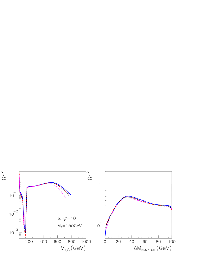
Figure 1: a) $\Omega h^{2}$ for $M_{0}=150$ GeV, $\tan\beta=10$, $A_{0}=0$, $\mu>0$ for SOFTSUSY1.8.3 (full), Isajet7.69 (dashed), Suspect2.2 (dash-dotted), and SPHENO2.20 (dotted). At large $M_{1/2}$, Isajet7.69 and Suspect2.2 give nearly identical results. b) $\Omega h^{2}$ vs $m_{\tilde{\tau}_{1}}-m_{\tilde{\chi}_{1}^{0}}$ for the same set of parameters as a).

As one moves up in $M_{1/2}$, one reaches the so-called coannihilation region where the $\tilde{\tau}$ is the NLSP and is nearly degenerate with the neutralino, as in Fig. 1b. Coannihilation with the $\tilde{\tau}$, and to a lesser extent the selectron and smuon, brings the relic density in the desired range. For a given value of $M_{1/2}$, differences between the codes can reach a factor 2, the largest differences are found between SPHENO2.20 and SOFTSUSY1.8.3. However very good agreement is found between all codes when the relic density is plotted as a function of the mass difference between the LSP and the NLSP (here the $\tilde{\tau}$). All codes obtain values of $\Omega h^{2}$compatible with WMAP for mass differences $m_{\tilde{\tau}_{1}}-m_{\tilde{\chi}_{1}^{0}}\approx 4$ GeV (at the extreme left of Fig. 1b), even though the corresponding value of the neutralino mass can differ. The value of $M_{1/2}$ for which the relic density becomes compatible with WMAP varies from 670 GeV (SPHENO2.20) to 790 GeV (SOFTSUSY1.8.3), a 12% difference on $M_{1/2}$.

3.2 Focus point
$M_{1/2}=300$ GeV, $A_{0}=0$, $\tan\beta=10$, $\mu>0$

In addition to the small $M_{0}$ (bulk/coannihilation region) where annihilation into leptons is important, the cosmologically relevant region is found at values of $M_{0}$ well above $1$TeV. As one approaches the region where electroweak symmetry breaking is forbidden, the $\mu$ parameter approaches zero. This means that the LSP is mainly Higgsino. This LSP can then annihilate very efficiently into gauge bosons (WW/ZZ) and to a lesser extent into $Zh$. The parameter $\mu$ is however very sensitive [34] to the top Yukawa coupling, $h_{t}$ (which is also reflected in a sensitivity to the value of the top quark mass) and huge differences between codes were observed[31]. The impact on the relic density and on the exclusion region is likewise very significant.

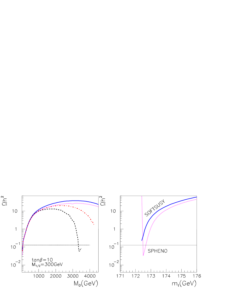
Figure 2: a) $\Omega h^{2}$ as a function of $M_{0}$ for $M_{1/2}=300$ GeV, $\tan\beta=10$, $A_{0}=0$ and $\mu>0$ and $m_{t}=175$. Same labels as in Fig. 1. b) Dependence of the relic density on $m_{t}$ for SOFTSUSY1.8.3 (full) and SPHENO2.20 (dash) .

As can be seen in Fig. 2, all codes agree very well for $M_{0}<1$TeV but as one gets to large values of $M_{0}$, more than one order of magnitude differences in $\Omega h^{2}$  can be found. For $m_{t}=175$ GeV, only Isajet finds a large drop in the $\mu$ parameter as one moves to $M_{0}\approx 3000$ GeV, this is when $\Omega h^{2}$ drops below the upper limit from WMAP. The other codes do not find this drop in $\mu$ and do not obtain a cosmologically interesting region for $M_{0}<4000$ GeV. These large differences between codes however are just a reflection of the sensitivity to the top Yukawa, $h_{t}(M_{SUSY})$ which is proportional to $m_{t}$. We show in Fig. 2b, the variation of $\Omega h^{2}$ with $m_{t}$ using SOFTSUSY1.8.3 and SPHENO2.20 for $M_{0}=3000$ GeV. The value $\Omega h^{2}=.128$ found in Isajet7.69 for $m_{t}=175$ GeV can be reproduced in SOFTSUSY1.8.3 (SPHENO) by changing the input to $m_{t}=172.2(172.5)$ GeV.

3.3 Large $\tan\beta$
$m_{1/2}=1500$ GeV, $A_{0}=0$,$\tan\beta=52$ $\mu>0$

At large $\tan\beta$ the new feature is the annihilation of neutralinos into $b\overline{b}$ via heavy Higgs exchange. With the current version of the RGE codes, this is observed only for very large values of $\tan\beta$. The crucial parameter here is $M_{A}/2m_{\tilde{\chi}_{1}^{0}}$ which must be close to unity to provide sufficient annihilation of neutralinos. Large differences in the value of $M_{A}$ between the different RGE codes occur because of the sensitivity of the RGE to the bottom Yukawa as well as from taking into account higher loop effects.

As Fig. 3a shows, all 4 programs predict a large drop in the relic density when the neutralino mass gets close to $M_{A}/2$ although this drop occurs at much lower values of $M_{1/2}$ for SPHENO, $M_{1/2}\approx 1250$ GeV than for Isajet7.69 , $M_{1/2}\approx 1750$ GeV. However, here again the results are very sensitive to the input parameters, in this case the value of the b-quark mass. For $M_{1/2}=1300$ GeV, we find an order of magnitude shift in $\Omega h^{2}$ for $m_{b}(m_{b})=4-4.4$ GeV with the program SOFTSUSY1.8.3. By a slight shift of the b-quark mass we can find perfect agreement between SPHENO2.20 and SOFTSUSY1.8.3, as shown in Fig. 3b.

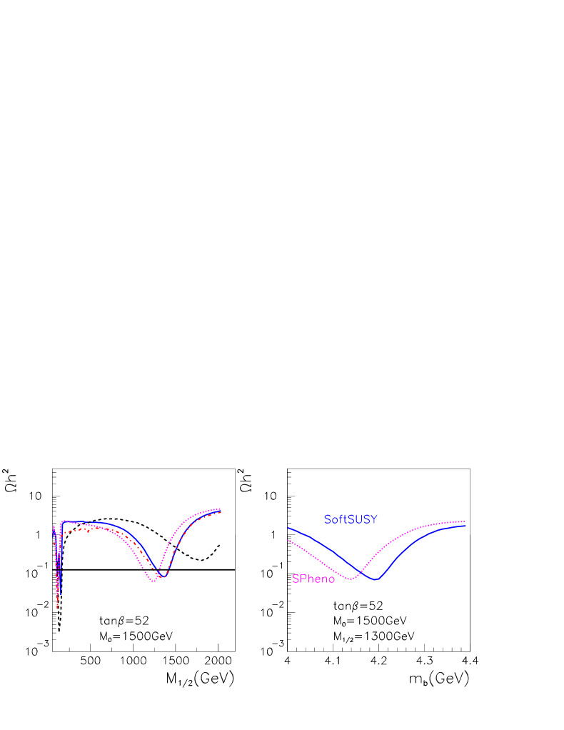
Figure 3: a) $\Omega h^{2}$ as a function of $M_{1/2}$ for $m_{t}=175$, $\tan\beta=52$, $A_{0}=0$ and $\mu>0$. Same labels as in Fig. 1. b) Dependence of the relic density on $m_{b}(m_{b})$ for SOFTSUSY1.8.3 (full) and SPHENO2.20 (dash).

4 CONCLUSION

While the predictions for the relic density of neutralinos are rather stable in most of the mSUGRA space, it is in the most physically interesting region that large discrepancies can be observed, in particular the focus point/large $\tan\beta$ and coannihilation regions. It is however reassuring to find that with the newer versions of the codes, the discrepancies in the sparticle spectra tend to be reduced. More details on the theoretical uncertainties in the evaluation of the relic density arising from the standard model parameters, $\alpha_{s},m_{b},m_{t}$, used as input in a RGE code can be found in [35].

ACKNOWLEDGEMENTS

This work was partially supported by CNRS/PiCS-397, Calculs automatiques de diagrammes de Feynman. We thank Jean-Loic Kneur for providing an improved version of Suspect2.2 .

Part V SFITTER: A Tool To Determine Supersymmetric Parameters

R. Lafaye, T. Plehn, D. Zerwas

1 Introduction

The most important task for the LHC as well as for any future Linear Collider is to study in detail the mechanism which leads to electroweak symmetry breaking. While the Standard Model describes all available high energy physics experiments, it still has to be regarded as an effective theory, valid at the weak scale. New physics are expected to appear at the TeV energy scale. The minimal supersymmetric extension of the Standard Model (MSSM) can provide a description of physics up to the unification scale.

If supersymmetry or any other high-scale extension of the Standard Model is discovered, it will be crucial to determine its fundamental high-scale parameters from weak-scale measurements [36, 37]. The LHC and a future Linear Collider will provide a wealth of measurements [38], which due to their complexity require a proper treatment to unravel the corresponding high-scale physics. Even in the general weak-scale MSSM without any unification or SUSY breaking assumptions the measurements of masses and couplings are not likely to be independend measurements; moreover, linking supersymmetric particle masses to weak-scale SUSY parameters involves non-trivial mixing to mass eigenstates in essentially every sector of the theory. On top of that, for example in gravity mediated SUSY breaking scenarios (mSUGRA/cMSSM) a given weak-scale SUSY parameter will always be sensitive to several high-scale parameters which contribute through renormalization group running. Therefore, a fit of the model parameters using all experimental information available will lead to the best sensitivity and make the most efficient use of the information available.

If the starting point of the fit is not known and many parameters are involved, the allowed parameter space might not be sampled completely in the fit approach. To avoid boundaries imposed by non-physical parameter points, which can confine the fit to a ‘wrong’ parameter region, combining the fit with an initial evaluation of a multi-dimensional grid is the optimal approach. In the general MSSM the weak-scale parameters can vastly outnumber the collider measurements, so that a complete parameter fit is not possible and one has to limit oneselve to a subset of parameters. In SFITTER both grid and fit are realised and can be combined, including a general correlation matrix and the option to exclude parameters of the model from the fit/grid by fixing them to a value.

2 SFITTER — Program Structure

Currently, SFITTER uses the predictions for the supersymmetric masses provided by SUSPECT [3], but the conventions of the SUSY Les Houches accord [19] could be helpful, if provided as a common block/C-structure, to ease interfacing other programs. The branching ratios and $e^{+}$e^- production cross sections are provided by MSMlib [39], which has been used extensively at LEP and cross checked with Ref. [40]. The next-to-leading order hadron collider cross sections are computed using PROSPINO [41, 42, 43]. The fitting program uses the MINUIT package [44]. The determination of $\chi^{2}$ includes a general correlation matrix between measurements. For unphysical points in supersymmetric parameter space, $\chi^{2}$ is set to 10³⁰.

2.1 Initialization and Steering

The program SFITTER is driven by two files: the first one sets up the measurements and the corresponding errors. For each measurement one specifies if it is to be used in the grid (G) or in the MINUIT fit (M) or in both.

//set all errors to 0.5% of their central value
DATA_ERR = 0.005
//randomize the measurements around their nominal value
RANDOMIZE = 1
//Higgs mass and error to be used in the Fit only
m_h      = 112.6 +/- 0.1 [-/M]
//Neutralino1 mass to be used in Grid and Fit
m_chi0_1 = 180.2 +/- 5.1 [G/M]
//Correlation between two chargino mass measurements
CORR(m_chi+_1,m_chi+_2) = 0.03

The second file initializes everything related to the weak-scale or high-scale MSSM model parameters. First the model (mSUGRA, pMSSM etc) is specified, then the starting values of all MSSM parameters, boundaries, stepsize and the number of points in the grid are specified. Moreover, the user defines if a certain MSSM model parameter is included in the grid and in the fit:

MODEL=MSUGRA    // use MSUGRA
// use the GRID (or not)
GRID=1
// M0 used in grid and fit, grid of 10+1 steps between 0 and 1000.
M0=500. [M/G] STEP=200. LOW=0. HIGH=1000. GRID=10
// A0 used only in fit
A0=0. [M/-] STEP=200. LOW=-1000. HIGH=1000.

2.2 mSUGRA/cMSSM Parameter Determination

Assuming that SUSY breaking is mediated by gravitational interactions (mSUGRA/cMSSM) we fit four universal high-scale parameters to a toy set of collider measurements: the universal scalar and gaugino masses, $m_{0}$, $m_{1/2}$, the trilinear coupling $A_{0}$ and the ratio of the Higgs vacuum expectation values, $\tan\beta$. The sign of the Higgsino mass parameter $\mu$ is a discrete parameter and therefore fixed. The assumed data set is the set of all supersymmetric particle masses for the SUSY parameter point SPS1a [30, 45], as computed by SUSPECT. The errors on the toy mass measurements are uniformly set to 0.5%. The starting points for the mSUGRA parameters are fixed to the mean of the lower and upper limit in the fit, i.e. they are not necessarily even close to the true SPS1a values. The result of the fit is shown in Tab. 1. With SFITTER the true parameter values were reconstructed well within the quoted errors, in spite of starting values relatively far away from the true ones. The measurement of $m_{0}$ and $m_{1/2}$ is very precise, while the sensitivity of the masses on $\tan\beta$ and $A_{0}$ is significantly weaker.

The correlations between the different high-scale SUSY parameters are also given in Tab. 1. One can understand the correlation matrix step by step [46]: first, the universal gaugino mass $m_{1/2}$ can be extracted very precisely from the physical gaugino masses. The determination of the universal scalar mass $m_{0}$ is dominated by the weak-scale scalar particle spectrum, but in particular the squark masses are also strongly dependent on the universal gaugino mass, because of mixing effects in the renormalization group running. Hence, a strong correlation between the $m_{0}$ and $m_{1/2}$ occurs. The universal trilinear coupling $A_{0}$ can be measured through the third generation weak-scale mass parameters $A_{b,t,\tau}$. However, the $A_{b,t,\tau}$ which appear for example in the off-diagonal elements of the scalar mass matrices, also depend on $m_{0}$ and $m_{1/2}$, so that $A_{0}$ is strongly correlated with $m_{0}$ and $m_{1/2}$.

In the SPS1a scenario, the pseudoscalar Higgs is heavy and the Higgs masses do not show a strong dependence on $\tan\beta$. Because of the large mass difference between gauginos and Higgsinos they essentially decouple, and the neutralino/chargino sector will not yield a good determination of $\tan\beta$. The stop mixing is governed by $A_{t}$, and not by $\mu/\tan\beta$, while the sbottom mixing is small altogether. Only the stau mixing is large and driven by $\mu\tan\beta$ in the off-diagonal element of the stau mass matrix. The stau mass parameters are dominated by $m_{0}$, in particular the smaller right handed stau mass. Therefore, one expects $\tan\beta$ to be strongly correlated with $m_{0}$ and less with $m_{1/2}$. The result from SFITTER as shown in Tab. 1 is in agreement with this prediction. Thus, the results obtained with SFITTER can be understood from the particular features of the SPS1a spectrum.

	True	FitStart	FitResult
$m_{0}$	100	500	100.01$\pm$0.58
$m_{1/2}$	250	500	249.99$\pm$0.31
$\tan\beta$	10	50	10.03$\pm$0.37
$A_{0}$	-100	0	-100.1$\pm$5.26

	$m_{0}$	$m_{1/2}$	$\tan\beta$	$A_{0}$
$m_{0}$	1	-0.47	0.41	0.26
$m_{1/2}$		1	-0.07	-0.30
$\tan\beta$			1	0.35
$A_{0}$				1

Table 1: Left: summary of mSUGRA fit in SPS1a: true values, starting values, fit values. As in SPS1a we fix $\mu>0$. All mass values are given in GeV. Right: the (symmetric) correlation matrix of all SUSY parameters in the mSUGRA fit.

2.3 MSSM Parameter Determination

In total 24 parameters describe the unconstrained weak-scale MSSM. They are listed in Tab. 2: $\tan\beta$ just like in mSUGRA, plus three soft SUSY breaking gaugino masses $M_{i}$, the Higgsino mass parameter $\mu$, the pseudoscalar Higgs mass $m_{A}$, the soft SUSY breaking masses for the right sfermions, $M_{\tilde{f}_{R}}$, the corresponding masses for the left doublet sfermions, $M_{\tilde{f}_{L}}$ and finally the trilinear couplings of the third generation sfermions $A_{t,b,\tau}$.

In any MSSM spectrum, in first approximation, the parameters $M_{1}$, $M_{2}$, $\mu$ and $\tan\beta$ determine the neutralino and chargino masses and couplings. We exploit this feature to illustrate the option to use a grid before the start the complete MINUIT fit. For testing purposes, the error on all mass measurements is again set 0.5%. The starting values of the parameters are set to their nominal values, this study is thus less general than the one of mSUGRA. Then we minimize $\chi^{2}$ on a grid. For this grid minimization the six chargino and neutralino masses are used as measurements to determine the four SUSY parameters $M_{1}$, $M_{2}$, $\mu$ and $\tan\beta$ only. The step size of the grid is 10 for $\tan\beta$ and 100 GeV for the three mass parameters. After the minimization, these four parameters obtained from the minimum $\chi^{2}$ on the grid are fixed and all remaining parameters are fitted. Only in a final run all SUSY parameters are released and fitted, to give the final results quoted in Tab. 2.

In Tab. 2 the intermediate (after the grid evaluation) results, the final results and the nominal values are shown. The final fit values indeed converges to the correct central values within its error. The central values of the fit are in good agreement with generated values, except for the trilinear coupling $A_{b}$. As already mentioned in the discussion of the mSUGRA fit, the mixing between the two sbottom mass states is very small, so the assumed precision of the 0.5% is insufficient to determine the parameter from the mass measurements alone. As $A_{t}$ enters in the calculation of the lightest Higgs, additional sensitivity for this parameter comes from the mass measurement of the lightest Higgs boson. The use of branching ratios and cross section measurements should significantly increase the precision in future studies, especially for $A_{\tau}$ and $A_{b}$.

	AfterGrid	AfterFit	SPS1a		AfterGrid	AfterFit	SPS1a
$\tan\beta$	10	10.62$\pm$2.5	10	$M_{\tilde{u}_{R}}$	528.03	528.06$\pm$2.8	532.1
$M_{1}$	100	102.05$\pm$0.61	102.2	$M_{\tilde{d}_{R}}$	525.12	525.14$\pm$2.8	529.3
$M_{2}$	200	191.65$\pm$1.4	191.8	$M_{\tilde{c}_{R}}$	528.03	528.06$\pm$2.8	532.1
$M_{3}$	579.37	579.33$\pm$4.8	589.4	$M_{\tilde{s}_{R}}$	525.12	525.15$\pm$2.8	529.3
$\mu$	300	344.04$\pm$1.2	344.3	$M_{\tilde{t}_{R}}$	417.36	415.44$\pm$5.7	420.2
$m_{A}$	399.38	399.14$\pm$1.2	399.1	$M_{\tilde{b}_{R}}$	524.59	523.99$\pm$2.9	525.6
$M_{\tilde{e}_{R}}$	138.24	138.23$\pm$0.76	138.2	$M_{\tilde{q}1_{L}}$	549.58	549.61$\pm$2.1	553.7
$M_{\tilde{\mu}_{R}}$	138.24	138.23$\pm$0.76	138.2	$M_{\tilde{q}2_{L}}$	549.58	549.61$\pm$2.1	553.7
$M_{\tilde{\tau}_{R}}$	135.58	135.51$\pm$2.1	135.5	$M_{\tilde{q}3_{L}}$	493.59	494.38$\pm$2.7	501.3
$M_{\tilde{e}_{L}}$	198.74	198.75$\pm$0.68	198.7	$A_{\tilde{\tau}}$	-724.25	-286.78$\pm$549	-253.5
$M_{\tilde{\mu}_{L}}$	198.74	198.75$\pm$0.68	198.7	$A_{\tilde{t}}$	-502.19	-495.19$\pm$15	-504.9
$M_{\tilde{\tau}_{L}}$	197.79	197.81$\pm$0.89	197.8	$A_{\tilde{b}}$	975.12	999.78$\pm$49	-799.4

Table 2: Result for the general MSSM parameter determination in SPS1a. Shown are the nominal parameter values, the result after the grid and the final result. The deviation in the squark sector of 1% is an artefact of differences between MSSM and mSUGRA part of the renomalization group code [3]. All masses are given in GeV.

3 Conclusions

SFITTER is a new program to determine suspersymmetric parameters from experimental measurements. The parameters can be extracted either using a fit, a multi-dimensional grid minimisation, or a combination of the two. Correlations between measurements can be specified and are taken into account in the calculation of the $\chi^{2}$. SUSPECT, MSMlib and PROSPINO are used to calculate the predictions for the masses, branching ratios and production cross sections. A more realistic set of the measurements for example assuming the SPS1a mass spectrum for the LHC and and a future Linear Collider will be studied as a next step. The impact of correlations between measurements on the estimated errors of MSSM parameters will be studied in detail. In the future public version of the program we will include different generators for the calculation of masses and branching ratios.

Acknowledgements

The authors would like to thank the organizers of the Les Houches workshop and the convenors of the BSM working-group for the constructive atmosphere in which SFITTER was born. TP would in particular like to thank Michael Spira for allowing him to participate in the Higgs and the BSM sessions at the Les Houches workshop.

Part VI SDECAY: a Code for the Decays of the Supersymmetric Particles

A. Djouadi, Y. Mambrini and M. Mühlleitner

1 Introduction

The search for new particles predicted by supersymmetric (SUSY) theories is a major goal of present and future colliders. In the Minimal Supersymmetric Standard Model (MSSM) [47] there are still over 20 free parameters even in a phenomenologically viable model. It is therefore a very complicated task to deal with all the properties of the SUSY particles once they are found. Since their properties will be determined with an accuracy of a few per cent at the LHC and a precision at the per cent level or below at future $e^{+}e^{-}$ linear colliders, the mass spectra, the various couplings, the decay branching ratios and the production cross sections have to be calculated with a rather high precision, also including higher order effects. The Fortran code SDECAY [8] which is presented here calculates the decays of SUSY particles in the MSSM, including the most important higher order effects. The Renormalization Group Equation (RGE) program SuSpect [3] is used for the calculation of the mass spectrum and the soft SUSY-breaking parameters. [Of course, SDECAY can be easily linked to any other RGE code.] Due to the limited space we refer for details of the notation, the description of the algorithm that is used in the code and the various higher order effects that have been included to the user’s manual of SuSpect. The program SDECAY then evaluates the various couplings of the SUSY particles and MSSM Higgs bosons and calculates the decay widths and the branching ratios of all the two-body decay modes, including the QCD corrections to the processes involving coloured particles and the dominant electroweak effects to all processes. The loop-induced two-body decay channels as well as the possibly important higher order decays are included, such as the three-body decays of charginos, neutralinos, gluinos and top squarks and the four-body decays of the lighter top squark. In addition, the top quark SUSY decay widths and branching ratios are implemented. The program will be presented in the following.

2 The decays of the supersymmetric particles

2.1 The tree level two-body decays

The Fortran code SDECAY includes the two-body decays of sfermions into a fermion and a gaugino, as well as into a lighter sfermion of the same isodoublet and a gauge boson $V\!=\!W,Z$ or a Higgs boson $\Phi=h,H,A,H^{\pm}$

$$\tilde{f}_{i} \to \chi_{j}f^{(^{\prime})}$$ (1)

$$\tilde{f}_{i} \to V\tilde{f}_{j}^{(^{\prime})}$$ (2)

$$\tilde{f}_{i} \to \Phi\tilde{f}_{j}^{(^{\prime})}$$ (3)

For squarks heavier than the gluino the decay into a gluino-quark final state is also possible

$$\tilde{q}_{i}\to q\tilde{g}$$ (4)

The heavier neutralino and chargino decays into the lighter chargino and neutralino states and gauge or Higgs bosons as well as the decays into fermion-sfermion pairs have been implemented

$$\chi_{i} \to \chi_{j}V$$ (5)

$$\chi_{i} \to \chi_{j}\Phi$$ (6)

$$\chi_{i} \to f\tilde{f}_{j}^{(^{\prime})}$$ (7)

For the gluinos the only relevant decay into a squark-quark pair is calculated

$$\tilde{g}\to q\tilde{q}_{i}$$ (8)

In the case of a GMSB model the decays of the next-to-lightest SUSY particle (NLSP), which can be either the lightest neutralino $\chi_{1}^{0}$ or the lightest sfermion, in general the $\tilde{\tau}_{1}$, into a Gravitino $\tilde{G}$ and a photon, $Z$ or neutral Higgs boson (for $\chi_{1}^{0}$) and a $\tau$ (for $\tilde{\tau}_{1}$) are implemented

$$\chi_{1}^{0} \to \gamma\tilde{G},Z\tilde{G},\Phi\tilde{G}$$ (9)

$$\tilde{\tau}_{1} \to \tau\tilde{G}$$ (10)

The masses entering the phase space in the calculation of the widths are the pole masses, but when they enter the various couplings they are - for the third-generation fermions - the running $\overline{{\rm DR}}$ masses at the scale of Electroweak Symmetry Breaking (EWSB). This is also the case for all soft SUSY-breaking parameters and the third generation sfermion mixing angles involved in the couplings. In addition, we have left the option for the QCD coupling constant and the bottom, top Yukawa couplings to be evaluated at the scale of the decaying superparticle or any other scale. In this case, only the standard QCD corrections are included in the running [48].

2.2 The QCD corrected two-body decays

The one-loop QCD corrections to the following two-body decays involving (s)quarks and gluinos have been implemented using the formulae of Refs. [49, 50], [51, 52, 53, 54] and [55, 56], respectively,

$$\tilde{q}_{i} \to \chi_{j}q^{(^{\prime})}$$ (11)

$$\tilde{q}_{i} \to \Phi\tilde{q}_{j}^{(^{\prime})}$$ (12)

$$\tilde{q}_{i} \to q\tilde{g}\quad{\rm and}\quad\tilde{g}\to\tilde{q}_{i}q$$ (13)

All the corrections have been included in the $\overline{{\rm DR}}$ scheme. The bulk of the electroweak radiative corrections due to the running of the gauge and third-generation fermion Yukawa couplings has been taken into account by evaluating these parameters at the EWSB scale.

2.3 Loop-induced decays

In case the two-body decays of the next-to-lightest neutralino are kinematically not allowed the loop-induced decay into the lightest supersymmetric particle (LSP) $\chi_{1}^{0}$ and a photon is calculated [57, 58, 59, 60]

$$\chi_{2}^{0}\to\chi_{1}^{0}\gamma$$ (14)

For completeness, the loop-induced decay of a gluino into a gluon and the LSP has also been considered [61, 62, 63]

$$\tilde{g}\to g\chi_{1}^{0}$$ (15)

If the tree-level stop two-body decays are kinematically closed the loop-induced decay into a charm and $\chi_{1}^{0}$ [64] is calculated

$$\tilde{t}_{i}\to c\chi_{1}^{0}$$ (16)

2.4 Multibody decay modes

If the two-body decays of the gauginos Eqs. (5-7) are kinematically forbidden the three-body decays into a lighter gaugino and a fermion pair and a gluino and two quarks are calculated

$$\chi_{i} \to \chi_{j}f\bar{f}^{(^{\prime})}$$ (17)

$$\chi_{i} \to \tilde{g}q\bar{q}^{(^{\prime})}$$ (18)

Analogously, the gluino three-body decays into a gaugino and two quarks are considered when the gluino two-body modes are closed

$$\tilde{g}\to\chi_{i}q\bar{q}^{(^{\prime})}$$ (19)

For the calculation of the processes Eqs. (17-19) we have used the formulae given in [65, 66, 67, 68, 69]. Furthermore, the possibly important gluino decay into stop, bottom and a $W$ boson as well as the decay into stop, bottom and a charged Higgs boson have been implemented [70, 71]

$$\tilde{g} \to \tilde{t}_{1}\bar{b}W^{-}$$ (20)

$$\tilde{g} \to \tilde{t}_{1}\bar{b}H^{-}$$ (21)

In case the stop two-body decays are not accessible, there are several three-body decay modes [72, 73, 74, 75, 76, 77] that can dominate over the loop-induced decay Eq. (16) in rather large areas of the MSSM: the decays into a bottom, lightest neutralino and a $W$ or charged Higgs boson, the decay modes into bottom, lepton and slepton, the decays into the lightest sbottom and a fermion pair as well as for the heavy stop the possibility of decaying into the lighter stop and a fermion pair

$$\tilde{t}_{i} \to bW^{+}\chi_{1}^{0}\quad,\quad\quad\;\;bH^{+}\chi_{1}^{0}$$ (22)

$$\tilde{t}_{i} \to bl^{+}\tilde{\nu}_{l}\quad{\rm and/or}\quad b\tilde{l}^{+}\nu_{l}$$ (23)

$$\tilde{t}_{i} \to \tilde{b}_{1}f\bar{f}^{\prime}$$ (24)

$$\tilde{t}_{2} \to \tilde{t}_{1}f\bar{f}$$ (25)

SDECAY evaluates the three-body decays if the two-body decays are closed, taking into account all possible contributions of virtual particles, the radiatively corrected Yukawa couplings of third-generation fermions, the mixing pattern for their sfermion partners and the masses of the sparticles and gauge/Higgs bosons involved in the processes. Even the masses of the final state fermions have been included. The total decay widths of the exchanged particles have not been included in the propagators of the virtual particles.

If the stop three-body decay channels are kinematically forbidden the $\tilde{t}_{1}$ four-body decay mode into a bottom, the LSP and two massless fermions can become competitive with the loop induced decay into a charm and a neutralino, cf. Eq. (16), so that this channel [78] has also been included in the program,

$$\tilde{t}_{1}\to b\chi_{1}^{0}f\bar{f}^{\prime}$$ (26)

2.5 Top quark decays

For the top quark the following decays in the MSSM are calculated by SDECAY

$$t \to bW^{+}$$ (27)

$$t \to bH^{+}\quad{\rm and}\quad\tilde{t}_{1}\chi_{1}^{0}$$ (28)

3 How to use SDECAY

Apart from the files of the program SuSpect, i.e. suspect2.in, suspect2.f, subh_hdec.f, feynhiggs.f, hmsusy.f, the program SDECAY consists of three files:
h 1) The input file sdecay.in where one can choose the accuracy of the algorithm and the various options whether QCD corrections and multibody or loop decays are included or not, which scales and how many loops are used for the running couplings and if top and GMSB decays are calculated or not.
h 2) The main routine sdecay.f where the couplings of the SUSY and Higgs particles are evaluated and the decay branching ratios and total widths are calculated.
h 3) The output file sdecay.out which gives the results for the branching ratios and total widths, as well as the masses of the SUSY and Higgs particles, the mixing matrices and the gauge and third-generation Yukawa couplings at the EWSB or a chosen scale. The output is given in two possible formats, either in a simple and transparent form or according to the SUSY Les Houches Accord [19] which uses the PDG notation for the particles.
All these files together with a makefile to compile the files can be found on the web page dedicated to SDECAY at the address:

http://people.web.psi.ch/muehlleitner/SDECAY

4 Conclusions

We have presented the Fortran code SDECAY, which calculates the decay widths and branching ratios of all the two-body decays of the SUSY particles in the framework of the MSSM, including the QCD corrections to the decays involving strongly interacting particles, the three-body decays of the gauginos, gluinos and stops, as well as the four-body decays of the lightest top squark. Furthermore, the loop-induced decays of the gluino, the lightest neutralino and the lightest top squark, the decays of the next-to-lightest SUSY particle in GMSB models and the standard and SUSY decay modes of the top quark have been implemented. The dominant electroweak corrections due to the running of the gauge and fermion Yukawa couplings have been incorporated. The program which uses the RGE code SuSpect can be easily linked to any other spectrum calculator. It is user-friendly, flexible for the choice of options and approximations and quite fast. The program is under rapid development and will be updated regularly.

Part VII Measuring The Mass Of The Lightest Chargino At The CERN LHC

M.M. Nojiri, G. Polesello and D.R. Tovey

1 INTRODUCTION

Much work has been carried out recently on measurement of the masses of SUSY particles at the LHC [79, 80, 81, 82, 83, 84]. These measurements can often be considered to be ‘model-independent’ in the sense that they require only that a particular SUSY decay chain exists with an observable branching ratio. A good starting point is often provided by the observation of an opposite-sign same-flavour (OS-SF) dilepton invariant mass spectrum end-point whose position measures a combination of the masses of the $\tilde{\chi}^{0}_{2}$, the $\tilde{\chi}^{0}_{1}$ and possibly also the $\tilde{l}^{\pm}$. Observation of end-points and thresholds in invariant mass combinations of some or all of these leptons with additional jets then provides additional mass constraints sufficient to allow the individual sparticle masses to be reconstructed unambiguously. A question remains however regarding how the mass of a SUSY particle can be measured if it does not participate in a decay chain producing an OS-SF dilepton signature. This problem has been addressed for some sparticles (e.g. for the $\tilde{q}_{R}$ [85]) however significant exceptions remain. Notable among these is the case of the lightest chargino $\tilde{\chi}^{\pm}_{1}$, which does not usually participate in decay chains producing OS-SF dileptons due to its similarity in mass to the $\tilde{\chi}^{0}_{2}$.

In this paper we attempt to measure the mass of the $\tilde{\chi}^{\pm}_{1}$ by identifying the usual OS-SF dilepton invariant mass end-point arising from the decay via $\tilde{\chi}^{0}_{2}$ of the other initially produced SUSY particle (i.e. not the one which decays to produce the $\tilde{\chi}^{\pm}_{1}$). We then solve the mass constraints for that decay chain to reconstruct the momentum of the $\tilde{\chi}^{0}_{1}$ appearing at the end of the chain, and use this to constrain the momentum (via $E_{T}^{miss}$) of the $\tilde{\chi}^{0}_{1}$ appearing at the end of the decay chain involving the $\tilde{\chi}^{\pm}_{1}$. We finally use mass constraints provided by additional jets generated by this chain to solve for the $\tilde{\chi}^{\pm}_{1}$ mass. The technique requires that both the decay chain

$$\tilde{q}_{L}\rightarrow\tilde{\chi}^{0}_{2}q\rightarrow\tilde{l}_{R}lq\rightarrow\tilde{\chi}^{0}_{1}llq$$

and the decay chain

$$\tilde{q}_{L}\rightarrow\tilde{\chi}^{\pm}_{1}q\rightarrow qW^{\pm}\tilde{\chi}^{0}_{1}\rightarrow qq^{\prime}q^{\prime\prime}\tilde{\chi}^{0}_{1}$$

are open with significant branching ratios, and that the masses of the $\tilde{\chi}^{0}_{1}$, $\tilde{\chi}^{0}_{2}$, $\tilde{l}_{R}$ and $\tilde{q}_{L}$ are known. No other model-dependent assumptions are required however.

2 SUSY MODEL AND EVENT GENERATION

The SUSY model point chosen was that used recently by ATLAS for full simulation studies of SUSY mass reconstruction [86]. This is a minimal Supergravity (mSUGRA) model with parameters $m_{0}$ = 100 GeV, $m_{1/2}$ = 300 GeV, $A_{0}$ = -300 GeV, $\tan(\beta)$ = 6 and $\mu>0$. The mass of the lightest chargino is 218 GeV, while those of the $\tilde{q}_{L}$, the $\tilde{l}_{R}$, the $\tilde{\chi}^{0}_{2}$ and the $\tilde{\chi}^{0}_{1}$ are $\sim$ 630 GeV, 155 GeV, 218 GeV and 118 GeV respectively. One of the characteristics of this model is that the branching ratio of $\tilde{\chi}^{\pm}_{1}\rightarrow W^{\pm}\tilde{\chi}^{0}_{1}$ is relatively large ($\sim$ 28 %). Chargino mass reconstruction involving the decay $\tilde{\chi}^{\pm}_{1}\rightarrow\tilde{\tau}_{1}\nu_{\tau}$ (BR $\sim$ 68 %) is likely to be very difficult due to the additional degress of freedom provided by the missing neutrino. Consequently the $W^{\pm}$ decay mode must be used.

The electroweak SUSY parameters were calculated using the ISASUGRA 7.51 RGE code [11]. SUSY events equivalent to an integrated luminosity of 100 fb^-1 were then generated using Herwig 6.4 [12, 87] interfaced to the ATLAS fast detector simulation ATLFAST 2.21 [88]. With the standard SUSY selection cuts described below Standard Model backgrounds are expected to be negligible. An event pre-selection requiring at least two ATLFAST-identified isolated leptons was applied in order to reduce the total volume of data.

3 CHARGINO MASS RECONSTRUCTION

Events were required to satisfy ‘standard’ SUSY selection criteria requiring a high multiplicity of high $p_{T}$ jets, large $E_{T}^{miss}$ and multiple leptons:

• at least 4 jets (default ATLFAST definition [88]) with $p_{T}$ $>$ 10 GeV, two of which must have $p_{T}$ $>$ 100 GeV,

• $\left(\sum_{i=1}^{4}p_{T(jet)}^{i}+E_{T}^{miss}\right)$ $>$ 400 GeV,

• $E_{T}^{miss}$ $>$ max$\left(100\mathrm{GeV},0.2\left(\sum_{i=1}^{4}p_{T(jet)}^{i}+E_{T}^{miss}\right)\right)$,

• exactly 2 opposite sign same flavour isolated electrons or muons with $p_{T}$ $>$ 10 GeV,

• no b-jets or $\tau$-jets.

Events were further required to contain dileptons with an invariant mass less than the expected $l^{\pm}l^{\mp}$ end-point position (100.2 GeV) and at least one dilepton + hard jet combination (one for each combination of the dilepton pair with each of the two hardest jets) with an invariant mass less than the expected $l^{\pm}l^{\mp}q$ end-point position (501.0 GeV). The smaller dilepton + hard jet combination then defined which jet (assumed to be from the decay $\tilde{q}_{L}\rightarrow\tilde{\chi}^{0}_{2}q$) would be used together with the dileptons to reconstruct the $\tilde{\chi}^{0}_{2}$ production and decay chain.

The momentum of the $\tilde{\chi}^{0}_{1}$ at the end of the $\tilde{\chi}^{0}_{2}$ decay chain was calculated by solving analytically the kinematic equations relating the momenta of the decay products (including the $\tilde{\chi}^{0}_{1}$) to the masses of the SUSY particles, which were assumed to be known from conventional end-point measurements [79, 80, 81, 82, 83, 84]. This process is described in more detail in Ref. [89] and results in two solutions for the $\tilde{\chi}^{0}_{1}$ momentum for each of the two possible mappings of the reconstructed leptons to the sparticle decay products. In the present analysis just one such mapping was assumed with no attempt being made to select the correct assignment. Two possible solutions for the $\tilde{\chi}^{0}_{1}$ momentum were therefore obtained for each event.

Figure 1: Reconstructed dijet invariant mass distributions for all events (data points) and events not containing the decay chain $\tilde{\chi}^{\pm}_{1}\rightarrow W^{\pm}\tilde{\chi}^{0}_{1}\rightarrow q^{\prime}q^{\prime\prime}\tilde{\chi}^{0}_{1}$ selected using Monte Carlo truth. The signal band is labelled ‘I’ in the figure, while the two sideband are labelled ‘II’ and ‘III’ respectively.

The nest step in the reconstruction was to find the jet pair resulting from a hadronic $W^{\pm}$ decay following production via $\tilde{\chi}^{\pm}_{1}\rightarrow W^{\pm}\tilde{\chi}^{0}_{1}$. The potentially large combinatorial background was reduced by rejecting jet combinations involving either of the two hardest jets (since these were assumed to arise from $\tilde{q}_{L}$ decay) and by requiring that the harder(smaller) of the two jets possessed $p_{T}$ greater than 40(20) GeV (i.e. selecting asymmetric jet pairs consistent with a significant boost in the lab frame). A further cut was applied on the invariant mass of the combination of the jet pair with the hard jet giving the larger dilepton + jet mass (assumed therefore to be the jet from the $\tilde{q}_{L}\rightarrow\tilde{\chi}^{\pm}_{1}q$ decay preocess). This invariant mass was conservatively required to be less than that of the $\tilde{q}_{L}$.

For each event any jet pairs satisfying the above criteria and possessing $|m_{jj}-m_{W}|$ $<$ 15 GeV (Fig. 1), were considered to form $W$ candidates. For each event the candidate with $m_{jj}$ nearest $m_{W}$ was then selected and used together with the momentum of the hard jet identified previously and the two assumed $x$ and $y$ components of the $\tilde{\chi}^{0}_{1}$ momentum (calculated from the two solutions for the momentum of the $\tilde{\chi}^{0}_{1}$ from the $\tilde{\chi}^{0}_{2}$ decay and $E_{T}^{miss}$) to calculate the chargino mass. Each of the two solutions for the $\tilde{\chi}^{0}_{1}$ momentum gives two possible solutions for $m_{\tilde{\chi}^{\pm}_{1}}$, the smaller of which is usually physical. Consequently two possible values for $m_{\tilde{\chi}^{\pm}_{1}}$ were obtained from each event (plotted in Fig. 2).

Figure 2: Reconstructed $\tilde{\chi}^{\pm}_{1}$ mass distributions showing signal distributions with $|m_{jj}-m_{W}|$ $<$ 15 GeV (data points) and sideband distributions with 15 GeV $<$ $|m_{jj}-m_{W}|$ $<$ 45 GeV (histograms). The left hand figure was obtained by selecting events containing the decay chain $\tilde{\chi}^{\pm}_{1}\rightarrow W^{\pm}\tilde{\chi}^{0}_{1}\rightarrow q^{\prime}q^{\prime\prime}\tilde{\chi}^{0}_{1}$ using Monte Carlo truth. The central figure was obtained by selecting background events not containing this decay chain. The right hand figure was obtained by using all data.

Following this procedure significant backgrounds remain from combinatorics in SUSY signal events (due to their high average multiplicity), and from SUSY background events (i.e. events in which the decay process $\tilde{q}_{L}\rightarrow\tilde{\chi}^{\pm}_{1}q\rightarrow qW^{\pm}\tilde{\chi}^{0}_{1}\rightarrow qq^{\prime}q^{\prime\prime}\tilde{\chi}^{0}_{1}$ is not present). These backgrounds (or at least those not involving a real $W^{\pm}$ decay) were removed statistically using a sideband subtraction technique similar to that described in Ref. [90]. All jet pairs satisfying all the above selection criteria except the $|m_{jj}-m_{W}|$ requirement were recorded if they satisfied the alternative requirement that 15 GeV $<$ $|m_{jj}-m_{W}|$ $<$ 45 GeV. This requirement then defined two side-bands located on either side of the main signal band ($|m_{jj}-m_{W}|$ $<$ 15 GeV) of equal width 30 GeV. The momentum of each jet pair was then rescaled such that the difference between its rescaled mass and $m_{W}$ was the same as the difference between its original mass and the centre of its sideband (50 or 110 GeV respectively). Each jet pair was then given a weight of 1.3 (lower sideband) or 1.0 (upper sideband) to account for the variation of the background $m_{jj}$ distribution with $m_{jj}$ (Fig. 1). Values for the chargino mass were then calculated for each jet pair and used to create a sideband mass distribution (Fig. 2). Finally the sideband mass distribution was subtracted from the signal mass distribution with a relative normalisation factor of 0.7 to account for the differing efficiencies for selecting sideband events and background events in the signal region.

4 RESULTS

Figure 3: Reconstructed $\tilde{\chi}^{\pm}_{1}$ mass distribution for $\tilde{\chi}^{\pm}_{1}\rightarrow W^{\pm}\tilde{\chi}^{0}_{1}\rightarrow q^{\prime}q^{\prime\prime}\tilde{\chi}^{0}_{1}$ signal events (histogram) and all events (points with errors).

The sideband subtracted chargino mass distributions obtained from this process are shown in Fig. 3, both with and without a selection requirement for $\tilde{\chi}^{\pm}_{1}\rightarrow W^{\pm}\tilde{\chi}^{0}_{1}\rightarrow q^{\prime}q^{\prime\prime}\tilde{\chi}^{0}_{1}$ obtained from Monte Carlo truth. In both cases no events are observed at masses below the kinematic limit of 198 GeV ($=m_{W}+m_{\tilde{\chi}^{0}_{1}}$) due to the origin of the mass values as solutions to the kinematic mass relations. In the case where Monte Carlo truth was used as input a clear peak is seen in the 200 GeV - 250 GeV bin, corresponding well to the actual mass of 218 GeV. At higher mass values the sideband subtraction process has worked well and the distribution is consistent with zero. In the case where no Monte Carlo truth signal event selection has been performed (points with errors) a clear peak is again seen in the vicinity of the chargino mass, with few events at higher values. For 100 fb^-1 the statistical significance of the peak is around 3 $\sigma$ indicating that more integrated luminosity (or an improved event selection) would be required to claim a 5 $\sigma$ discovery. Nevertheless it seems reasonable to claim that if this data were generated by an LHC experiment such as ATLAS, and that the observed signal were indeed not a statistical fluctuation, then the mass of the lightest chargino could be measured to a statistical precision $\sim$ $\pm$ 25 GeV ($\sim$ 11 %). More work is needed to determine the likely systematic error in this quantity arising from effects such as the statistical and systematic uncertainty in the input sparticle masses used when calculating the $\tilde{\chi}^{0}_{1}$ momentum and $\tilde{\chi}^{\pm}_{1}$ mass.

More work is needed to identify the optimum set of selection criteria required to identify hadronic $W^{\pm}$ decays in this sample, with the efficiency of the tau veto (required to remove $\tilde{\chi}^{\pm}_{1}$ decays via $\tilde{\tau}_{1}\nu_{\tau}$) in particular needing to be optimised. Possible methods for selecting the correct lepton mapping used to calculate the $\tilde{\chi}^{0}_{1}$ momentum also deserve further study. With these improvements and/or more integrated luminosity it should then be possible both to increase the accuracy of the chargino mass measurement and to study quantities such as the helicity of the $\tilde{\chi}^{\pm}_{1}$ through measurement of the invariant mass distribution of the $W^{\pm}$ and the hard jet produced alongside the $\tilde{\chi}^{\pm}_{1}$ in the decay of the parent $\tilde{q}_{L}$.

5 CONCLUSIONS

A study of the identification and measurement of charginos decaying to $W^{\pm}\tilde{\chi}^{0}_{1}$ produced at the LHC has been performed. The results indicate that for one particular mSUGRA model the mass of the $\tilde{\chi}^{\pm}_{1}$ can be measured with a statistical precision $\sim$ 11 % for 100 fb^-1 of integrated luminosity.

ACKNOWLEDGEMENTS

This work was performed in the framework of the workshop: Les Houches 2003: Physics at TeV Scale Colliders. We wish to thank the staff and organisers for all their hard work before, during and after the workshop. We thank members of the ATLAS Collaboration for helpful discussions. We have made use of ATLAS physics analysis and simulation tools which are the result of collaboration-wide efforts. DRT wishes to acknowledge PPARC and the University of Sheffield for support.

Part VIII Chargino/Neutralino Sector In Combined Analyses At LHC/LC

K. Desch, J. Kalinowski, G. Moortgat-Pick, M.M. Nojiri and G. Polesello

1 INTRODUCTION

The unconstrained MSSM has 105 new parameters and SUSY analyses at future experiments, at the LHC and at a future Linear Collider (LC), will have to focus on the determination of these parameters [91, 92]. An interesting possibility to explore SUSY is to start with the gaugino/higgsino particles which are expected to be among the lightest SUSY particles. At tree level, this sector depends only on 4 parameters: $M_{1}$, $M_{2}$, $\mu$ and $\tan\beta$ – the U(1) and SU(2) gaugino masses, the higgsino mass parameter and the ratio of the vacuum expectations of the two Higgs fields, respectively.

Some strategies have been worked out for the determination of the parameters $M_{2}$, $M_{1}$, $\mu$, $\tan\beta$ even if only the light gaugino/higgsino particles, $\tilde{\chi}^{0}_{1}$, $\tilde{\chi}^{0}_{2}$ and $\tilde{\chi}^{\pm}_{1}$ were kinematically accessible at the first stage of the LC [93, 94]. In this contribution we demonstrate how such an LC analysis could be strengthened if in addition some information on the mass of the heaviest neutralino from the LHC is available. We consider the cases: (i) stand alone LC data and (ii) joint analysis of the LC and the LHC data. The results in the last scenario will clearly demonstrate the essentiality of the LHC and LC and the benefit from the joint analysis of their data.

We take the SPS1a as a working benchmark [30, 45] and assume that only the first phase of a LC with a tunable energy up to $\sqrt{s}=500$ GeV would overlap with the LHC running. Furthermore, we assume an integrated luminosity of $\int{\cal L}\sim 500$ fb^-1 and polarised beams with $P(e^{-})=\pm 80\%$, $P(e^{+})=\pm 60\%$. In the following $\sigma_{L}$ will refer to cross sections obtained with $P(e^{-})=-80\%$, $P(e^{+})=+60\%$, and $\sigma_{R}$ with $P(e^{-})=+80\%$, $P(e^{+})=-60\%$.

2 THE GAUGINO/HIGGSINO SECTOR

The mass matrix ${\cal M}_{C}$ of the charged gaugino $\tilde{W}^{\pm}$ and higgsino $\tilde{H}^{\pm}$ depends on $M_{2}$, $\mu$, $\tan\beta$. The mass eigenstates are the two charginos $\tilde{\chi}^{\pm}_{1,2}$. For real ${\cal M}_{C}$ the two unitary diagonalisation matrices can be parameterised with two mixing angles $\Phi_{L,R}$. The mass eigenvalues $m^{2}_{\tilde{\chi}^{\pm}_{1,2}}$ and the mixing angles are analytically given by the Susy parameters (see e.g. [95, 96]). The cross section $\sigma^{\pm}\{ij\}=\sigma(e^{+}e^{-}\to\tilde{\chi}^{\pm}_{i}\tilde{\chi}^{\mp}_{j})$ can be expressed as a function of $(\cos 2\Phi_{L,R},m^{2}_{\tilde{\chi}^{\pm}_{i}})$; the coefficients for $\sigma^{\pm}\{11\}$ are explicitly given in [97].

The neutralino mixing matrix ${\cal M}_{N}$ depends on $M_{1}$, $M_{2}$, $\mu$ and $\tan\beta$. Analytic expressions for the mass eigenvalues $m^{2}_{\tilde{\chi}^{0}_{1,\ldots,4}}$ and the eigenvectors are e.g. given in [93, 94]. The characteristic equation of the mass matrix squared, ${\cal M}_{N}{\cal M}^{\dagger}_{N}$, is written explicitly as a quadratic equation for the parameter $M_{1}$ [97].

3 STRATEGY FOR THE DETERMINATION OF THE SUSY PARAMETERS

At the initial phase of future $e^{+}e^{-}$ linear–collider operations with polarised beams, the collision energy may only be sufficient to reach the production thresholds of the light chargino $\tilde{\chi}^{\pm}_{1}$ and the two lightest neutralinos $\tilde{\chi}^{0}_{1},\,\tilde{\chi}^{0}_{2}$. Nevertheless the entire tree level structure of the gaugino/higgsino sector can be unraveled [93, 94, 95].

Chargino cross sections measured at $\sqrt{s}=400$ GeV and 500 GeV with polarised beams and the lightest chargino mass are sufficient to determine unambiguously the mixing angles $\cos 2\Phi_{L,R}$. Then the $M_{1}$ can be obtained from the quadratic equation ${\cal M}_{N}{\cal M}^{\dagger}_{N}$. However, using the kinematically accessible cross sections for the neutralino production $\sigma^{0}_{L,R}\{12\}$ and $\sigma^{0}_{L,R}\{22\}$ leads to a precise determination of the fundamental Susy parameters [97].

In the following we perform this strategy for the benchmark scenario SPS1a [30, 45] defined at the electroweak scale: $M_{1}=99.13\leavevmode\nobreak\ \mbox{GeV}$, $M_{2}=192.7\leavevmode\nobreak\ \mbox{GeV}$, $\mu=352.4\leavevmode\nobreak\ \mbox{GeV}$, $\tan\beta=10$; the resulting masses are given in table 1.

3.1 SUSY PARAMETERS FROM THE LC DATA

We use the light chargino and neutralino masses $m_{\tilde{\chi}^{\pm}_{1}}$, $m_{\tilde{\chi}^{0}_{1,2}}$ and the polarised cross sections for the processes $e^{+}e^{-}\to\tilde{\chi}^{+}_{1}\tilde{\chi}^{-}_{1}$, $\tilde{\chi}^{0}_{1}\tilde{\chi}^{0}_{2}$, $\tilde{\chi}^{0}_{2}\tilde{\chi}^{0}_{2}$ at $\sqrt{s}=400$, $500$ GeV as experimental input.

In our scenario the light chargino $\tilde{\chi}^{\pm}_{1}$ and also the neutralino $\tilde{\chi}^{0}_{2}$ decay mainly via $\tilde{\tau}_{1}$ chains producing the final states similar to that of stau pair production, however with different topology. Therefore, we assume that the contamination of stau production events can be subtracted from the chargino and neutralino production [97].

In our analysis we take the production cross sections with statistical errors induced by the following uncertainties:

• The chargino mass measurement has been simulated and the expected error is 0.55 GeV, see table 1.

• With $\int{\cal L}=500$ fb^-1 at the LC, we assume 100 fb^-1 per each polarisation configuration and we take into account 1$\sigma$ statistical error.

• Since the chargino (neutralino) production is sensitive to $m_{\tilde{\nu}_{e}}$ ($m_{\tilde{e}_{L,R}}$), we include the experimental error of their mass determination of 0.7 GeV (0.2 GeV, 0.05 GeV), see table 1.

• Concerning the neutralino cross sections we estimate the statistical error based on an experimental simulation yielding an efficiency of 25% and include an additional systematic error ($\delta\sigma_{\mbox{bg}}$) which takes into account the uncertainty in the background subtraction, for details see [97].

• The beam polarisation measurement is assumed with an uncertainty of $\Delta P(e^{\pm})/P(e^{\pm})=0.5\%$.

	${\tilde{\chi}^{\pm}_{1}}$	${\tilde{\chi}^{\pm}_{2}}$	${\tilde{\chi}^{0}_{1}}$	${\tilde{\chi}^{0}_{2}}$	${\tilde{\chi}^{0}_{3}}$	${\tilde{\chi}^{0}_{4}}$	${\tilde{e}_{R}}$	${\tilde{e}_{L}}$	${\tilde{\nu}_{e}}$
mass [GeV]	176.03	378.50	96.17	176.59	358.81	377.87	143.0	202.1	186.0
error [GeV]	0.55		0.05	1.2			0.05	0.2	0.7

Table 1: Chargino, neutralino and slepton masses in SPS1a, and the simulated experimental errors at the LC². It is assumed that the heavy chargino and neutralinos are not observed at the first phase of the LC operating at $\sqrt{s}\leq 500$ GeV.

++++$\sqrt{s}$	400 GeV		500 GeV
($P(e^{-})$, $P(e^{+})$)	$(-80\%,+60\%)$	$(+80\%,-60\%)$	$(-80\%,+60\%)$	$(+80\%,-60\%)$
$\sigma(e^{+}e^{-}\to\tilde{\chi}^{+}_{1}\tilde{\chi}^{-}_{1})$	215.84	6.38	504.87	15.07
$\delta\sigma_{\mbox{total}}$	7.27	0.35	5.28	0.51
$\sigma(e^{+}e^{-}\to\tilde{\chi}^{0}_{1}\tilde{\chi}^{0}_{2})$	148.38	20.06	168.42	20.81
$\delta\sigma_{\mbox{total}}$	3.0	1.58	3.52	1.57
$\sigma(e^{+}e^{-}\to\tilde{\chi}^{0}_{2}\tilde{\chi}^{0}_{2})$	85.84	2.42	217.24	6.10
$\delta\sigma_{\mbox{total}}$	3.6	0.41	4.3	0.62

Table 2: Cross sections $\sigma_{L,R}^{\pm}\{11\}=\sigma_{L,R}(e^{+}e^{-}\to\tilde{\chi}^{+}_{1}\tilde{\chi}^{-}_{1})$, $\sigma^{0}_{L,R}\{12\}=\sigma_{L,R}(e^{+}e^{-}\to\tilde{\chi}^{0}_{1}\tilde{\chi}^{0}_{2})$ and $\sigma^{0}_{L,R}\{22\}=\sigma_{L,R}(e^{+}e^{-}\to\tilde{\chi}^{0}_{2}\tilde{\chi}^{0}_{2})$ with polarised beams $P(e^{-})=\mp 80\%$, $P(e^{+})=\pm 60\%$ at $\sqrt{s}=400$ and 500 GeV and assumed errors (in fb) corresponding to 100 fb^-1 for each polarisation configuration.

The resulting errors are listed in table 2.

From $\sigma_{L}^{\pm}(\tilde{\chi}^{+}_{1}\tilde{\chi}^{-}_{1})$ at $\sqrt{s}=500$, 400 GeV and $\sigma_{R}^{\pm}(\tilde{\chi}^{+}_{1}\tilde{\chi}^{-}_{1})$ at $\sqrt{s}=500$ GeV exploiting the relation $\cos 2\Phi_{R}=f(\cos 2\Phi_{L},\sigma^{\pm}_{L,R}\{11\})$ we first predetermine chargino mixing angles as

$$\cos 2\Phi_{L}=[0.62,0.72],\quad\cos 2\Phi_{R}=[0.87,0.91]$$ (1)

Then using the neutralino cross sections $\sigma_{L}^{\pm}(\tilde{\chi}^{0}_{1}\tilde{\chi}^{0}_{2})$, $\sigma_{L}^{\pm}(\tilde{\chi}^{0}_{2}\tilde{\chi}^{0}_{2})$ at $\sqrt{s}=500$, 400 GeV and light neutralino masses $m_{\tilde{\chi}^{0}_{1,2}}$ within their experimental errors, a rather accurate determination of the SUSY parameters can be obtained from the $\Delta\chi^{2}$ test defined as $\Delta\chi^{2}=\sum_{i}|(O_{i}-\bar{O}_{i})/\delta O_{i}|^{2}$. The sum over physical observables $O_{i}$ includes $m_{{\tilde{\chi}}^{0}_{1}},m_{{\tilde{\chi}}^{0}_{2}}$ and neutralino production cross sections $\sigma^{0}_{L,R}\{12\},\sigma^{0}_{L,R}\{22\}$ measured at both energies of 400 and 500 GeV, $\bar{O}_{i}$ stands for the physical observables taken at the input values of all parameters, and $\delta O_{i}$ are the corresponding errors. The $\Delta\chi^{2}$ is a function of unknown $M_{1},{\cos 2\Phi_{L}},\cos 2\Phi_{R}$ with ${\cos 2\Phi_{L}},\cos 2\Phi_{R}$ restricted to the ranges given in eqn. (1) as predetermined from the chargino sector.

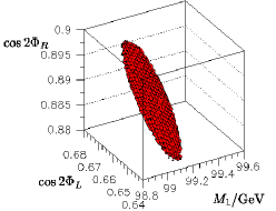
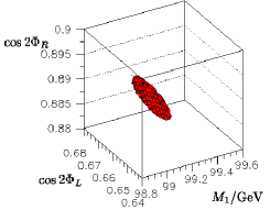
Figure 1: The $\Delta\chi^{2}=1$ contour in the {$M_{1},{\cos 2\Phi_{L}},\cos 2\Phi_{R}$} parameter space derived a) from the LC data and b) from the joint analysis of the LC data and LHC data [97].

In fig. 1a the contour of $\Delta\chi^{2}=1$ is shown in the $M_{1},{\cos 2\Phi_{L}},\cos 2\Phi_{R}$ parameter space along with its three 2dim projections. The projection of the contours onto the axes determines 1$\sigma$ errors for each parameter.

Values obtained for $M_{1},{\cos 2\Phi_{L}},\cos 2\Phi_{R}$ together with $m_{\tilde{\chi}^{\pm}_{1}}$ can be inverted to derive the fundamental parameters $M_{2}$, $\mu$ and $\tan\beta$. At the same time the masses of the heavy chargino and neutralinos are predicted, see table 3. As can be seen in table 3, the parameters $M_{1}$ and $M_{2}$ are determined at the level of a few per-mil. The $\mu$ is reconstructed within a few per-cent, while for $\tan\beta$ the error is of order 15%.

	SUSY Parameters				Mass Predictions
	$M_{1}$	$M_{2}$	$\mu$	$\tan\beta$	$m_{\tilde{\chi}^{\pm}_{2}}$	$m_{\tilde{\chi}^{0}_{3}}$	$m_{\tilde{\chi}^{0}_{4}}$
LC	$99.1\pm 0.2$	$192.7\pm 0.6$	$352.8\pm 8.9$	$10.3\pm 1.5$	$378.8\pm 7.8$	$359.2\pm 8.6$	$378.2\pm 8.1$
LC/LHC	$99.1\pm 0.1$	$192.7\pm 0.3$	$352.4\pm 2.1$	$10.2\pm 0.6$	$378.5\pm 2.0$	$358.8\pm 2.1$	–

Table 3: SUSY parameters with 1$\sigma$ errors derived from the analysis of the LC data and from the combined analysis of the LHC and LC data (with $\delta m_{\tilde{\chi}^{0}_{2}}=0.08$ GeV and $\delta m_{\tilde{\chi}^{0}_{4}}=2.23$ GeV derived from the LHC when using the LC input of $\delta m_{\tilde{\chi}^{0}_{1}}=0.05$ GeV) collected at the first phase of operation. Shown are also the mass predictions of the heavier chargino/neutralinos.

3.2 COMBINED STRATEGY FOR THE LHC AND LC

A rather large error of the $\mu$ parameter derived above stems from the gaugino-dominated character of the light charginos/neutralinos in the SPS1a scenario. A significant improvement for the $\mu$ (and $\tan\beta$) is expected with additional information on heavy neutralinos available from the LHC.

The LHC will provide a first measurement of the masses of ${\tilde{\chi}}^{0}_{1}$, ${\tilde{\chi}}^{0}_{2}$ and ${\tilde{\chi}}^{0}_{4}$, see. The measurements of ${\tilde{\chi}}^{0}_{2}$ and ${\tilde{\chi}}^{0}_{4}$ will be achieved through the study of the processes $\tilde{\chi}^{0}_{i}\rightarrow\tilde{\ell}\ell\rightarrow\ell\ell{\tilde{\chi}}^{0}_{1}$, (with $i=2,4$) in which the invariant mass of the two leptons in the final state shows an abrupt edge at $(m^{{\rm max}}_{l^{+}l^{-}})^{2}=m_{\tilde{\chi}^{0}_{i}}^{2}(1-m^{2}_{\tilde{\ell}}/m_{\tilde{\chi}^{0}_{i}})(1-m_{\tilde{\chi}^{0}_{1}}/m^{2}_{\tilde{\ell}})$.

With the LHC data, the achievable precision on $m_{{\tilde{\chi}}^{0}_{2}}$ and $m_{{\tilde{\chi}}^{0}_{4}}$ is expected be respectively 4.5 and 5.1 GeV for an integrated luminosity of 300 fb^-1. However, since the uncertainty on the $m_{\tilde{\chi}^{0}_{2}}$ and $m_{\tilde{\chi}^{0}_{4}}$ depends both on the endpoint determination and also on $m_{\tilde{\chi}^{0}_{1}}$ and $m_{\tilde{\ell}}$, a much higher precision can be achieved with $m_{\tilde{\chi}^{0}_{1}}$, $m_{\tilde{e}_{R}}$ and $m_{\tilde{e}_{L}}$ measured at the LC with precisions respectively of 0.05, 0.05 and 0.2 GeV, table 1. With this input the precisions on the LHC+LC measurements of $m_{\tilde{\chi}^{0}_{2}}$ and $m_{\tilde{\chi}^{0}_{4}}$ become: $\delta m_{\tilde{\chi}^{0}_{2}}=0.08$ GeV and $\delta m_{\tilde{\chi}^{0}_{4}}=2.23$ GeV. Performing again the $\Delta\chi^{2}$ test with this additional input one gets a significant improvement in the accuracy, see fig. 1b and table 3 for the final results. The accuracy for the parameters $\mu$ and particularly $\tan\beta$ is now much better, better than from other SUSY sectors [98, 99, 100] (and references therein).

4 SUMMARY

We have worked out in a specific example, an mSUGRA scenario with rather high $\tan\beta=10$, how the combination of the results from the two accelerators, LHC and LC, allows a precise determination of the fundamental SUSY parameters without assuming a specific supersymmetry breaking scheme. We have shown that a promising hand-in-hand procedure consists of feeding the LSP and slepton masses from the LC to the LHC analyses and injecting back a precise experimental determination of the ${\tilde{\chi}}^{0}_{2}$ and ${\tilde{\chi}}^{0}_{4}$ masses. It provides a determination of $M_{1}$, $M_{2}$, $\mu$ at the $\leq O(1\%)$ level and of (rather high) $\tan\beta$ of the order of $\leq$ 10%, reaching a stage where radiative corrections become relevant in the electroweak sector and which will have to be taken into account in future fits.

ACKNOWLEDGEMENTS

The authors would like to thank G. Weiglein for motivating this project. We thank the organisers for the wonderful atmosphere at the Les Houches workshop. We are indebted to G. Blair, U. Martyn and W. Porod for providing the errors for simulated mass measurements at the LC. The work is supported in part by the European Commission 5-th Framework Contract HPRN-CT-2000-00149. JK was supported by the KBN Grant 2 P03B 040 24 (2003-2005).

Part IX Proposal For A New Reconstruction Technique For Susy Processes At The LHC

M.M. Nojiri, G. Polesello and D.R. Tovey

1 INTRODUCTION

The potential of the LHC for SUSY parameter determination has been studied in great detail for the past seven years. One of the most promising methods involves the selection of events from a single decay chain near the kinematic endpoint. Information on the masses involved in the cascade decay can be extracted from the endpoint measurements. It has been established that one can achieve a few percent accuracy for sparticle mass reconstruction using this technique with sufficient statistics.

In this paper we propose a new method for reconstructing SUSY events which does not rely only on events near the endpoint. Instead one kinematically solves for the neutralino momenta and masses of heavier sparticles using measured jet and lepton momenta and a few mass inputs.

To illustrate the idea we take the following cascade decay chain

$$\tilde{g}\rightarrow\tilde{b}b\rightarrow\tilde{\chi}^{0}_{2}bb\rightarrow\tilde{\ell}bb\ell\rightarrow\tilde{\chi}^{0}_{1}bb\ell\ell.$$ (1)

This decay chain is approximately free from SM background with appropriate cuts. The five SUSY particles which are involved in the cascade decay have five mass shell conditions;

$$m^{2}_{\tilde{\chi}^{0}_{1}} = p^{2}_{\tilde{\chi}^{0}_{1}},$$ (2)

$$m^{2}_{\tilde{\ell}} = (p_{\tilde{\chi}^{0}_{1}}+p_{\ell_{1}})^{2},$$ (3)

$$m^{2}_{\tilde{\chi}^{0}_{2}} = (p_{\tilde{\chi}^{0}_{1}}+p_{\ell_{1}}+p_{\ell_{2}})^{2},$$ (4)

$$m^{2}_{\tilde{b}} = (p_{\tilde{\chi}^{0}_{1}}+p_{\ell_{1}}+p_{\ell_{2}}+p_{b_{1}})^{2},$$ (5)

$$m^{2}_{\tilde{g}} = (p_{\tilde{\chi}^{0}_{1}}+p_{\ell_{1}}+p_{\ell_{2}}+p_{b_{1}}+p_{b_{2}})^{2}.$$ (6)

Of these five masses, $m_{\tilde{\chi}^{0}_{1}}$,$m_{\tilde{\chi}^{0}_{2}}$ and $m_{\tilde{\ell}}$ can be measured at the LHC using first generation squark cascade decays with an accuracy of $\sim$ 10% (the mass difference is measured more precisely). Moreover, with input from a future high energy Linear Collider these masses might be determined with an accuracy $\sim O(1\%)$. We therefore assume for the present work that the masses of the two lighter neutralinos and of the right handed slepton are known, and we ignore the corresponding errors.

For a $bb\ell\ell$ event, the equations contain six unknowns ($m_{\tilde{g}}$, $m_{\tilde{b}}$ and $p_{\tilde{\chi}^{0}_{1}}$) which satisfy five equations. For two $bb\ell\ell$ events, we have ten equations while we only have ten unknowns (two neutralino four momenta, $m_{\tilde{g}}$ and $m_{\tilde{\chi}^{0}_{1}}$ ). Mathematically, one can obtain the sbottom and gluino masses and all neutralino momenta if there are more than two $bb\ell\ell$ events.

We call this technique the “mass relation method” as one uses the fact that sparticle masses are common for events which go though the same cascade decay chain. Note events need not be near the endpoint of the decay distribution to be relevant to the mass determination. In the next section we demonstrate the practical application of this method to measurement of the masses of the gluino and sbottom.

As a byproduct of the technique, once the mass of the squark and of all the sparticles involved in the decay are known, the momentum of the lighter neutralino can be fully reconstructed, and this further constrains the event.

In SUSY events sparticles are always pair produced and there are two lightest neutralinos in the event. If squark decays via $\tilde{q}\rightarrow\tilde{\chi}^{0}_{2}\rightarrow\tilde{\ell}\rightarrow\tilde{\chi}^{0}_{1}$ can be identified on one side of the event then the neutralino momentum can be reconstructed as described above. The transverse momentum of the lightest neutralino in the other cascade decay can then be obtained using the following equation

$${\bf p_{T}}(\tilde{\chi}^{0}_{1}(2))={\bf p_{T}}({\rm miss})+{\bf p_{T}}(\tilde{\chi}^{0}_{1}(1)),$$ (7)

provided that there are no hard neutrinos involved in the decay. This transverse momentum can be used to constrain the cascade decay of the other sparticle.

For the case where the other squark decays via $\tilde{q}\rightarrow\tilde{\chi}^{+}_{1}q\rightarrow\tilde{\chi}^{0}_{1}qW$ followed by $W\rightarrow q^{\prime}q^{\prime\prime}$, the chargino mass can be determined by using Eq. (7) and the following relations,

$$p_{\tilde{q}} = p_{\tilde{\chi}^{0}_{1}(2)}+p_{j}+p_{W},$$ (8)

$$p^{2}_{\tilde{q}} = m^{2}_{\tilde{q}},$$ (9)

where $p_{j}$ is the momentum of the selected high $p_{T}$ jet which comes from the squark decay and $p_{W}$ is the momentum of the two jet system consistent with the $W$ interpretation. The neutralino momentum resolution is important for the chargino mass reconstruction and we discuss this in section 3. The reconstruction will be discussed in a separate contribution[101].

The full reconstruction technique can be extended for higgs mass reconstruction. In section 4, we discuss the heavy higgs mass determination from the process $H\rightarrow\tilde{\chi}^{0}_{2}\tilde{\chi}^{0}_{2}$ followed by $\tilde{\chi}^{0}_{2}\rightarrow\tilde{\ell}\ell\rightarrow ll\tilde{\chi}^{0}_{1}$. This process is also useful for discovery of heavy higgs bosons. The four lepton momenta and missing momentum can be used to reconstruct the higgs mass assuming that the $p_{T}$ of the higgs boson is very small.

2 GLUINO CASCADE DECAY

We first discuss the results of a simulation study of the process where a gluino cascade decays into a sbottom at model point SPS1a[30]. The relevant sparticle masses for this study are listed in Table 1. The events were generated using the HERWIG 6.4 generator [12] [87] and passed through ATLFAST [88], a parametrised simulation of the ATLAS detector.

$m_{\tilde{g}}$	$m_{\tilde{b}_{1}(2)}$	$m_{\tilde{\chi}^{0}_{2}}$	$m_{\tilde{\ell}_{R}}$	$m_{\tilde{\chi}^{0}_{1}}$
595.2	491.9(524.6)	176.8	136.2	96.0

Table 1: Some sparticle masses in GeV at SPS1a.

We study only events which contain the cascade decay shown in Eq.(1). We then apply the following preselections to reduce backgrounds:

• $p_{T}^{miss}>100$ GeV

• $M_{\rm eff}>600$ GeV

• at least 3 jets with $p_{T1}>150$ GeV, $p_{T2}>100$ GeV and $p_{T3}>50$ GeV.

• exactly two jets with $p_{T}>50$ GeV tagged as $b$-jets

• exactly two OS-SF leptons with $p_{Tl1}>20$ GeV, $p_{Tl2}>10$ GeV, and invariant mass $40$GeV$<m_{ll}<78$ GeV.

The solution of Eq. (6) can be written in the following form:

$$m^{2}_{\tilde{g}} = F_{0}+F_{1}m^{2}_{\tilde{b}}\pm F_{2}D,$$ (10)

$${\rm where}\ \ D^{2} \equiv D_{0}+D_{1}m^{2}_{\tilde{b}}+D_{2}m^{4}_{\tilde{b}}.$$ (11)

Here $F_{i}$ and $D_{i}$ depend upon $p_{\ell_{i}}$ and $p_{b_{i}}$ and the neutralino and slepton masses. In the event, there are two $b$ jets and we assume that the $b$ jet with larger $p_{T}$ originates from the $\tilde{b}$ decay. The two leptons must come from $\tilde{\chi}^{0}_{2}$ and $\tilde{\ell}$ decay. There are maximally four sets of gluino and sbottom mass solutions together with two lepton assignments for each decay, because we cannot determine from which decay the lepton originates. To reduce combinatorics we take the event pair which satisfies the following conditions:

• Only one lepton assignment has a solution to the Eq. (11)

• For a pair of events there are only two solutions and there is a difference of more than 100 GeV between the two gluino mass solutions.

Figure 1: $m_{\tilde{g}}$ obtained by using Eq. (11) for two $bb\ell\ell$ events.

In Fig 1, we plot the minimum $m_{\tilde{g}}$ solution which satisfies the conditions given above. The peak position is consistent with the gluino mass, and the error on the peak position obtained by a Gaussian fit is around 1.7 GeV for 100 fb^-1. For the events used in the reconstruction, each event is used on average five times. Note that the $\sigma$ of the Gaussian fit is large ($\sim 56.7$ GeV) and is determined by the resolution on the momentum measurement of the four $b$-jets. It is worth stressing that the results presented here were produced by using a parametrised simulation of the response of the ATLAS detector to jets, based on the results of a detailed simulation. Results which crucially depend on the detailed features of the detector response, such as the possibility of discriminating the two sbottom squarks (see below) need to be validated by an explicit detailed simulation of the detector performed on the physics channel of interest. We only attempt here to evaluate the impact of the new technique on sparticle reconstruction.

Once the gluino mass has been determined one can reconstruct the sbottom mass by fixing the gluino mass to the measured value. Here one need only solve Eq.(11), which involves only two $b$-jets in the fit, and therefore errors due to the jet resolution are expected to be less than those for the gluino mass reconstruction.

For each event, there are two sbottom mass solutions $m_{\tilde{b}}$(sol1) and $m_{\tilde{b}}$(sol2), each sensitive to the gluino mass input. The difference between the gluino and sbottom mass solutions is however stable against variation in the assumed gluino mass. The mass itself may have a large error in the absolute scale, but the mass differences are obtained rather precisely, as is the case in the endpoint method.

In Fig. 2 (left), we plot the solutions for all possible lepton combinations in the $m_{\tilde{g}}-m_{\tilde{b}}$ (sol1) $m_{\tilde{g}}-m_{\tilde{b}}$ (sol2) plane. Here we use the $b$-parton momentum obtained from generator information. One of the solutions tends to be consistent with the input sbottom mass. Moreover the two decay modes $\tilde{g}\rightarrow\tilde{b}_{1}b$ and $\tilde{b}_{2}b$ are clearly separated.

We can compare the results from the previous analysis with those from the endpoint analysis[85], where one uses approximate the formula

$${\bf p}_{\tilde{\chi}^{0}_{2}}=\left(1-\frac{m_{\tilde{\chi}^{0}_{1}}}{m_{\ell\ell}}\right){\bf p}_{\ell\ell}.$$ (12)

This formula is correct only at the endpoint of the three body decay $\tilde{\chi}^{0}_{2}\rightarrow\chi^{0}_{1}\ell\ell$, but is nevertheless approximately correct near the edge of $\tilde{\chi}^{0}_{2}\rightarrow\tilde{\ell}\ell\rightarrow\ell\ell\tilde{\chi}^{0}_{1}$ for SPS1a. The sbottom mass obtained by using Eq.(12) is shown in Fig. 2(right). For this case, the $\tilde{b}_{2}$ peak at 70.6 GeV is not separated from the $\tilde{b}_{1}$ peak at 103 GeV.

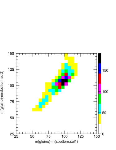
Figure 2: The distribution of $m_{\tilde{g}}-m_{\tilde{b}}$ calculated using the parton level $b$ momentum by solving Eq.(6) (left) and using the approximate relation Eq. 12(right).

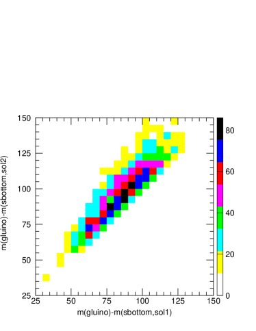
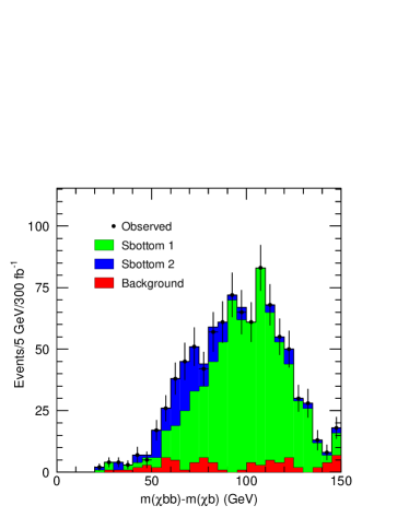
Figure 3: As for Fig. 2 but with the $b$ jet momentum used instead of the $b$ parton momentum.

The $\tilde{b}_{1}$ mass, or the weighted average of the sbottom masses, is easily obtained. The $b$ jet resolution is not sufficient however to clearly separate the $\tilde{b}_{1}$ and $\tilde{b}_{2}$. This can be seen in Fig. 3 where the plots show the distributions corresponding to Fig.2(left) and (right) but now with the $b$ parton momenta replaced by $b$ jet momenta. For the endpoint analysis (Fig.3 right), a correct evaluation of the sbottom masses would require a fit taking into account the shape of the response of ATLAS to b-jets. In order to approximately evaluate the achievable statistical precision, a naive double gaussian fit was performed on the distribution shown in Fig.3 right, which corresponds to $\int dtL=300$ fb^-1. The resulting statistical uncertainties are $\pm 1$ GeV ($\pm 2.5$ GeV) for the $m_{\tilde{g}}-m_{\tilde{b}_{1}}$($m_{\tilde{g}}-m_{\tilde{b}_{2}}$ ) peak positions respectively. Additional systematic uncertainties, not yet evaluated, as well a 1% error due to the uncertainty on the jet energy scale should also be considered. These numbers are obtained assuming the presence of two gaussian peaks in the data.

For the mass relation method the number of events available for the study is larger by a factor of 2 because events away from the endpoints can be used. We also use the exact formula for the mass relation method. Although the analysis is more complicated due to the multiple solutions, we believe it to be a worthwhile technique for use when attempting to reconstruct the $\tilde{b}_{1}$ and $\tilde{b_{2}}$ masses.

3 NEUTRALINO MOMENTUM RECONSTRUCTION

In this section, we discuss the reconstruction of the momentum of the lightest neutralino. As we have discussed already, the mass shell condition can be solved for long decay cascades, such as $\tilde{q}\rightarrow\tilde{\chi}^{0}_{2}q\rightarrow\tilde{\ell}q\ell\rightarrow\tilde{\chi}^{0}_{1}q\ell\ell$. For this process we have two neutralino momentum solutions for each lepton assignment. One may wonder if the solutions for the neutralino momentum might be smeared significantly, because of the worse jet energy resolution as compared to leptons, and the jet $p_{T}$ is generally much larger than the neutralino momentum for the cascade decay. In Fig. 4(left) we show the distribution of $p_{T}$(reco)/$p_{T}$(truth) for the point studied in [101]. Here we choose the correct lepton combination using generator information, and take the solution which minimizes $|p_{T}$(reco)/$p_{T}$(truth)$-1|$. Except for the case where we took the wrong jet as input the reconstructed $p_{T}$ is within 20% of the true neutralino momentum. The result for the gluino cascade decay into sbottom Eq.(1) is similar.

In Fig. 4(right) we show a similar reconstruction for the gluino cascade decay, but unlike Fig.4(left), we use both lepton combinations. We fix the gluino mass to the input value and take events where one of the four sbottom mass solutions is consistent with the input sbottom mass such that $|m_{\tilde{b}_{1}}-m_{\tilde{b}}({\rm best})|<10$ GeV. We then take the solution where the sbottom mass is closest to the input $m_{\tilde{b}_{1}}$. There are still two $p_{\tilde{\chi}^{0}_{1}}$ solutions, and we choose the one which minimize $|{\rm min}(p_{T}({\rm reco})/p_{T}({\rm truth}),p_{T}({\rm truth})/p_{T}({\rm reco}))-1|$. The neutralino momentum resolution is worse than that obtained using the correct lepton assignments only. Nevertheless a significant fraction of events are reconstructed with $0.8<|{\bf p}({\rm reco})/{\bf p}({\rm truth})|<1.2$.

Figure 4: Left: The calculated $\tilde{\chi}^{0}_{1}$ transverse momentum divided by the true transverse momentum. The decay $\tilde{q}_{L}\rightarrow\tilde{\chi}^{0}_{2}q\rightarrow\tilde{\ell}q\ell\rightarrow\tilde{\chi}^{0}_{1}q\ell\ell$ is studied for the model point used for the chargino study: $m_{0}=100$ GeV, $m_{1/2}=300$ GeV, $A_{0}=-300$ GeV, $\tan\beta=6$, and $\mu>0$. Only the correct lepton choice is used. Right: $|{\bf p}$(reco)$/{\bf p}$(truth)$|$ for the decay chain Eq.(1) for SPS1a.

4 HIGGS MASS RECONSTRUCTION

A promising decay for the observation of heavy and pseudo-scalar higgs bosons in the difficult region with intermediate $\tan\beta$ is the decay into two neutralinos. When both neutralinos decay through the chain

$$\tilde{\chi}^{0}_{2}\rightarrow\tilde{\ell}_{R}\ell\rightarrow\ell\ell\tilde{\chi}^{0}_{1}$$

the resulting signature consists of events with four isolated leptons (paired in opposite-sign same-flavour pairs) and no jet activity. The main SM backgrounds to this signature are $t\bar{t}$ production, where both the $b$-jets and the $W$s decay into leptons and $Zbb$ production. The key element for the rejection of these backgrounds is the fact that the leptons from $b$ decays are not isolated. A detailed study of the performance of lepton isolation in the detector is needed to assess the visibility of the signal. Additionally there is an important SUSY background, including irreducible backgrounds from direct slepton and gaugino decay. Full background studies as a function of the SUSY parameters were performed by the ATLAS and CMS Collaborations [79, 102]. We propose here, along the lines of the previous sections, a technique for the complete reconstruction of the higgs peak, based on the knowledge of the masses of $\tilde{\chi}_{2}^{0}$, $\tilde{\ell}_{R}$ and $\tilde{\chi}_{1}^{0}$. In this case one has 8 unknown quantities: the 4-momenta of the two LSP’s, and 8 constraints: six on-shell mass constraints (3 for each leg), and the two $E_{T}^{miss}$ components.

To demonstrate the power of the method, we apply it to Point SPS1a, for which the mass of the $A$ and of the $H$ is $\sim 394$ GeV. The BR into $\tilde{\chi}^{0}_{2}\tilde{\chi}^{0}_{2}$ is 6% (1%) for the $A$($H$). We perform the study on 1000 events for

$$A\rightarrow\tilde{\chi}^{0}_{2}\tilde{\chi}^{0}_{2}\rightarrow\ell\ell\ell\ell\tilde{\chi}^{0}_{1}\tilde{\chi}^{0}_{1}$$

corresponding approximately to the expected statistics for 300 fb^-1. We simply require 2 isolated leptons with $p_{T}>20$ GeV and 2 further isolated leptons with $p_{T}>10$ GeV, all within $|\eta|<2.5$. The efficiency of these cuts is $\sim 60\%$.

We have not performed any background simulations because at this stage we only wish to explore the viability of the full reconstruction technique. The main problem for the reconstruction is the correct assignment of the leptons to the appropriate decay chain. The first selection is based on requiring a unique identification of the lepton pairs coming from the decays of the two $\tilde{\chi}^{0}_{2}$s. We therefore require that either of the following two criteria is satisfied:

• the flavour configuration of the leptons is $e^{+}e^{+}\mu^{+}\mu^{-}$

• the lepton configuration is either $e^{+}e^{-}e^{+}e^{-}$ or $\mu^{+}\mu^{-}\mu^{+}\mu^{-}$, but for one of the two possible pairings the invariant mass of one of the pairs is larger than 78 GeV, i.e. above the lepton-lepton edge for the $\tilde{\chi}^{0}_{2}$ decay.

The total efficiency after these cuts is $\sim 30\%$. At this point, on each of the two legs there is still an ambiguity due to the fact that each lepton can be either the product of the first or of the second step in the decay chain. This gives 4 possible combinations. Furthermore, the full reconstruction results in a quartic equation which can have zero, two or four solutions. We show in Fig. (5) the distribution of the calculated $A$ mass for all of the retained combinations as a full line. The dashed line shows the combinations with the wrong lepton assignment. A clear and narrow peak emerges over the combinatorial background. The width is approximately 6 GeV, determined by the resolution of the measurement of the momentum of the leptons.

Figure 5: Reconstructed mass of the $A$.

5 CONCLUSIONS

In this contribution, we have described a novel technique for reconstructing the mass and momenta of SUSY particles. This technique does not rely on any approximate formulae nor on endpoint measurements. All events contribute to the sparticle mass determination and decay kinematics reconstruction, even if they are away from the endpoint of the distribution. The method may be particularly useful when the SUSY mass scale is large. In that case the statistics can be so low that the endpoint cannot be seen clearly while the SUSY sample itself is very clean.

The method applies most effectively when we know some of the sparticles’ masses exactly, because the number of unknown parameters in e.g. Eq.(6) is reduced. In the particular case where some of the sparticle masses are measured at a LC the sparticle cascades may be solved completely and study of the decay distributions and higher mass determination becomes possible at LHC.

When all the sparticle masses are known the neutralino momentum can be reconstructed if four sparticles are involved in the cascade decay. The sparticles would be pair produced, and if we can identify both of the cascade decay chains in the events then we only need six sparticles in the cascade decay to solve both of the neutralino momenta on account of the missing momentum constraint. The reconstruction of sparticle momenta provides us with an interesting possibility for studying the decay distribution at the LHC.

On the other hand, our method is not valid when some of the particles in the cascade produce hard neutrinos. This is unfortunately the case when the chargino decays into (s)leptons, when a $\tilde{\tau}$ is involved in the decay, or when a $W$ is produced and decays leptonically. If such SUSY decay processes dominate then this method may not be useful.

Acknowledgments

This work was performed in the framework of the workshop: Les Houches 2003: Physics at TeV Scale Colliders. We wish to thank the staff and organisers for all their hard work before, during and after the workshop. We thank members of the ATLAS Collaboration for helpful discussions. We have made use of ATLAS physics analysis and simulation tools which are the result of collaboration-wide efforts. DRT wishes to acknowledge PPARC and the University of Sheffield for support.

Part X Building on a Proposal for a New Reconstruction Technique for SUSY Processes at the LHC

C.G. Lester

1 INTRODUCTION

The authors of [103] propose “a new reconstruction technique for SUSY processes at the LHC”. Their method is described in detail in their article elsewhere in these proceedings, and so only an outline of their method will be provided here. The reader is strongly encouraged to read their article before reading this one.

The authors of [103] refer to their technique as the “mass relation method”. I wish to narrow the meaning of this phrase, as I want to draw a distinction between (1) the idea that makes the whole method work, and (2) any particular implementation of that idea. I will use the phrase “mass relation method” to describe any method which, for its success, is forced to rely on the extraction of information from two or more independent events which are related only by their sharing similar or identical particle content.

2 OUTLINE OF ORIGINAL IMPLEMENTATION

In [103] it is suggested that “when several sparticle masses are known, the kinematics of SUSY decay processes observed at the LHC can be solved if the cascade decay contains sufficient steps”. Therein, an original implementation is described which accomplishes this solution. The efficacy of this implementation is demonstrated using the decay chain

$${\tilde{g}}\rightarrow{\tilde{b}}b\rightarrow{{\tilde{\chi}}^{0}_{2}}bb\rightarrow{\tilde{l}}bbl\rightarrow{{\tilde{\chi}}^{0}_{1}}bbll.$$ (1)

In order to complete the demonstration, the authors make the assumption that “… the masses of the two lighter neutralinos and the right handed slepton are known, and [they] ignore the corresponding errors”. By ignoring the corresponding errors, they in effect demonstrate their method in a scenario in which the slepton and neutralino masses are already known to something like the one-percent level – something not usually assumed to be possible with LHC data alone. Having made these assumptions, the authors set out to measure the masses of the two remaining sparticles. Firstly, on an event-pair by event-pair basis, they obtain an estimate of their gluino mass with an accuracy of about $\pm 60\leavevmode\nobreak\ {{\mathrm{GeV}}}$ (approximately 10%). By histogramming the results from all these event-pairs an overall measurement of the gluino mass is obtained with an error of a few $GeV$. This measurement is then fed back into the events which are analysed in a second pass in order to make a measurement of the sbottom mass.

2.1 A small part of the original implementation in more detail

As already mentioned in Section 1, the authors begin by assuming prior knowledge of $m_{{\tilde{\chi}}^{0}_{1}}$, $m_{\tilde{l}}$ and $m_{{\tilde{\chi}}^{0}_{2}}$; that is to say the masses of the two lightest neutralinos and the mass of the slepton participating in the decay chain shown in Equation (1). This leaves in any one event the six unknown real quantities comprising: $m_{\tilde{g}}$, $m_{\tilde{b}}$ and the four components of $p_{{\tilde{\chi}}^{0}_{1}}$. These six unknowns, are however constrained to satisfy the five mass constraints:

$$m_{{\tilde{\chi}}^{0}_{1}}^{2} = p_{{\tilde{\chi}}^{0}_{1}}^{2},$$

$$m_{\tilde{l}}^{2} = (p_{{\tilde{\chi}}^{0}_{1}}+p_{l_{1}})^{2},$$

$$m_{{\tilde{\chi}}^{0}_{2}}^{2} = (p_{{\tilde{\chi}}^{0}_{1}}+p_{l_{1}}+p_{l_{2}})^{2},$$ (2)

$$m_{\tilde{b}}^{2} = (p_{{\tilde{\chi}}^{0}_{1}}+p_{l_{1}}+p_{l_{2}}+p_{b_{1}})^{2},\mbox{\qquad and}$$

$$m_{\tilde{g}}^{2} = (p_{{\tilde{\chi}}^{0}_{1}}+p_{l_{1}}+p_{l_{2}}+p_{b_{1}}+p_{b_{2}})^{2},$$

in which $p_{l_{1}}$, $p_{l_{2}}$, $p_{b_{1}}$ and $p_{b_{2}}$ are the four-momenta of the emitted standard model particles. Since the number of unknowns (six) exceeds the number of constraints (five) it is not possible to conclude much from one event.

Taking a second event together, however, the number of unknowns rises by only four, namely the four components of the ${{\tilde{\chi}}^{0}_{1}}$-momentum in the new event. As ever, the new event, like the old, will satisfy another five mass constraints of the form shown in Equation (2). With two events, then, the number of unknowns and number of constraints have each risen to ten. So in principle, with only two non-degenerate events, it is now possible to determine all the unknowns. This amounts to full reconstruction of both events and determination of $m_{\tilde{g}}$ and $m_{\tilde{b}}$. The interested reader is directed to [103] to see how the authors handle choice-ambiguities that arise from (a) the solution of simultaneous quartic and quadratic equations, and (b) lack of knowledge of which of the two observed leptons is $l_{1}$ and which of the two observed $b$-tagged jets came from $b_{1}$.

The implementation of [103] proposes that one should do exactly as described above: namely consider events in pairs.

3 MOTIVATIONS FOR BUILDING ON THE ABOVE

A natural reaction on seeing the original implementation is to ask:

Since two events are better than one, why not consider even more?

The majority of the rest of this note tries to address the above question. The motivation for building on the above is that every new event adds five more constraints but only four more unknowns. Put another way, for every additional event that is acquired, one can either answer one new question, or else better constrain any answers that one already has. This note concentrates on the last of these two possibilities.

4 PROPOSAL FOR A “NEW IMPLEMENTATION” OF A MASS RELATION METHOD

4.1 General comments

The new proposal is to do nothing more than consider all the relevant events simultaneously.

In this note, we will not address the important question of whether, in a real LHC experiment, it would be possible to satisfy the preconditions for the success of any mass relation method, namely the requirements that it be possible to construct sufficiently pure samples of the appropriate standard model samples from chains of sufficiently similar or identical particle content. This needs to be addressed in further papers, and has already been considered in part by [103]. The intention of this note is only to look at what may be achieved if such selection were possible.

4.2 Detailed description of proposal

Ideally we would like to know the masses of the sparticles in our events. Realistically, we can only expect to find the masses within some finite precision or error. Bearing correlations in mind, the best we can expect to determine is the relative probability of any particular combination of the five masses ${\bf m}=(m_{{\tilde{\chi}}^{0}_{1}},m_{\tilde{l}},m_{{\tilde{\chi}}^{0}_{2}},m_{\tilde{b}},m_{\tilde{g}})$ given the data. In short, we would like to plot $p({\bf m}|{\mbox{data}})$.

By Bayes’ theorem, $p({\bf m}|{\mbox{data}})\propto p({\mbox{data}}|{\bf m})p_{0}({\bf m})$. The first factor, the likelihood, will be determined purely from the events considered and the mass relation method itself and is thus the objective “result” of this experiment. The last factor, the prior, incorporates all existing knowledge gained from other experiments (if you should wish to include them) and any subjective preferences you might have. Because we choose here to use a non-informative prior (uniform in the hierarchical sparticle masses) the reader may view the results at his or her discretion as either (a) simple plots of the objective likelihood distribution $p({\mbox{data}}|{\bf m})$, or else, (b) indicative of the results which a single experiment would provide $p({\bf m}|{\mbox{data}})$ in the absence of data from other experiments.

The only thing remaining to be defined is $p({\mbox{data}}|{\bf m})$. As the data consists of many independent events, we have $p({\mbox{data}}|{\bf m})=p({\mbox{event}_{1}}|{\bf m}).p({\mbox{event}_{2}}|{\bf m}).\cdot\cdot\cdot.p({\mbox{event}_{n}}|{\bf m}),$ and we are left needing to evaluate $p({\mbox{event}_{i}}|{\bf m})$ for a given event $i$.

Evaluating the event-likelihood $p({\mbox{event}_{i}}|{\bf m})$ properly and efficiently is the hard part. In principle there is only one right answer, which you would obtain by taking the square of the matrix element for the observed final state and integrating it over all the unknowns in the problem, namely the measurement errors and the momentum distribution of the unobserved chain progenitor. The answer you obtain will thus depend on which model assumptions you wish to make, e.g. whether you would choose to model the differing spins of the sparticles.

In order to meet the time constraints imposed by the submission of this note, however, it was necessary to implement the event-likelihood using an ad-hoc approximation. It is hoped that the approximation to the event-likelihood described later is sufficiently similar to the full form of $p({\mbox{event}_{i}}|{\bf m})$ that the basic features of the proposed technique can be demonstrated.

We construct the approximation to the event-likelihood used in this note as follows. For a given chain momentum hypotheses $H$ consistent with the given mass hypothesis ${\bf m}$, we can define a “distance” $\delta(H)$ between the observed and the true momenta of the visible particles produced in that chain by

$$\delta(H)=\epsilon_{l_{1}^{H}}^{2}/\sigma_{l}^{2}+\epsilon_{l_{2}^{H}}^{2}/\sigma_{l}^{2}+\epsilon_{b_{1}^{H}}^{2}/\sigma_{b}^{2}+\epsilon_{b_{2}^{H}}^{2}/\sigma_{b}^{2}$$ (3)

where (for example) $\epsilon_{l_{1}^{H}}^{2}/\sigma_{l}^{2}$ is square of the number of standard deviations by which the measured momentum of $l_{1}$ differs from a hypothesised true value $p^{H}_{l_{1}}$.

We can then perform a least-squares minimisation of $\delta(H)$ over all possible chain momentum hypotheses $H$ consistent with the given mass hypothesis ${\bf m}$. We now make the assumption that this least-squared minimisation will have provided us with the momenta which are most consistent with the observation and the mass hypothesis ${\bf m}$. Finally, then, we can approximate the event-likelihood by the simple process of evaluating the probability for the observed momenta to deviate as far as their observed values, assuming that the “true” momenta are given by the result of the fit. This approximation thus depends crucially on a good understanding of the measurement errors associated with the observed standard model particles.

The key features of this approximation to the event-likelihood are that it will be large when $p({\mbox{event}_{i}}|{\bf m})$ is large and small when $p({\mbox{event}_{i}}|{\bf m})$ is small. This gives us confidence that the maxima and minima of the event-likelihood will be well approximated. It will most probably not be the case, however, that the widths of the resulting distributions or the finer shape details (for a particular number of events) can be completely relied upon. This, though undesirable, is not too great a problem as the widths naturally scale with the number of events analysed. For this reason, the approximation may be thought of as resulting in an uncertainty in how many events are necessary to achieve a given reconstruction error, rather than an uncertainty in the quality of the reconstruction itself.

5 RESULTS OF NEW PROPOSAL

In order to demonstrate the potential of the above technique, it is necessary to generate some events for analysis. A toy montecarlo was used to generate these events only. For the reasons of Section 4.1 it simulated only relativistic kinematics and decays were according to phase space only. In effect all particles were treated as scalars. Furthermore, only the chain described in Equation (1) was simulated. No extraneous particles were produced, and nor is there an “other side of the event”.

Events were simulated events using the following arbitrary values for the sparticle masses: $m_{{\tilde{\chi}}^{0}_{1}}=150\leavevmode\nobreak\ {{\mathrm{GeV}}}$, $m_{\tilde{l}}=200\leavevmode\nobreak\ {{\mathrm{GeV}}}$, $m_{{\tilde{\chi}}^{0}_{2}}=300\leavevmode\nobreak\ {{\mathrm{GeV}}}$, $m_{\tilde{b}}=500\leavevmode\nobreak\ {{\mathrm{GeV}}}$ and $m_{\tilde{g}}=650\leavevmode\nobreak\ {{\mathrm{GeV}}}$.

Measurement errors were simulated by randomised rescaling of the four momenta of the observed particles in a manner similar to that described in [104], but without $\eta$ and $\phi$ dependence in the resolutions. Lepton momenta were smeared by 1% and jet momenta by 5%. The reconstruction part of the analysis was handed the two lepton momenta in a random order and the two $b$-jet momenta in a random order so that it could not know which of them was which.

After generating 100 events of the form described above, the results shown in Figures 1 were obtained. Here we choose to plot $p({\bf m}|{\mbox{data}})$ by sampling from it using a Metropolis Markov-chain sampler [105], although this particular choice is unimportant.

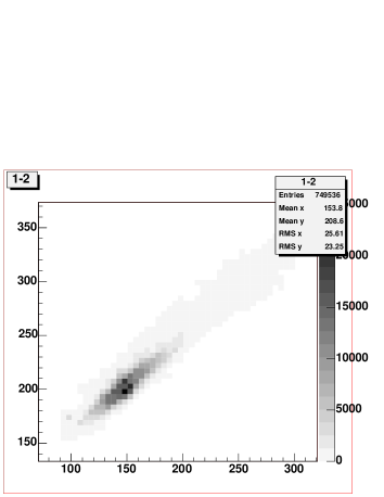
(a) $m_{\tilde{l}}$ against $m_{{\tilde{\chi}}^{0}_{1}}$

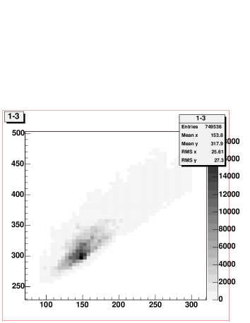
(b) $m_{{\tilde{\chi}}^{0}_{2}}$ against $m_{{\tilde{\chi}}^{0}_{1}}$

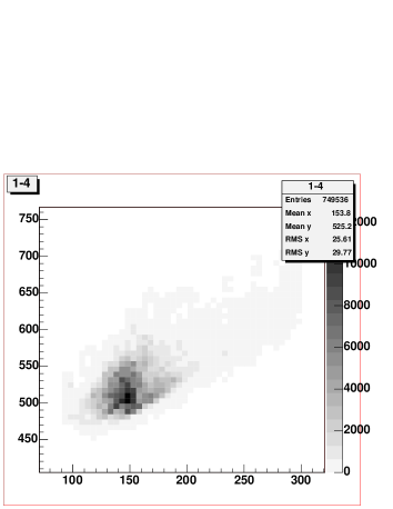
(c) $m_{\tilde{b}}$ against $m_{{\tilde{\chi}}^{0}_{1}}$

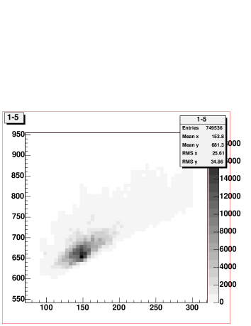
(d) $m_{\tilde{g}}$ against $m_{{\tilde{\chi}}^{0}_{1}}$

Figure 1: Samples drawn from $p({\bf m}|{\mbox{data}})$. Axes in ${{\mathrm{GeV}}}$.

Figure 1 shows how the reconstructed mass distributions of the heavier sparticles correlate with the reconstructed mass distribution of the lightest neutralino. The correlation show that at this point the mass differences tend to be measured more accurately than the absolute masses. The mass of the lightest neutralino is well reconstructed (input value $150\leavevmode\nobreak\ {{\mathrm{GeV}}}$) with an error of order approximately 17%. The reconstructed mass distributions of the remaining sparticles are similar to that of the lightest neutralino as the mass differences are constrained better than the masses themselves.

6 CONCLUSIONS

This note aims to convey the message that should it be possible at the LHC to isolate clean samples of the decay products of a hundred or so sparticle decay chains containing enough sufficiently similar or identical particles, then by using a mass relation method of the type proposed, one should be able to reconstruct the masses of all the sparticles in these decay chains to precisions of at least some tens of percent, depending on the number of these events.

Further work is needed to establish that the necessary sample purity is achievable, and to ascertain the effect that a better model for the event-likelihood would have on the widths of the reconstructed distributions. If the identified collections of outgoing particles are sufficiently pure and large, it does not seem unreasonable to believe that one might expect a precision on the reconstructed masses which is competitive with any other independent method found so far.

It seems likely that the usefulness of this method will be limited by the ability to produce the necessary pure samples of decay-chain products.

7 ACKNOWLEDGEMENTS

I would like to thank Mihoko Nojiri, Giacomo Polesello, Dan Tovey and Andy Parker for helpful discussions. I would also like to thank Ben Allanach for his own helpful comments and for encouragement. Finally I would like to thank Alan Barr for his own nit-picks and for drawing reference [103] to my attention.

Part XI Study of non-pointing photons at the CERN LHC

K. Kawagoe, M.M. Nojiri, G. Polesello and D. Prieur

1 GAUGE MEDIATION MODELS AND NON-POINTING PHOTONS

Origin of the SUSY breaking in the hidden sector and its mediation to the MSSM sector are key features of SUSY models. When hidden sector SUSY breaking is expressed by the order parameter $F$ and the scale of the mediation to the MSSM sector by $M$, the mass scale of MSSM sparticles $M_{SUSY}$ is of the order of $\lambda F/M$, where $\lambda$ is the coupling of the hidden sector to the MSSM sector. The SUSY breaking mediation may be due to renormalizable interactions, such as the gauge interaction. This is called “gauge mediation” (GM) models. In the GM models $M$ and $F$ are arbitrary and we expect $M\ll M_{\rm pl}$.

When $M\ll M_{\rm pl}$, the lightest SUSY particle (LSP) is the gravitino ($\tilde{G}$) in the GM models. The next lightest SUSY particle (NLSP) is a particle in the MSSM sector which decays into a gravitino. If the lightest neutralino ($\tilde{\chi}^{0}_{1}$) is the NLSP, the dominant decay mode is $\tilde{\chi}^{0}_{1}\rightarrow\gamma\tilde{G}$. The neutralino lifetime $c\tau$ is a function of $F_{0}$ and $m_{\tilde{\chi}^{0}_{1}}$, and the neutralino may be long-lived. Therefore it is an important subject to study non-pointing photons at the CERN LHC.

In a paper [106], a procedure is proposed to solve the gravitino momentum and $\tilde{\chi}^{0}_{1}$ decay position for the cascade decay $\tilde{\ell}\rightarrow\tilde{\chi}^{0}_{1}\ell\rightarrow\tilde{G}\ell\gamma$ using the ATLAS detector at the LHC. It is shown that one can determine the mass and lifetime of $\tilde{\chi}^{0}_{1}$. To this purpose, one need to measure the photon momentum and arrival time very precisely. A toy simulation is made under the following assumptions to the photon momentum resolution;

• A good angular resolution of $\sigma_{\theta}=60\ {\rm mrad}/\sqrt{E}$ is assumed, where $\theta$ is the polar angle of the photon momentum with respect to the beam axis and $E$ is the photon energy measured in GeV. This resolution is based on a simulation for pointing photons.

• The azimuthal angle of the photon momentum $\phi$ is only poorly measured by the electromagnetic (EM) calorimeter. The $\phi$ resolution is good only for the photons converted in the transition radiation tracker (TRT) located in the EM calorimeter.

The analysis takes two steps. First, events with converted non-pointing photons are selected. As the photon momentum is precisely measured, the events can be used to determine the mass of $\tilde{\chi}^{0}_{1}$. In solving the kinematics, the direction of the gravitino momentum is sensitive to the photon momentum. The mass resolution at GM point  G1 with $c\tau_{\tilde{\chi}^{0}_{1}}=100$cm is $\Delta m_{\tilde{\chi}^{0}_{1}}=3.5$ GeV for $10^{5}$ generated SUSY events, which corresponds to an integrated luminosity of 13.9 fb^-1.

Once the mass is determined precisely, the good $\phi$ resolution of the photon momentum is not required to solve the decay kinematics. The decay kinematics can be solved for all $\ell\gamma$ events with non-pointing photons, from the $\theta$ component of the photon momentum, the arrival time and position at the ECAL, and the lepton momentum. Therefore, all $\ell\gamma$ events with or without photon conversion can be used to determine the lifetime. The lifetime resolution for the GM point G1 is $\Delta c\tau/c\tau=0.045$ for the $10^{5}$ generated SUSY events.

Although the result looks nice, some of the assumptions in the paper may be too optimistic, and should be studied more realistically. Among them, the $\theta$ resolution obtained for pointing photons are used to estimate that for non-pointing photons. In this article we study the $\theta$ resolution for non-pointing photons by a full simulation and discuss the impacts to the GM study.

2 PARAMETRISATION OF ANGULAR RESOLUTION OF ATLAS BARREL ELECTROMAGNETIC CALORIMETER

In this part we try to obtain a more refined parametrization of the angular resolution for non-pointing photons with the ATLAS EM calorimeter. So far the resolution has been studied only for nearly pointing photons, i.e. photons coming from the ATLAS interaction point, and it is of the order of 60 ${\rm mrad}/\sqrt{E}$ [107, 79]. In the following we will try to see which resolution is achievable for non-pointing photons using a full simulation of the ATLAS detector.

The EM calorimeter [79] is a projective calorimeter with a good granularity to perform precision measurements of the shower position. It is longitudinally divided into three compartments: strip, middle and back compartment. The strip section is segmented along $\eta$ into very thin cells of $\Delta\eta=0.003125$, leading to a resolution on $\eta$ position with pointing photons of $0.30\times 10^{-3}$. The middle compartment has a wider $\eta$ granularity of $\Delta\eta=0.025$ and it is designed to contain most of the shower energy. It has a resolution on $\eta$ position of $0.83\times 10^{-3}$. By combining the measurement of the $\eta$ position in the first two compartments, it is possible to determine the shower direction in $\eta$.

For this study, different samples of single photons have been generated. Each of these samples consist of $20000$ photons of $p_{t}=60$ GeV, randomly triggered with $\eta$ from $-1.4$ to $1.4$. Pointing photons were generated at ATLAS origin with a spread on the position of the generation vertex of $5.6$ cm along Z axis and $15$ $\mu$m along radial axis, as it should be in ATLAS final setup. For non-pointing photon samples, the generation vertex has been shifted along ATLAS Z axis with values from $10$ cm to $150$ cm. No spread on the generation vertex position has been applied for these dataset. Finally all of these events were fully simulated using Dice/Atlsim (v3.2.1), the Geant3 ATLAS detector description [108].

Here we focus only on the barrel part of the EM calorimeter. The reconstruction of all events has been done using ATLAS standard reconstruction software (Athena v6.5.0). No electronic noise or pile-up have been added in the reconstruction. The noise will certainly contribute to degrade the resolution, however this has not been studied yet.

With the $\eta$ position, in each layer of the calorimeter ($\eta_{1}$,$\eta_{2}$) and using a parametrization of the shower depth for each layers ($R_{1}(\eta_{1})$,$R_{2}(\eta_{2})$) [107], we are able to reconstruct the shower axis $\eta_{pointing}$ using the following relation:

$$\sinh(\eta_{pointing})=\frac{R_{2}(\eta_{2})\sinh(\eta_{2})-R_{1}(\eta_{1})\sinh(\eta_{1})}{R_{2}(\eta_{2})-R_{1}(\eta_{1})}$$ (1)

The standard reconstruction uses a sliding window algorithm to find regions of interest in the calorimeter, then $3\times 3$ ($\eta\times\phi$) clusters are made in order to compute the $\eta$ barycenter of the shower in each layer. This position is the average of cells $\eta$ position weighted by energy in each cell:

$$\overline{\eta}=\frac{\sum{\eta_{i}E_{i}}}{\sum E_{i}}$$ (2)

The angular resolution achieved using the standard reconstruction is shown in Fig. 1 as a function of the position of the generation along ATLAS Z axis. The resolution is significantly degraded from 60 mrad for $Z_{vertex}=0$ cm to about 800 mrad for $Z_{vertex}=100$ cm. This is due to several effects. First, the S-shape corrections, that were tuned for pointing photons, are no longer valid and tend to degrade the resolution for large deviation from pointing. The S-shape effect is a distortion of the reconstructed $\eta$ position due to the finite cluster size. Then the $3\times 3$ clusters are no longer sufficient to contain all the shower and some energy leakage outside the cluster is possible. Another point is that Eq. (2) is no more true for non-pointing photons and gives rise to a systematic shift in computing $\eta$ position for each layer. Finally, the shower depth parametrization, tuned from pointing photons, is also no more valid for large deviation from pointing.

In order to improve the resolution, some changes have been made to the standard reconstruction algorithm. First, the cluster size has been extended to $5\times 3$ and we do not apply the S-shape corrections. For each layer the systematic shift observed in the $\eta$ position reconstruction has been parameterized as a function of the generation vertex position. Using this last parametrization we have made an iterative algorithm which corrects the $\eta$ position in each layer. The convergence is obtained in about 3 iterations. Results of this correction on angular resolution is show on Fig. 1. For small vertex shift ($Z<30$ cm), the standard reconstruction gives the best resolution. This is mainly due to the absence of S-shape corrections. For larger vertex shift ($Z>30$ cm), the reconstruction algorithm with iterative correction gives better results than the standard one.

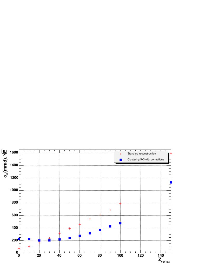
Figure 1: Angular resolution of ATLAS barrel EM calorimeter as a function of the position of the production vertex.

This study has shown that standard reconstruction algorithm is not well suited for non-pointing photons and that a specific treatment is necessary. The next step to improve the resolution would be to try other clustering algorithms such as NearestNeighbor. Another possible way would be to study the dissymmetric shower profile of non-pointing photons and try to extract an alternative method for computing $\eta$ barycenter from this information.

3 EFFECT ON THE GAUGE MEDIATION STUDY

First of all, the $\theta$ resolution affects the selection efficiency of non-pointing photons and background contamination from pointing photons. Second, the resolution of the decay kinematics would be reduced if the photon angle resolution is reduced. We study this in terms of the angle $\psi$ defined as the opening angle of the gravitino direction and the photon direction. This can be calculated by using the following formula

$$\cos\psi = \frac{1-\xi^{2}}{1+\xi^{2}}\ ,$$ (3)

$${\rm where}\ \ \xi \equiv \frac{ct_{\gamma}-L\cos\alpha}{L\sin\alpha},$$ (4)

where $t_{\gamma}$ is the photon arrival time at the barrel EM calorimeter, $L$ is the distance between the interaction point (O) and the point where the photon arrives at the EM calorimeter (A) , and $\alpha$ is the angle between the photon momentum and the position vector $\overrightarrow{OA}$. Changing the $\theta$ resolution and keeping all the other resolutions same as those assumed in Ref. [106], we show in Table 1 the resolution of the angle $\psi$ for point G1 with $c\tau=100$ cm and $\int{\cal L}dt=13.9$ fb^-1.

$\sigma_{\theta}({\rm mrad})\times\sqrt{E({\rm GeV})}$	0	60	100	200	300	400	500
$\sigma_{\psi}$(mrad)	36.5	38.2	40.6	46.9	52.6	56.6	60.2
RMSψ (mrad)	46.2	48.0	50.9	63.0	78.8	93.0	105.5

Table 1: Resolution of the angle $\psi$ for various asumptions of $\theta$ resolution.

Here, $\sigma_{\psi}$ is obtained by Gaussian fit using center part of $\Delta\psi(\equiv\psi-\psi_{\rm true})$ distribution, while RMS_ψ is obtained using the whole distribution. The error $\sigma_{\psi}$ increases as $\sigma_{\theta}$ increases. This affects the error of the $\tilde{\chi}^{0}_{1}$ mass determination.

Part XII Measuring Neutrino Mixing Angles At LHC

W. Porod and P. Skands

1 INTRODUCTION

Recent neutrino experiments [109, 110, 111, 112] clearly show that neutrinos are massive particles and that they mix. In supersymmetric models these findings can be explained by the usual seesaw mechanism [113, 114, 115]. However, supersymmetry allows for an alternative which is intrinsically supersymmetric, namely the breaking of R-parity. The simplest way to realize this idea is to add bilinear terms to the superpotential $W$:

$$W=W_{\rm MSSM}+\epsilon_{i}\hat{L}_{i}\hat{H}_{u}$$ (1)

For consistency one has also to add the corresponding bilinear terms to soft SUSY breaking which induce small vacuum expectation values (vevs) for the sneutrinos. These vevs in turn induce a mixing between neutrinos and neutralinos, giving mass to one neutrino at tree level. The second neutrino mass is induced by loop effects (see [116, 117, 118] and references therein). The same parameters that induce neutrino masses and mixings are also responsible for the decay of the lightest supersymmetric particle (LSP). This implies that there are correlations between neutrino physics and LSP decays [119, 120, 121, 122].

In this note we investigate how well LHC can measure ratios of LSP branching ratios that are correlated to neutrino mixing angles in a scenario where the lightest neutralino $\tilde{\chi}^{0}_{1}$ is the LSP. In particular we focus on the semi-leptonic final states $l_{i}\mathrm{q}^{\prime}\bar{\mathrm{q}}$ ($l_{i}=e,\mu,\tau$). There are several more examples which are discussed in [120]. In the model specified by Eq. (1) the atmospheric mixing angle at tree level is given by

$$\tan\theta_{\rm atm} = \frac{\Lambda_{2}}{\Lambda_{3}}$$ (2)

$$\Lambda_{i}=\epsilon_{i}v_{d}+\mu v_{i}$$ (3)

where $v_{i}$ are the sneutrino vevs and $v_{d}$ is the vev of $H^{0}_{d}$. It turns out that the dominant part of the $\tilde{\chi}^{0}_{1}$-${\mathrm{W}}$-$l_{i}$ coupling $O^{L}_{i}$ is given by

$$O^{L}_{i}=\Lambda_{i}f(M_{1},M_{2},\mu,\tan\beta,v_{d},v_{u})$$ (4)

where the exact form of $f$ can be found in Eq. (20) of ref. [120]. The important point is that $f$ only depends on MSSM parameters but not on the R-parity violating parameters. Putting everything together one finds:

$$\tan^{2}\theta_{\rm atm}\simeq\left|\frac{\Lambda_{2}}{\Lambda_{3}}\right|^{2}\simeq\frac{BR(\tilde{\chi}^{0}_{1}\to\mu^{\pm}{\mathrm{W}}^{\mp})}{BR(\tilde{\chi}^{0}_{1}\to\tau^{\pm}{\mathrm{W}}^{\mp})}\simeq\frac{BR(\tilde{\chi}^{0}_{1}\to\mu^{\pm}\bar{\mathrm{q}}\mathrm{q}^{\prime})}{BR(\tilde{\chi}^{0}_{1}\to\tau^{\pm}\bar{\mathrm{q}}\mathrm{q}^{\prime})},$$ (5)

where the last equality is only approximate due to possible (small) contributions from three body decays of intermediate sleptons and squarks. The restriction to the hadronic final states of the ${\mathrm{W}}$ is necessary for the identification of the lepton flavour. Note that Eq. (5) is a prediction of the bilinear model independent of the R-parity conserving parameters.

2 NUMERICAL RESULTS

We take the SPS1a mSUGRA benchmark point [30] as a specific example, characterized by $m_{0}=100{{\mathrm{GeV}}}$, $m_{\frac{1}{2}}=250{{\mathrm{GeV}}}$, $A_{0}=-100{{\mathrm{GeV}}}$, $\tan\beta=10$, and $\mathrm{sign}(\mu)=1$. The low–energy parameters were derived using SPheno 2.2 [5] and passed to Pythia 6.3 [16] using the recently defined SUSY Les Houches Accord [19]. The R-parity violating parameters (in $\leavevmode\nobreak\ \mathrm{MeV}$) at the low scale are given by: $\epsilon_{1}=43$, $\epsilon_{2}=100$, $\epsilon_{3}=10$, $v_{1}=-2.9$, $v_{2}=-6.7$ and $v_{3}=-0.5$. For the neutrino sector we find $\Delta m^{2}_{\rm atm}=3.8\cdot 10^{-3}$ eV², $\tan^{2}\theta_{\rm atm}=0.91$, $\Delta m^{2}_{\rm sol}=2.9\cdot 10^{-5}$ eV², $\tan^{2}\theta_{\rm sol}=0.31$. Moreover, we find that the following neutralino branching ratios are larger than 1%:

BR$({\mathrm{W}}^{\pm}\mu^{\mp})=2.2\%$,	BR$({\mathrm{W}}^{\pm}\tau^{\mp})=3.2\%$,	BR$(\bar{\mathrm{q}}\mathrm{q}^{\prime}\mu^{\mp})=1.5\%$,
BR$(\bar{\mathrm{q}}\mathrm{q}^{\prime}\tau^{\mp})=2.1\%$,	BR$(\mathrm{q}\bar{\mathrm{q}}\nu_{i})=4.7\%$,	BR$(\mathrm{b}\bar{\mathrm{b}}\nu_{i})=15.6\%$,
BR$(e^{\pm}\tau^{\mp}\nu_{i})=5.9\%$,	BR$(\mu^{\pm}\tau^{\mp}\nu_{i})=30.3\%$,	BR$(\tau^{+}\tau^{-}\nu_{i})=37.3\%$,

where we have summed over the neutrino final states as well as over the first two generations of quarks. Moreover, there are 0.2% of neutralinos decaying invisibly into three neutrinos. In the case that such events can be identified they can be used to distinguish this model from a model with trilinear R-parity violating couplings because in the latter case they are absent.

We now turn to the question to what extent the ratio, Eq. (5), could be measurable at an LHC experiment. The intention here is merely to illustrate the phenomenology and to give a rough idea of the possibilities. For simplicity, we employ a number of shortcuts; e.g. detector energy resolution effects are ignored and events are only generated at the parton level. Thus, we label a final-state quark or gluon which has $p_{\perp}>15{{\mathrm{GeV}}}$ and which lies within the fiducial volume of the calorimeter, $|\eta|<4.9$, simply as ‘a jet’. Charged leptons are required to lie within the inner detector coverage, $|\eta|<2.5$, and to have $p_{\perp}>5{{\mathrm{GeV}}}$ (electrons), $p_{\perp}>6{{\mathrm{GeV}}}$ (muons), or $p_{\perp}>20{{\mathrm{GeV}}}$ (taus). The assumed efficiencies for such leptons are [79] 75% for electrons, 95% for muons, and 85% for taus decaying in the 3–prong modes (we do not use the 1–prong decays), independent of $p_{\perp}$.

For SPS1a, the total SUSY cross section is $\sigma_{\mathrm{SUSY}}\sim 41\leavevmode\nobreak\ \mathrm{pb}$. This consists mainly of gluino and squark pair production followed by subsequent cascades down to the LSP, the $\tilde{\chi}^{0}_{1}$. With an integrated luminosity of $100\leavevmode\nobreak\ {\mathrm{fb}}^{-1}$, approximately 8 million $\tilde{\chi}^{0}_{1}$ decays should thus have occurred in the detector.

An important feature of the scenario considered here is that the $\tilde{\chi}^{0}_{1}$ width is sufficiently small to result in a potentially observable displaced vertex. By comparing the decay length, $c\tau=0.5$ mm, with an estimated vertex resolution of about 20 microns in the transverse plane and 0.5 mm along the beam axis, it is apparent that the two neutralino decay vertices should exhibit observable displacements in a fair fraction of events. Specifically, we require that both neutralino decays should occur outside an ellipsoid defined by 5 times the resolution. For at least one of the vertices (the ‘signal’ vertex), all three decay products ($\mu\mathrm{q}\bar{\mathrm{q}}^{\prime}$ or $\tau\mathrm{q}\bar{\mathrm{q}}^{\prime}$) must be reconstructed, while we only require one reconstructed decay product (jet in the inner detector or lepton in the inner detector whose track does not intersect the 5$\sigma$ vertex resolution ellipsoid) for the second vertex (the ‘tag’ vertex).

Naturally, since the decay occurs within the detector, the standard SUSY missing $E_{\perp}$ triggers are ineffective. Avoiding a discussion of detailed trigger menus (cf. [123]), we have approached the issue by requiring that each event contains either four jets, each with $p_{\perp}>100{{\mathrm{GeV}}}$, or two jets with $p_{\perp}>100{{\mathrm{GeV}}}$ together with a lepton (here meaning muon or electron) with $p_{\perp}>20{{\mathrm{GeV}}}$, or one jet with $p_{\perp}>100{{\mathrm{GeV}}}$ together with two leptons with $p_{\perp}>20{{\mathrm{GeV}}}$. Further, since the Standard Model background will presumably be dominated by $\mathrm{t}\bar{\mathrm{t}}$ events, we impose an additional parton–level $\mathrm{b}$ jet veto.

To estimate the efficiency with which decays into each channel can be reconstructed, a sample of 7.9 million SUSY events were generated with Pythia, and the above trigger and reconstruction cuts were imposed. To be conservative, we only include the resonant decay channels, where the quark pair at the signal vertex has the invariant mass of the ${W}$. The number of generated decays into each channel, the fractions remaining after cuts, and the expected total number of reconstructed events scaled to an integrated luminosity of $100\leavevmode\nobreak\ {\mathrm{fb}}^{-1}$ are given in table 1.

mode	$N_{gen}$	$\epsilon_{\mathrm{rec}}$	$N_{\mathrm{rec}}(100\leavevmode\nobreak\ {\mathrm{fb}}^{-1})$
$\tilde{\chi}^{0}_{1}\to\mu{W}\to\mu\mathrm{q}\bar{\mathrm{q}}^{\prime}$	235000	0.10	12500
$\tilde{\chi}^{0}_{1}\to\tau{W}\to\tau_{\mathrm{3-prong}}\mathrm{q}\bar{\mathrm{q}}^{\prime}$	51600	0.054	1400

Table 1: Statistical sample, estimated reconstruction efficiencies, and expected event numbers.

The comparatively small efficiencies owe mainly to the requirement that both neutralino decays should pass the 5$\sigma$ vertex resolution cut. Nonetheless, using these numbers as a first estimate, the expected statistical accuracy of the ratio, $R={BR(\tilde{\chi}^{0}_{1}\to\mu^{\pm}{W}^{\mp})}/{BR(\tilde{\chi}^{0}_{1}\to\tau^{\pm}{W}^{\mp})}$, appearing in Eq. (5) becomes $\frac{\sigma(R)}{R}\simeq 0.028$.

3 CONCLUSIONS

We have studied neutralino decays in a model where bilinear R-parity violating terms are added to the usual MSSM Lagrangian. This model can successfully explain neutrino data and leads at the same time to predictions for ratios of the LSP decay branching ratios. In particular we have considered a scenario where the lightest neutralino is the LSP. In this case the ratio ${BR(\tilde{\chi}^{0}_{1}\to\mu^{\pm}{W}^{\mp})}/{BR(\tilde{\chi}^{0}_{1}\to\tau^{\pm}{W}^{\mp})}$ is directly related to the atmospheric neutrino mixing angle. Provided R-parity violating SUSY is discovered, the measurement of this ratio at colliders would thus constitute an important test of the hypothesis of a supersymmetric origin of neutrino masses.

We have investigated the possibility of performing this measurement at a ‘generic’ LHC experiment, using Pythia to generate LHC SUSY events at the parton level and imposing semi-realistic acceptance and reconstruction cuts. Within this simplified framework, we find that the LHC should be sensitive to a possible connection between R-parity violating LSP decays and the atmospheric mixing angle, at least for scenarios with a fairly light sparticle spectrum and where the neutralino decay length is sufficiently large to give observable displaced vertices. Obviously, the numbers presented here represent crude estimates and should not be taken too literally. A more refined experimental analysis would be necessary for more definitive conclusions to be drawn.

ACKNOWLEDGEMENTS

We thank A. De Roeck and T. Sjöstrand for useful discussions. We are also grateful to the NorduGRID project for use of computing resources. W.P. is supported by the ‘Erwin Schrödinger fellowship No. J2272’ of the ‘Fonds zur Förderung der wissenschaftlichen Forschung’ of Austria and partly by the Swiss ‘Nationalfonds’.

Part XIII Resonant slepton production at the LHC in models with an ultralight gravitino

B.C. Allanach, M. Guchait, K. Sridhar

1 INTRODUCTION

This letter is devoted to the study of the signals at the Large Hadron Collider (LHC) due to a supersymmetric generalisation of the Standard Model (SM) which (a) violates $R$-parity, and (b) has an ultra-light gravitino in its spectrum. The anomalous events in the CDF experiment in the production rate of lepton-photon-${\not\!\!E}_{T}$ in $p{\bar{p}}$ collisions were explained [124, 125, 126] in the framework of a $R$-parity violating supersymmetric model with dominant $L$-violating $\lambda^{\prime}_{211}$ coupling, and an ultra-light gravitino of mass $\sim 10^{-3}$ eV.

The resonant production of a smuon via the $R$-violating coupling, its decay into neutralino and a muon and, finally, the decay of the neutralino into a gravitino and a photon leads to the $\mu\gamma{\not\!\!E}_{T}$ final state studied in the CDF experiment. The range of smuon and neutralino masses rel¡evant to the explanation of these anomalous observations of the the CDF experiment is such that most of this range will be explored at the Run II of the Tevatron. In the event that this signal is not seen at Run II it will rule out the model at the lower end of the neutralino and smuon masses. For heavier smuon and neutralino masses (above 250 GeV, roughly), the aforementioned Run I signal would be a statistical fluke and will probably disappear in Run II data. In that case, experiments at the LHC can be expected to discover and measure the sparticles. Here, we perform a study of the ability of the LHC to perform these two tasks, identifying the sensitive observables.

2 THE MODEL

We assume a single dominant $R$ violating coupling, $\lambda^{\prime}_{211}$ for example. If the $R$-violating coupling is small, the existence of an ultralight gravitino in the mass range of $10^{-3}$ eV drastically alters the decay mode of the slepton. The slepton overwhelmingly decays into a lepton and a (bino-dominated) neutralino, with the latter decaying into a photon and a gravitino resulting in a $l\gamma{\not\!\!E}_{T}$ final-state. The Feynman diagram for the process is shown in Fig. 1. We should also expect signals from sneutrino production. The background to the $\gamma{\not\!\!E}_{T}$ final-state that this would give rise to depend crucially on cosmic ray events which are difficult to estimate. Therefore we have not studied the signal from sneutrino production. All sparticles except the neutralino, gravitino and slepton are set to be arbitrarily heavy in our analysis.

Figure 1: Feynman diagram of resonant slepton production followed by neutralino decay.

3 SIMULATION RESULTS

For our study of the process shown in Fig. 1 at the LHC ($pp$ collisions at $\sqrt{s}=14$ TeV), we have chosen to work with the following default set of model parameters (unless indicated otherwise):

• Gravitino mass, $m_{\tilde{G}}=10^{-3}$ eV,

• $R$-violating coupling $\lambda^{\prime}\equiv\lambda^{\prime}_{211}=0.01$,

• ${\rm tan}\beta=10$,

• sparticle masses $(m_{\chi_{1}^{0}},m_{\tilde{l}})$=(120 GeV,200 GeV) or (200 GeV,500 GeV) GeV (“low mass” and “high mass” scenarios) respectively.

The choice of using $\lambda^{\prime}_{211}$ rather than some other flavour combination is arbitrary and can be easily generalised to other $R$-violating couplings. We have checked that the chosen value for $\lambda^{\prime}_{211}$ is quite consistent with the existing bound  [127, 128]. By selecting rather low values for $R$-parity coupling and gravitino mass,we avoid significant rates for the possible $R$-violating decays of $\chi_{1}^{0}\rightarrow\mu jj$ or $\chi_{1}^{0}\rightarrow\nu jj$. $\chi_{1}^{-}\rightarrow\gamma{\tilde{G}}$ is the dominant channel. We use the ISASUSY [129] to generate the SUSY spectrum, branching ratios and decays of the sparticles selecting a representative point $\tan\beta$=10, $A_{t,\tau,b}=0$ along with large values of $\mu$ and other flavour diagonal soft supersymmetry breaking parameters.

The signals have been simulated using HERWIG6.4 [130] and the $W\gamma$ SM background has been simulated using PYTHIA [16]. In our simulations, both the signal and background, we have used only selection cuts of $E_{T},{\not\!\!E}_{T}>25$ GeV on the transverse energies of the muon, the photon and missing energy. We have used the following cuts on the rapidity of the photon and the muon: $|\eta_{\gamma,\mu}|<3$. There is an isolation cut between the photon and other hard objects $o$ in the event of $\sqrt{(\eta_{\gamma}-\eta_{o})^{2}+(\phi_{\gamma}-\phi_{o})^{2}}>0.7$. Since the signal is hadronically quiet, we veto events with jets reconstructed with $E_{T}>30$ GeV and $\eta_{j}<4$. Initial and final state radiation effects, as well as fragmentation effects are included in the background simulation.

Figure 2: $M_{T}$ distributions of (a) $\mu\gamma{\not\!\!E}_{T}$, (b) $\gamma{\not\!\!E}_{T}$ for slepton. 300 fb^-1 integrated luminosity at the LHC is assumed. The purple (lighter) histograms display $W\gamma$ SM background, the red (darker) histograms show signal plus background for $(m_{\chi_{1}^{0}},m_{\tilde{l}})$=(120 GeV,200 GeV), whereas the blue (dotted) histograms display the signal plus background distributions for $(m_{\chi_{1}^{0}},m_{\tilde{l}})$=(200 GeV,500 GeV). In (a), the dashed black line displays a log-linear fit to the background distribution for $M_{T}=150-400$ GeV. In (b), the insert shows a linear scale magnification of an area of the plot.

The transverse mass distributions of final state particles along with ${\not\!\!E}_{T}$ show a clear distinction between signal and backgrounds. The $M_{T}(\mu\gamma{\not\!\!E}_{T})$ and $M_{T}(\gamma{\not\!\!E}_{T})$ distributions are displayed in Figs. 2a,b for the simulated high and low mass points and $W\gamma$ simulated SM background. In Fig. 2a, sharp peaks which are expected in the $M_{T}(\mu\gamma{\not\!\!E}_{T})$ distributions are clearly visible at values of the smuon mass and will be detected above the SM $W\gamma$ background, leading to the accurate measurement of the mas. Fig. 2b shows that the signal peaks in $M_{T}(\gamma{\not\!\!E}_{T})$ (predicted to be at the neutralino mass) should be able to provide a measurement of the neutralino mass.

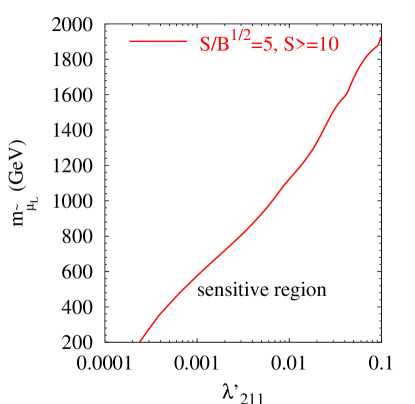
Figure 3: Search reach for the $\mu\gamma{\not\!\!E}_{T}$ signal (as defined in the text) for 300 fb^-1 integrated luminosity at the LHC.

In order to calculate the search reach, we use the signal $S$ in the 4 highest peak bins (covering 20 GeV) of the signal $M_{T}(\mu\gamma{\not\!\!E}_{T})$ peak. The background distribution in these four bins is estimated by fitting a simple function B = 4 $\mbox{exp}\left[aM_{T}(\mu\gamma{\not\!\!E}_{T})+b\right]$ to $M_{T}(\gamma\mu{\not\!\!E}_{T})$ between 150-400 GeV in Fig. 2a. Using purely $\sqrt{B}$ statistical errors, we obtain to $a=-0.018\pm 0.001$, $b=9.25\pm 0.22$. $B$ is displayed in Fig. 2a as the dashed black line. We show the region of parameter space corresponding to $S/\sqrt{B}>5$ and $S\geq 10$ for 300 fb^-1 luminosity option, as a function of smuon mass and R-parity conserving coupling in Fig. 3a.

We now turn to the decay ${\tilde{l}}\rightarrow{\tilde{G}}l$. We ignore sneutrino production in this case because it would lead to an invisible final state. We have calculated the production matrix element and the branching ratio and implemented in a parton-level Monte Carlo. We have used cuts in our analysis on the muon and missing transverse energy identical to the $\gamma\mu{\not\!\!E}_{T}$ analysis, i.e. ${\not\!\!E}_{T},E_{T}^{\mu}>25$ GeV and $|\eta_{\mu}|<3$.

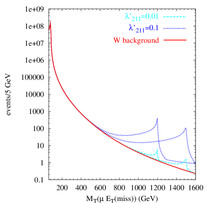
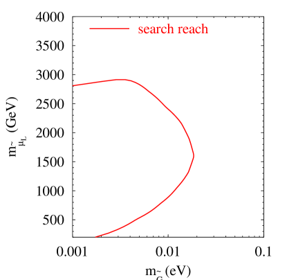
Figure 4: (a) $M_{T}$ distribution of the $\mu{\tilde{G}}$ final state for two different values of the smuon mass and 300 fb^-1 integrated luminosity at the LHC. The left(right)-most three peaks are for smuon masses of 1.2 TeV and 1.5 TeV respectively. (b) Search reach (as defined in the text) for the $\mu\tilde{G}$ final state and 300 fb^-1 integrated luminosity at the LHC and $\lambda^{\prime}_{211}=0.1$. The search reach is contained to the left of the curve.

Fig. 4a displays the $M_{T}(\mu{\not\!\!E}_{T})$ distribution for the $W$ background plus signal in the cases $m_{\tilde{\mu}}=1.2$ and 1.5 TeV respectively and two different values of the $\lambda^{\prime}$. For $\lambda^{\prime}=0.01$ there are not enough signal events to be seen, but for higher values (eg 0.1), a clear mass peak should be seen in the tail of the $M_{T}$ distribution of the $W$. We define the search reach by the criteria that for $S$ signal and $B$ background events, $S/\sqrt{B}\geq 5$ and $S\geq 10$ in the 5 GeV signal peak bin of $M_{T}(\mu{\not\!\!E}_{T})$. It is displayed for 300 fb^-1 of integrated luminosity in Fig. 4b.

CONCLUSIONS

Resonant slepton production and its decays into $l\gamma{\tilde{G}}$ or $l{\tilde{G}}$ can be discovered at the LHC for slepton masses into the multi-TeV region, depending upon the $R_{p}$ violating coupling and provided that the gravitino is ultra-light (with a mass less than 0.1 eV). Various $M_{T}$ distributions will allow the accurate measurement of sparticle masses involved. For full details, the new matrix element and additional results (for example including the case of a smuon NLSP), see ref. [131].

ACKNOWLEDGEMENTS

K Sridhar would like to thank CERN and LAPTH for hospitality offered during which some of the work contained herein was performed.

Part XIV Radion Mixing Effects In The Two-Higgs-Doublet Model

J.L. Hewett and T.G. Rizzo

1 INTRODUCTION

The RS model[132] provides an interesting solution to the hierarchy problem which can be tested experimentally[133, 134, 135] at future colliders. One prediction of this model is the existence of a relatively light scalar radion which can mix with other scalars such as the Higgs boson of the Standard Model (SM). Such mixing can lead to substantial modifications in the expected properties of both the Higgs and the radion and has been extensively studied[136, 137, 138, 139] in the literature. Here we extend this study to the case of two Higgs doublets as would be expected in a number of scenarios, $e.g.$, supersymmetry (SUSY). Although not necessary for solving the hierarchy problem within the RS scenario, SUSY may have other model building[140, 141] uses such as coupling constant unification or radius stabilisation[142]. The expectation from previous analyses of the single doublet model is that the properties of the mass eigenstate CP even neutral fields would substantially differ from those predicted in either the SM or the Minimal Supersymmetric Standard Model (MSSM). The preliminary discussion of our findings given here supports these expectations though further study is required to understand the breath of the possible modifications.

2 ANALYSIS

With two Higgs doublets, mixing arises from the TeV brane action

$$S_{mix}=\int_{TeV}d^{4}x{\sqrt{det\leavevmode\nobreak\ g}}\leavevmode\nobreak\ R(g)\leavevmode\nobreak\ (\xi_{1}H_{1}^{\dagger}H_{1}+\xi_{2}H_{2}^{\dagger}H_{2}+\xi_{12}H_{1}^{\dagger}H_{2}+h.c.)\,,$$ (1)

where $g$ symbolises the induced metric on the TeV brane, $R$, the induced curvature arising from $g$, $H_{i}$ are the two Higgs doublets and $\xi_{i}$ are dimensionless, order one parameters which we take to be real, thus assuming CP conservation for simplicity. The possible complexity of $\xi_{12}$ may lead to interesting phenomenology. (In what follows $\xi_{1}=\xi_{2}$ will be assumed since it is unlikely that gravitational interactions distinguish between these two Higgs doublets. This assumption, however, may be incorrect.) Thus, in the unitary gauge, the CP-odd field, $A$, as well as the charged scalars $H^{\pm}$ are not directly affected by modifications to the neutral CP even sector. (Of course, their couplings to the CP-even fields will be modified.) Before mixing with the radion, $r_{0}$, we denote the usual two CP-even Higgs by $h_{0},H_{0}$ which have been obtained from the weak interaction eigenstate fields via rotations by the angles $\alpha,\beta$ as usual. Assuming $r_{0}$ obtains a mass from the stabilisation procedure, the above action can be expanded to quadratic order in the CP-even neutral fields from which one obtains the following effective Lagrangian generalising the notation of Csaki $etal.$[137]:

$${\cal L}=-{1\over{2}}h_{0}\partial^{2}h_{0}-{1\over{2}}m_{h_{0}}^{2}h_{0}^{2}\leavevmode\nobreak\ +(h_{0}\rightarrow H_{0},r_{0})-3\sigma\gamma^{2}r_{0}\partial^{2}r_{0}+6\gamma(\tau_{h}h_{0}\partial^{2}r_{0}+h_{0}\rightarrow H_{0})\,,$$ (2)

where $\gamma=v/\sqrt{6}\Lambda_{\pi}\sim 0.05-0.10$, with $v$ the SM vev, and $\Lambda_{\pi}$, of order a few TeV or so, being the ‘TeV scale’ of the RS model. The parameters $\sigma,\tau_{h,H}$ are functions of the $\xi_{i}$ and the usual mixing angles $\alpha,\beta$. The kinetic mixing in the above Lagrangian can be removed by a set of field redefinitions, $i.e.$, $h_{0},H_{0}\rightarrow h^{\prime},H^{\prime}+6\gamma\tau_{h,H}r^{\prime}/Z$ and $r_{0}\rightarrow r^{\prime}/Z$. To obtain the mass eigenstate basis after the above redefinitions are employed a further orthogonal transformation, $(h^{\prime},H^{\prime}r^{\prime})={\cal O}(h,H,r)$, must be performed. The elements of the orthogonal matrix, $\cal O$, as well as the corresponding mass eigenvalues can then be determined analytically.

 

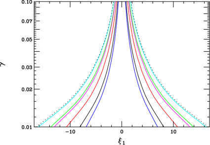
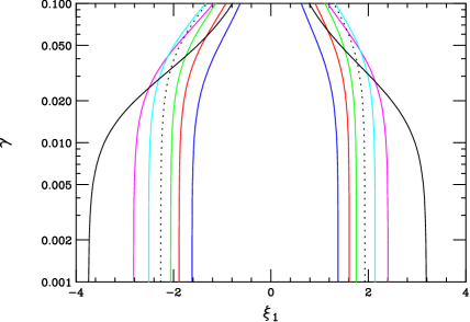
Figure 1: Constraints from the absence of ghosts/tachyons(left) and perturbative unitarity(right) for different values of the ratio $R$ in the range between -2 and +2. The allowed region lies between the curves.

The number of parameters in this model is unfortunately rather large making it difficult to analyse in all generality. In order to show a specific example with somewhat fewer parameters we assume that the spectra, couplings, $etc.$, of the unmixed two-doublet-model Higgs sector to be that given by SUSY, including the effects of radiative corrections[143], with $\tan\beta=10$, $M_{A}=500$ GeV, $A_{t}=A_{b}=-\mu$=1 TeV and $M_{S}^{2}=(M_{t_{1}}^{2}+M_{t_{2}}^{2})/2=1$ TeV² where the $M_{t_{i}}$ are the stop masses. (The remaining parameters are $\xi_{1},m_{r_{0}},\gamma$ and the ratio $R=\xi_{12}/\xi_{1}$.) These parameter choices yield $m_{h}\simeq 125$ GeV. The resulting parameter space can be further restricted by noting that both $\xi_{1}$ and $R$ are of order unity, $\gamma$ is anticipated to be near the range described above and $m_{r_{0}}$ is expected to be of order the weak scale. Further numerical restrictions on the parameter ranges can be obtained by demanding that, $e.g.$, there are no ghosts or tachyons in the spectrum arising from the diagonalisation process and that $W_{L}^{+}W_{L}^{-}$ scattering satisfies perturbative unitarity[144] up to the scale $\Lambda_{\pi}$; samples of such constraints can be seen in the figure above where we have assumed that $-2\leq R\leq 2$. Note that for small values of $\gamma$ the constraints from unitarity are more restrictive than the requirement that no ghosts or tachyons be present; for larger $\gamma$ both constraints are found to be of comparable strength.

3 PRELIMINARY RESULTS

We now turn to a brief sample of our results which survey only a Small region of the allowed parameter space. The first thing to examine is the effect of mixing on the masses of the physical states $h,H,r$ as is shown in the next set of figures. (The curves are cut off at large values of $|\xi_{1}|$ by the no ghost/tachyon requirement.) Here we see the typical result that the mass ‘levels’ of the three states repel each other due to mixing. In all of our examples, $m_{H_{0}}$ is the largest mass parameter and thus the mass of the $H$ is itself raised by mixing. Note that these upward shifts can be enormous near the parameter space boundaries. Though made heavier, $H$’s couplings will be seen to grow as well. When $m_{h_{0}}<(>)m_{r_{0}}$ we see that the $h(r)$ mass is pushed downward while that of $r(h)$ is pushed upward. These shifts are not as large as those experienced by the $H$. Thus while we might expect the light Higgs to have a mass $\leq 130$ GeV in the MSSM, mixing with the radion allows it to be larger provided the radion itself is less massive.

 

 

 

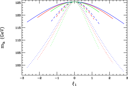
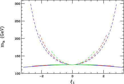
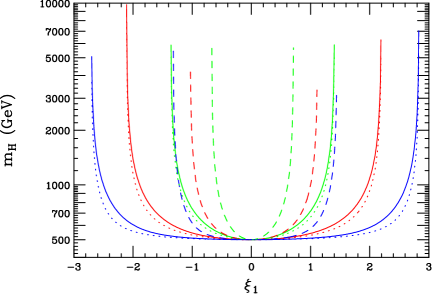
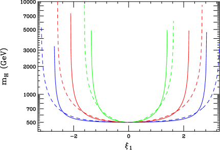
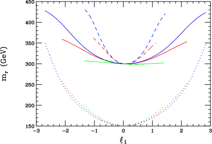
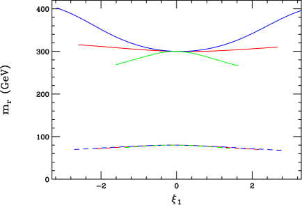
Figure 2: Typical shifts in light Higgs(top), heavy Higgs(middle) and radion(bottom) masses due to mixing for different values of the model parameters. Figures in a given column are case correlated.

Next we consider the shifts due to mixing in the squares of the couplings of the various fields to either $b\bar{b}$ or $t\bar{t}(c\bar{c})$; it is important to note that the corresponding shifts for the couplings to $WW/ZZ$ are found to almost identical to those for $b\bar{b}$ in almost all cases so we do not present those results separately here. Note that we have scaled these couplings shown in the figures either by their value in the MSSM using the input parameters above, as in the case of $h,H$, or by their unmixed values, as in the case of $r$. The range of coupling shifts, especially for $H$ and $r$, are truly impressive being orders of magnitude in some cases. Not only are large enhancements seen for some parameter ranges, it is also important to note that there are regions of the parameter space, not necessarily near the boundaries, where couplings can completely vanish. For the light Higgs we see that while the mixing effects are not as large, for the cases at hand they always lead to a reduction in the coupling strengths in comparison with MSSM expectations.

 

 

 

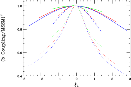
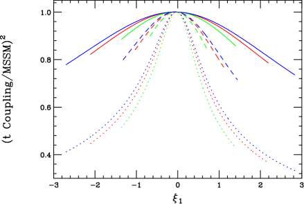
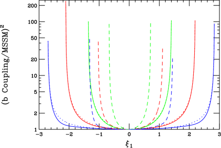
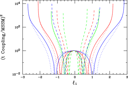
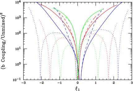
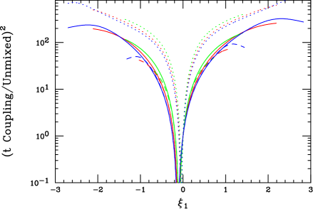
Figure 3: Typical shifts in light Higgs(top), heavy Higgs(middle) and radion(bottom) couplings to $b\bar{b}$(left) and $t\bar{t}$(right) due to mixing for different values of the model parameters. Figures are correlated in a given column.

For the light Higgs, $h$, it is particularly important to examine the variations in the couplings to the $gg$ and $\gamma\gamma$ final state since these control the dominant signal rate at the LHC; these are shown in the next set of figures. While the couplings of $h$ to quarks and massive vector bosons was generally reduced via mixing, we see here that the loop-induced processes can be either enhanced or suppressed depending upon the region of parameter space we happen to be sitting in. The shift in the couplings of $H,r$ to $gg$ and $\gamma\gamma$ will be presented elsewhere.

 

 

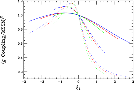
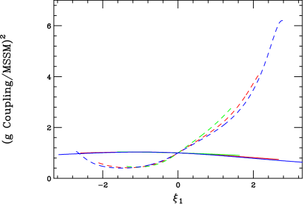
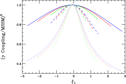
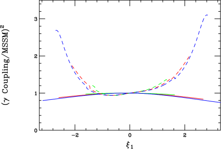
Figure 4: Shifts in $gg$(top) and $\gamma\gamma$(bottom) couplings of the $h$ due to mixing. Figures in a given column are correlated.

4 CONCLUSIONS

We have begun a preliminary examination of the effects of mixing between the radion and the two CP even Higgs fields present in the two-doublet-model. As a result of this mixing the masses and couplings of all of these fields are found to be substantially modified from the expectations of the MSSM. Further analysis into the details of these mixing effects and the corresponding shifts in the various particle widths is on-going.

Part XV Search For The Radion Decay $\phi\rightarrow\rm h\rm h$ With $\gamma\gamma$+$\rm b\bar{\rm b}$, $\tau\tau$+$\rm b\bar{\rm b}$ And $\rm b\bar{\rm b}$+$\rm b\bar{\rm b}$ Final States In CMS

D. Dominici, G. Dewhirst, S. Gennai, L. Fan$\grave{o}$, A. Nikitenko

1 INTRODUCTION

The Randall Sundrum model (RS) [132, 145] has recently received much attention because it could provide a solution to the hierarchy problem, by means of an exponential factor in a five dimensional non-factorizable metric. In the simplest version the RS model is based on a five dimensional universe with two four dimensional hypersurfaces (branes), located at the boundary of the fifth coordinate $y$. By placing all the Standard Model fields on the visible brane at $y=1/2$ all the mass terms, which are of the order of the Planck mass, are rescaled by the exponential factor, to a scale of the order of a TeV. The fluctuations in the metric in the fifth dimension are described in terms of a scalar field, the radion which in general mixes with the Higgs. This scalar sector of the RS model is parametrized in terms of a dimensionless parameter $\xi$, of the Higgs and radion masses $m_{h}$, $m_{\phi}$ and the vacuum expectation value of the radion field $\Lambda_{\phi}$. The phenomenology of the Higgs and radion at LHC has been the object of several studies [136, 146, 138, 139, 147, 148] concentrating mainly on Higgs and radion production. In general the Higgs and radion detection is not guaranteed in all the parameter space region. The presence in the Higgs radion sector of trilinear terms opens up the important possibility of $\phi\to hh$ decay and ${\rm h}\to\phi\phi$. For example for $\rm m_{\rm h}=120$ GeV/$c^{2}$, $\Lambda_{\phi}=5$ TeV and $\rm m_{\phi}\sim 250-350$ GeV/$c^{2}$ the $BR(\phi\to\rm hh)\sim 0.2-0.3$. In this paper we estimate the CMS discovery potential for the radion ($\phi$) in two Higgs decay mode ($\phi\rightarrow\rm h\rm h$) with $\gamma\gamma$+$\rm b\bar{\rm b}$, $\tau\tau$+$\rm b\bar{\rm b}$ and $\rm b\bar{\rm b}$+$\rm b\bar{\rm b}$ final states.

2 ANALYSIS

One point of $\rm m_{\phi}$=300 GeV/$c^{2}$ and $\rm m_{\rm h}$=125 GeV/$c^{2}$ was taken and the observability in the ($\xi$, $\Lambda_{\phi}$) plane was evaluated. Signal events were simulated with the PYTHIA [149] MSSM $\rm g\rm g\rightarrow\rm H\rightarrow\rm h\rm h$ process when values of $\rm m_{\rm H}$ and $\rm m_{\rm h}$ were set to 300 and 125 GeV/$c^{2}$. $\Gamma_{\rm H}$ was set to $\sim$ 1 GeV/$c^{2}$, thus the variation of the radion width in the ($\xi$, $\Lambda_{\phi}$) plane was neglected. However, the effect of changing of the radion width will be not visible due to the fact that $\Gamma_{\phi}$ is small in comparison with the detector resolution when the radion mass is reconstructed.

2.1 $\gamma\gamma\rm b\bar{\rm b}$ final state

Signal events were processed with the full detector simulation and reconstruction. Events were required to pass the Level-1 and High Level Trigger (HLT) selections for the di-photon stream  [150, 151] with HLT thresholds on photons of 40 and 25 GeV/$c$. Photons were required to be isolated with the tracker and the electromagnetic calorimeter. The two highest $\rm E_{\rm T}$ jets of $\rm E_{\rm T}>$ 30 GeV and $|\eta|<$2.4 were reconstructed with the calorimeter and were taken as b-jet candidates from $\rm h\rightarrow\rm b\bar{\rm b}$ decay. At least one of these two jets has to be tagged as a b jet. The efficiency of single b tagging is 0.61 per event. Further selections require the di-jet mass, $\rm M_{\rm b\rm j}$, to be in the window $\rm m_{\rm h}\pm$ 30 GeV/$c^{2}$ (efficiency 65 %) and the di-photon mass, $\rm M_{\gamma\gamma}$, to be in the window $\rm m_{\rm h}\pm$ 2 GeV/$c^{2}$ (efficiency 78 %). Finaly, the $\rm M_{\gamma\gamma\rm b\rm j}$ mass should be in the window of $\rm m_{\phi}\pm$ 50 GeV/$c^{2}$ (efficiency 95 %). Figure 1 shows $\rm M_{\rm b\rm j}$ and $\rm M_{\gamma\gamma\rm b\rm j}$ distributions with arbitrary normalization after selections. The signal efficiency of the whole selection chain is 3.7 %. For $\Lambda_{\phi}$ = 1 TeV and $\xi$ = 0 the expected number of signal events with 30 fb^-1 is 41 (with $\sigma$($\rm g\rm g\rightarrow\phi$) = 40.8 pb, Br($\phi\rightarrow\rm h\rm h$) = 0.33, Br($\rm h\rightarrow\rm b\bar{\rm b}$) = 0.61, Br($\rm h\rightarrow\gamma\gamma$) = 0.00225).

Figure 1: Reconstructed b j (left) and $\gamma\gamma\rm b\rm j$ mass for the signal.

Irreducible di-photon backgrounds were generated with CompHEP [14] for the $\gamma\gamma\rm j\rm j$ (j=u,d,s,g) process and with MadGraph [152, 153] for the $\gamma\gamma\rm c\bar{\rm c}$ and $\gamma\gamma\rm b\bar{\rm b}$ processes with the factorization and the renormalization scales set to $\rm M_{\rm Z}$ and CTEQ5L PDF. The generator level preselections are $\rm p_{\rm T,\rm max\leavevmode\nobreak\ (\rm min)}^{\gamma}>$35 (20) GeV/$c$, $\rm p_{\rm T}^{\rm j}>$20 GeV/$c$, $|\eta|<$2.5, $\Delta\rm R_{\gamma\gamma}>$0.3, $\Delta\rm R_{\gamma\rm j}>$0.3, $\Delta\rm R_{\rm j\rm j}>$0.3. Cross sections are shown in Table 1. PYTHIA was used for the hadronization. Initial and final state radiation in PYTHIA (ISR, FSR) were switched on. A fast detector simulation with the realistic resolution of the photon and jet energies and track momentum was used. The track reconstruction efficiency of 0.9 was taken into account in the tracker isolation criteria. The efficiency of b tagging, 0.5, for b jets and the mistagging probability of 0.01 (0.1) for u,d,s,g (c) jets were used. These numbers correspond to what was obtained with the full detector simulation  [154] using the impact parameter tagging method. The efficiency of the selections and the expected number of the background events with 30 fb^-1 after all selections including b tagging are shown in Table 1. Statistical errors on the expected number of events are also shown. The number of background events was then multiplied by 0.92 and by 0.90 to take into account of the Level-1 e/$\gamma$ trigger and the calorimeter isolation efficiencies which were not taken into account in the fast simulation. These efficiencies were obtained from a full simulation of the signal events.

Table 1: Background cross sections, efficiency, number of events with 30 fb^-1 after all selections including b tagging.

	$\gamma\gamma\rm j\rm j$	$\gamma\gamma\rm c\bar{\rm c}$	$\gamma\gamma\rm b\bar{\rm b}$
cross-section, fb	13310	778	76
selections	efficiency
$\rm E_{\rm T}^{\gamma_{1,2}}>$ 40, 25 GeV, $|\eta|<$ 2.5	0.446	0.466	0.487
tracker isolation in cone 0.3	0.328	0.345	0.379
two jets $E_{\rm T}>$ 30 GeV, $|\eta|<$2.4	0.127	0.125	0.133
$\rm M_{\gamma\gamma}$ window 4 GeV/$c^{2}$	0.00278	0.00263	0.00410
$\rm M_{\rm j\rm j}$ window 60 GeV/$c^{2}$	0.00086	0.00096	0.00144
$\rm M_{\gamma\gamma\rm j\rm j}$ window 100 GeV/$c^{2}$	0.00045	0.00061	0.00123
N events after all selections including b tagging	4.2 $\pm$ 0.8	2.0 $\pm$ 0.6	2.0 $\pm$ 0.6

The CMS discovery reach was obtained in the ($\xi$, $\Lambda_{\phi}$) plane. Figure 2 (left plot) shows the 5 $\sigma$ discovery contour in the the ($\xi$, $\Lambda_{\phi}$) plane when the irreducible background only (6.9 events with 30 fb^-1) was taken into account. Theoretically excluded regions are also shown in the plot. Dashed line contours present the discovery reaches when the irreducible background cross sections were calculated for the renormalization and factorization scales set to 0.5$\times\mu_{\rm 0}$ and to 2$\times\mu_{\rm 0}$, where $\mu_{\rm 0}$ = $\rm M_{\rm Z}$. The background cross section uncertainty due to the scale variation found to be of $\simeq$ 40 % for $\gamma\gamma\rm b\bar{\rm b}$. It was guessed that the cross section variation for $\gamma\gamma\rm c\bar{\rm c}$ and $\gamma\gamma\rm j\rm j$ production may be only slightly different, thus 40 % variation was applied to the cross sections of $\gamma\gamma\rm c\bar{\rm c}$ and $\gamma\gamma\rm j\rm j$ processes as well.

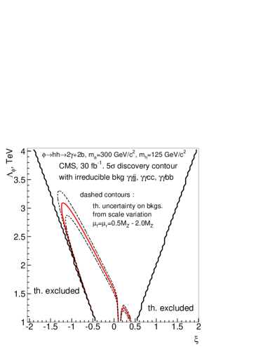
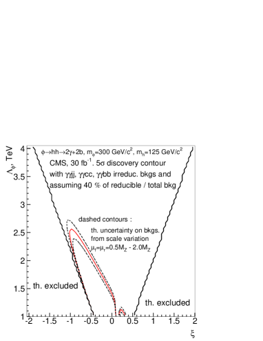
Figure 2: 5 $\sigma$ discovery contours for $\phi\rightarrow\rm h\rm h\rightarrow\gamma\gamma$+$\rm b\bar{\rm b}$ channel ($\rm m_{\phi}$=300 GeV/$c^{2}$, $\rm m_{\rm h}$=125 GeV/$c^{2}$); Left plot : with the irreducible background only; Right plot : with the total background assuming the ratio of the reducible to the total background of 0.4. Dashed line contours present the discovery reaches when the irreducible background cross sections were calculated for the renormalization and factorization scales set to 0.5$\times\mu_{\rm 0}$ and to 2$\times\mu_{\rm 0}$ where $\mu_{\rm 0}$ = $\rm M_{\rm Z}$.

Reducible backgrounds from $\gamma$ + three jets and four-jet processes still have to be evaluated. It is expected from the inclusive $\rm h\rightarrow\gamma\gamma$ studies that the reducible background will be about of 40 % of the total background, thus the total background is expected to be of 11.5 events with 30 fb^-1. Figure 2 (right plot) shows the 5 $\sigma$ discovery contours in the the ($\xi$, $\Lambda_{\phi}$) plane with the total background taken into account. The experimental systematics uncertainty of the background estimated as $\simeq$ 5 % hardly affects the discovery reach due to the signal to background ratio in the 5 $\sigma$ region of the ($\xi$, $\Lambda_{\phi}$) plane is bigger than two.

2.2 $\tau\tau\rm b\overline{\rm b}$ final state

The signature when one $\tau$ lepton decays leptonically and another $\tau$ lepton decays hadronically (producing a $\tau$ jet) was considered. The highest signal cross section times the branching ratios of 0.96 pb was obtained for $\xi$ = $-$0.35 and $\Lambda_{\phi}$ = 1 TeV. The background processes considered in the analysis are shown in Table 2 with the NLO cross sections taken from [155, 156, 157].

Table 2: Trigger and total efficiency for the signal and the backgrounds; expected number of events with 30 fb^-1.

		efficiency (%)		number of
samples	$\sigma\times BR$ (pb)	trigger	trigger + off-line	events
$\phi\rightarrow\tau\tau\rm b\overline{\rm b}$	0.96	6 $\pm$ 0.2	0.35 $\pm$0.06	102
$\rm t\overline{\rm t}\rightarrow\rm l+\nu+jets+\rm b\overline{\rm b}$	180	0.57 $\pm$ 0.02	(1.6 $\pm$0.2)$\times 10^{-3}$	111
$\rm t\overline{\rm t}\rightarrow\rm l+\nu+\tau\leavevmode\nobreak\ \rm jet+\rm b\overline{\rm b}$	15	3.1 $\pm$ 0.2	(7.7 $\pm$ 0.3)$\times 10^{-3}$	66
$\rm Z\rm b\overline{\rm b}\rightarrow\tau\tau+\rm b\overline{\rm b}$	5.4	1.4 $\pm$ 0.2	0.009$\pm$0.003	21
$\rm Z+jets\rightarrow\tau\tau+jets$	306	0.35 $\pm$ 0.02	(3.3 $\pm$ 0.5)$\times 10^{-4}$	36
$\rm W+jets\rightarrow\rm l+\nu+jets$	175	0.039 $\pm$ 0.002	0	0

Background Z+jets (W+jets) were generated with $\hat{\rm p}_{\rm T}>$ 20 (80) GeV/$c$. Signal events were processed with the full detector simulation and reconstruction, while the background was processed with the fast detector simulation package CMSJET [158]. The combined electron(muon)-plus-$\tau$ jet trigger [151] was used in this analysis. The Level-1 trigger threshold is 21 GeV for electrons and 45 GeV for the $\tau$ jet. The inclusive muon threshold is low enough (14 GeV/$c$) to allow a good efficiency however, to increase the background rejection a $\tau$ jet with $\rm E_{\rm T}>$35 GeV is required at the Level-1 trigger. The trigger efficiency is shown in Table 2 for the signal and background samples. Missing transverse momentum and b tagging were used to reconstruct $\tau$ leptons and to identify $\rm b$ jets coming from the two Higgs bosons. In order to increase the signal statistics it was necessary to tag at least one jet. The off-line selections are the following:

• $\Delta\phi$ between lepton and $\tau$ jet direction $>$0.1;

• $\rm E_{\rm T}$ of the $\rm b$-tagged jets $>$30 GeV, and $\rm E_{\rm T}$ of the most energetic jet $>$ 55 GeV;

• transverse mass of the lepton and missing momentum $<$ 35 GeV/$c^{2}$;

• 75 $<\rm M_{\tau\tau}<$165 GeV/c², 100 $<\rm M_{\rm b\rm j}<$150 GeV/c², 265 $<\rm M_{\tau\tau\rm b\rm j}<$ 350 GeV/c².

Table 2 shows the signal and the background efficiencies for the off-line selections and the number of the expected events with 30 fb^-1. Figure 3 shows the reconstructed $\tau\tau\rm b\overline{\rm b}$ mass after all selections (left plot). The total number of the background events after all selections is 234 with 30 fb^-1. The biggest background is $\rm t\bar{\rm t}$ (177 events) while the $\rm W+jets$ background is negligible. Estimating also the contribution of $\rm t\bar{\rm t}$ when both W bosons decay into $\tau$ the total number of background events increases up to 254. For the maximal signal cross section of 0.96 pb, ($\xi$= $-$0.35 and $\Lambda_{\phi}$ = 1 TeV) about 102 signal events are expected. Signal significance ($\rm S/\sqrt{\rm B}$) at this point is 6.4. Figure 3 (right plot) shows a 5 $\sigma$ discovery contour in the ($\xi$, $\Lambda_{\phi}$) plane.The two contours correspond to the uncertainties of the background cross section values at NLO due to the scale variation and different PDFs [155, 156, 157]. The experimental systematics uncertainty of 3 % for the total background was taken into account.

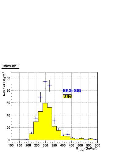
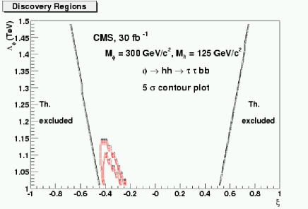
Figure 3: Reconstructed $\tau\tau\rm b\rm j$ mass for the signal and background (left) and 5 $\sigma$ discovery contour (right).The two contours correspond to the maximum and minimum k-factor value derives from the NLO order calculation of background cross section.

2.3 $\rm b\bar{\rm b}\rm b\bar{\rm b}$ final state

The signal cross section times branching ratios for the $\rm g\rm g\rightarrow\phi\rightarrow\rm h\rm h\rightarrow\rm b\bar{\rm b}\rm b\bar{\rm b}$ process is 10.3 pb for $\Lambda_{\phi}$ = 1 TeV and $\xi$ = $-$ 0.35 The main QCD multi-jet background was generated by PYTHIA in different $\hat{\rm p}_{\rm T}$ bins. Other backgrounds considered are $\rm t\bar{\rm t}$, $\rm t\bar{\rm t}\rm j\rm j$ and $\rm Z\rm b\bar{\rm b}$. In Table 3 cross sections and expected numbers of events with 30 fb^-1 are summarized.

Table 3: Signal and background events with 30fb^-1.

	cross section	events in 30 fb-1
Signal	10.3 pb	$3.1\times 10^{5}$
QCD${}_{\hat{\rm p}_{\rm T}(30-170)}$	0.2257 mb	$6.79\times 10^{12}$
$\rm t\bar{\rm t}$	615 pb	$1.8\times 10^{7}$
$\rm t\bar{\rm t}$jj	507 pb	$1.5\times 10^{7}$
$\rm Z\rm b\bar{\rm b}$	349 pb	$1.0\times 10^{7}$

A rejection factor on background higher than $10^{6}$ is needed to reach a 5$\sigma$ statistical evidence of the signal. A fast detector simulation with the CMSJET package  [158] was used for both signal and background samples. Dedicated trigger selections were developed to keep the QCD multi-jet background rate at the acceptable level whilst maintaining a high efficiency for the signal. At Level-1 multi-jet triggers were used with the thresholds taken from Table 15-13 presented in [151] and restricted in pseudorapidity, $|\eta|<$0.8. At the High Level Trigger at least 4 jets were required within the restricted pseudorapidity range, $|\eta|<$0.8. Two jets must be b-tagged with the impact parameter tagging method (2 associated tracks with significance on the transverse impact parameter $>$ 2). The output QCD rate after these selections is $\sim$ 5 Hz. In off-line selections all possible di-jet invariant masses were calculated from the 4 highest $\rm E_{\rm T}$ jets. The two jet pairs were chosen minimizing the value of $\rm m_{i,j}$-$\rm m_{k,l}$, the same jets were then used to reconstruct the radion mass. The mean values (and $\sigma_{\rm fit}$) of the di-jet and four-jet effective masses reconstructed in this way are: 120 (39) GeV/$c^{2}$ and 313 (76) GeV/$c^{2}$. A 1.5 $\sigma$ window in mass around $\rm m_{\rm h}$ and $\rm m_{\phi}$ was used to select signal and background events. Efficiencies for the signal, background and the expected number of events with 30 fb^-1 are summarized in Table 4.

Table 4: Trigger and total selection efficiency and expected number of events with 30 fb^-1

	$\epsilon_{\rm trigger}$	$\epsilon_{\rm total}$	events
signal	0.038	0.031	9.57${}^{.}10^{3}$
QCD $\hat{\rm p}_{\rm T}(80-120)$	$1^{.}10^{-5}$	$7^{.}10^{-6}$	$7.5^{.}10^{5}$
QCD $\hat{\rm p}_{\rm T}(120-170)$	$1^{.}10^{-4}$	$6.6^{.}10^{-5}$	$1.1^{.}10^{6}$
$\rm t\bar{\rm t}$	0.015	0.010	$1.84^{.}10^{5}$
$\rm t\bar{\rm t}$jj	0.056	0.026	$1.8^{.}10^{5}$
$\rm Z\rm b\bar{\rm b}\rightarrow$ 4b	0.002	8${}^{.}10^{-4}$	$1.2^{.}10^{3}$

The di-jet and four-jet invariant mass for the background and the signal at $\Lambda_{\phi}$ = 1 TeV and $\xi$ = $-$0.35 point are shown respectively in the left and the right plots of Figure 4. For this point it may be possible to achieve a signal significance ($\rm S/\sqrt{\rm B}$) of 5.5 if the background shape of the four-jet mass distribution is well understood (with $\sim 0.1$% uncertainty).

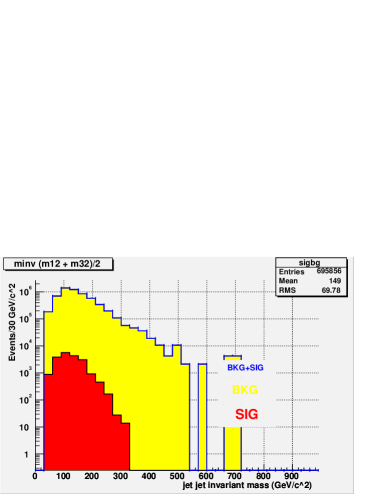
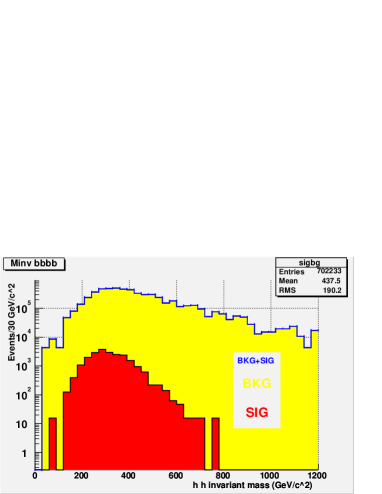
Figure 4: Reconstructed di-jet (left) and four-jet mass (right) for signal and background.

3 CONCLUSION

We estimated the CMS discovery potential for the radion into two Higgs decay mode ($\phi\rightarrow\rm h\rm h$) with $\gamma\gamma$+$\rm b\bar{\rm b}$, $\tau\tau$+$\rm b\bar{\rm b}$ and $\rm b\bar{\rm b}$+$\rm b\bar{\rm b}$ final states. One point of $\rm m_{\phi}$=300 GeV/$c^{2}$ and $\rm m_{\rm h}$=125 GeV/$c^{2}$ was taken and the observability in the ($\xi$, $\Lambda_{\phi}$) plane was evaluated. It was found that the $\gamma\gamma$+$\rm b\bar{\rm b}$ topology provides the best discovery potential. The $\rm b\bar{\rm b}$+$\rm b\bar{\rm b}$ final state requires the dedicated High Level Trigger with the double b tagging and an excellent understanding of the background shape.

ACKNOWLEDGEMENTS

A.N. would like to thank M. Dubinin for CompHEP generation of $\gamma\gamma\rm j\rm j$ events and F. Maltoni for explanations about the MadGraph generator.

Part XVI The Invisible Higgs Decay Width In The ADD Model At The LHC

M. Battaglia, D. Dominici, J.F. Gunion and J.D. Wells

1 INTRODUCTION

In several extensions of the Standard Model (SM) there exist mechanisms that modify the Higgs production/decay rates in channels that are observable at the LHC. One example is the Randall Sundrum model where the Higgs-radion mixing not only gives detectable reductions (or enhancements) in Higgs yields, but also allows the possibility of direct observation of radion production and decay [139, 147]. It is also possible for the Higgs rate in visible channels to be reduced as a result of a substantial invisible width. For example, this occurs in supersymmetric models when the Higgs has a large branching ratio into the lightest gravitinos or neutralinos. Invisible decay of the Higgs is also predicted in models with large extra dimensions felt by gravity (ADD) [159, 160]. In ADD models the presence of an interaction between the Higgs $H$ and the Ricci scalar curvature of the induced 4-dimensional metric $g_{\rm ind}$, generates, after the usual shift $H=({v+h\over\sqrt{2}},0)$, the following mixing term [136]

$${\cal L}_{\rm mix}=\epsilon h\sum_{\vec{n}>0}s_{\vec{n}}$$ (1)

with

$$\epsilon=-{2\sqrt{2}\over M_{P}}\xi vm_{h}^{2}\sqrt{{3(\delta-1)\over\delta+2}}\,.$$ (2)

Above, $M_{P}=(8\pi G_{N})^{-1/2}$ is the Planck mass, $\delta$ is the number of extra dimensions, $\xi$ is a dimensionless parameter and $s_{\vec{n}}$ is a graviscalar KK excitation with mass $m_{\vec{n}}^{2}=4\pi^{2}\vec{n}^{2}/L^{2}$, $L$ being the size of each of the extra dimensions. (Note that with respect to [136] our normalization is such that we have taken only the real part of the $\phi_{G}^{\vec{n}}$ fields, writing $\phi_{G}^{\vec{n}}={1\over\sqrt{2}}(s_{\vec{n}}+ia_{\vec{n}})$ and using $\phi_{G}^{\vec{n}}=[\phi_{G}^{-\vec{n}}]^{*}$ to restrict sums to $\vec{n}>0$, by which we mean that the first non-zero entry of $\vec{n}$ is positive.) After diagonalization of the full mass-squared matrix one finds that the physical eigenstate, $h^{\prime}$, acquires admixtures of the graviscalar states and vice versa. Dropping ${\cal O}(\epsilon^{2})$ terms and higher,

$$h^{\prime}\sim\left[h-\sum_{\vec{m}>0}{\epsilon\over m_{h}^{2}-im_{h}\Gamma_{h}-m_{\vec{m}}^{2}}s_{\vec{m}}\right]\,,\quad s^{\prime}_{\vec{m}}\sim\left[s_{\vec{m}}+{\epsilon\over m_{h}^{2}-im_{h}\Gamma_{h}-m_{\vec{m}}^{2}}h\right]\,.$$ (3)

In computing a process such as $WW\rightarrow h^{\prime}+\sum_{\vec{m}>0}s_{\vec{m}}^{\prime}\rightarrow F$, normalization and admixture corrections of order $\epsilon^{2}$ that are present must be taken into account and the full coherent sum over physical states must be performed. The result at the amplitude level is

$${\cal A}(WW\rightarrow F)(p^{2})\sim{g_{WWh}g_{hF}\over p^{2}-m_{h}^{2}+im_{h}\Gamma_{h}+iG(p^{2})+F(p^{2})}$$ (4)

where $F(p^{2})\equiv-\epsilon^{2}{\rm Re}\left[\sum_{\vec{m}>0}{1\over p^{2}-m_{\vec{m}}^{2}}\right]$ and $G(p^{2})\equiv-\epsilon^{2}{\rm Im}\left[\sum_{\vec{m}>0}{1\over p^{2}-m_{\vec{m}}^{2}}\right]$. Taking the amplitude squared and integrating over $dp^{2}$ in the narrow width approximation gives the result

$$\sigma(WW\rightarrow h^{\prime}+\sum_{\vec{m}>0}s^{\prime}_{\vec{m}}\rightarrow F)=\sigma_{SM}(WW\rightarrow h\rightarrow F)\left[{1\over 1+F^{\prime}(m_{h\,{\rm ren}}^{2})}\right]\left[{\Gamma_{h}\over\Gamma_{h}+\Gamma_{h\rightarrow{\rm graviscalar}}}\right]$$ (5)

where $m_{h\,{\rm ren}}^{2}-m_{h}^{2}+F(m_{h\,{\rm ren}}^{2})=0$ and we have defined $m_{h}\Gamma_{h\rightarrow{\rm graviscalar}}\equiv G(m_{h\,{\rm ren}}^{2})$. We will argue that for a light Higgs boson both the wave function renormalization and the mass renormalization effects will be small. In this case, the coherently summed amplitude gives the Standard Model cross section suppressed by the ratio of the SM Higgs width to the sum of the SM Higgs width and the Higgs width arising from mixing with the graviscalars.

2 INVISIBLE WIDTH

As described, there is a decay of the Higgs arising from the mixing (or oscillation) of the Higgs itself into the closest KK graviscalar levels. These graviscalars are invisible since they are weakly interacting and mainly reside in the extra dimensions whereas the Higgs resides on the brane. The mixing width $\Gamma_{h\rightarrow{\rm graviscalar}}\sim G(m_{h}^{2})/m_{h}$ thus corresponds to an invisible decay width. The equation for $G(m_{h}^{2})$ below eq. (4) shows that it is calculated by extracting the imaginary part of the mixing contribution to the Higgs self energy. The result is [136, 161]

$$\Gamma(h\rightarrow{\rm graviscalar}) \equiv \Gamma(h\rightarrow\sum_{\vec{n}>0}s_{\vec{n}})=2\pi\xi^{2}v^{2}\frac{3(\delta-1)}{\delta+2}\frac{m_{h}^{1+\delta}}{M_{D}^{2+\delta}}{S_{\delta-1}}$$ (6)

$$\sim (16\,\leavevmode\nobreak\ {\rm MeV})20^{\delta-2}\xi^{2}S_{\delta-1}\frac{3(\delta-1)}{\delta+2}\left(\frac{m_{h}}{150\,\leavevmode\nobreak\ {\rm GeV}}\right)^{1+\delta}\left(\frac{3\,{\rm TeV}}{M_{D}}\right)^{2+\delta}$$

where $S_{\delta-1}=2\pi^{\delta/2}/\Gamma(\delta/2)$ denotes the surface of a unit radius sphere in $\delta$ dimensions while $M_{D}$ is related to the $D$ dimensional reduced Planck constant ${\overline{M}}_{D}$ by $M_{D}=(2\pi)^{\delta/(2+\delta)}{\overline{M}}_{D}$. Our eqs. (6) are a factor of 2 larger than those presented in refs. [136, 161].

2.1 The wave function renormalization factor and mass renormalization

A simple estimate of the quantity $F^{\prime}(m_{h\,{\rm ren}}^{2})$, appearing in the wave function renormalization factor found in eq. (5), suggests that it is of order $\xi^{2}{m_{h}^{4}\over\Lambda^{4}}$, where $\Lambda$ is an unknown ultraviolet cutoff energy presumably of order $\Lambda\sim M_{D}$ [162]. Assuming this to be the case, $F^{\prime}$ will provide a correction to coherently computed LHC production cross sections that is very probably quite small for the $m_{h}\ll M_{D}$ cases that we are about to explore. However, one must keep in mind that a precise calculation of $F^{\prime}$ is not possible. Similarly, the mass renormalization from $F(m_{h\,{\rm ren}}^{2})$ should be of order $\xi^{2}m_{h}^{6}/M_{D}^{4}$ and, therefore, small for $m_{h}\ll M_{D}$. There are other incomputable sources of $v^{4}/M_{D}^{4}$ corrections lurking in the theory beyond these sources, and the results presented here are computed using the first, and perhaps only, calculable terms in the perturbation series.

2.2 Contribution to the invisible width from direct two graviscalar decay

In addition to decay by mixing, one expects also a contribution to the invisible width of the Higgs from its decays into two graviscalars. This can be evaluated by using the transformation of eq. (3) between the physical eigenstate $h^{\prime}$ and the unmixed $h$ to derive the relevant trilinear $h^{\prime}s_{k}s_{l}$ vertices. These are used to compute the corresponding matrix element. The final expression for $\Gamma(h^{\prime}\rightarrow{\rm graviscalar\leavevmode\nobreak\ pairs})$ can be written as

$$\Gamma(h^{\prime}\rightarrow{\rm graviscalar\leavevmode\nobreak\ pairs}) = {18\over\pi}{m_{h}^{3+2\delta}v^{2}\over M_{D}^{4+2\delta}}\xi^{4}\left({\delta-1\over\delta+2}\right)^{2}\left[{\pi^{\delta/2}\over\Gamma(\delta/2)}\right]^{2}I\,,$$ (7)

where $I$ is an integral coming from the sum over all the possible kinematically allowed $h^{\prime}\rightarrow s_{k}s_{l}$ decays. The integral $I$ decreases rapidly as $\delta$ increases. As a result, $\Gamma(h^{\prime}\rightarrow{\rm graviscalar\leavevmode\nobreak\ pairs})$ is only significant compared with $\Gamma(h\rightarrow{\rm graviscalar})$ if $\delta\leq 4$. The ratio of the two widths is given by:

$${\Gamma(h^{\prime}\rightarrow{\rm graviscalar\leavevmode\nobreak\ pairs})\over\Gamma(h\rightarrow{\rm graviscalar})}={3(\delta-1)\over 2\pi^{2}(\delta+2)}\xi^{2}\left({m_{h}\over M_{D}}\right)^{2+\delta}{\pi^{\delta/2}\over\Gamma(\delta/2)}I\,.$$ (8)

From this result, we immediately see that even for small $\delta$ the pair invisible width will be smaller than the mixing invisible width unless $m_{h}$ is comparable to $M_{D}$.

To lowest order in $\xi^{2}(m_{h}/M_{D})^{2+\delta}$, decays of other states nearly degenerate with the $h^{\prime}$ can be neglected in the computation of a cross section obtained by coherently summing over the $h^{\prime}$ and the nearly degenerate $s^{\prime}_{\vec{m}}$ states. Thus, to this same order of approximation, $\Gamma(h^{\prime}\rightarrow{\rm graviscalar\leavevmode\nobreak\ pairs})$ should simply be added to $\Gamma(h\rightarrow{\rm graviscalar})$ in the expression for the narrow-width cross section of eq. (5).

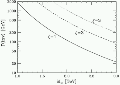
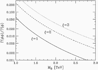
Figure 1: In the left-hand plot, we display the total invisible width of a 1 TeV Higgs boson into one and two graviscalars as a function of $M_{D}$ for various values of $\xi$ ($\xi=1$ solid, $\xi=2$ dashed, $\xi=3$ dotted). For these plots we have fixed $\delta=2$. The plot on the right shows the ratio of the two-graviscalars decay width to the one-graviscalar decay width for the same choices of parameters.

In Figure 1, we show an extreme case corresponding to $\delta=2$ and $m_{h}=1000\leavevmode\nobreak\ {\rm GeV}$. Depending on the values of the parameters $\xi$ and $M_{D}$, the pair invisible width can be a significant correction to the invisible width from direct mixing. More generally, for $m_{h}>M_{D}$ the graviscalar-pair invisible width can provide a 3% to 20% correction to the direct-graviscalar-mixing invisible width. However, if $m_{h}$ is substantially smaller than $M_{D}$, then the graviscalar pair width is not important. For example, for $\delta=2$, $m_{h}=120\leavevmode\nobreak\ {\rm GeV}$ and $M_{D}=500\leavevmode\nobreak\ {\rm GeV}$, $\Gamma(h^{\prime}\rightarrow{\rm graviscalar\leavevmode\nobreak\ pairs})/\Gamma(h\rightarrow{\rm graviscalar})<0.0015$ for $\xi<2$. Therefore, in the following analysis, where we will assume a light Higgs, we can safely neglect the contribution to the invisible width from the decay into two graviscalars and use the expression given by eq. (6).

3 MEASUREMENTS AT THE LHC

For a Higgs boson with $m_{h}$ below the $WW$ threshold, the invisible width causes a significant suppression of the LHC Higgs rate in the standard visible channels. For example, for $\delta=2$, $M_{D}=500\leavevmode\nobreak\ {\rm GeV}$ and $m_{h}=120\leavevmode\nobreak\ {\rm GeV}$, $\Gamma(h\rightarrow{\rm graviscalar})$ is of order $50\leavevmode\nobreak\ {\rm GeV}$ already by $\xi\sim 1$, i.e. far larger than the SM prediction of $3.6\leavevmode\nobreak\ {\rm MeV}$. Even when $m_{h}$ is greater than the $WW$ threshold, Figure 1 shows that the partial width into invisible states can be substantial even for $M_{D}$ values of several TeV; therefore, for any given value of the Higgs boson mass, there is a considerable parameter space where the invisible decay width of the Higgs boson could be the first measured phenomenological effect from extra dimensions.

Detailed studies of the Higgs boson signal significance, with inclusive production, have been carried out by the ATLAS [79] and CMS  [163] experiments. If 115 GeV $<m_{h}<$ 130 GeV, the $h\rightarrow\gamma\gamma$ channel appears to be instrumental for obtaining a $\geq 5\sigma$ signal at low luminosity. The $t\bar{t}h$, $h\rightarrow b\bar{b}$ and $h\rightarrow ZZ^{*}\rightarrow 4\leavevmode\nobreak\ \ell$ channels also contribute, with lower statistics but a more favorable signal-to-background ratio. Preliminary results indicate that Higgs boson production in association with forward jets may also be considered as a discovery mode. However, here the background reduction strongly relies on the detailed detector response.

In the ADD model, these results are modified by the appearance of an invisible decay width suppressing the Higgs signal in the standard visible channels. Here, we fix $m_{h}=120\leavevmode\nobreak\ {\rm GeV}$ and perform a full scan of the ADD parameter space by varying $M_{D}$ and $\xi$ for different values of the number of extra dimensions $\delta$ and demonstrate that there are regions at high $\xi$ where the significance of the Higgs boson signal in the canonical channels drops below the 5 $\sigma$ threshold. However, the LHC experiments will also be sensitive to an invisibly decaying Higgs boson through $WW$-fusion production, with tagged forward jets. A detailed CMS study has shown that, with only 10 fb^-1, an invisible channel rate of $\Gamma_{\rm inv}/\Gamma$=0.12-0.20 times the SM $WW\rightarrow$Higgs production rate gives a signal exceeding the 95% CL significance for 120 GeV $<m_{h}<$ 400 GeV [164, 163]. Given that the effective (from the sum over the $h$ state and nearby degenerate states) $WWh$ coupling is of SM strength, this defines the region in the ADD parameter space where the Higgs boson signal can be recovered through its invisible decay .

Figure  2 summarizes the results for specific choices of parameters. In the green (light grey) region, the Higgs signal in standard channels drops below the 5 $\sigma$ threshold with 30 fb^-1 of LHC data. But in the area above the bold blue line the LHC search for invisible decays in the fusion channel yields a signal with an estimated significance exceeding 5 $\sigma$. It is important to observe that, whenever the Higgs boson sensitivity is lost due to the suppression of the canonical decay modes, the invisible rate is large enough to still ensure detection through a dedicated analysis.

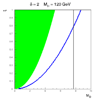
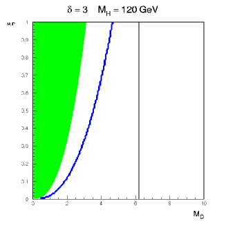
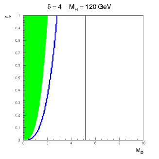
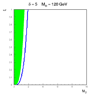
Figure 2: Invisible decay width effects in the $\xi$ - $M_{D}$ plane for $M_{H}$ = 120 GeV. The green (grey) regions indicate where the Higgs signal at the LHC drops below the 5 $\sigma$ threshold for 30 fb^-1 of data. The regions above the blue (bold) line are the parts of the parameter space where the invisible Higgs signal in the $WW$-fusion channel exceeds 5 $\sigma$ significance. The vertical lines show the upper limit on $M_{D}$ which can be probed by the analysis of jets/$\gamma$ with missing energy at the LHC. The plots are for different values of $\delta$: 2 (upper left), 3 (upper right), 4 (lower left), 5 (lower right).

The analysis of jet/$\gamma+$ missing energy is also sensitive to the ADD model over a range of the $M_{D}$ and $\delta$ parameters [165]. The invisible Higgs decay width appears to probe a parameter space up to, and possibly beyond, that accessible to these signatures (see Figure 2). Further, the sensitivity of these channels decreases significantly faster with $\delta$ than that of the invisible Higgs width if $\xi\sim 1$. Finally, it is interesting that, in the region where both signatures can be probed at the LHC, a combined analysis will provide a constraint on the fundamental theory parameters. A TeV-class $e^{+}e^{-}$ linear collider will be able to further improve the determination of the Higgs invisible width. Extracting the branching fraction into invisible final states from the Higgsstrahlung cross section and the sum of visible decay modes affords an accuracy of order 0.2-0.03% for values of the invisible branching fraction in the range 0.1-0.5. But the ultimate accuracy can be obtained with a dedicated analysis looking for an invisible system recoiling against a $Z$ boson in the $e^{+}e^{-}\rightarrow hZ$ process. A dedicated analysis has shown that an accuracy $0.025<\delta{\mathrm{BR}}/{\mathrm{BR}}<0.04$ can be obtained for $0.1<{\mathrm{BR}}<0.5$ [166]. This accuracy would establish an independent constraint on the $M_{D}$, $\xi$ and $\delta$ parameters.

ACKNOWLEDGEMENTS

JFG and JDW are supported by the U.S. Department of Energy.

Part XVII Determining the extra-dimensional location of the Higgs boson

A. Aranda, C. Balázs, J. L. Díaz-Cruz S. Gascon-Shotkin and O. Ravat

1 INTRODUCTION

Extra dimensional models have been used recently to address a wide class of problems in particle physics, such as the hierarchy, unification and flavor problems [159, 160, 167, 168]. In this work, we examine a TeV^-1 size extra dimensional model, in which the lightest Higgs boson emerges as an admixture of brane and bulk scalar fields. This model predicts a suppression of the Higgs production cross section at LEP and the Tevatron, while it promises a significant enhancement of the signal at the CERN Large Hadron Collider (LHC) and possibly at a multi TeV linear collider (CLIC). We present results for the cross section of the associated production of Higgs with gauge bosons at the LC and LHC.

2 THE MODEL

In this section we present the general features of the extra dimensional model (for a detailed description see [169]). We work with a five dimensional (5D) extension of the SM that contains two Higgs doublets. The SM fermions and one Higgs doublet ($\Phi_{u}$) live on a 4D boundary, the brane, while the gauge bosons and the second Higgs doublet ($\Phi_{d}$), are all allowed to propagate in the bulk. The constraints from electroweak precision data [168] show that the compactification scale can be of ${\cal O}$(TeV) (3-4 TeV at 95 % C.L.). The relevant terms of the 5D $SU(2)\times U(1)$ gauge and Higgs Lagrangian are given by

$${\cal L}^{5}=-\frac{1}{4}\left(F^{a}_{MN}\right)^{2}-\frac{1}{4}\left(B_{MN}\right)^{2}+|D_{M}\Phi_{d}|^{2}+|D_{\mu}\Phi_{u}|^{2}\delta(x^{5})\,,$$ (1)

where the Lorentz indices $M$ and $N$ run from $0$ to $4$, and $\mu$ runs from $0$ to $3$.

After spontaneous breaking of electroweak symmetry one obtains the following 4D Lagrangian:

$${\cal L}^{4} \supset \frac{gM_{Z}}{2c_{W}}\left(h\sin(\beta-\alpha)+H\cos(\beta-\alpha)\right)Z_{\mu}Z^{\mu}$$ (2)

$$+ \sqrt{2}\frac{gM_{Z}}{c_{W}}\left(h\sin\beta\cos\alpha+H\sin\beta\sin\alpha\right)\sum_{n=1}^{\infty}Z_{\mu}^{(n)}Z^{\mu}$$

$$+ gM_{W}\left(h\sin(\beta-\alpha)+H\cos(\beta-\alpha)\right)W^{+}_{\mu}W^{-\mu}$$

$$+ \sqrt{2}gM_{W}\left(h\sin\beta\cos\alpha+H\sin\beta\sin\alpha\right)\sum_{n=1}^{\infty}\left(W^{+}_{\mu}W^{-(n)\mu}+W^{-}_{\mu}W^{+(n)\mu}\right)\,.$$

where $h$ and $H$ are the CP-even Higgses ($m_{h}<m_{H}$), $\alpha$ is the mixing angle that appears in the diagonalization of the CP-even mass matrix, and $\tan\beta$ is the ratio of vevs.

3 HIGGS PRODUCTION AT FUTURE COLLIDERS

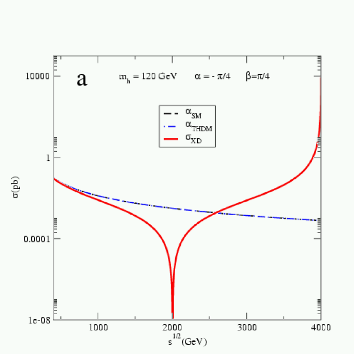
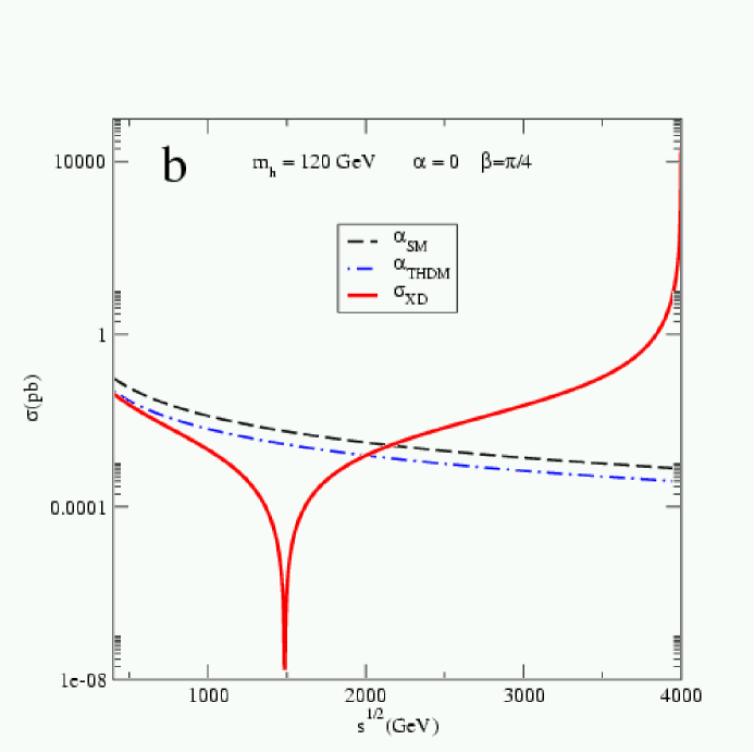
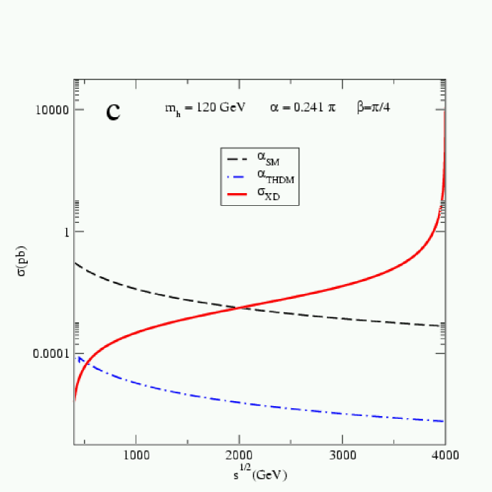
Figure 1: SM, THDM and XD cross sections for $e^{+}e^{-}\rightarrow Zh$. Each plot corresponds to a different set of values for $\alpha$ and $\beta$ all with $m_{h}=120$ GeV and with a compactification scale $M_{c}=4$ TeV.

We present results for the associated $h+Z$ production cross section obtained from Eq.(2) at linear colliders and at the LHC. Fig. 1 shows the results for the $e^{+}e^{-}\rightarrow hZ$ cross section. $\sigma_{SM}$ stands for the standard model cross section, THDM labels the (4D) two Higgs doublet model, and the results from the extra dimensional model are denoted by XD. The three plots correspond to three different choices of the parameters $\alpha$ and $\beta$. It can be observed that the SM cross section dominates in all cases up to $\sqrt{s}\sim 2$ TeV. This is understood from the fact that the heavier KK modes, through their propagators, interfere destructively with the SM amplitude thus reducing the XD cross section. Moreover, as Fig. 1 shows, once the center of mass energy approaches the threshold for the production of the first KK state, the cross section starts growing. For instance, with $M_{c}=4$ TeV, $\sigma_{SM}\simeq\sigma_{XD}$ for $\sqrt{s}\simeq 2$ TeV. However, one would need higher energies in order to have a cross section larger than that of the SM, which may only be possible at CLIC [170]. Based on this, we also conclude that at the Tevatron the luminosity required to find a light Higgs boson is higher than in the SM case.

The Higgs discovery potential in this model is more promising at the LHC. We illustrate this in Fig. 2, showing the $pp\rightarrow hZ$ differential cross section as the function of the $hZ$ invariant mass $M_{hZ}$. The typical resonance structure displayed by Fig.1 is preserved by the hadronic cross section. The resonance peak is well pronounced when $M_{hZ}\sim M_{c}$. This leads to a large enhancement over the SM (or THDM) cross section. The singularity at $M_{c}=M_{hZ}$ is regulated by the width of the KK mode, which is included in our calculation (cf. Ref.[169]). Depending on the particular values of $\alpha$ and $\beta$ the enhancement is more or less pronounced. For an optimistic set $\alpha=0$ and $\beta=\pi/2$, the XD production cross section is considerably enhanced compared to the SM at $M_{hZ}=M_{c}$. This enhancement may be detectable up to about $M_{c}=6$ TeV. We estimate that with 100 fb^-1 for $M_{c}=6$ TeV there are about 20 $hZ$ events in the bins around $M_{hZ}\sim M_{c}$. As Fig. 2 shows, in the SM less than one event is expected in the same $M_{hZ}$ range. It is needless to say that similar results hold for $pp\rightarrow hW^{\pm}$, which further enhances the discovery prospects.

Based on these results, we conclude that in the Bjorken process alone the reach of the LHC may extend to about $M_{c}=6$ TeV, depending on the values of $\alpha$ and $\beta$. The $Zh$ (or $W^{\pm}h$) production cross section determines only a specific combination of the mixing angles $\alpha$ and $\beta$. In order to determine the individual angles, one has to also measure the production cross sections of the heavier Higgs boson in association with a $Z$ (or $W^{\pm}$). Fortunately, these cross sections are also enganced by the same amount as the ones for the lightest Higgs boson.

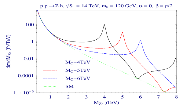
Figure 2: Higgs production cross section in association with a $Z$ boson at the LHC as a function of the compactification scale for selected values of the mixing parameters.

4 CONCLUSIONS

We presented Higgs production cross section calculations in the framework of an extra dimensional model that releaves the tension between the low mass predictions for the SM Higgs and the missing Higgs signal at LEP. We found a suppresson at the LC and at the Tevatron, but an enhanced signal at the LHC or CLIC. The fact that the lightest Higgs boson is an admixture of brane and bulk fields (that is it has a non-trivial bulk location) is the key ingredient in the suppression-enhancement mechanism for the signal. This may enable the LHC and CLIC to determine this location.

ACKNOWLEDGEMENTS

A.A. acknowledges support from the Alvarez-Buylla fund of the Universidad de Colima. During this work, CB was supported by the U.S. Department of Energy HEP Division under contracts DE-FG02-97ER41022 and W-31-109-ENG-38, and by LPNHE-Paris. J.L. D.-C. was supported by CONACYT and SNI (México).

Part XVIII The sensitivity of the LHC for TeV scale dimensions in dijet production

C. Balázs, M. Escalier, S. Ferrag, B. Laforge and G. Polesello

1 Introduction

String theory is the most promising candidate for a unified framework of matter and interactions. Among the predictions of string theory are extra, compact space dimensions (XDs) which, depending on their sizes $R$, play a role in determining physics close to the weak scale. The string arguments of Refs. [171, 172] do not prevent the standard gauge bosons from penetrating the bulk. If the compactification scale $M_{c}=1/R$ is higher than ${\cal O}$(TeV), phenomenology and present experiments do not conflict with this scenario either [173, 174, 175, 176, 167, 177]. These new dimensions, on the other hand, may be probed at near future particle accelerators, in particular at the CERN Large Hadron Collider (LHC).

Since the LHC produces strongly interacting particles abundantly, if the gluons propagate in XDs then dijet production at the LHC is a sensitive discovery channel for TeV scale XDs. The main effect of these dimensions on the dijet production cross section is twofold. On the one hand, the gluonic Kaluza-Klein (KK) excitations enhance the dijet distributions in the high invariant mass (${\hat{s}}$) and transverse momentum ($p_{T}$) region [178]. On the other, the modified evolution of the strong coupling ($\alpha_{S}$) further distorts these distributions [179]. These competing effects are entangled and has to be taken into account simultaneously in order to predict the discovery potential of the LHC.

In this work, we computed dijet distributions for the LHC including both of these effects. We assumed that the standard model (SM) gauge bosons, especially gluons, propagate in a single TeV^-1 size compact dimension. We implemented gluonic KK excitations and the modified running of $\alpha_{S}$ in the Monte Carlo event generator PYTHIA [15], for dijets. Then, we used PYTHIA to calculate dijet $p_{T}$ distributions, determined the enhancement at large $p_{T}$, and estimated the significance of a potential discovery.

2 Dijet production at the LHC

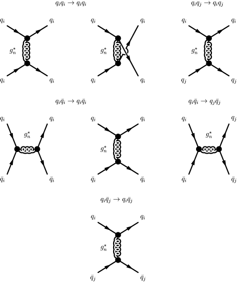
Figure 1: Feynman diagrams for dijet production involving Kaluza-Klein excitations of the gluons. The indices $i$ and $j$ represent distinct ($i\neq j$) quark flavors.

The formalism that we use is described in detail in Refs.[178] and [179]. When calculating the dijet production cross section, besides the SM ones, we include the tree-level diagrams shown in Fig. 1. In these diagrams $g_{n}^{*}$ signals that a KK tower of virtual gluons is exchanged. This means that in the SM diagrams we replace the gluon propagators by

$$D_{\mathit{eff}}(p)=\sum_{n=0}^{N}c_{n}D_{n}(p).$$ (1)

Here

$$D_{n}(p)=\frac{c_{n}}{p_{n}^{\prime 2}+im_{n}\Gamma_{n}},$$ (2)

is the propagator of the $n^{th}$ gluon KK resonance with $p_{n}^{\prime 2}=p^{2}-m_{n}^{2}$, $c_{n>0}=2$, $m_{n}=n/R,\Gamma_{n}=2\alpha_{s}m_{n}$. The SM gluon is identified with the zero mode and $c_{0}=1$.

When calculating the cross section, it is necessary to evaluate amplitude squares which will contain products of propagators of the form

$$\frac{1}{2}\mbox{\raisebox{-2.58334pt}{\huge$[$}}D_{\mathit{eff}}^{\star}(p)D_{\mathit{eff}}(q)+D_{\mathit{eff}}(p)D_{\mathit{eff}}^{\star}(q)\mbox{\raisebox{-2.58334pt}{\huge$]$}}=$$

$$\sum_{m,n=0}^{N}\frac{c_{m}c_{n}(p_{m}^{\prime 2}q_{n}^{\prime 2}+m_{m}\Gamma_{m}m_{n}\Gamma_{n})}{((p_{m}^{\prime 2})^{2}+m_{m}^{2}\Gamma_{m}^{2})((q_{n}^{\prime 2})^{2}+m_{n}^{2}\Gamma_{n}^{2})}\,$$ (3)

(We note that in Eq.(3), we corrected a typo which is present in v.3 of hep-ph/0012259.) As it was noted in Ref. [178] the sum in Eq. (3) converges rapidly. We checked that for the LHC (with $\sqrt{(S)}=14$ TeV) and for $M_{c}>1$ TeV, choosing $N=50$ (or equivalently a cutoff scale of $M_{s}>50$ TeV) leads to a satisfactory numerical precision. We implemented the effective propagators given by Eq.(3) in PYTHIA, modifying the parton level processes represented by Fig.(1). Finally, we checked the implementation against the numerical results given in Ref. [178] and found a good agreement.

In our calculation, we also include the modified running of $\alpha_{S}$, as described in Refs.[167, 177, 179]. Above the compactification scale, we implemented the modified running of $\alpha_{s}$ as given by

$$\alpha_{i}^{-1}(\mu)=\alpha_{i}^{-1}(\mu_{0})-{b_{i}-\tilde{b}_{i}\over 2\pi}\,\ell_{\rm n}{\mu\over\mu_{0}}-\leavevmode\nobreak\ {\tilde{b}_{i}\over 4\pi}\,\int_{r\mu^{-2}}^{r\mu_{0}^{-2}}{dt\over t}\,\left[\vartheta_{3}\left({it\over\pi R^{2}}\right)\right]^{\delta},$$ (4)

where $i=1,2,3$ labels the gauge groups of the SM. The coefficients of the usual one loop beta functions

$$(b_{1},b_{2},b_{3})=(41/10,-19/6,-7)$$ (5)

are supplemented by new contributions from the KK towers

$$(\tilde{b}_{1},\tilde{b}_{2},\tilde{b}_{3})=(3/5,-3,-6)+\eta\;(4,4,4)$$ (6)

(where, for simplicity, we set $\eta=0$). In the last term of Eq. (4), $\vartheta_{3}$ denotes the elliptic Jacobi function and

$$r=\pi\,(X_{\delta})^{-2/\delta}\leavevmode\nobreak\ \leavevmode\nobreak\ \leavevmode\nobreak\ {\rm with}\leavevmode\nobreak\ \leavevmode\nobreak\ \leavevmode\nobreak\ X_{\delta}={2\pi^{\delta/2}\over\delta\Gamma(\delta/2)}.$$ (7)

We note that in Refs. [167, 177] an approximate expression is used to calculate the running of the couplings, but we implemented the exact formula (4) in PYTHIA.

3 Numerical results

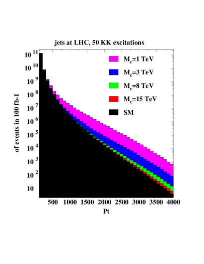
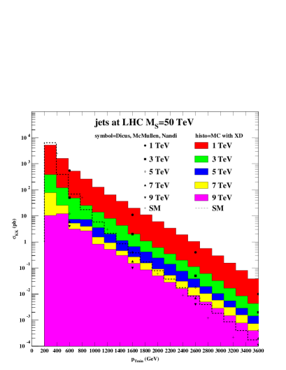
Figure 2: Left panel: number of dijet events vs. the dijet $p_{T}$ calculated in the SM and for various values of $M_{c}$. Right panel: KK contribution to the cross section as the function of $p_{T{\rm min}}$.

Our goal is to quantify the sensitivity of the LHC to a TeV size XD. To this end, following Ref. [178], we compute the dijet transverse momentum ($p_{T}$) distribution. As a first step, we include 50 KK excitations of the gluons but keep the standard evolution of $\alpha_{s}$. We use PYTHIA version 6.210 with the modifications described in the previous section. On the final state, we apply the following kinematic cuts:

$$p_{T}>p_{T{\rm min}},\leavevmode\nobreak\ \leavevmode\nobreak\ \leavevmode\nobreak\ |y|<2.5,\leavevmode\nobreak\ \leavevmode\nobreak\ \leavevmode\nobreak\ p_{Tjet}>100\leavevmode\nobreak\ {\rm GeV\leavevmode\nobreak\ (on\leavevmode\nobreak\ each\leavevmode\nobreak\ jet)},$$ (8)

where $y$ is the rapidity of the two jet system. In PYTHIA, we also turn the initial and final state radiation (ISR and FSR) on.

The left panel of Fig. 2 shows the results as the number of dijet events against the dijet $p_{T}$ assuming 100 fb^-1 integrated luminosity. In this and in the subsequent computations we used the CTEQ6L1 parton distribution function (PDF) with the dijet invariant mass as the factorization scale. It is shown that there is a significant enhancement in the high $p_{T}$ for $M_{c}=8$ TeV, and there is still a detectable excess for $M_{c}=15$ TeV. The right panel of Fig. 2 shows the KK contribution to the cross section

$$\sigma_{\rm KK}=\sigma_{\rm total}-\sigma_{\rm SM},$$ (9)

as the function of $p_{T{\rm min}}$. Considering the difference in the PDF, slightly different cuts and the PYTHIA effects (ISR, FSR, etc.), our results still reasonably agree with Fig.3 of Ref. [178].

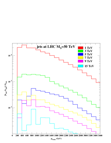
Figure 3: Statistical significance of the XD dijet signal in units of $\sigma$.

Finally, Fig. 3 shows the statistical significance

$$S=|N_{SM}-N_{XD}|/\sqrt{N_{SM}},$$ (10)

of the XD dijet signal in units of $\sigma$ plotted against the dijet $p_{T}$. Here $N_{X}$ is the number of events predicted by model $X$. This plots shows that by measuring the dijet $p_{T}$ distribution in the 1-3 TeV region the new dimension can be easily discovered even if it is as small as 15 TeV^-1.

Acknowledgments

The authors are grateful to the organizers of Les Houches 2003. During this work, CB was supported by the U.S. Department of Energy HEP Division under contracts DE-FG02-97ER41022 and W-31-109-ENG-38, and by Universites Paris VI & VII.

Part XIX Little Higgs Model: LHC Potential

K.Mazumdar

1 INTRODUCTION

The Little Higgs model is an alternative solution for the hierarchy problem in the Standard Model (SM) of strong and electroweak interactions which has passed stringent experimental verifications upto the electroweak scale. The precision measurements indicate that the physical mass of the Higgs boson $m_{\rm H}\leq 219$ GeV/c² to 95% CL. Considering the SM as an effective theory valid upto an energy scale $\sim$ few TeV, any new physics appearing below a cutoff of about 10 TeV has to be weakly coupled to be consistent with precision measurements. The gap between electroweak scale and this cutoff value is called the ’little hierarchy’.

This hierarchy problem is solved in Little Higgs model by requiring $m_{\rm H}$ to be safe from only one-loop divergences. The Higgs fields are considered as Nambu-Goldstone-Bosons of a global symmetry which is spontaneously broken at a higher scale, but the physical Higgs boson states continue to remain light due to approximate global symmetry. In the minimal scenario both gauge and Yukawa interactions are necessary to break all the global symmetry which protect the Higgs boson mass and hence pushes the cutoff scale to $\sim$ 10 TeV. The additional particles postulated in the model are three heavy gauge bosons, a heavy top-like quark (T), a heavy Higgs triplet and a Higgs doublet. The lightest neutral scalar is identified with the SM Higgs boson. Interestingly, the most important divergences are cancelled between loops of particles with the same statistics.

The masses of the new particles need to be light enough to avoid fine tuning, whereas the precision electroweak constraints push them higher. Hence parameters of the model, eg. couplings, need to be tuned. Present expectations of 1-2 TeV mass range make these particles accessible at LHC and this motivates us to study their prospect of discovery.

2 COLLIDER PHENOMENOLOGY

The collider phenomenology has been worked out in  [180]. The heavy gauge bosons can be produced in LHC via Drell-Yan type process. The heavy quark T can be produced via QCD (gluon-gluon fusion) in a model independent way but with increasing mass the cross-section falls off rapidly. It can also be produced singly, through t-channel fusion process $W^{+}b\rightarrow T$, and the cross-section, though larger, depends on the parameters in the model, relating the Top mass $M_{T}$ to the scale, or equivalently to the Higgs condensate $f$ ($\sim$ TeV).

The tree-level Feynman diagram for the production of single T and the cross-section at LHC as a function of its mass is given in Fig. 1. The single T production cross-section is taken as 0.25 pb for $M_{T}=1$ TeV/c².

3 HEAVY TOP SEARCH IN CMS

Figure 1: The tree-level Feynman diagram for the production of single T and the cross-section at LHC as a function of its mass.

We have investigated the potential of CMS experiment at LHC to discover some of these new particles predicted in the model. We report in the following on detection capability and possible discovery of singly-produced T decaying through channels $T\rightarrow th$ and $T\rightarrow tZ$, each with a branching fraction of 25%, where $t,\leavevmode\nobreak\ h,\leavevmode\nobreak\ Z$ are the top quark, the Higgs scalar and the neutral vector boson in SM. The other mode $T\rightarrow bW$, though have 50% branching ratio, is expected to be overwhelmed at LHC by backgrounds and hence we have not studied it.

3.1 Simulation method

We have used Pythia subprocess no. 83 for $4^{th}$ generation heavy quark production in t-channel process $q_{i}f_{j}\rightarrow Q_{k}f_{l}$ ($Q_{k}=T$). Pythia decay table is also modified according to model predictions. Background events are various SM processes and they are generated using Pythia or Alpgen (multi-parton final states) generator. In all cases, CTEQ5L structure function is used.

The detector response is emulated according to CMS experimental characteristics and using a fast monte carlo package CMSJET where detector effects are parametrised using full detector simulation. The jet reconstruction and identification is assumed to be possible upto pseudorapidity $|\eta|\leq 4.5$ and above transverse energy $E_{T}\geq 40$ GeV. The b-tagging of jets plays a crucial role and it is effective upto $|\eta|\leq 2.5$ with an efficiency of about 60%. While considering possible bakground events, we note that the signal may be mimicked due to the mis-identification of a light quark jet as a b-jet, though the probability is about 1% only.

We have first done a preliminary study of the kinematics of the signal event at particle level after event generation through Pythia as exemplified in Fig. 2. The source of the initial state b-quark is gluon splitting and being a t-channel process, both the initial state quarks are reasonably forward going. In the final state the particles are highly energetic as expected due to the heavy mass involved; the rapidity distributions of the decay products from T are central and the outgoing light quark, though not central, has $|\eta|\leq 4.5$ for about 87% of the cases. Hence this light jet can be used for tagging the event selection as will be discussed later. Note, since these are preliminary studies our selections do not include any threshold on the missing transverse energy in the event, though it is reasonably high for signal events.

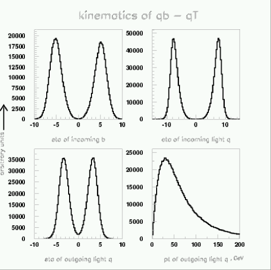
Figure 2: Some of the kinematic distributions of the initial and final state particles in $qb\rightarrow q^{\prime}T$.

4 HEAVY TOP SEARCH IN $T\rightarrow ht,\leavevmode\nobreak\ h\rightarrow b{\bar{b}}$ MODE

In this mode we have investigated the situation where the $W$ from top-quark decays leptonically, i.e., $T\rightarrow ht$, $h\rightarrow b{\bar{b}}$, $t\rightarrow bW,\leavevmode\nobreak\ \leavevmode\nobreak\ W\rightarrow\ell\nu$ where $\ell=e,\leavevmode\nobreak\ \mu$. For a higgs boson mass of 200 GeV/c², the decay branching to $b\bar{b}$ pair is about 65%, so the rate of the final state, given by the signal production cross-section times the relevant branching ratios, is 8.9 fb. The final state contains three b-jets, one isolated lepton, missing transverse energy and one light-jet. For background we have considered the following SM processes:

• $pp\rightarrow t{\bar{t}}$ production with subsequent decays of top-quarks to $bW$ mode. We consider here the leptonic decay of one W and the hadronic decay of the other. We have used Pythia to generate such events and the leading order cross-section is 435 pb.

• $pp\rightarrow Wbbjj$ with a total cross-section of 3.95 pb, including BR($W\rightarrow\ell\nu$).

• $pp\rightarrow W+4jets$ with a total cross-section of 146 pb, including BR($W\rightarrow\ell\nu$).

For processes (2) and (3) we used Alpgen generator and are limited by statistics.

4.1 Possibility of Trigger

To judge the trigger viability of the signal events, we resort to CMS-designed set of criteria for triggering interesting physics events where the threshold values are decided by the DAQ capability. Triggering with an isolated lepton (inclusive) is a suitable condition in this case due to the leptonic decay mode of W. The reconstruction efficiencies for electron and muon events are different and are taken into account to determine the signal selection efficiency according to the following set of kinematic criteria.

• Electron: $p_{T}\geq 29$ GeV/c, $|\eta|\leq 2.5$ with exclusion of $1.442\leq|\eta|\leq 1.566$

• Muon: $p_{T}\geq 14$ GeV/c, $|\eta|\leq 2.1$

• Total selection efficiency for electron and muon events are 0.607 and 0.852 resp.ly. These numbers are also independent of $m_{\rm H}$ in the interesting region.

4.2 Event Selection

We now discuss the main features of signal vis-a-vis the main background of $t\bar{t}$ events after they have passed the detector simulation and the trigger selection criteria. The momentum distribution of the lepton from the signal $T\rightarrow ht\rightarrow$ 3 b-jets + 1 lepton + (light-jet) event is harder compared to that from $t\bar{t}\rightarrow b\bar{b},\leavevmode\nobreak\ W_{1}\rightarrow l\nu,\leavevmode\nobreak\ W_{2}\rightarrow jj$ event. The b-tagged jets are both central and also more energetic. The 4-th jet is typically due to a light quark and is mostly in the higher pseudo-rapidity region as expected for signal events. We have applied the following set of criteria to select signal events; the succesive efficiency factors are also quoted.

• 1 isolated lepton at trigger level, efficiency = 0.73 .

• Total no of jets with transverse energy $E_{T}\geq 60$ GeV in the event = 4, among which three most energetic jets are b-tagged, efficiency = 0.007 .

• First 3 jets should have minimum transverse energy $E_{T}\geq\leavevmode\nobreak\ 200,\leavevmode\nobreak\ 125,\leavevmode\nobreak\ 80$ Gev, $|\eta|\leq 2.3$ and 4th jet should be in the forward/backward region $|\eta|\geq 3.0$, efficiency = 0.29 .

• Transverse momentum of the isolated lepton,  $p_{T}^{\ell}\geq 40$ GeV/c, efficiency = 0.82 .

Combining all we get a grand efficiency of 0.12%, whereas the signal cross-section is 8.9 fb. Hence we conclude that the signal rate is too small to be observed even with large accumulated luminosity.

The above selection criteria could be relaxed and optimised by demanding, for example, less number of b-tagged jets. Evidently with a demand of three b-tagged jets very few events from the background processes could survive due to jet mistagging, but none survived all the selections. This situation may change if we require only one or two b-tagged jets. We should also generate events of type $t\bar{t}$ +jets using Alepgen.

To make our exercise complete, the mass of the higgs boson from the two b-jets with minimal separation, $\Delta R=\sqrt{(}\Delta\eta^{2}+\Delta\phi^{2})$, is reconstructed and subsequently the transverse mass of T also can be reconstructed. This can finally lead to the estimation of the model parameter. We note here that the distance between the two b-quarks from the higgs boson decreases with increasing $m_{\rm H}$ due to higher boost.

5 HEAVY TOP SEARCH IN $T\rightarrow Zt,\leavevmode\nobreak\ Z\rightarrow\ell^{+}\ell^{-}$  ($\ell=e,\mu$) MODE

The complete final state considered is $q\leavevmode\nobreak\ b\rightarrow q^{\prime}\leavevmode\nobreak\ T,\leavevmode\nobreak\ T\rightarrow Zt$,   $Z\rightarrow\ell^{+}\ell^{-},t\rightarrow bW,\leavevmode\nobreak\ \leavevmode\nobreak\ W\rightarrow\ell\nu$ and so there are 3 isolated charged leptons, one b-jet, one light jet and missing transverse energy. The cross-section is 0.92 fb. The main backgrounds are SM events of type WZ+jets, with a cross-section of 91 fb, where both ${\rm Z}$ and ${\rm W}$ decay leptonically and the light-jet is mis-tagged as b-jet. As expected the leptons from the signal event have harder momentum distribution.

5.1 Trigger

The signal can be triggered in di-lepton mode with the following criteria.

• Electron: $p_{T}\geq 17$ GeV/c, $|\eta|\leq 2.5$ with exclusion of $1.442\leq|\eta|\leq 1.566$

• Muon: $p_{T}\geq 3$ GeV/c, $|\eta|\leq 2.1$

• For two leptons of same flavour and opposite signs, to satisfy the criteria, the efficiency for electron type events is 0.77 and for muon type it is 0.92 .

5.2 EVENT SELECTION

The event selection criteria are discussed below with corresponding signal efficiencies for subsequent requirements.

• 3 isolated leptons with any two passing di-lepton trigger criteria = 0.83

• Maximum 2 jets in the event with $E_{T}\geq 40$ GeV, among which one is b-tagged, efficiency = 0.049

• Highest $E_{T}$ jet has transverse energy $E_{T}\geq 100$ GeV, efficiency=0.86

• Invariant mass of 2 leptons, of same flavour and opposite sign $M_{ll}\geq 80$ GeV/c², efficiency = 0.98

The WZ background, though large, is tamed by the requirement of accompanying hard b-jet and so no event finally survives the full set of requirements. The grand efficiency is 0.035 and corresponding to a cross-section of 0.92 fb we expect about 3.2 events with an integrated luminosity of 100 fb^-1. This gives an encouraging result of signal-to-background ratio of 6.4. By tuning the event selection criteria a better significance can be expected.

6 CONCLUSION

The Little Higgs model predicts the existence of a top-like heavy quark of mass within the range of few TeV. We have studied the experimental signature of single production of this particle at LHC and subsequent decays in modes $T\rightarrow ht,\leavevmode\nobreak\ \leavevmode\nobreak\ h\rightarrow b{\bar{b}}$ and $T\rightarrow Zt,\leavevmode\nobreak\ Z\rightarrow\ell^{+}\ell^{-}$ where $\rm W$ from top-quark decays leptonically. Preliminary studies show that for the first channel, a requirement of 3 b-tagged jets lead to too low an efficiency for the signal. But the second channel is encouraging and could be even more promising when we consider the hadronic mode of $\rm W$ since the event will be triggered by the leptons from $\rm Z$ anyway. The study of the channel where $\rm W\rightarrow$ 2-jets is under progress. Of course the background is expected to be larger. We plan to study the potential of CMS experiment for the heavy bosons soon.

ACKNOWLEDGEMENTS

I would like to thank the organizers of the workshop for the kind hospitalilty and the colleagues from ATLAS collaboration for their friendly help regarding signal event generation.

Part XX Z^′ studies at the LHC: an update

M. Dittmar, A. Djouadi, A.-S. Nicollerat

1 INTRODUCTION

The LHC discovery potential for a $Z^{\prime}$ in the reaction $pp\rightarrow Z^{\prime}\rightarrow\ell^{+}\ell^{-}$ with $\ell=e,\mu$ is well known. As shown in previous studies, a $Z^{\prime}$ with a mass up to 5 TeV could be discovered at the LHC with 100 fb^-1. We make here a summary of the detailed work described in Ref. [181] showing how, after a $Z^{\prime}$ signal has been detected at the LHC, one could identify it. In contrast to previous studies, where the models were either analyzed from a more theoretical point of view or a particular model was analyzed within a certain experimental frame, we combine here different experimental observables in order to investigate the realistic potential of the LHC experiments to distinguish between models and determine their parameters. In this study, two classes of $Z^{\prime}$ models are considered: $E_{6}$ models, parametrized with $\cos\beta$ and left–right (LR) models, parametrized with $\alpha_{LR}$ (see Ref. [182], that we will follow, for a theoretical account).

2 OBSERVABLES SENSITIVE TO $Z^{\prime}$ PROPERTIES

Future measurements of $Z^{\prime}$ properties at the LHC can use the following observables:

The total decay width of the $Z^{\prime}$ which is obtained from a fit to the invariant mass distribution of the reconstructed dilepton system using a non–relativistic Breit–Wigner function: $a_{0}/[(M_{\ell\ell}^{2}-M_{Z^{\prime}}^{2})^{2}+a_{1}]$ with $a_{1}=\Gamma_{Z^{\prime}}^{2}M_{Z^{\prime}}^{2}$.

The $Z^{\prime}$ cross section times leptonic branching ratio which is calculated from the number of reconstructed dilepton events lying within $\pm 3\Gamma$ around the observed peak.

The leptonic forward-backward asymmetry $A_{FB}^{\ell}$, which is defined from the lepton angular distribution with respect to the quark direction in the center of mass frame, as:

$$\mathrm{\frac{d\sigma}{d\cos\theta^{*}}\propto\frac{3}{8}(1+\cos^{2}\theta^{*})+A_{FB}^{\ell}\cos\theta^{*}}$$ (1)

$A_{FB}^{\ell}$ can be determined with an unbinned maximum likelihood fit to the $\cos\theta^{*}$ distribution. Unfortunately, as the original quark direction in a proton-proton collider is not known, $A_{FB}^{\ell}$ cannot be used directly. However, it can be extracted from the kinematics of the dilepton system, as was shown in detail in [183]. The initial quark direction is assumed to be the boost direction of the $\ell\ell$ system with respect to the beam axis. The probability to assign the correct quark direction increases for larger rapidities of the dilepton system. A purer, though smaller signal sample, can thus be obtained by introducing a rapidity cut. For the following study we will require $|Y_{\ell\ell}|>0.8$.

The $Z^{\prime}$ rapidity distribution: To complete the $Z^{\prime}$ analysis, one can obtain some information about the fraction of $Z^{\prime}$’s produced from $u\bar{u}$ and $d\bar{d}$ by analyzing the $Z^{\prime}$ rapidity distribution. Assuming that the $W^{\pm}$ and $Z$ rapidity distribution has been measured in detail, following the ideas given in [184], relative parton distribution functions for $u$ and $d$ quarks as well as for the corresponding sea quarks and antiquarks are well known. Thus, the rapidity spectra can be calculated separately for $u\bar{u}$ and $d\bar{d}$ as well as for sea quark anti-quark annihilation and for the mass region of interest to analyze the $Z^{\prime}$ rapidity distribution [185]. Using these distributions a fit can be performed to the $Z^{\prime}$ rapidity distribution which allows to obtain the corresponding fractions of $Z^{\prime}$’s produced from $u\bar{u}$, $d\bar{d}$ as well as for sea quark anti-quark annihilation. This will thus reveal how the $Z^{\prime}$ couples to different quark flavors in a particular model.

3 DISTINCTION BETWEEN MODELS AND PARAMETER DETERMINATION

In the present analysis, PYTHIA events of the type $pp\rightarrow\gamma,Z,Z^{\prime}\rightarrow ee,\mu\mu$ were simulated at a center of mass energy of 14 TeV, and for different $Z^{\prime}$ models. These events were analyzed using simple acceptance cuts following the design criteria of ATLAS and CMS. The SM background relative to the signal cross section is found to be essentially negligible for the considered $Z^{\prime}$ models. We thus reconfirm the known $Z^{\prime}$ boson LHC discovery potential, to reach masses up to about 5 TeV for a luminosity of 100 fb^-1 [182].

Let us discuss how well one can distinguish experimentally the different $Z^{\prime}$ models using the observables as defined before: $\sigma^{3\Gamma}_{\ell\ell}\times\Gamma$, $A_{FB}^{\ell}$ as well as $R_{u\bar{u}}$ as obtained from the rapidity distribution. As a working hypothesis, a luminosity of 100 fb^-1 and a $Z^{\prime}$ mass of 1.5 TeV will be assumed in the following.

A precise knowledge of the cross section and the total width allows to make a first good distinction between the different models as we will be discussed later. It is not obvious how accurate cross sections can be measured and interpreted at the LHC. Following the procedure outlined in [184], an accuracy of $\pm$1% could be assumed. It is however necessary to consider the other observables.

Very distinct forward backward charge asymmetries are expected as a function of the dilepton mass and for the different $Z^{\prime}$ models, as shown in Figure 1a. One finds that additional and complementary informations are also obtained from $A_{FB}^{\ell}$ measured in the interference region. The $Z^{\prime}$ rapidity distribution is also analyzed. Figure 1b shows the expected rapidity distribution for the $Z^{\prime}_{\eta}$ model. A particular $Z^{\prime}$ rapidity distribution is fitted using a linear combination of the three pure quark-antiquark rapidity distributions. The fit output gives the $u\bar{u}$, $d\bar{d}$ and $sea$ quarks fraction in the sample. In order to demonstrate the analysis power of this method we also show the $Z^{\prime}_{\psi}$ rapidity distribution which has equal couplings to $u\bar{u}$ and $d\bar{d}$ quarks.

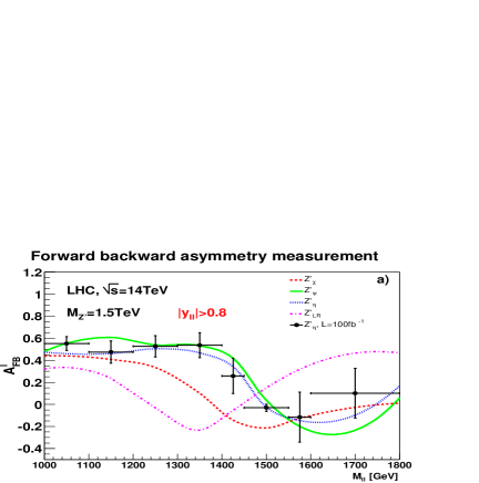
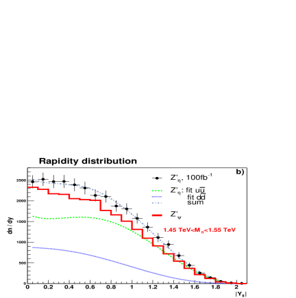
Figure 1: $\mathrm{A^{\ell}_{FB}}$ (a) as a function of $M_{\ell\ell}$ for four $Z^{\prime}$ models. The rapidity of the dilepton system is required to be larger than 0.8. The observable rapidity distribution for two $Z^{\prime}$ models is shown in (b), including the fit results which determine the types of $q\bar{q}$ fractions. A simulation of the statistical errors, including random fluctuations of the $Z^{\prime}_{\eta}$ model and with errors corresponding to a luminosity of 100 fb^-1 has been included in both plots.

In a next step, assuming that a particular model has been selected, one would like to know how well the parameter(s), like $\cos\beta$ or $\alpha_{LR}$ can be constrained. Figure 2 shows how the previously defined observables vary as the model parameters are varied. In the case of the $E_{6}$ model for instance, one finds that $\cos\beta$ can not always be determined unambiguously. Very similar results can be expected for different observables but using very different values for $\cos\beta$. Obviously, the combination of the various measurements, helps to reduce some ambiguities.

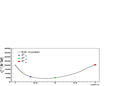
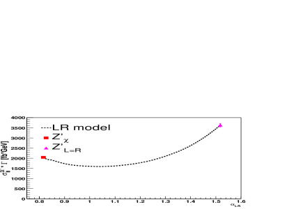
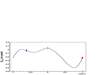
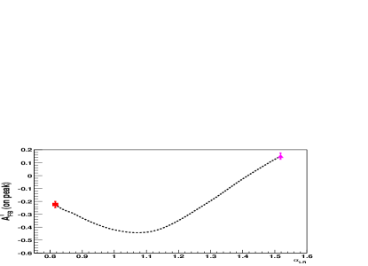
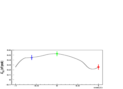
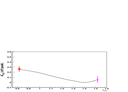
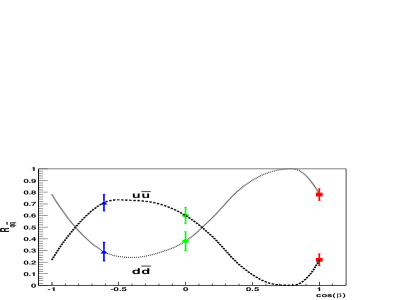
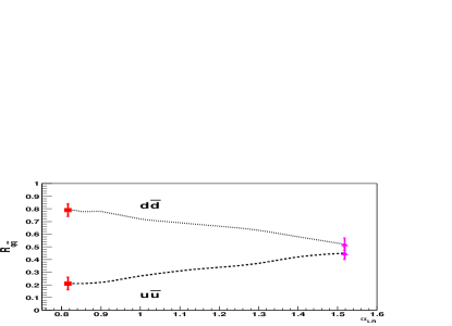
Figure 2: Variation of $\sigma^{3\Gamma}_{\ell\ell}\cdot\Gamma$, $A^{\rm on-peak}_{FB}$, $A^{\rm off-peak}_{FB}$ and the ratio $R_{q\bar{q}}$ as a function of the $E_{6}$ model parameter $\cos\beta$ (left) and the LR-model parameter $\alpha_{LR}$. The points corresponding the particular $Z^{\prime}$ models are also shown.

If the $Z^{\prime}$ mass is increased, the number of events decreases drastically and the differences between the models start to become covered within the statistical fluctuations. For the assumed luminosity of 100 fb^-1, one could still distinguish a $Z^{\prime}_{\chi}$ from a $Z^{\prime}_{LR}$ over a large parameter range and the $A_{FB}^{\ell}$ measurements provide some statistical significance up to $M_{Z^{\prime}}=2-2.5$ TeV. On the contrary, a $Z^{\prime}_{\eta}$ could be differentiated from a $Z^{\prime}_{\psi}$ only up to a $Z^{\prime}$ mass of at most 2 TeV, as in that case, the dependence of $A_{FB}^{\ell}$ on the $Z^{\prime}$ mass is almost identical for the two models.

4 CONCLUSIONS

A realistic simulation of the study of the properties of $Z^{\prime}$ bosons in $E_{6}$ and LR models has been performed for the LHC. We have shown that, in addition to the $Z^{\prime}$ production cross section times total decay width, the measurement of the forward-backward lepton charge asymmetry, both on the $Z^{\prime}$ peak and in the interference region, provide complementary information. We have also shown that a fit of the rapidity distribution can provide a sensitivity to the $Z^{\prime}$ couplings to up-type and down-type quarks. The combination of all these observables would allow us to discriminate between $Z^{\prime}$ bosons of different models or classes of models for masses up to 2–2.5 TeV, if a luminosity of 100 fb^-1 is collected.

References

- [1] B. C. Allanach, Softsusy: A c++ program for calculating supersymmetric spectra, Comput. Phys. Commun. 143 (2002) 305–331, [hep-ph/0104145].
- [2] H. Baer, F. E. Paige, S. D. Protopopescu, and X. Tata, Simulating supersymmetry with isajet 7.0 / isasusy 1.0, hep-ph/9305342.
- [3] A. Djouadi, J.-L. Kneur, and G. Moultaka, Suspect: A fortran code for the supersymmetric and higgs particle spectrum in the mssm, hep-ph/0211331.
- [4] S. Heinemeyer, W. Hollik, and G. Weiglein, Feynhiggs: A program for the calculation of the masses of the neutral cp-even higgs bosons in the mssm, Comput. Phys. Commun. 124 (2000) 76–89, [hep-ph/9812320].
- [5] W. Porod, Spheno, a program for calculating supersymmetric spectra, susy particle decays and susy particle production at e+ e- colliders, Comput. Phys. Commun. 153 (2003) 275–315, [hep-ph/0301101].
- [6] W. Beenakker, R. Hopker, and M. Spira, Prospino: A program for the production of supersymmetric particles in next-to-leading order qcd, hep-ph/9611232.
- [7] A. Djouadi, J. Kalinowski, and M. Spira, Hdecay: A program for higgs boson decays in the standard model and its supersymmetric extension, Comput. Phys. Commun. 108 (1998) 56–74, [hep-ph/9704448].
- [8] M. Muhlleitner, A. Djouadi, and Y. Mambrini, Sdecay: a fortran code for the decays of the supersymmetric particles in the mssm, hep-ph/0311167.
- [9] G. Belanger, F. Boudjema, A. Pukhov, and A. Semenov, micromegas: A program for calculating the relic density in the mssm, Comput. Phys. Commun. 149 (2002) 103–120, [hep-ph/0112278].
- [10] P. Gondolo et. al., Darksusy - a numerical package for supersymmetric dark matter calculations, astro-ph/0211238.
- [11] H. Baer, F. E. Paige, S. D. Protopopescu, and X. Tata, Isajet 7.48: A monte carlo event generator for p p, anti-p p, and e+ e- reactions, hep-ph/0001086.
- [12] G. Corcella et. al., Herwig 6: An event generator for hadron emission reactions with interfering gluons (including supersymmetric processes), JHEP 01 (2001) 010, [hep-ph/0011363].
- [13] T. Gleisberg et. al., Sherpa 1.alpha, a proof-of-concept version, hep-ph/0311263.
- [14] A. Pukhov et. al., Comphep: A package for evaluation of feynman diagrams and integration over multi-particle phase space. user’s manual for version 33, hep-ph/9908288.
- [15] T. Sjostrand et. al., High-energy-physics event generation with pythia 6.1, Comput. Phys. Commun. 135 (2001) 238–259, [hep-ph/0010017].
- [16] T. Sjostrand, L. Lonnblad, S. Mrenna, and P. Skands, Pythia 6.3 physics and manual, hep-ph/0308153.
- [17] Minami-Tateya Collaboration, H. Tanaka, M. Kuroda, T. Kaneko, M. Jimbo, and T. Kon, The grace system for the minimal supersymmetric standard model, Nucl. Instrum. Meth. A389 (1997) 295–298.
- [18] W. Kilian, Whizard 1.0: A generic monte-carlo integration and event generation package for multi-particle processes. manual, . LC-TOOL-2001-039.
- [19] P. Skands et. al., Susy les houches accord: Interfacing susy spectrum calculators, decay packages, and event generators, hep-ph/0311123.
- [20] M. Steinhauser, Leptonic contribution to the effective electromagnetic coupling constant up to three loops, Phys. Lett. B429 (1998) 158–161, [hep-ph/9803313].
- [21] D. Y. Bardin, M. Grunewald, and G. Passarino, Precision calculation project report, hep-ph/9902452.
- [22] Particle Data Group Collaboration, K. Hagiwara et. al., Review of particle physics, Phys. Rev. D66 (2002) 010001.
- [23] K. Melnikov and T. v. Ritbergen, The three-loop relation between the ms-bar and the pole quark masses, Phys. Lett. B482 (2000) 99–108, [hep-ph/9912391].
- [24] H. Baer, J. Ferrandis, K. Melnikov, and X. Tata, Relating bottom quark mass in dr-bar and ms-bar regularization schemes, Phys. Rev. D66 (2002) 074007, [hep-ph/0207126].
- [25] W. Siegel, Supersymmetric dimensional regularization via dimensional reduction, Phys. Lett. B84 (1979) 193.
- [26] D. M. Capper, D. R. T. Jones, and P. van Nieuwenhuizen, Regularization by dimensional reduction of supersymmetric and nonsupersymmetric gauge theories, Nucl. Phys. B167 (1980) 479.
- [27] I. Jack, D. R. T. Jones, S. P. Martin, M. T. Vaughn, and Y. Yamada, Decoupling of the epsilon scalar mass in softly broken supersymmetry, Phys. Rev. D50 (1994) 5481–5483, [hep-ph/9407291].
- [28] W. Beenakker, H. Kuijf, W. L. van Neerven, and J. Smith, Qcd corrections to heavy quark production in p anti-p collisions, Phys. Rev. D40 (1989) 54–82.
- [29] S. P. Martin and M. T. Vaughn, Regularization dependence of running couplings in softly broken supersymmetry, Phys. Lett. B318 (1993) 331–337, [hep-ph/9308222].
- [30] B. C. Allanach et. al., The snowmass points and slopes: Benchmarks for susy searches, Eur. Phys. J. C25 (2002) 113–123, [hep-ph/0202233].
- [31] B. C. Allanach, S. Kraml, and W. Porod, Theoretical uncertainties in sparticle mass predictions from computational tools, JHEP 03 (2003) 016, [hep-ph/0302102].
- [32] I. Jack, D. R. T. Jones, and A. F. Kord, Three loop soft running, benchmark points and semi-perturbative unification, hep-ph/0308231.
- [33] H. Baer, F. E. Paige, S. D. Protopescu, and X. Tata, Isajet 7.69: A monte carlo event generator for p p, anti-p p, and e+ e- reactions, hep-ph/0312045.
- [34] B. C. Allanach, J. P. J. Hetherington, M. A. Parker, and B. R. Webber, Naturalness reach of the large hadron collider in minimal supergravity, JHEP 08 (2000) 017, [hep-ph/0005186].
- [35] A. B., G. Belanger, F. Boudjema, and A. Pukhov in preparation.
- [36] G. A. Blair, W. Porod, and P. M. Zerwas, Reconstructing supersymmetric theories at high energy scales, Phys. Rev. D63 (2001) 017703, [hep-ph/0007107].
- [37] G. A. Blair, W. Porod, and P. M. Zerwas, The reconstruction of supersymmetric theories at high energy scales, Eur. Phys. J. C27 (2003) 263–281, [hep-ph/0210058].
- [38] K. Desch, J. Kalinowski, G. Moortgat-Pick, M. M. Nojiri, and G. Polesello, Susy parameter determination in combined analyses at lhc/lc, hep-ph/0312069.
- [39] G. Ganis, Msmlib (unpublished), .
- [40] V. D. Barger et. al., Cp-violating phases in susy, electric dipole moments, and linear colliders, Phys. Rev. D64 (2001) 056007, [hep-ph/0101106].
- [41] W. Beenakker, R. Hopker, M. Spira, and P. M. Zerwas, Squark and gluino production at hadron colliders, Nucl. Phys. B492 (1997) 51–103, [hep-ph/9610490].
- [42] W. Beenakker, M. Kramer, T. Plehn, M. Spira, and P. M. Zerwas, Stop production at hadron colliders, Nucl. Phys. B515 (1998) 3–14, [hep-ph/9710451].
- [43] W. Beenakker et. al., The production of charginos/neutralinos and sleptons at hadron colliders, Phys. Rev. Lett. 83 (1999) 3780–3783, [hep-ph/9906298].
- [44] F. James and M. Roos, ’minuit’ a system for function minimization and analysis of the parameter errors and correlations, Comput. Phys. Commun. 10 (1975) 343–367.
- [45] N. Ghodbane and H.-U. Martyn, Compilation of susy particle spectra from snowmass 2001 benchmark models, hep-ph/0201233.
- [46] M. Drees and S. P. Martin, Implications of susy model building, hep-ph/9504324.
- [47] MSSM Working Group Collaboration, A. Djouadi et. al., The minimal supersymmetric standard model: Group summary report, hep-ph/9901246.
- [48] A. Djouadi, M. Spira, and P. M. Zerwas, Qcd corrections to hadronic higgs decays, Z. Phys. C70 (1996) 427–434, [hep-ph/9511344].
- [49] S. Kraml, H. Eberl, A. Bartl, W. Majerotto, and W. Porod, Susy–qcd corrections to scalar quark decays into charginos and neutralinos, Phys. Lett. B386 (1996) 175–182, [hep-ph/9605412].
- [50] A. Djouadi, W. Hollik, and C. Junger, Qcd corrections to scalar quark decays, Phys. Rev. D55 (1997) 6975–6985, [hep-ph/9609419].
- [51] A. Arhrib, A. Djouadi, W. Hollik, and C. Junger, Susy higgs boson decays into scalar quarks: Qcd corrections, Phys. Rev. D57 (1998) 5860–5870, [hep-ph/9702426].
- [52] A. Bartl et. al., Susy-qcd corrections to stop and sbottom decays into higgs bosons, Phys. Rev. D59 (1999) 115007, [hep-ph/9806299].
- [53] A. Bartl et. al., Susy-qcd corrections to stop and sbottom decays into w and z bosons, Phys. Lett. B419 (1998) 243–252, [hep-ph/9710286].
- [54] A. Bartl et. al., Bosonic decays of stop2 and sbottom2, Phys. Lett. B435 (1998) 118–124, [hep-ph/9804265].
- [55] W. Beenakker, R. Hopker, and P. M. Zerwas, Susy-qcd decays of squarks and gluinos, Phys. Lett. B378 (1996) 159–166, [hep-ph/9602378].
- [56] W. Beenakker, R. Hopker, T. Plehn, and P. M. Zerwas, Stop decays in susy-qcd, Z. Phys. C75 (1997) 349–356, [hep-ph/9610313].
- [57] H. E. Haber and D. Wyler, Radiative neutralino decay., Nucl. Phys. B323 (1989) 267.
- [58] S. Ambrosanio and B. Mele, Neutralino decays in the minimal supersymmetric standard model, Phys. Rev. D53 (1996) 2541–2562, [hep-ph/9508237].
- [59] S. Ambrosanio and B. Mele, Supersymmetric scenarios with dominant radiative neutralino decay, Phys. Rev. D55 (1997) 1399–1417, [hep-ph/9609212].
- [60] H. Baer and T. Krupovnickas, Radiative neutralino decay in supersymmetric models, JHEP 09 (2002) 038, [hep-ph/0208277].
- [61] E. Ma and G.-G. Wong, Two-body radiative gluino decays., Mod. Phys. Lett. A3 (1988) 1561.
- [62] R. Barbieri, G. Gamberini, G. F. Giudice, and G. Ridolfi, Constraining supergravity models from gluino production, Nucl. Phys. B301 (1988) 15.
- [63] H. Baer, X. Tata, and J. Woodside, Searching for 100-gev - 300-gev gluinos at the tevatron and ssc, Phys. Rev. D42 (1990) 1568–1576.
- [64] K.-I. Hikasa and M. Kobayashi, Light scalar top at e+ e- colliders, Phys. Rev. D36 (1987) 724.
- [65] A. Bartl, W. Majerotto, and W. Porod, Squark and gluino decays for large tan beta, Z. Phys. C64 (1994) 499–508.
- [66] A. Bartl, W. Majerotto, and W. Porod, Large higgs boson exchange contribution in three-body neutralino decays, Phys. Lett. B465 (1999) 187–192, [hep-ph/9907377].
- [67] H. Baer, C.-H. Chen, M. Drees, F. Paige, and X. Tata, Collider phenomenology for supersymmetry at large , Phys. Rev. Lett. 79 (1997) 986–989, [hep-ph/9704457].
- [68] H. Baer, C.-H. Chen, M. Drees, F. Paige, and X. Tata Phys. Rev. D59 (1999) 055014, [hep-ph/9809223].
- [69] A. Djouadi, Y. Mambrini, and M. Muhlleitner, Probing minimal supergravity at the cern lhc for large , Eur. Phys. J. C20 (2001) 563–584, [hep-ph/0104115].
- [70] W. Porod, The decays gluino stop1 b-quark w and gluino stop1 c-quark and phenomenological implications in supersymmetric theories, JHEP 05 (2002) 030, [hep-ph/0202259].
- [71] A. Datta, A. Djouadi, M. Guchait, and Y. Mambrini, Charged higgs production from susy particle cascade decays at the lhc, Phys. Rev. D65 (2002) 015007, [hep-ph/0107271].
- [72] W. Porod and T. Wohrmann, Higher order top squark decays, Phys. Rev. D55 (1997) 2907–2917, [hep-ph/9608472].
- [73] W. Porod, More on higher order decays of the lighter top squark, Phys. Rev. D59 (1999) 095009, [hep-ph/9812230].
- [74] A. Datta, M. Guchait, and K. K. Jeong, Stop squark search at tevatron in the light slepton scenario, Int. J. Mod. Phys. A14 (1999) 2239–2256, [hep-ph/9903214].
- [75] A. Djouadi, M. Guchait, and Y. Mambrini, Scalar top quarks at the run ii of the tevatron in the high regime, Phys. Rev. D64 (2001) 095014, [hep-ph/0105108].
- [76] A. Djouadi and Y. Mambrini, Three-body decays of susy particles, Phys. Lett. B493 (2000) 120–126, [hep-ph/0007174].
- [77] A. Djouadi and Y. Mambrini, Three-body decays of top and bottom squarks, Phys. Rev. D63 (2001) 115005, [hep-ph/0011364].
- [78] C. Boehm, A. Djouadi, and Y. Mambrini, Decays of the lightest top squark, Phys. Rev. D61 (2000) 095006, [hep-ph/9907428].
- [79] T. A. Collaboration, Detector and physics performance technical design report, CERN/LHCC/99-14 ATLAS TDR 14 (1999).
- [80] I. Hinchliffe, F. E. Paige, M. D. Shapiro, J. Soderqvist, and W. Yao, Precision susy measurements at lhc, Phys. Rev. D55 (1997) 5520–5540, [hep-ph/9610544].
- [81] I. Hinchliffe and F. E. Paige, Measurements in sugra models with large tan(beta) at lhc, Phys. Rev. D61 (2000) 095011, [hep-ph/9907519].
- [82] H. Bachacou, I. Hinchliffe, and F. E. Paige, Measurements of masses in sugra models at lhc, Phys. Rev. D62 (2000) 015009, [hep-ph/9907518].
- [83] B. C. Allanach, C. G. Lester, M. A. Parker, and B. R. Webber, Measuring sparticle masses in non-universal string inspired models at the lhc, JHEP 09 (2000) 004, [hep-ph/0007009].
- [84] CMS Collaboration, S. Abdullin et. al., Discovery potential for supersymmetry in cms, J. Phys. G28 (2002) 469, [hep-ph/9806366].
- [85] B. Gjelste et. al., A detailed analysis of the measurement of susy masses with the atlas detector at the lhc, in LHC/LC Study group document (G. Weiglein, ed.), DESY, 2003.
- [86] ATLAS Collaboration, F. Brochu et. al., Full supersymmetry simulation in dc1, . ATLAS NOTE.
- [87] S. Moretti, K. Odagiri, P. Richardson, M. H. Seymour, and B. R. Webber, Implementation of supersymmetric processes in the herwig event generator, JHEP 04 (2002) 028, [hep-ph/0204123].
- [88] E. Richter-Was, D. Froidevaux, and L. Poggioli, Atlfast 2.0: a fast simulation package for atlas, . ATLAS NOTE ATL-PHYS-98-131.
- [89] M. M. Nojiri, G. Polesello, and D. R. Tovey, Proposal for a new reconstruction technique for susy processes at the lhc, in Contribution to these proceedings.
- [90] J. Hisano, K. Kawagoe, and M. M. Nojiri, A detailed study of the gluino decay into the third generation squarks at the cern lhc, Phys. Rev. D68 (2003) 035007, [hep-ph/0304214].
- [91] T. Tsukamoto, K. Fujii, H. Murayama, M. Yamaguchi, and Y. Okada, Precision study of supersymmetry at future linear e+ e- colliders, Phys. Rev. D51 (1995) 3153–3171.
- [92] J. L. Feng, M. E. Peskin, H. Murayama, and X. Tata, Testing supersymmetry at the next linear collider, Phys. Rev. D52 (1995) 1418–1432, [hep-ph/9502260].
- [93] S. Y. Choi, J. Kalinowski, G. Moortgat-Pick, and P. M. Zerwas, Analysis of the neutralino system in supersymmetric theories, Eur. Phys. J. C22 (2001) 563–579, [hep-ph/0108117].
- [94] S. Y. Choi, J. Kalinowski, G. Moortgat-Pick, and P. M. Zerwas, Analysis of the neutralino system in supersymmetric theories. (addendum), hep-ph/0202039.
- [95] S. Y. Choi et. al., Reconstructing the chargino system at e+ e- linear colliders, Eur. Phys. J. C14 (2000) 535–546, [hep-ph/0002033].
- [96] S. Y. Choi, A. Djouadi, H. K. Dreiner, J. Kalinowski, and P. M. Zerwas, Chargino pair production in e+ e- collisions, Eur. Phys. J. C7 (1999) 123–134, [hep-ph/9806279].
- [97] K. Desch, J. Kalinowski, G. Moortgat-Pick, M. M. Nojiri, and G. Polesello, Susy parameter determination in combined analyses at lhc/lc, hep-ph/0312069.
- [98] E. Boos et. al., Polarisation in sfermion decays: Determining tan(beta) and trilinear couplings, Eur. Phys. J. C30 (2003) 395–407, [hep-ph/0303110].
- [99] V. D. Barger, T. Han, and J. Jiang, tan(beta) determination from heavy higgs boson production at linear colliders, Phys. Rev. D63 (2001) 075002, [hep-ph/0006223].
- [100] J. Gunion, T. Han, J. Jiang, and A. Sopczak, Determining tan(beta) with neutral and charged higgs bosons at a future e+ e- linear collider, Phys. Lett. B565 (2003) 42–60, [hep-ph/0212151].
- [101] M. M. Nojiri, G. Polesello, and D. R. Tovey, Measuring the mass of the lightest chargino at the cern lhc, Contribution to these proceedings (2004).
- [102] S. Abdullin, D. Denegri, and F. Moortgat, Observability of mssm higgs bosons via sparticle decay modes in cms, CMS NOTE-2001/042 — PHYSICS.
- [103] M. M. Nojiri, G. Polesello, and D. R. Tovey, Proposal for a new reconstruction technique for SUSY processes at the LHC, hep-ph/0312317.
- [104] E. Richter-Was, D. Froidevaux, and L. Poggioli, ATLFAST 2.0: a fast simulation package for ATLAS, Tech. Rep. ATL-PHYS-98-131, 1998.
- [105] D. J. C. MacKay, Information Theory, Inference and Learning Algorithms. Cambridge University Press, 2004.
- [106] K. Kawagoe, T. Kobayashi, M. M. Nojiri, and A. Ochi, Study of the gauge mediation signal with non-pointing photons at the cern lhc, hep-ph/0309031.
- [107] ATLAS Collaboration, A. Airapetian et. al. CERN-LHCC-96-40.
- [108] ATLAS Collaboration, A. Artamonov, A. Dell’Acqua, D. Froidevaux, M. Nessi, P. Nevski, and G. Poulard. ATLAS-SOFT/95-14c.
- [109] Super-Kamiokande Collaboration, Y. Fukuda et. al., Evidence for oscillation of atmospheric neutrinos, Phys. Rev. Lett. 81 (1998) 1562–1567, [hep-ex/9807003].
- [110] Super-Kamiokande Collaboration, S. Fukuda et. al., Solar b-8 and hep neutrino measurements from 1258 days of super-kamiokande data, Phys. Rev. Lett. 86 (2001) 5651–5655, [hep-ex/0103032].
- [111] SNO Collaboration, Q. R. Ahmad et. al., Measurement of the rate of nu/e + d –¿ p + p + e- interactions produced by b-8 solar neutrinos at the sudbury neutrino observatory, Phys. Rev. Lett. 87 (2001) 071301, [nucl-ex/0106015].
- [112] KamLAND Collaboration, K. Eguchi et. al., First results from kamland: Evidence for reactor anti-neutrino disappearance, Phys. Rev. Lett. 90 (2003) 021802, [hep-ex/0212021].
- [113] M. Gell-Mann, P. Ramond, and R. Slansky, Complex spinors and unified theories, . Print-80-0576 (CERN).
- [114] T. Yanagida, Nucleon decay in supergrand unification, Prog. Theor. Phys. 64 (1980) 1103.
- [115] R. N. Mohapatra and G. Senjanovic, Neutrino masses and mixings in gauge models with spontaneous parity violation, Phys. Rev. Lett. 44 (1980) 912.
- [116] J. C. Romão, M. A. Díaz, M. Hirsch, W. Porod, and J. W. F. Valle, A supersymmetric solution to the solar and atmospheric neutrino problems, Phys. Rev. D61 (2000) 071703, [hep-ph/9907499].
- [117] M. Hirsch, M. A. Díaz, W. Porod, J. C. Romão, and J. W. F. Valle, Neutrino masses and mixings from supersymmetry with bilinear r parity violation: A theory for solar and atmospheric neutrino oscillations, Phys. Rev. D62 (2000) 113008, [hep-ph/0004115].
- [118] M. A. Díaz, M. Hirsch, W. Porod, J. C. Romão, and J. W. F. Valle, Solar neutrino masses and mixing from bilinear r parity broken supersymmetry: Analytical versus numerical results, Phys. Rev. D68 (2003) 013009, [hep-ph/0302021].
- [119] B. Mukhopadhyaya, S. Roy, and F. Vissani, Correlation between neutrino oscillations and collider signals of supersymmetry in an r-parity violating model, Phys. Lett. B443 (1998) 191–195, [hep-ph/9808265].
- [120] W. Porod, M. Hirsch, J. Romão, and J. W. F. Valle, Testing neutrino mixing at future collider experiments, Phys. Rev. D63 (2001) 115004, [hep-ph/0011248].
- [121] M. Hirsch, W. Porod, J. C. Romão, and J. W. F. Valle, Probing neutrino properties with charged scalar lepton decays, Phys. Rev. D66 (2002) 095006, [hep-ph/0207334].
- [122] M. Hirsch and W. Porod, Neutrino properties and the decay of the lightest supersymmetric particle, Phys. Rev. D68 (2003) 115007, [hep-ph/0307364].
- [123] C. Collaboration. CERN-LHCC-02-26.
- [124] B. C. Allanach and K. Sridhar, Combined fits to the supersymmetric explanation of anomalous lepton gamma missing e(t) events, Phys. Lett. B551 (2003) 343–350, [hep-ph/0210375].
- [125] B. C. Allanach, S. Lola, and K. Sridhar, Explaining anomalous cdf mu gamma missing-e(t) events with supersymmetry, Phys. Rev. Lett. 89 (2002) 011801, [hep-ph/0111014].
- [126] B. C. Allanach, S. Lola, and K. Sridhar, Investigating the supersymmetric explanation of anomalous cdf lepton(s) photon(s) missing-e(t) events, JHEP 04 (2002) 002, [hep-ph/0112321].
- [127] V. D. Barger, G. F. Giudice, and T. Han, Some new aspects of supersymmetry r parity violating interactions, Phys. Rev. D40 (1989) 2987.
- [128] B. C. Allanach, A. Dedes, and H. K. Dreiner, Bounds on r-parity violating couplings at the weak scale and at the gut scale, Phys. Rev. D60 (1999) 075014, [hep-ph/9906209].
- [129] F. E. Paige, S. D. Protopescu, H. Baer, and X. Tata, Isajet 7.40: A monte carlo event generator for p p, anti-p p, and e+ e- reactions, hep-ph/9810440.
- [130] G. Corcella et. al., Herwig 6.3 release note, hep-ph/0107071.
- [131] B. C. Allanach, M. Guchait, and K. Sridhar, Resonant slepton production at the lhc in models with an ultralight gravitino, hep-ph/0311254.
- [132] L. Randall and R. Sundrum, A large mass hierarchy from a small extra dimension, Phys. Rev. Lett. 83 (1999) 3370–3373, [hep-ph/9905221].
- [133] H. Davoudiasl, J. L. Hewett, and T. G. Rizzo, Warped phenomenology, Phys. Rev. Lett. 84 (2000) 2080, [hep-ph/9909255].
- [134] H. Davoudiasl, J. L. Hewett, and T. G. Rizzo, Bulk gauge fields in the randall-sundrum model, Phys. Lett. B473 (2000) 43–49, [hep-ph/9911262].
- [135] H. Davoudiasl, J. L. Hewett, and T. G. Rizzo, Experimental probes of localized gravity: On and off the wall, Phys. Rev. D63 (2001) 075004, [hep-ph/0006041].
- [136] G. F. Giudice, R. Rattazzi, and J. D. Wells, Graviscalars from higher dimensional metrics and curvature higgs mixing, Nucl. Phys. B 595 (2001) 250, [hep-ph/0002178].
- [137] C. Csaki, M. Graesser, and G. Kribs, Radion dynamics and electroweak physics, Phys. Rev. D63 (2001) 065002, [hep-th/0008151].
- [138] J. L. Hewett and T. G. Rizzo, Shifts in the properties of the higgs boson from radion mixing, JHEP 08 (2003) 028, [hep-ph/0202155].
- [139] D. Dominici, B. Grzadkowski, J. F. Gunion, and T. M., The scalar sector of the randall-sundrum model, Nucl. Phys. B671 (2003) 243–292, [hep-ph/0206192].
- [140] R. Altendorfer, J. Bagger, and D. Nemeschansky, Supersymmetric randall-sundrum scenario, Phys. Rev. D63 (2001) 125025, [hep-th/0003117].
- [141] T. Gherghetta and A. Pomarol, Bulk fields and supersymmetry in a slice of ads, Nucl. Phys. B586 (2000) 141–162, [hep-ph/0003129].
- [142] W. Goldberger and M. Wise, Modulus stabilization with bulk fields, Phys. Rev. Lett. 83 (1999) 4922–4925, [hep-ph/9907447].
- [143] M. Carena, H. E. Haber, H. E. Logan, and S. Mrenna, Distinguishing a mssm higgs boson from the sm higgs boson at a linear collider, Phys. Rev. D65 (2002) 055005, [hep-ph/0106116].
- [144] T. Han, G. Kribs, and B. McElrath, Radion effects on unitarity in gauge-boson scattering, Phys. Rev. D64 (2001) 076003, [hep-ph/0104074].
- [145] L. Randall and R. Sundrum, An alternative to compactification, Phys. Rev. Lett. 83 (1999) 4690–4693, [hep-th/9906064].
- [146] M. Chaichian, A. Datta, K. Huitu, and Z. h. Yu, Radion and higgs mixing at the lhc, Phys.Lett. B 524 (2002) 161, [hep-ph/0110035].
- [147] M. Battaglia, S. D. Curtis, A. D. Roeck, D. Dominici, and G. J. F., On the complementarity of higgs and radion searches at lhc, Phys. Lett. B568 (2003) 92–102, [hep-ph/0304245].
- [148] G. Azuelos, D. Cavalli, H. Przysiezniak, and L. Vacavant SN-ATLAS-2002-019.
- [149] T. Sjostrand, L. Lonnblad, and S. Mrenna, Pythia 6.2: Physics and manual, hep-ph/0108264.
- [150] CERN/LHCC 2000-38, CMS TDR 6.1, 15 December, 2000.
- [151] CERN/LHCC/2002-26, CMS TDR 6.2, 15 December, 2002.
- [152] F. Maltoni and T. Stelzer, Madevent: Automatic event generation with madgraph, JHEP 02 (2003) 027, [hep-ph/0208156].
- [153] T. Stelzer and W. F. Long, Automatic generation of tree level helicity amplitudes, Comput. Phys. Commun. 81 (1994) 357–371, [hep-ph/9401258].
- [154] G. Segneri and F. Palla CMS NOTE 2002/046.
- [155] J. Campbell, R. K. Ellis, and D. Rainwater, Next-to-leading order qcd predictions for w+2j and z+2j production at the cern lhc, Phys. Rev. D68 (2003) 094021, [hep-ph/0308195].
- [156] D. Chakraborty, J. Konigsberg, and D. Rainwater, Review of top quark physics, hep-ph/0303092.
- [157] CERN 2000-004, 9 May, 2000.
- [158] S. Abdullin et. al. CMS TN/94-180.
- [159] N. Arkani-Hamed, S. Dimopoulos, and G. R. Dvali, The hierarchy problem and new dimensions at a millimeter, Phys. Lett. B429 (1998) 263–272, [hep-ph/9803315].
- [160] I. Antoniadis, N. Arkani-Hamed, S. Dimopoulos, and G. R. Dvali, New dimensions at a millimeter to a fermi and superstrings at a tev, Phys. Lett. B436 (1998) 257–263, [hep-ph/9804398].
- [161] J. D. Wells, Extra dimensions and the universal suppression of higgs boson observables at high energy colliders, hep-ph/0205328.
- [162] G. F. Giudice, R. Rattazzi, and J. D. Wells, Quantum gravity and extra dimensions at high-energy colliders, Nucl. Phys. B544 (1999) 3–38.
- [163] S. Abdullin et. al. CMS note-2003/033.
- [164] B. Di Girolamo, A. Nikitenko, L. Neukermans, K. Mazumdar, and D. Zeppenfeld. Prepared for Workshop on Physics at TeV Colliders, Les Houches, France, 21 May - 1 Jun 2001.
- [165] L. Vacavant and I. Hinchliffe, Signals of models with large extra dimensions in atlas, J. Phys. G27 (2001) 1839–1850.
- [166] M. Schumacher, Note, . LC-PHSM 2003-096.
- [167] K. R. Dienes, E. Dudas, and T. Gherghetta, Extra spacetime dimensions and unification, Phys. Lett. B436 (1998) 55–65, [hep-ph/9803466].
- [168] M. Masip and A. Pomarol, Effects of sm kaluza-klein excitations on electroweak observables, Phys. Rev. D60 (1999) 096005, [hep-ph/9902467].
- [169] A. Aranda, C. Balazs, and J. L. Diaz-Cruz, Where is the higgs boson?, Nucl. Phys. B670 (2003) 90–102, [hep-ph/0212133].
- [170] R. W. Assmann et. al., A 3-tev e+ e- linear collider based on clic technology, . SLAC-REPRINT-2000-096.
- [171] J. Polchinski, Dirichlet-branes and ramond-ramond charges, Phys. Rev. Lett. 75 (1995) 4724–4727, [hep-th/9510017].
- [172] P. Horava and E. Witten, Eleven-dimensional supergravity on a manifold with boundary, Nucl. Phys. B475 (1996) 94–114, [hep-th/9603142].
- [173] A. Pomarol and M. Quiros, The standard model from extra dimensions, Phys. Lett. B438 (1998) 255–260, [hep-ph/9806263].
- [174] I. Antoniadis, S. Dimopoulos, A. Pomarol, and M. Quiros, Soft masses in theories with supersymmetry breaking by tev-compactification, Nucl. Phys. B544 (1999) 503–519, [hep-ph/9810410].
- [175] A. Delgado, A. Pomarol, and M. Quiros, Supersymmetry and electroweak breaking from extra dimensions at the tev-scale, Phys. Rev. D60 (1999) 095008, [hep-ph/9812489].
- [176] C. D. Carone, Electroweak constraints on extended models with extra dimensions, Phys. Rev. D61 (2000) 015008, [hep-ph/9907362].
- [177] K. R. Dienes, E. Dudas, and T. Gherghetta, Grand unification at intermediate mass scales through extra dimensions, Nucl. Phys. B537 (1999) 47–108, [hep-ph/9806292].
- [178] D. A. Dicus, C. D. McMullen, and S. Nandi, Collider implications of kaluza-klein excitations of the gluons, Phys. Rev. D65 (2002) 076007, [hep-ph/0012259].
- [179] C. Balazs and B. Laforge, Probing tev-scale gauge unification by hadronic collisions, Phys. Lett. B525 (2002) 219–224, [hep-ph/0110217].
- [180] H. Tao, H. E. Logan, B. Mc. Elrath and L.-T. Wang, Phenomenology of the little Higgs model, Phys. Rev. D67 (2003) 095044, [hep-ph/0301040].
- [181] M. Dittmar, A.-S. Nicollerat, and A. Djouadi, Z’ studies at the lhc: An update, hep-ph/0307020.
- [182] A. Djouadi, A. Leike, T. Riemann, D. Schaile, and C. Verzegnassi, Signals of new gauge bosons at future e+ e- colliders, Z. Phys. C56 (1992) 289–300.
- [183] M. Dittmar, Neutral current interference in the tev region: The experimental sensitivity at the lhc, Phys. Rev. D55 (1997) 161–166, [hep-ex/9606002].
- [184] M. Dittmar, F. Pauss, and D. Zurcher, Towards a precise parton luminosity determination at the cern lhc, Phys. Rev. D56 (1997) 7284–7290, [hep-ex/9705004].
- [185] F. del Aguila, M. Cvetic, and P. Langacker, Determination of z-prime gauge couplings to quarks and leptons at future hadron colliders, Phys. Rev. D48 (1993) 969–973, [hep-ph/9303299].