Smooth hybrid inflation in supergravity
with a running spectral index and early star formation

Abstract

It is shown that in a smooth hybrid inflation model in supergravity adiabatic fluctuations with a running spectral index with $n_{s}>1$ on a large scale and $n_{s}<1$ on a smaller scale can be naturally generated, as favored by the first-year data of WMAP. It is due to the balance between the nonrenormalizable term in the superpotential and the supergravity effect. However, since smooth hybrid inflation does not last long enough to reproduce the central value of observation, we invoke new inflation after the first inflation. Its initial condition is set dynamically during smooth hybrid inflation and the spectrum of fluctuations generated in this regime can have an appropriate shape to realize early star formation as found by WMAP. Hence two new features of WMAP observations are theoretically explained in a unified manner.

I Introduction

The observation of cosmic microwave background anisotropy by the Wilkinson Microwave Anisotropy Probe (WMAP) has determined cosmological parameters with a good accuracy. They have shown that the geometry of our universe is practically flat and that the energy density of the universe is dominated by dark energy and compensated by dark matter and a small amount of baryons Bennett ; Spergel . Furthermore, primordial density fluctuations are shown to be adiabatic, Gaussian, and nearly scale invariant, which suggests that they were produced during inflation Spergel ; Peiris . Thus, the so-called concordance model was confirmed.

Going into the details, however, we find several interesting features that may not be reconciled with a simple scale-invariant spectrum : namely, an early period of re-ionization (see, e.g., YY for a possible explanation), a lack of fluctuation power on the largest scale, the running spectral index of fluctuations, $n_{s}$ YY ; FLZZ ; KS ; KYY , and the oscillatory behavior of multipoles which may suggest oscillations in the primordial power spectrum kogo . Of course, these properties may disappear eventually when the observations are improved. But it is still important to consider a model to explain them at the present stage. In this paper, we discuss the running of spectral index from $n_{s}>1$ on a large scale to $n_{s}<1$ on a smaller scale. More concretely, it is shown that $n_{s}=1.13\pm 0.08$ and $dn_{s}/d\ln k=-0.055^{+0.028}_{-0.029}$ on the scale $k_{0}=0.002\,{\rm Mpc}^{-1}$ Peiris .

Among the three types of slow-roll inflation–namely, new newinf , chaotic chaoinf , and hybrid hybrid inflation–the first two scenarios predict fluctuations with $n_{s}<1$ while hybrid inflation can realize both those with $n_{s}>1$ and $n_{s}<1$. Although it is fairly easy to construct a model whose spectral index runs from $n_{s}<1$ to $n_{s}>1$ for decreasing length scales, it is quite nontrivial to realize the opposite running. The hybrid inflation model in supergravity proposed by Linde and Riotto LR is an exception in which the desired feature is realized due to the contributions to the potential from both one-loop effects and supergravity effects. Based on this observation, some models have been discussed in an attempt to reproduce the results of the WMAP, but it turned out that the large enough running is incompatible with long enough inflation KS ; KYY ; YY . This is because the Yukawa coupling constant must be relatively small for sufficient inflation while it must be large for large running.

This problem was first solved in KYY by introducing another inflaton whose appropriate initial condition is automatically prepared during the hybrid inflation regime IY ; Kawasaki:1998vx ; Kanazawa:1999ag . This model, however, could not reproduce the central value of the running spectral index obtained by WMAP data but could realize the feature only at the one-sigma level because small-scale fluctuations tend to be too large and we have to hide the corresponding scales in an unobservable region. More serious is the problem of the initial condition common to other hybrid inflation models that only a very limited initial configuration can lead to inflation hybridinit . Both these problems have been solved in the chaotic hybrid new inflation model in supergravity proposed by us YY , which can also realize mildly large fluctuations in the appropriate scales to realize early star formation to help early re-ionization.

In the present paper we present another possible mechanism to realize running spectral index from $n_{s}>1$ to $n_{s}<1$ for decreasing length scale: namely, smooth hybrid inflation in supergravity. This scenario was originally proposed by Lazarides and Panagiotakopoulos smooth ; shift ; SS , in which nonrenormalizable terms are introduced and gauge symmetry remains broken even during hybrid inflation. Thus, topological defects are not produced at the end of inflation. In this paper, we discuss smooth hybrid inflation in supergravity and investigate whether the running spectral index is obtained with the desired property. As will be shown shortly, the spectral index runs from $n_{s}>1$ on a large scale to $n_{s}<1$ on a smaller scale without resorting to the one-loop effects unlike our previous models KYY ; YY . Another merit of this scenario is that it can be realized with natural initial conditions in minimal supergravity smoothini . We find, however, that we cannot yield large enough $e$-folds of inflation with large enough running of the spectral index whichever power of the nonrenormalizable term we may choose. So another inflation is required after smooth hybrid inflation as with the case with our previous models YY ; KYY . Adopting new inflation as the second inflation, we make a specific model of smooth hybrid new inflation in supergravity. Generally speaking, density fluctuations produced at the onset of new inflation become large. Actually, as shown in KYY , if we consider usual hybrid inflation before new inflation, the density fluctuations produced during new inflation are too large, which may cause an overproduction problem of dark halos. However, in the case of smooth hybrid inflation, they can be adequately large, which may be helpful for early star formation. Thus this scenario can also solve the two problems of the hybrid new inflation model of KYY just as the chaotic hybrid new inflation model YY does. Which of these two remaining models is more appropriate may be judged by future observations from the presence or the absence of cosmic strings, because the latter model predicts cosmic strings with their energy scale close to the current observational upper bound imposed by cosmic microwave background radiation. On the other hand, it has been claimed that long cosmic strings lose their energy directly into particles instead of string loops Vincent:1996rb . Although we understand this issue is still in dispute moore , if it turned out to be true, it would rule out our previous model because too many high-energy cosmic rays would be produced Wichoski:1998kh .

The rest of the paper is organized as follows. In Sec. II we consider smooth hybrid inflation in supergravity and investigate the spectral nature of produced density fluctuations. Then in Sec. III, after reviewing new inflation, we introduce smooth hybrid new inflation, and investigate their dynamics and density fluctuations. Section IV is devoted to a discussion and future outlook. In this paper, we set $M_{G}=2.4\times 10^{18}$ GeV to be unity otherwise stated.

II Smooth hybrid inflation in supergravity

First we introduce smooth hybrid inflation in supergravity smooth ; SS . The superpotential is given by

$$W_{H}=S\left(-\mu^{2}+\frac{(\overline{\Psi}\Psi)^{m}}{M^{2(m-1)}}\right),$$ (1)

where $\Psi$ and $\overline{\Psi}$ are a conjugate pair of superfields transforming as nontrivial representations of some gauge group, under which a superfield $S$ is singlet. $\mu$ is the energy scale of hybrid inflation which may be related to the grand unified theory, and $M$ is a cutoff scale which controls the nonrenormalizable term. $m$ is an integer with $m\geq 2$. This superpotential possesses two symmetries. One is the $R$ symmetry under which they are transformed as $S\longrightarrow e^{2i\alpha}S$, $\Psi\longrightarrow e^{2i\alpha}\Psi$, $\overline{\Psi}\longrightarrow e^{-2i\alpha}\overline{\Psi}$, and $W_{H}\longrightarrow e^{2i\alpha}W_{H}$. The other is a discrete symmetry $Z_{m}$ under which $\overline{\Psi}\Psi$ has unit charge. The $R$-invariant Kähler potential is given by

$$K_{H}=|S|^{2}+|\Psi|^{2}+|\overline{\Psi}|^{2}+\cdots,$$ (2)

where we have retained only the minimal terms. But the essential result remains intact even if we take higher-order terms into account.

The potential of scalar fields is given by

$$V_{H}(S,\Psi,\overline{\Psi}) = e^{|S|^{2}+|\Psi|^{2}+|\overline{\Psi}|^{2}}\left\{(1-|S|^{2}+|S|^{4})\left|-\mu^{2}+\frac{(\overline{\Psi}\Psi)^{m}}{M^{2(m-1)}}\right|^{2}\right.$$ (3)

$$+|S|^{2}\left[\left|m\overline{\Psi}\frac{(\overline{\Psi}\Psi)^{m-1}}{M^{2(m-1)}}+\Psi^{\ast}\left(-\mu^{2}+\frac{(\overline{\Psi}\Psi)^{m}}{M^{2(m-1)}}\right)\right|^{2}\right.$$

$$\qquad\,\,\left.\left.+\left|m\Psi\frac{(\overline{\Psi}\Psi)^{m-1}}{M^{2(m-1)}}+\overline{\Psi}^{\ast}\left(-\mu^{2}+\frac{(\overline{\Psi}\Psi)^{m}}{M^{2(m-1)}}\right)\right|^{2}\right]\right\}+V_{D},$$

where the scalar components of the superfields are denoted by the same characters as the corresponding superfields. Here $V_{D}$ represents the $D$-term contribution and is given by

$$V_{D}=\frac{e^{2}}{2}(|\Psi|^{2}-|\overline{\Psi}|^{2})^{2},$$ (4)

where we assumed for simplicity that the gauge group $G$ is U$(1)$ and $e$ is the gauge coupling constant. Then, the $D$-term contribution vanishes for the direction $|\Psi|=|\overline{\Psi}|$. On the other hand, the steepest descent direction in the $F$-term contribution is $(\overline{\Psi}\Psi)^{m}=|\overline{\Psi}\Psi|^{m}$, which is compatible with the $D$-flat condition. Performing adequate gauge, discrete, and $R$ transformations, the complex scalar fields are changed into real scalar fields, $\sigma\equiv\sqrt{2}\,\rm{Re}\,S$, $\psi\equiv 2\,\rm{Re}\,\Psi=2\,\rm{Re}\,\overline{\Psi}$. Then, neglecting higher-order terms, the scalar potential is given by

$$V_{H}(\sigma,\psi) \cong \left(-\mu^{2}+\frac{\psi^{2m}}{4^{m}M^{2(m-1)}}\right)^{2}\left(1+\frac{\psi^{2}}{2}+\frac{1}{8}\,\sigma^{4}\right)$$ (5)

$$+\frac{m^{2}}{4^{2m-1}}\,\sigma^{2}\psi^{2}\left(\frac{\psi}{M}\right)^{4(m-1)}-\frac{m\mu^{2}\psi^{2m}\sigma^{2}}{2^{2m-1}M^{2(m-1)}}$$

in the regime $|\sigma|\ll 1$ and $|\psi|\ll 1$. The minimum of $\psi$ is estimated as

$$\psi_{\rm min}\cong\left\{\begin{array}[]{ll}\displaystyle{\left(\frac{4^{m}}{2m(2m-1)}\right)^{\frac{1}{2(m-1)}}M\left(\frac{\mu}{\sigma}\right)^{\frac{1}{m-1}}}&\qquad\mbox{for $\sigma\gg(\mu M^{m-1})^{\frac{1}{m}}$},\\[14.22636pt] \displaystyle{2(\mu M^{m-1})^{\frac{1}{m}}}&\qquad\mbox{for $\sigma\ll(\mu M^{m-1})^{\frac{1}{m}}$}.\end{array}\right.$$ (6)

Then, the effective potential of $\sigma$ is given by

$$V_{H}(\sigma)\cong\mu^{4}\left[1-\frac{4^{\frac{2m-1}{m-1}}}{[2m(2m-1)]^{\frac{m}{m-1}}}\left(\frac{m-1}{4m-2}\right)M^{2}\left(\frac{\mu}{\sigma^{m}}\right)^{\frac{2}{m-1}}+\frac{1}{8}\sigma^{4}+\cdots\right]$$ (7)

for $\sigma\gg(\mu M^{m-1})^{\frac{1}{m}}$. Here we have set $\psi=\psi_{\rm min}\neq 0$, which breaks the gauge symmetry so that no topological defect is formed at the termination of inflation. As long as $\sigma$ is smaller than unity, the effective potential is dominated by the false vacuum energy $\mu^{4}$.

The derivative of the effective potential is given by

$$\frac{dV_{H}}{d\sigma}\cong\mu^{4}\left[\frac{4^{\frac{2m-1}{m-1}}}{[2m(2m-1)]^{\frac{m}{m-1}}}\left(\frac{m}{2m-1}\right)M^{2}\left(\frac{\mu^{2}}{\sigma^{3m-1}}\right)^{\frac{1}{m-1}}+\frac{1}{2}\sigma^{3}+\cdots\right].$$ (8)

The dynamics is determined by the first term for $\sigma<\sigma_{d}$ and the last term for $\sigma>\sigma_{d}$ with

$$\sigma_{d}\equiv\left(\frac{2m}{2m-1}\right)^{\frac{m-1}{6m-4}}\left(\frac{4^{2m-1}}{[2m(2m-1)]^{m}}\right)^{\frac{1}{6m-4}}\left(\mu M^{m-1}\right)^{\frac{1}{3m-2}}.$$ (9)

The slow-roll condition is broken and inflation ends at $\sigma\simeq\sigma_{c}$ when $3H^{2}=|d^{2}V_{H}/d\sigma^{2}|$. Here $\sigma_{c}$ is given by

$$\sigma_{c}\equiv\left(\frac{m}{2m-1}\,\frac{3m-1}{m-1}\right)^{\frac{m-1}{4m-2}}\left(\frac{2}{[2m(2m-1)]^{\frac{m}{4m-2}}}\right)\left(\mu M^{m-1}\right)^{\frac{1}{2m-1}}.$$ (10)

Since $\mu\ll 1$ and $M\lesssim 1$, we find $\sigma_{d}\gg\sigma_{c}$. Then, the number of $e$-folds of smooth hybrid inflation, $N_{H}$, is estimated as

$$N_{H} = \int^{\sigma_{i}}_{\sigma_{c}}d\sigma\frac{V_{H}}{V_{H}^{\prime}}\sim\int^{\sigma_{i}}_{\sigma_{d}}d\sigma\frac{2}{\sigma^{3}}+\int^{\sigma_{d}}_{\sigma_{c}}d\sigma\frac{[2m(2m-1)]^{\frac{m}{m-1}}}{4^{\frac{2m-1}{m-1}}}\left(\frac{2m-1}{m}\right)\frac{\sigma^{\frac{3m-1}{m-1}}}{\mu^{\frac{2}{m-1}}M^{2}}$$ (11)

$$\sim \left(\frac{3m-2}{2m-1}\right)\left(\frac{2m-1}{2m}\right)^{\frac{m-1}{3m-2}}\frac{[2m(2m-1)]^{\frac{m}{3m-2}}}{4^{\frac{2m-1}{3m-2}}}\left(\mu M^{m-1}\right)^{-\frac{2}{3m-2}},$$

where $\sigma_{i}$ is an initial value of inflaton $\sigma$ and the prime represents the derivative with respect to $\sigma$. In the large $m$ limit, $N_{H}$ is proportional to $(m/M)^{2/3}$ asymptotically.

We define the slow-roll parameters to obtain the density fluctuations produced during smooth hybrid inflation:

$$\epsilon_{H} \equiv \frac{1}{2}\left(\frac{V_{H}^{\prime}}{V_{H}}\right)^{2}=\frac{1}{8}\left[\sigma_{d}^{3}\left(\frac{\sigma_{d}}{\sigma}\right)^{\frac{3m-1}{m-1}}+\sigma^{3}\right]^{2}={\cal O}(\sigma^{6}),$$

$$\eta_{H} \equiv \frac{1}{2}\left(\frac{V_{H}^{\prime\prime}}{V_{H}}\right)=-\frac{1}{2}\left(\frac{3m-1}{m-1}\right)\sigma_{d}^{2}\left(\frac{\sigma_{d}}{\sigma}\right)^{\frac{4m-2}{m-1}}+\frac{3}{2}\sigma^{2}={\cal O}(\sigma^{2}),$$

$$\xi_{H} \equiv \frac{1}{2}\left(\frac{V_{H}^{\prime\prime\prime}V_{H}^{\prime}}{V_{H}^{2}}\right)=\frac{1}{2}\left[\frac{(3m-1)(2m-1)}{(m-1)^{2}}\,\sigma_{d}\left(\frac{\sigma_{d}}{\sigma}\right)^{\frac{5m-3}{m-1}}+3\sigma\right]\left[\sigma_{d}^{3}\left(\frac{\sigma_{d}}{\sigma}\right)^{\frac{3m-1}{m-1}}+\sigma^{3}\right]$$ (12)

$$= {\cal O}(\sigma^{4}).$$

By using these parameters, the spectral index of density fluctuations $n_{s}$ and its derivative $dn_{s}/d\ln k$ are evaluated as LL

$$n_{s}-1 = -6\epsilon_{H}+2\eta_{H}\cong 2\eta_{H},$$

$$\frac{dn_{s}}{d\ln k} = 16\epsilon_{H}\eta_{H}-24\epsilon_{H}^{2}-2\xi_{H}\cong-2\xi_{H}.$$ (13)

Note that $n_{s}=1$ at $\sigma=[(3m-1)/(3m-3)]^{(m-1)/(6m-4)}\sigma_{d}<\sigma_{d}$. Conversely, given $n_{s}$ and $dn_{s}/d\ln k$, we can obtain $\sigma$ and $\sigma_{d}$ from the above equation:

$$\sigma = \frac{1}{2^{\frac{3}{4}}\sqrt{3(3m-2)}}\left[\left(25m^{2}-34m+13\right)\left(n_{s}-1\right)^{2}-12\left(3m-1\right)\left(m-1\right)\frac{dn_{s}}{d\ln k}\right.$$

$$\left.+\left(7m-5\right)\left(n_{s}-1\right)\sqrt{\left(m+1\right)^{2}\left(n_{s}-1\right)^{2}-24\left(3m-1\right)\left(m-1\right)\frac{dn_{s}}{d\ln k}}\,\right]^{\frac{1}{4}},$$

$$\sigma_{d} = \left[\frac{m-1}{3m-1}(3\sigma^{2}-n_{s}+1)\,\right]^{\frac{m-1}{6m-4}}\sigma^{\frac{2m-1}{3m-2}}.$$ (14)

On the other hand, the amplitude of of curvature perturbation in the comoving gauge ${\cal R}$ is given by pert

$${\cal R}\cong\frac{1}{2\pi}\sqrt{\frac{V_{H}}{6\epsilon_{H}}}\cong\frac{\mu^{2}}{\sqrt{3}\pi}\left[\sigma_{d}^{3}\left(\frac{\sigma_{d}}{\sigma}\right)^{\frac{3m-1}{m-1}}+\sigma^{3}\right]^{-1}.$$ (15)

Inserting the central value ${\cal R}=4.7\times 10^{-5}$ on the comoving scale $k_{0}=0.002\,\,Mpc^{-1}$, which is obtained by WMAPext+2dFGRS+Ly$\alpha$ Peiris , the energy scale $\mu$ is given by

$$\mu=1.6\times 10^{-2}\sqrt{\sigma_{d}^{3}\left(\frac{\sigma_{d}}{\sigma}\right)^{\frac{3m-1}{m-1}}+\sigma^{3}}.$$ (16)

Using Eq. (9), we can also evaluate the other energy scale $M$ from $\sigma_{d}$ and $\mu$.

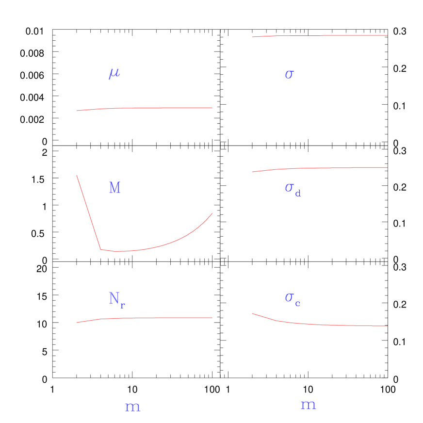
Inserting $n_{s}=1.13$ and $dn_{s}/d\ln k=-0.055$ on the comoving scale $k_{0}=0.002\,{\rm Mpc}^{-1}$ obtained by WMAPext+2dFGRS+Ly$\alpha$ Peiris , we can obtain the values of all parameters for each $m$. For example, in the case $m=2$, $\mu=2.7\times 10^{-3}=6.5\times 10^{15}$ GeV, $M=1.6,\sigma=0.28$, and $\sigma_{d}=0.24$. The number of $e$-folds, $N_{r}$, of smooth hybrid inflation after the scale with the desired spectral shape has crossed the Hubble radius is found to be 10. Also, in the case of $m=8$, $\mu=2.9\times 10^{-3}=7.0\times 10^{15}$ GeV, $M=0.14,\sigma=0.28,\sigma_{d}=0.25$, and $N_{r}=11$. The values of parameters for each $m$ is depicted in Fig. 1. Note that even if we take large $m$, $N_{r}$ does not increase in proportion to $m^{2/3}$, because an increase in $m$ is accompanied by that in $M$ as long as we use the observed values of $n_{s},~{}dn_{s}/d\ln k$, and ${\cal R}$. As a result $N_{r}$ does not change significantly no matter how large $m$ may be, as seen in Fig. 1. Therefore, another inflation is necessary in order that the scale with the desired spectral shape be pushed to the comoving scale $k_{0}=0.002\,{\rm Mpc}^{-1}$.

III Smooth hybrid new inflation in supergravity

As the second inflation to follow smooth hybrid inflation, we adopt new inflation proposed by Izawa and Yanagida IY . While hybrid inflation including smooth hybrid inflation predicts a high reheating temperature because the inflaton has gauge couplings and its energy scale is relatively high usually, new inflation predicts a sufficiently low reheating temperature to avoid overproduction of gravitinos. Thus, the occurrence of new inflation following smooth hybrid inflation is favorable also in this respect. Furthermore, in our model, the initial value of new inflation is dynamically set during smooth hybrid inflation, which evades the severe initial value problem of new inflation. In this section, after reviewing new inflation briefly, we discuss smooth hybrid new inflation in supergravity by considering full superpotential and Kähler potential.

The superpotential of new inflation is given by

$$W_{N}[\Phi]=v^{2}\Phi-\frac{g}{n+1}\Phi^{n+1},$$ (17)

where we introduce a chiral superfield $\Phi$ with an $R$ charge $2/(n+1)$, but assume that the U$(1)_{R}$ symmetry is dynamically broken to a discrete $Z_{2n~{}R}$ symmetry at a scale $v\ll\mu$. Here $g$ is a coupling constant of order of unity and we also assume that both $g$ and $v$ are real and positive for simplicity. We assume $n$ is larger than 2 because $g$ must be unnaturally small to realize inflation if $n=2$. The $R$-invariant Kähler potential is given by

$$K_{N}=|\Phi|^{2}+\frac{c_{N}}{4}|\Phi|^{4}+\cdots,$$ (18)

where $c_{N}$ is a constant smaller than unity.

From Eqs. (17) and (18), the scalar potential of new inflaton reads

$$V_{N}[\Phi] = \frac{\exp\left(|\Phi|^{2}+\frac{c_{N}}{4}|\Phi|^{4}\right)}{1+c_{N}|\Phi|^{2}}$$ (19)

$$\times\left[~{}\left|\left(1+|\Phi|^{2}+\frac{c_{N}}{2}|\Phi|^{4}\right)v^{2}-\left(1+\frac{|\Phi|^{2}}{n+1}+\frac{c_{N}|\Phi|^{4}}{2(n+1)}\right)g\Phi^{n}\right|^{2}\right.$$

$$~{}~{}~{}\left.-3\left(1+c_{N}|\Phi|^{2}\right)|\Phi|^{2}\left|v^{2}-\frac{g}{n+1}\Phi^{n}\right|^{2}\right].$$

It has a minimum at

$$|\Phi|_{\min}\cong\left(\frac{v^{2}}{g}\right)^{\frac{1}{n}}~{}~{}~{}{\rm and~{}~{}Im}\Phi^{n}_{\min}=0,$$ (20)

with a negative energy density

$$V_{N}[\Phi_{\min}]\cong-3e^{K_{N}}|W_{N}[\Phi_{\min}]|^{2}\cong-3\left(\frac{n}{n+1}\right)^{2}v^{4}|\Phi_{\min}|^{2}.$$ (21)

As was done in IY , we assume that this negative energy density is canceled by a positive contribution coming from supersymmetry breaking, $\Lambda_{\rm SUSY}^{4}$, which relates energy scale $v$ of this model with the gravitino mass $m_{3/2}$ as

$$m_{3/2}\cong\frac{n}{n+1}\left(\frac{v^{2}}{g}\right)^{\frac{1}{n}}v^{2}.$$ (22)

Then, the potential of new inflaton is approximated as

$$V_{N}[\phi]\cong v^{4}-\frac{c_{N}}{2}v^{4}\phi^{2}-\frac{2g}{2^{n/2}}v^{2}\phi^{n}+\frac{g^{2}}{2^{n}}\phi^{2n},$$ (23)

where we identified the real part of $\Phi$ with the inflaton $\phi\equiv\sqrt{2}\,\rm{Re}\,\Phi$. The derivative of the effective potential is given by

$$\frac{dV_{N}}{d\phi}\cong-c_{N}v^{4}\phi-{2^{\frac{2-n}{2}}}{ngv^{2}}\phi^{n-1}+2^{1-n}ng^{2}\phi^{2n-1}.$$ (24)

Since the last term is negligible during inflation, the dynamics is determined by the first term for $\phi<\phi_{d}$ and the second term for $\phi>\phi_{d}$ with

$$\phi_{d}\equiv\sqrt{2}\left(\frac{c_{N}v^{2}}{gn}\right)^{\frac{1}{n-2}}.$$ (25)

Then, the slow-roll parameters are given by

$$\epsilon_{N}\cong\frac{1}{2}\left(c_{N}\phi+{2^{\frac{2-n}{2}}}{ng}\frac{\phi^{n-1}}{v^{2}}\right)^{2},~{}~{}~{}\eta_{N}=-c_{N}-{2^{\frac{2-n}{2}}}{n(n-1)g}\frac{\phi^{n-2}}{v^{2}}.$$ (26)

Thus inflation is realized for $c_{N}\ll 1$ and ends at $\phi=\phi_{c}$ defined as

$$\phi_{c}\equiv\sqrt{2}\left(\frac{(1-c_{N})v^{2}}{gn(n-1)}\right)^{\frac{1}{n-2}},$$ (27)

when $|\eta|$ becomes as large as unity.

The total number of $e$-folds of new inflation is estimated as

$$N_{N}=-\int_{\phi_{i}}^{\phi_{c}}d\phi\frac{V_{N}}{dV_{N}/d\phi}\cong\int_{\phi_{i}}^{\phi_{d}}d\phi\frac{d\phi}{c_{N}\phi}+\int_{\phi_{d}}^{\phi_{c}}\frac{2^{\frac{n-2}{2}}v^{2}}{gn\phi^{n-1}}=\frac{1}{c_{N}}\ln\frac{\phi_{d}}{\phi_{i}}+\frac{1-nc_{N}}{(n-2)c_{N}(1-c_{N})}$$ (28)

for $0<c_{N}<n^{-1}$. If $c_{N}$ vanishes, we instead find

$$N_{N}=\int_{\phi_{i}}^{\phi_{c}}d\phi\frac{2^{\frac{n-2}{2}}v^{2}}{gn\phi^{n-1}}=\frac{2^{\frac{n-2}{2}}v^{2}}{gn(n-2)}\phi_{i}^{2-n}-\frac{n-1}{n-2}.$$ (29)

Here $\phi_{i}$ is the initial value of $\phi$, which is set dynamically during smooth hybrid inflation, as shown below.

We investigate full dynamics of smooth hybrid new inflation by assuming that there are no direct interactions between fields relevant to hybrid inflation discussed in the previous section and $\Phi$. That is, the full superpotential and Kähler potential is given by $W=W_{H}+W_{N}$ and $K=K_{H}+K_{N}$.

In the hybrid inflation stage $\sigma>\sigma_{c}$, the cosmic energy density is dominated by the false vacuum energy $\mu^{4}$, which gives the interaction terms between $S$ and $\Phi$:

$$V\supset\mu^{4}|\Phi|^{2}+\mu^{2}v^{2}(\Phi^{\ast}S+\Phi S^{\ast})+\cdots=\frac{1}{2}\mu^{4}(\phi^{2}+\chi^{2})+\mu^{2}v^{2}\sigma\phi+\cdots.$$ (30)

Hence at the end of hybrid inflation, $\sigma=\sigma_{c}$, $\phi$ and $\chi\equiv\sqrt{2}\,\rm{Im}\,\Phi$ have a minimum at

$$\phi_{\min}\cong-\frac{v^{2}}{\mu^{2}}\sigma_{c}=-5^{\frac{1}{6}}\left(\frac{2}{3}\right)^{\frac{1}{2}}\frac{v^{2}}{\mu^{2}}(\mu M)^{\frac{1}{3}},~{}~{}~{}~{}~{}~{}\chi_{\min}\cong 0,$$ (31)

respectively. Here and hereafter we set $m=2$ for definiteness.

Since the effective mass is larger than the Hubble parameter during hybrid inflation, the above configuration is realized with the dispersion

$$\langle(\phi-\phi_{\min})^{2}\rangle=\langle\chi^{2}\rangle=\frac{3}{8\pi^{2}}\frac{H_{H}^{4}}{\mu^{4}}=\frac{\mu^{4}}{24\pi^{2}},$$ (32)

due to quantum fluctuations BD , where $H_{H}\equiv\mu^{2}/\sqrt{3}$ is the Hubble parameter during smooth hybrid inflation. The ratio of quantum fluctuation to the expectation value should satisfy

$$\frac{\sqrt{\langle(\phi-\phi_{\min})^{2}\rangle}}{|\phi_{\min}|}=\frac{1}{4\times 5^{\frac{1}{6}}\pi}\left(\frac{\mu^{5}}{M}\right)^{\frac{1}{3}}\left(\frac{\mu}{v}\right)^{2}\ll 1,$$ (33)

so that the initial value of the inflaton for new inflation is located off the origin with an appropriate magnitude.

After $\sigma$ reaches $\sigma_{c}$, smooth hybrid inflation ends and the fields $S$ and $\Psi(\overline{\Psi})$ start oscillating and decay eventually. If this oscillation phase lasts for a prolonged period due to gravitationally suppressed interactions of these fields, $\phi$ will also oscillate and its amplitude decreases with an extra factor $v/\mu$ Kawasaki:1998vx . In this case, new inflation could start with an even smaller value of $\phi$ depending on its phase of oscillation at the onset of inflation (see Kanazawa:1999ag for an analytic estimate of the initial phase). So we set the initial value of $\phi$ as

$$\phi_{i}=\left(\frac{v}{\mu}\right)\phi_{\min},$$ (34)

and new inflation occurs until $\phi=\phi_{c}$ with the potential (23).

Contrary to the smooth hybrid inflation regime we do not have much precise observational constraints on the new inflation regime, so we cannot fully specify values of the model parameters for new inflation. Hence let us content ourselves with a few specific examples. First we consider the cases with $c_{N}=0$. Then from Eq. (29) the number of $e$-folds of new inflation reads

$$N_{N}=\frac{2^{\frac{n-2}{2}}v^{2}}{gn(n-2)}\phi_{i}^{2-n}-\frac{n-1}{n-2}\cong\frac{2^{\frac{n-2}{2}}v^{2}}{gn(n-2)}\phi_{i}^{2-n}.$$ (35)

This should be around $40+(2/3)\ln(\mu/v)$ to push the comoving scale with appropriate spectral shape to the appropriate physical length scale. On the other hand, the amplitude of curvature perturbation at the onset of new inflation, $\phi=\phi_{i}$, is given by

$${\cal R}=\frac{n-2}{2\sqrt{3}\pi}N_{N}\frac{\mu^{3}}{v\sigma_{c}}\cong 1.5\times 10^{-4}(n-2)\frac{\mu}{v}\frac{N_{N}}{40},$$ (36)

where use has been made of the values $\mu=2.7\times 10^{-3}$ and $\sigma_{c}=0.17$ in the last equality. From Eq. (28) we find

$$v = 9.4\times 10^{-5}\left(\frac{gN_{N}}{40}\right)^{-\frac{1}{4}},~{}~{}~{}{\rm for}~{}n=4,$$

$$v = 9.6\times 10^{-4}\left(\frac{gN_{N}}{40}\right)^{-\frac{1}{10}},~{}~{}~{}{\rm for}~{}n=6,$$

$$v = 1.8\times 10^{-3}\left(\frac{gN_{N}}{40}\right)^{-\frac{1}{16}},~{}~{}~{}{\rm for}~{}n=8,$$

$$v = 2.3\times 10^{-3}\left(\frac{gN_{N}}{40}\right)^{-\frac{1}{22}},~{}~{}~{}{\rm for}~{}n=10,$$

$$v = 2.7\times 10^{-3}\left(\frac{gN_{N}}{40}\right)^{-\frac{1}{28}},~{}~{}~{}{\rm for}~{}n=12.$$ (37)

For $g<1$ and $n\geq 12$, $v$ is larger than $\mu$, which contradicts with our assumption that new inflation takes place after hybrid inflation at lower energy scale. Setting $g=1$, we find for $n=4$ that ${\cal R}\cong 8.7\times 10^{-3}$ at the onset of new inflation which corresponds to the comoving scale $\ell_{*}\sim 1.3$ Mpc today. $v$ can be close to $\mu$ and ${\cal R}$ can be smaller only for $g\lesssim 10^{-6}$, which is quite unnatural. For $n=8$, we find that ${\cal R}\cong 1.4\times 10^{-3}$ at the onset of new inflation which corresponds to the comoving scale $\ell_{*}\sim 190$ kpc today. These fluctuations cause the early formation of dark halo objects with comoving scale $\ell_{*}$. In the above cases, since $\ell_{*}$ is larger than about 1 kpc, the dark halos may cause a cosmological problem because they significantly harm subsequent galaxy formation or produce too many gravitational lens events.

On the other hand, for $c_{N}\neq 0$, we find

$${\cal R}=\frac{\mu^{2}}{2\sqrt{3}\pi c_{N}\sigma_{c}}\frac{\mu}{v}\cong 3.8\times 10^{-6}c_{N}^{-1}\frac{\mu}{v},$$ (38)

at the onset of new inflation. It is independent on $n$ and $g$. From Eq. (28), $v$ is related to the number of $e$-folds $N_{N}$:

$$v=\left[\frac{\sigma_{c}}{\sqrt{2}\mu^{3}}\left(\frac{c_{N}}{ng}\right)^{-\frac{1}{n-2}}\exp{\left\{c_{N}\left(N_{N}-\frac{1-nc_{N}}{(n-2)c_{N}(1-c_{N})}\right)\right\}}\right]^{\frac{n-2}{8-3n}}.$$ (39)

Thus, if we take $c_{N}=0.1$, for example, $N_{N}=40$ implies

$$v = 2.5\times 10^{-5}g^{-\frac{1}{4}},~{}~{}~{}{\rm for}~{}n=4,$$

$$v = 2.7\times 10^{-4}g^{-\frac{1}{10}},~{}~{}~{}{\rm for}~{}n=6,$$

$$v = 4.8\times 10^{-4}g^{-\frac{1}{16}},~{}~{}~{}{\rm for}~{}n=8,$$

$$v = 6.4\times 10^{-4}g^{-\frac{1}{22}},~{}~{}~{}{\rm for}~{}n=10.$$ (40)

For $n=4$, ${\cal R}\cong 4.1\times 10^{-3}g^{1/4}$ at the comoving scale $\ell_{*}\cong 3.1g^{1/6}$ Mpc, which again causes the dark halo problem unless $g$ is extremely small. On the other hand, for $n\geq 6$ and $g=1$, ${\cal R}\lesssim 3.8\times 10^{-4}$ at the comoving scale $\ell_{*}\lesssim 650$ kpc, which may be helpful for early star formation which is required for early re-ionization Bennett and from the age estimate of high-redshift quasars using the cosmological chemical clock jy .

IV Discussion and Conclusion

In this paper we proposed a new model of inflation in supergravity, in which the two new features discovered by the recent precision measurements of cosmic microwave background anisotropy can be explained simultaneously and naturally: namely, the running of spectral index of density fluctuations on large scale as preferred by the first-year WMAP data and a large enough amplitude of fluctuation on small scale relevant to first star formation to realize early re-ionization as discovered by WMAP. The desired running feature–that is, the spectral index with $n_{s}>1$ on a large scale and $n_{s}<1$ on a smaller scale–is naturally generated by the balance between the nonrenormalizable term in the superpotential and supergravity effects without resorting to the one-loop effect contrary to our previous models YY ; KYY .

Compared with the chaotic hybrid new inflation model in supergravity YY , the present model has somewhat simpler symmetry structures, although we have been unable to explain the hierarchy of the energy scales of two inflations here unlike in the previous model YY . Because our previous model induces string formation with a fairly large energy scale, if forthcoming analysis could rule out such topological defects, the present model would be the only surviving model among the two.

Figure 1: The values of all parameters are shown for each $m$.