Axino Dark Matter and the CMSSM

Abstract:

If the axino is the lightest superpartner and satisfies cosmological bounds, including a preferred range of the relic abundance of cold dark matter, then the usual stringent constraints on the parameter space of the CMSSM become greatly relaxed. The lightest superpartner of the usual CMSSM spectrum will appear to be stable in collider experiments but will not necessarily obey relic abundance constraints. It may be either neutral (lightest neutralino) or charged (typically a stau). With the axino as cold dark matter, large regions of the CMSSM, often corresponding to heavy superpartners, become allowed, depending on the axino mass and the reheating temperature.

1 Introduction

The lightest supersymmetric particle (LSP) that arises in models featuring supersymmetry (SUSY) at low energy with the conservation of $R$–parity can be a cold dark matter (DM) candidate [1]. The requirement that the LSP is neutral and produced in the required abundance in the early Universe sets strong constraints on the minimal supersymmetric standard model (MSSM) [1] or its constrained version (CMSSM) [2]. In the CMSSM, the LSP is often the lightest neutralino with a large bino component [3, 4, 5]. In particular, the cases of a neutralino nearly degenerate with the lighter stau [6] or stop [7] are often of cosmological importance, but parameter choices for which such charged particles themselves are the LSP are thought to be excluded on astrophysical grounds. In fact, very strong bounds on the presence of electrically charged and colored relics have been obtained using the unsuccessful searches for exotic nuclei: strong bounds on electrically charged relics have been obtained up to masses of the order $10^{8}$ GeV, while masses greater than a few  TeV for colored thermal relics remain consistent with observation [8].

However, if the LSP does not belong to the usual MSSM spectrum, other possibilities arise. One such attractive scenario involves supersymmetric models implementing the Peccei–Quinn mechanism for solving the strong CP problem [9]. In this class of models the axino, the fermionic superpartner of the axion, can naturally be the LSP and constitute the dominant component of DM in the form of warm [10, 11, 12, 13, 14] or cold dark matter (CDM) [15, 13, 16]. (See also [17, 18].) This is because, unlike for the neutralino, the mass of the axino is not directly determined by the soft SUSY–breaking terms and can be much smaller [19].

Axinos can be efficiently produced in the early Universe through several possible processes. A class of thermal production (TP) processes involves scatterings and decays of particles in the primordial plasma. Alternatively, in non–thermal production (NTP) the next–to–lightest supersymmetric particle (NLSP) decays after first freezing out from the plasma. In addition, one can think of other possible production mechanisms, e.g. from inflaton decay, but they are much more model dependent and not necessarily as efficient. The above processes are supposed to re–generate the axinos, after their primordial population has been diluted as a result of inflation and subsequent reheating with $T_{\rm R}\mathrel{\hbox to0.0pt{\lower 4.0pt\hbox{\hskip 1.0pt$\sim$}\hss}\raise 1.0pt\hbox{$<$}}f_{a}$ (with $f_{a}\sim 10^{11}\,\mbox{GeV}$ being the Peccei–Quinn scale) in order to avoid overclosure. Otherwise, the axinos would have to be very light, $m_{\tilde{a}}<0.2\,\mbox{keV}$ [12], with an update in [13], thus constituting warm DM.

In [15, 13, 16] we conducted a detailed investigation of the axino LSP as CDM in the KSVZ–type (hadronic) axion models [20] coupled with the MSSM. As summarized in Figs. 8 and 9 of [16], we showed that, for $m_{\tilde{a}}\mathrel{\hbox to0.0pt{\lower 4.0pt\hbox{\hskip 1.0pt$\sim$}\hss}\raise 1.0pt\hbox{$>$}}100\,\mbox{keV}$ and $T_{\rm R}\mathrel{\hbox to0.0pt{\lower 4.0pt\hbox{\hskip 1.0pt$\sim$}\hss}\raise 1.0pt\hbox{$<$}}5\times 10^{6}\,\mbox{GeV}$, the axino can constitute cold DM, while at a lower mass range and larger $T_{\rm R}$ it could be a warm or even hot DM relic. At $T_{\rm R}\mathrel{\hbox to0.0pt{\lower 4.0pt\hbox{\hskip 1.0pt$\sim$}\hss}\raise 1.0pt\hbox{$>$}}10^{4}\,\mbox{GeV}$ NTP is typically subdominant while TP processes allows for a narrow region of $m_{\tilde{a}}$ to satisfy the relic abundance constraint $\Omega_{\tilde{a}}h^{2}\sim 1$. On the other hand, in the region of $m_{\tilde{a}}\mathrel{\hbox to0.0pt{\lower 4.0pt\hbox{\hskip 1.0pt$\sim$}\hss}\raise 1.0pt\hbox{$>$}}10\,\mbox{MeV}$ and $T_{\rm R}\mathrel{\hbox to0.0pt{\lower 4.0pt\hbox{\hskip 1.0pt$\sim$}\hss}\raise 1.0pt\hbox{$<$}}10^{4}\,\mbox{GeV}$, the NTP mechanism of neutralino (or other NLSP) decay after freeze-out often plays a dominant role in producing enough axinos, while at larger $T_{\rm R}$ TP does this too efficiently. Contrary to the case of a gravitino, the other popular alternative SUSY candidate for the LSP and CDM, the lifetime of the NLSP is much shorter than $10^{4}\sec$ and therefore avoids the very strong bound coming from photo–destruction of light elements after nucleosynthesis. For this reason, only the much weaker constraints from hadronic showers play a role for the axino LSP scenario. However, if the squarks are much lighter than the gluino, their decays in TP processes can reduce an upper bound on $T_{\rm R}$ further [16].

In this paper, we turn our attention to investigating the implications on the allowed spectra of the CMSSM of assuming the axino as the LSP and CDM, with the right amount of the cosmological relic abundance and with other constraints, especially from nucleosynthesis, satisfied. This is of interest because the standard paradigm is highly constrained, especially at not too large values of $\tan\beta$ on which we will concentrate here. While this makes the CMSSM highly predictive, a question arises as to whether viable alternative scenarios exist which would lead to very different predictions and to possibly relaxing the stringent cosmological bounds on the CMSSM without abandoning a supersymmetric explanation for CDM.

As we will see, very different regions of the CMSSM parameter space will often become allowed. In particular, it will be possible to have either an electrically neutral NLSP (the lightest neutralino) or a charged one (the lighter stau). The NLSP will appear in a collider detector as a stable lightest ordinary supersymmetric partner (LOSP). Since axino couplings are suppressed by the Peccei–Quinn scale, the NLSP lifetime is long compared to the timescales of relevance for accelerator searches. Therefore, the usual mass bounds arising from the decay of the sparticle into the lightest neutralino are not applicable. Depending of the case of a chargino or slepton L(O)SP, the bounds become a bit relaxed or more stringent. For the case of a “stable” charged L(O)SP, a general lower bound of about $99.4\,\mbox{GeV}$ has been obtained at LEP [21]. This may, once superpartners are discovered at the LHC, allow one to distinguish the case of the axino from the usually assumed case of the lightest neutralino as the true LSP.

In this context it might be worth commenting on the gravitino as the LSP and CDM. In a recent study [22] it has been concluded that one can find limited regions of the CMSSM where the gravitino LSP would be allowed but that, in these regions, NLSP decays typically provide too little relic abundance for the gravitino to fall into the favored range, if one does not want to spoil nucleosynthesis predictions. However, thermal production processes involving gluino decay and scattering may rectify this [23].

In the following, we will first summarize the effective axino–neutralino couplings and compute effective axino–stau couplings and corresponding NLSP lifetimes in the MSSM coupled with the KSVZ axion models. We will then discuss bounds on the NLSP number density from primordial nucleosynthesis constraints and summarize the calculation of axino relic abundance. We will next concentrate on the CMSSM and will first illustrate the cosmologically allowed parameter space in the CMSSM in the standard scenario with the neutralino LSP. Next we will re–compute the relic abundance in the CMSSM with the axino as the LSP and will investigate the resulting changes in the cosmological bounds on the ($m_{1/2},m_{0}$) plane for several values of the axino mass and $T_{\rm R}$.

2 The Axion Multiplet Interactions

In the Peccei–Quinn (PQ) solution to the strong CP problem, a complex scalar field is used to break the global $U(1)_{PQ}$ at a high scale $f_{a}\sim 10^{11}\,\mbox{GeV}$. Its Goldstone boson component, the axion, plays the role of a dynamical field $\theta_{QCD}$ and relaxes at the origin after the QCD phase transition [24, 25]. After chiral symmetry breaking, the axion acquires a tiny mass from instanton effects [26]. As before, in this work we concentrate on the KSVZ–type axion type of interactions [20]. In the DFSZ case [27] in general the mixing between the axino and the neutralinos can become substantial and enhance the couplings discussed here.

In the context of supersymmetry the axion field becomes a chiral multiplet [28] which contains not only the pseudoscalar axion and the scalar saxion with $R$–parity $+1$, but also one $R=-1$ state, their fermionic superpartner, the axino $\tilde{a}$. The interaction of the axino with gluons and gluinos proceeds via diagrams that are the supersymmetric analogues of the fermionic triangle anomaly diagrams for the heavy states $Q$. After integrating out the heavy KSVZ quarks $Q$ and squarks $\widetilde{Q}$, where $m_{Q,\widetilde{Q}}\sim f_{a}$, there arises an effective dimension–5 interaction term

$${\cal L}_{\tilde{a}g\tilde{g}}=\frac{\alpha_{s}}{8\pi(f_{a}/N)}\bar{\tilde{a}}\gamma_{5}\sigma^{\mu\nu}\tilde{g}^{b}G^{b}_{\mu\nu}$$ (1)

where $b=1,\ldots,8$, $\tilde{g}$ is the gluino and $G$ is the strength of the gluon field, while $N$ is the number of flavors of quarks with the Peccei–Quinn charge, and is equal to $1$ ($6$) in KSVZ (DFSZ) models. For the remainder of this paper, we understand $f_{a}$ to mean $f_{a}/N$.

The coupling (1) and the corresponding axion coupling can also be written in a supersymmetric form as a Wess–Zumino term in the MSSM superpotential

$$W_{WZ}={\alpha_{s}\over 2\sqrt{2}\pi f_{a}}{\cal A}\;Tr\left[W_{\alpha}W^{\alpha}\right],$$ (2)

where ${\cal A}$ is the axion chiral multiplet, $W_{\alpha}$ the vector multiplet containing the gluon, and the trace sums over color indices. An interesting feature is that the coupling above is only determined by the QCD anomaly of the heavy states and is not subject to renormalization [29] or model dependence.

In an analogous way, Wess–Zumino terms can arise also for other gauge interactions, depending on the charge of the heavy quark multiplet. At high energies, where all leptons can be considered massless, such interactions can be rotated into the $U(1)_{Y}$ direction [13] and we are left to consider only the term

$$W_{WZ}={\alpha_{Y}C_{aYY}\over 4\sqrt{2}\pi f_{a}}{\cal A}\;B_{\alpha}B^{\alpha},$$ (3)

where $B_{\alpha}$ is the hypercharge vector multiplet and $C_{aYY}$ is a model–dependent factor [30], which vanishes if the heavy KSVZ quarks are electrically neutral. If they have electric charge $e_{Q}=-1/3,+2/3$, then $C_{aYY}=2/3,8/3$. This superpotential term leads to the addition of the following effective dimension–5 interaction term to the low–energy Lagrangian

$${\cal L}_{\tilde{a}B\widetilde{B}}=\frac{\alpha_{Y}C_{aYY}}{8\pi f_{a}}\bar{\tilde{a}}\gamma_{5}\sigma^{\mu\nu}\widetilde{B}B_{\mu\nu}$$ (4)

Cosmological implications of the effective axino–gauge boson–gaugino operators (1) and  (4) have been extensively studied in [13].

However, in addition to the above interactions, there is also an effective dimension–4 coupling of the axino to fermions and sfermions [16]

$${\cal L}_{\tilde{a}\psi\widetilde{\psi}}=\Sigma_{j}\,\,g_{{\rm eff},\,j}^{L/R}\;\widetilde{\psi}^{L/R}_{j}\,\bar{\psi}_{j}P_{R/L}\gamma_{5}\tilde{a},$$ (5)

where $\psi_{j}$ and $\widetilde{\psi}_{j}$ can be any of the SM fermions and their superpartners. This effective coupling, which arises at two–loop level in KSVZ models (and therefore at a one–loop level in the effective theory valid much below $f_{a}$), is the dominant channel for inducing the decay of charged NLSPs to axinos.

The effective vertex in (5) and its effect on the axino abundance was computed in the case of light quarks in [16] where it was found that the dominant contribution was due to the logarithmically divergent part of the gluon–gluino–quark loop and was proportional to the gluino mass $m_{\tilde{g}}$,

$$g_{{\rm eff},\,q}^{L/R}\simeq\mp{\alpha_{s}^{2}\over\sqrt{2}\pi^{2}}{m_{\tilde{g}}\over f_{a}}\log\left({f_{a}\over m_{\tilde{g}}}\right).$$ (6)

Here the quark mass has been neglected. This result was obtained in the low energy effective theory given by the MSSM plus the interaction in (1), i.e. from the one–loop diagrams as in Fig. 1, where the Peccei–Quinn scale $f_{a}$ was used as a cut–off in the loop momentum integral. This procedure is justified by the fact that the effective theory is valid only below the scale and in practice amounts to absorbing our ignorance about the high energy theory into the parameter $f_{a}$. In this way a model–independent computation of the effective coupling was performed. (Integrating the Renormalization Group Equation for the effective coupling above between $f_{a}$ and $m_{\tilde{g}}$ with vanishing boundary condition, gives very similar results.) Adopting the same strategy as in [16], here we extend the computation of the effective vertex to the case of the tau–stau–axino, including the effects of the tau mass.

Note that the procedure above gives the dominant coupling of the axino to the sfermions as long as the mixing of the axino with the other neutralinos is negligible. In the DFSZ case, this is not the case and therefore the computation of the production of axinos in the thermal bath is more involved. For what concerns NTP instead, the picture is similar, apart from shorter NLSP lifetimes [31].

Figure 1: The Feynman diagrams contributing to the squark–quark–axino interaction. The thick dot denotes the effective gluino–gluon–axino vertex.

3 The Lighter Stau as the NLSP

In order to study the charged NLSP scenario in the CMSSM, first we evaluate the effective couplings between the lighter stau and the axino.

3.1 An Effective Stau–Tau–Axino Coupling

As shown in Fig. 2, the stau couples to an axino and a tau via triangle diagrams analogous to those giving rise to the squark–quark–axino coupling. The effective axino–gauge boson–neutralino vertex in this diagram, represented by a thick dot, is given by (4).

Figure 2: The Feynman diagrams giving the dominant contribution to the stau–tau–axino coupling.

In the following we present the result for the loop integration. We keep only the dominant contribution and regulate its logarithmic divergence with the cut–off $f_{a}$, in the spirit of [16].

Consider first the loop containing a photon. This diagram gives rise to the following effective vertex involving an axino $\tilde{a}$ with momentum $k_{1}$, a tau $\tau$ with momentum $k_{2}$ and a stau $\tilde{\tau}_{R/L}$ with momentum $k_{1}+k_{2}$,

$$i\bar{u}_{\tau}(k_{2})(G^{\gamma}_{L/R}(k_{1},k_{2})P_{L/R}+\widetilde{G}^{\gamma}_{R/L}(k_{1},k_{2})P_{R/L})\gamma_{5}v_{\tilde{a}}(k_{1})$$ (7)

The “gauge” couplings $G^{\gamma}_{L/R}$ are as follows

$$G^{\gamma}_{L} \simeq -\sum_{i=1}^{4}{3\sqrt{2}\alpha_{em}^{2}\over 8\pi^{2}}\left({C_{aYY}Z_{1i}Z_{i1}\over\cos^{2}\theta_{W}}\right)\left({m_{\chi_{i}}\over f_{a}}\right)\log\left({f_{a}\over m_{\chi_{i}}}\right)$$ (8)

$$G^{\gamma}_{R} \simeq +\sum_{i=1}^{4}{3\sqrt{2}\alpha_{em}^{2}\over 16\pi^{2}}\left({C_{aYY}Z_{1i}\over\cos^{2}\theta_{W}}\right)\left(Z_{i1}+{Z_{i2}\over\tan\theta_{W}}\right)\left({m_{\chi_{i}}\over f_{a}}\right)\log\left({f_{a}\over m_{\chi_{i}}}\right),$$ (9)

where $i=1,\ldots,4$ denotes the four neutralino species and $Z_{ij}$ is the matrix that changes basis to the neutralino mass eigenstates.

The “Yukawa” couplings $\widetilde{G}_{R/L}$ arise due to the higgsino content of the intermediate neutralino and are given by

$$\widetilde{G}^{\gamma}_{R/L}\simeq-\sum_{i=1}^{4}{3\sqrt{2}\alpha_{em}^{2}\over 8\pi^{2}}\left({C_{aYY}Z_{1i}}\over{\cos^{2}\theta_{W}}\right)\left({Z_{i3}m_{\tau}\over 2m_{W}\tan\theta_{W}\cos\beta}\right)\left({m_{\chi_{i}}\over f_{a}}\right)\log\left({f_{a}\over m_{\chi_{i}}}\right).$$ (10)

The analogues of these $P_{R/L}$ couplings were not considered in the case of the squark–quark–axino coupling in [16] because the dominant diagrams there involved an internal gluino instead of the neutralino.

In the calculation of $\widetilde{G}^{\gamma}_{R/L}$, $m_{\tau}$ appears in the stau–tau–neutralino coupling but has been neglected in the propagator and in the final state mass. This is justified because the dominant scales in the loop and the kinematics, respectively $m_{\chi}$ and $m_{\tilde{\tau}}$, are both much larger than $m_{\tau}$. Moreover, since $m_{\tau}/m_{W}\simeq 0.02$ and $Z_{1i}$ and $Z_{i3}$ cannot both be close to $1$, we conclude that the effect of the tau mass is small also in the coupling and that $\widetilde{G}^{\gamma}_{R/L}$ can safely be neglected, as long as we assume $\tan\beta<50$.

We turn now to the loop containing a $Z$–boson instead of a photon. The dominant contribution to the loop integral comes from the high energy scale $f_{a}$, and is the same for both loops. In fact, adding a $Z$–boson mass term to the denominator leads to a suppression relative to the photon case of only a few percent, which we neglect. Therefore, the only difference with respect to the photon loop is in the couplings of the $Z$–boson to the tau, and to the neutralino and the axino. Note also that the $\widetilde{G}^{Z}_{R/L}$ couplings are suppressed in the same way as the corresponding $\widetilde{G}^{\gamma}_{R/L}$ and therefore will be neglected.

In summary, the two loop diagrams together lead to the following effective $\tilde{\tau}_{R/L}-\tau-\tilde{a}$ couplings

$$G_{L} \simeq -\sum_{i=1}^{4}{3\sqrt{2}\alpha_{em}^{2}\over 8\pi^{2}}\left({C_{aYY}Z_{1i}Z_{i1}\over\cos^{2}\theta_{W}}\right)\left(1-\tan^{2}\theta_{W}\right)\left({m_{\chi_{i}}\over f_{a}}\right)\log\left({f_{a}\over m_{\chi_{i}}}\right)$$ (11)

$$G_{R} \simeq +\sum_{i=1}^{4}{3\sqrt{2}\alpha_{em}^{2}\over 16\pi^{2}}\left({C_{aYY}Z_{1i}\over\cos^{2}\theta_{W}}\right)\left({3\over 2}-{1\over 2}\tan^{2}\theta_{W}\right)$$ (12)

$$\times\left(Z_{i1}+{Z_{i2}\over\tan\theta_{W}}\right)\left({m_{\chi_{i}}\over f_{a}}\right)\log\left({f_{a}\over m_{\chi_{i}}}\right).$$

In general, the NLSP is a linear combination of the two staus, $\tilde{\tau}_{1}=\cos\theta_{\tilde{\tau}}\,\tilde{\tau}_{L}+\sin\theta_{\tilde{\tau}}\,\tilde{\tau}_{R}$. Therefore, the photon loop leads to the following effective $\tilde{\tau}_{1}-\tau-\tilde{a}$ coupling

$$i\bar{u}_{\tau}(k_{1})\left[\sin\theta_{\tilde{\tau}}\,G_{L}(k_{1},k_{2})P_{L}+\cos\theta_{\tilde{\tau}}\,G_{R}(k_{1},k_{2})P_{R}\right]\gamma_{5}v_{\tilde{a}}(k_{1})$$ (13)

In the following, we consider the consequences of this effective vertex for the stau decay.

3.2 Light Stau Decay

Through the effective vertex described above, a $\tilde{\tau}_{1}$ can decay into an axino and a tau, with a width

$$\Gamma_{{\tilde{\tau}}_{1}\rightarrow\,\tilde{a}\,\tau}\simeq\frac{m_{{\tilde{\tau}}_{1}}}{16\pi}\left(\sin^{2}\theta_{\tilde{\tau}}|\,G_{L}|^{2}+\cos^{2}\theta_{\tilde{\tau}}|\,G_{R}|^{2}\right).$$ (14)

In order to get a rough estimate of the decay rate without considering the whole neutralino sector, note that the two couplings contain the terms $Z_{1i}m_{\chi_{i}}Z_{i1}$ and $Z_{1i}m_{\chi_{i}}Z_{i2}$. The quantity $\Sigma_{i}\,Z_{1i}m_{\chi_{i}}Z_{i1}$ is simply $M_{11}$ of the undiagonalized neutralino mass matrix in the flavor basis, which is just $M_{1}$. Similarly, $\Sigma_{i}\,Z_{1i}m_{\chi_{i}}Z_{i2}$ is $M_{12}$, which is zero. In the expressions for $G_{L}$ and $G_{R}$ above, these sums are modified slightly by the logarithmic factors, but as a rough estimate we can assume that they do not modify strongly the cancellation and ignore the $Z_{i2}$ term in $G_{R}$. Then we have

$$G_{R}\sim-{G_{L}\over 4}\frac{3-\tan^{2}\theta_{W}}{1-\tan^{2}\theta_{W}}\simeq-0.96\,G_{L}$$ (15)

and so

$$\Gamma_{{\tilde{\tau}}_{1}\rightarrow\,\tilde{a}\,\tau} \sim \frac{m_{{\tilde{\tau}}_{1}}}{16\pi}(G_{L})^{2}(1-0.069\cos^{2}\theta_{\tilde{\tau}})$$ (16)

$$\sim \frac{m_{{\tilde{\tau}}_{1}}}{16\pi}(G_{L})^{2}.$$

This implies that the width of the lightest stau does not depend too much on its composition. By replacing $Z_{1i}m_{\chi_{i}}Z_{i1}$ with $M_{1}$ in the expression for $G_{L}$, and noticing that the logarithm has a fairly weak dependence on the neutralino masses, we find that

$$G_{L}\sim-{3\sqrt{2}\alpha_{em}^{2}\over 2\pi^{2}}\left({C_{aYY}\over\cos^{2}\theta_{W}}\right)\left({1-\tan^{2}\theta_{W}}\right)\left({M_{1}\over f_{a}}\right)\log\left({f_{a}\over m_{\chi}}\right).$$ (17)

This gives us the following order of magnitude estimate for the lifetime of the lighter stau

$$\Gamma_{{\tilde{\tau}}_{1}\rightarrow\,\tilde{a}\,\tau} \sim \frac{m_{{\tilde{\tau}}_{1}}}{16\pi}(G_{L})^{2}$$

$$\sim {9\alpha_{em}^{4}\over(2\pi)^{5}}\left({C_{aYY}^{2}\over\cos^{4}\theta_{W}}\right)({1-\tan^{2}\theta_{W}})^{2}\left({M_{1}\over f_{a}}\right)^{2}\log^{2}\left({f_{a}\over m_{\chi}}\right)m_{{\tilde{\tau}}_{1}}$$

$$\sim \left(7.14\,\textrm{sec}\right)^{-1}~{}C_{aYY}^{2}\left({M_{1}\over 100\,\mbox{GeV}}\right)^{2}\left({10^{11}\,\mbox{GeV}\over f_{a}}\right)^{2}\left({m_{{\tilde{\tau}}_{1}}\over 100\,\mbox{GeV}}\right).$$

So the lifetime of the light stau can be larger than $1\sec$ and in the case of NTP the decay takes place during or after nucleosynthesis.

Note that the stau can also decay into a tau, an axino and a photon through the effective tree diagram in Fig. 3.

Figure 3: Three–body decay of a stau into an axino, a tau and a photon.

Even though this decay mode is not suppressed by loop factors, it gives a much smaller contribution to the stau width,

$$\Gamma_{{\tilde{\tau}}_{1}\rightarrow\,\tilde{a}\,\tau\,\gamma} \sim {12\alpha_{em}^{3}\over(4\pi)^{4}}~{}\left({C_{aYY}^{2}}\over{\cos^{4}\theta_{W}}\right)~{}\left({m^{3}_{{\tilde{\tau}}_{1}}\over f_{a}^{2}}\right)~{}F\left({m_{\chi}^{2}}\over{m_{{\tilde{\tau}}_{1}}^{2}}\right)$$ (19)

$$\leq \left(41\,\textrm{sec}\right)^{-1}\,C_{aYY}^{2}\,\left({m_{{\tilde{\tau}}_{1}}\over 100\,\mbox{GeV}}\right)^{3}\left({10^{11}\,\mbox{GeV}\over f_{a}}\right)^{2}\;,$$

where $F(x)$ is the same as for the squark decay [16],

$$F(x)={1\over 6}-{13x\over 4}+{7x^{2}\over 2}+{x\over 2}(x-1)(7x-3)\log\left[1-{1\over x}\right],$$ (20)

and in the last estimate we have taken the maximal value for $F$ at $m_{\chi}=m_{{\tilde{\tau}}_{1}}$. Note that $F(x)$ drops fast for increasing $x$ and so we can conclude that the three body decay can safely be neglected.

3.3 Constraints from Nucleosynthesis

The stau lifetime is of the order of one second and therefore if a large population of NLSP $\tilde{\tau}_{1}$ remains after freeze-out when NTP is dominant, then their decays could be in conflict with predictions of nucleosynthesis. In fact, the produced $\tau$ immediately decays with the lifetime of $3\times 10^{-13}\sec$ mostly into light mesons, and hadronic showers from this secondary decays can destroy light elements. Fortunately the stau lifetime is much shorter than $10^{4}\sec$ and so the much more stringent bounds coming from photo–destruction, which strongly constrained the gravitino LSP scenario [22], are automatically avoided here.

Hadronic showers resulting from decays of non–relativistic particles of a lifetime shorter than $10^{2}\sec$ have been studied in [32]. Although in this case it is actually the relativistic tau that decays, we can still use the results of the previous analysis if we instead consider the stau as the initial particle. Below we will follow the procedure used before in [13].

Since the decay of the stau into an on–shell tau is by far the dominant channel, we can use the approximation

$$\textrm{Br}(\tilde{\tau}_{1}\to q\,\bar{q})\simeq\textrm{Br}(\tau\to q\,\bar{q})\simeq 0.63,$$ (21)

where $\textrm{Br}(\tau/{\tilde{\tau}}_{1}\to q\bar{q})$ is the hadronic branching ratio of the tau/stau. Using this expression, we can write the bound from hadronic destruction of the light elements as follows

$$\textrm{Br}(\tau\to q\,\bar{q})Y_{{\tilde{\tau}}_{1}}(T_{F})<(B_{h}Y)_{max}(\tau_{{\tilde{\tau}}_{1}}),$$ (22)

where $Y_{{\tilde{\tau}}_{1}}=n_{{\tilde{\tau}}_{1}}/s$ is the number density of $\tilde{\tau}_{1}$ divided by the entropy density and the function $(B_{h}Y)_{max}(\tau_{{\tilde{\tau}}_{1}})$ can be read out from Fig. 12 of [32]. So, for example, for a stau with a mass of $100\,\mbox{GeV}$ and a lifetime $\tau_{{\tilde{\tau}}_{1}}=7\sec$, we have the bound $Y_{{\tilde{\tau}}_{1}}<0.5\times 10^{-12}$. Note that the bound disappears completely for lifetimes shorter than $0.04\sec$ and has a weak dependence also on the decaying particle mass [32].

To consider the most stringent scenario, we require that the out of equilibrium decay of the light staus is responsible for the production of axinos in sufficient numbers to match the present DM abundance. Since each stau produces one axino, we have (for non–thermal production) $Y_{\tilde{a}}^{NTP}=Y_{{\tilde{\tau}}_{1}}(T_{F})$, and therefore

$$Y_{\tilde{a}}^{NTP}<1.6\;(B_{h}Y)_{max}(\tau_{{\tilde{\tau}}_{1}})$$ (23)

If axinos produced are to make a sufficient contribution to the energy density to be cosmological dark matter, they must satisfy the lower bound

$$m_{\tilde{a}}Y_{\tilde{a}}>0.34\,\mbox{eV},$$ (24)

corresponding to $\Omega_{\tilde{a}}h^{2}=0.095$ [33]. In the low $T_{R}$ limit (where thermally–produced axinos do not make a significant contribution), when the $\tilde{\tau}_{1}$ is the NLSP, axinos must therefore have a mass greater than the following bound in order to be the dominant part of the dark matter

$$m_{\tilde{a}}>0.2\,\mbox{eV}{1\over(B_{h}Y)_{max}(\tau_{{\tilde{\tau}}_{1}})}.$$ (25)

If $m_{\tilde{a}}$ is lower, axinos cannot constitute the dominant component of dark matter, which could be then made up of other species, e.g. axions [34]. To illustrate the significance of the constraint (25), let us choose $C_{aYY}=1$ and $f_{a}=10^{11}\,\mbox{GeV}$. The lower bound on $m_{\tilde{a}}$ for this case read off from [32] is shown in Fig. 4 for $M_{1}=m_{{\tilde{\tau}}_{1}}$ (solid line) and for the CMSSM case of degenerate neutralino and ${\tilde{\tau}}_{1}$ (dashed line).

Figure 4: Lower bounds on $m_{\tilde{a}}$ for $C_{aYY}=1$ and $f_{a}=10^{11}\,\mbox{GeV}$.

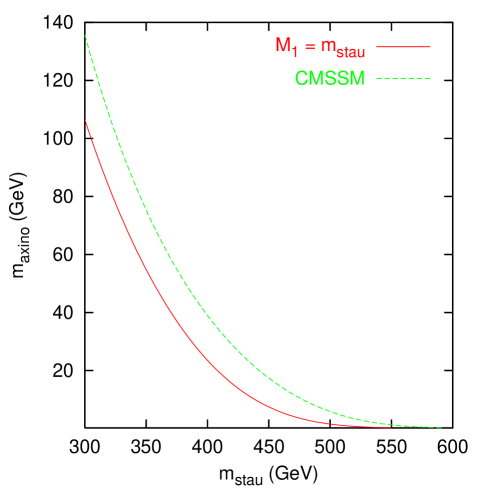
It is important to note that the condition (25) on the axino mass does not guarantee that axinos are produced in sufficient numbers to constitute the dark matter, but merely that, if they are then the decays of parent staus would not disrupt nucleosynthesis. Later we will identify regions of the parameter space where NTP is dominant and the axino density is in the preferred CDM range.

4 Relic Abundance of Axinos

In computing the relic number density $n_{\tilde{a}}$ of axinos we will follow the procedure described in detail in [13, 16]. Here we merely briefly summarize its main points.

As regards TP, the number density of axinos $n_{\tilde{a}}$ can be obtained by integrating the Boltzmann equation with both scatterings and decays of particles in the plasma included. Since $n_{\tilde{a}}$ is well below the equilibrium one for $T_{\rm R}\ll f_{a}$, we can neglect inverse processes. In terms of yield

$$Y^{\rm TP}_{\tilde{a}}=\frac{n_{\tilde{a}}^{\rm TP}}{s}=\sum_{i}Y^{\rm dec}_{i}+\sum_{i,j}Y^{\rm scat}_{i,j},$$ (26)

where $s=(2\pi^{2}/45)g_{s\ast}T^{3}$ is the entropy density, and normally $g_{s\ast}=g_{\ast}$ in the early Universe. By changing variables from the cosmic time $t$ to the temperature $T$, we can write the two solutions of the Boltzmann differential equation easily in integral form

$$Y^{\rm dec}_{i}(T_{0}) = \int_{T_{0}}^{T_{\rm R}}dT\,\frac{\langle\Gamma(i\rightarrow\,\tilde{a}+\cdots)\rangle n_{i}}{sHT}$$ (27)

$$Y^{\rm scat}_{i,j}(T_{0}) = \int_{T_{0}}^{T_{\rm R}}dT\,\frac{\langle\sigma(i+j\rightarrow\,\tilde{a}+\cdots)\rangle n_{i}n_{j}}{sHT}.$$ (28)

where we have considered the evolution from the reheating temperature after inflation, $T_{\rm R}$, down to the present temperature $T_{0}$.

In computing $Y^{\rm dec}_{i}$, in addition to the previously considered decays of gluinos [13] and (s)quarks [16], we now include for consistency the decays of the staus that are generated by the couplings (11) and (12), even though their effect is usually negligible. Also scatterings arising from these effective couplings invariably give subdominant contributions [13, 16] and will be neglected here. The relic abundance due to thermal production is then calculated by using the formula

$$m_{\tilde{a}}Y_{\tilde{a}}\simeq 0.36\,\mbox{eV}\left(\Omega_{\tilde{a}}^{\rm TP}h^{2}\over 0.1\right).$$ (29)

In order to evaluate the axino relic abundance generated through NTP processes we first compute the relic number density of NLSPs after they freeze out from the plasma. In the case of the neutralino, we include all tree–level two–body neutralino processes of pair–annihilation and co–annihilation with the charginos, next–to–lightest neutralinos and sleptons. This is a standard method which allows us to accurate compute $\Omega_{\chi}h^{2}$ in the usual case when the lightest neutralino is the LSP. We further extend the above procedure to the case when it is the lightest stau ${\tilde{\tau}}_{1}$ that is the NLSP. We include all stau–stau annihilation and stau–neutralino co-annihilation processes. In both cases we solve the Boltzmann equation numerically and properly take into account resonance and new final–state threshold effects. The procedure has been described in detail in [35].

Since all the NLSPs subsequently decay into axinos, a simple relation holds

$$\Omega^{\rm NTP}_{\tilde{a}}=\frac{m_{\tilde{a}}}{m_{\rm NLSP}}\Omega_{\rm NLSP}.$$ (30)

In the following, we will first illustrate the impact of the cosmological constraints on the plane ($m_{1/2},m_{0}$) in the CMSSM without the axino, in which case the LSP is normally the lightest neutralino or the stau.

5 DM in the CMSSM without the Axino LSP

In contrast to the general MSSM, mass spectra of the CMSSM are tightly inter–related. This is because the model is defined in terms of only the usual five free parameters: $\tan\beta$, the common gaugino mass $m_{1/2}$, the common scalar mass $m_{0}$, the common trilinear soft scalar coupling $A_{0}$ and ${\rm sgn}(\mu)$ – the sign of the supersymmetric Higgs/higgsino mass parameter $\mu$. For a fixed value of $\tan\beta$, physical masses and couplings are obtained by running various mass parameters, along with the gauge and Yukawa couplings, from their common values at $M_{\rm GUT}$ down to $m_{Z}$ by using the renormalization group (RG) equations. The large top quark Yukawa coupling tends to push $m_{H_{2}}^{2}$ to negative values around the electroweak scale. Therefore electroweak symmetry is spontaneously broken and $\mu^{2}$ is determined, but not its sign.

Experimental and cosmological constraints on the CMSSM are usually presented in the ($m_{1/2},m_{0}$) plane for various representative choices of $\tan\beta$ and other relevant parameters. In this paper, we will not attempt a detailed study of the CMSSM. Instead, we will aim at demonstrating that very different patterns arise by assuming the standard scenario and that with the axino LSP.

Figure 5: The (${m_{1/2}},{m_{0}}$) plane for the standard scenario without the axino LSP, and for ${\tan\beta=10,A_{0}=0}$ and $\mu>0$. In the leftmost (red) region marked “excluded by LEP” the chargino (to the left of a solid line) or the light Higgs is too light. In the tiny dark green band marked “$\Omega_{\chi}h^{2}\;(2\,\sigma)$” $0.095<\Omega_{\chi}h^{2}<0.130$, while in the orange region labeled “$\Omega_{\chi}h^{2}$ too large” $\Omega_{\chi}h^{2}$ exceeds the upper limit. In the white region $\Omega_{\chi}h^{2}$ is less than the favored $2\,\sigma$ range but otherwise allowed.

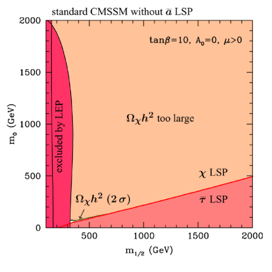
In Fig. 5, we show the plane ($m_{1/2},m_{0}$) for $\tan\beta=10$, $A_{0}=0$ and for $\mu>0$. In the absence of the axino, the lightest neutralino is the LSP above a solid red line, while in the wedge below it the LSP is the lighter stau ${\tilde{\tau}}_{1}$. The red region on the left is excluded by LEP lower bounds on the mass of the chargino $m_{\chi_{1}^{\pm}}>104\,\mbox{GeV}$ (far-most solid line) and the light Higgs $m_{h}\mathrel{\hbox to0.0pt{\lower 4.0pt\hbox{\hskip 1.0pt$\sim$}\hss}\raise 1.0pt\hbox{$>$}}114.4\,\mbox{GeV}$ [36]. In the CMSSM without the axino LSP, the wedge is considered to be excluded as it would give an electrically charged stable relic. Likewise, most of the region of neutralino LSP is excluded due to the relic abundance $\Omega_{\chi}h^{2}$ exceeding current bounds. For a stable relic we will require that its relic abundance falls into the $2\,\sigma$ range

$$0.095<\Omega_{{\rm CDM}}h^{2}<0.130$$ (31)

which follows from combining WMAP results [33] with other recent measurements of the CMB. In Fig. 5, the constraint (31) is fulfilled only in a very narrow (green) band just above and along the red line. In this case, neutralino pair annihilation is inefficient because the sleptons and squarks are already too heavy to reduce $\Omega_{\chi}h^{2}$ through $t$–channel processes. Nor are the heavy Higgs scalars $H$ and $A$ light enough to allow for resonant enhancements, although this becomes the case at very large $\tan\beta\mathrel{\hbox to0.0pt{\lower 4.0pt\hbox{\hskip 1.0pt$\sim$}\hss}\raise 1.0pt\hbox{$>$}}50$ which we do not consider here. The mechanism that comes to the rescue is the neutralino co–annihilation with ${\tilde{\tau}}_{1}$ [6], which however, for $\tan\beta=10$ considered here, is efficient only for $m_{1/2}\mathrel{\hbox to0.0pt{\lower 4.0pt\hbox{\hskip 1.0pt$\sim$}\hss}\raise 1.0pt\hbox{$<$}}500\,\mbox{GeV}$. In the narrow white region below the green band, $\Omega_{\chi}h^{2}$ is less than the favored range of (31). Except for these two, the rest of the ($m_{1/2},m_{0}$) plane is cosmologically excluded.

Clearly, the standard paradigm is highly constrained. We will now proceed to compare it with the case of axino as the LSP and CDM. As we will see, the form of the cosmological constraint will in general become not only very different but also will strongly depend on the axino mass and the reheat temperature.

Figure 6: The (${m_{1/2}},{m_{0}}$) plane for axino LSP with $m_{\tilde{a}}=1\,\mbox{GeV}$ and for $f_{a}=10^{11}\,\mbox{GeV}$, ${\tan\beta=10,A_{0}=0}$ and $\mu>0$. In the left panel, $T_{R}=200\,\mbox{GeV}$, in the right, $400\,\mbox{GeV}$. The dark green (orange, white) regions correspond to $0.095<\Omega_{\tilde{a}}h^{2}<0.130$ ($\Omega_{\tilde{a}}h^{2}$ too large and excluded, too small but otherwise allowed).

6 DM in the CMSSM with the Axino LSP

As summarized in the Introduction, if the axino is light, $m_{\tilde{a}}\mathrel{\hbox to0.0pt{\lower 4.0pt\hbox{\hskip 1.0pt$\sim$}\hss}\raise 1.0pt\hbox{$<$}}10\,\mbox{MeV}$ (while still remaining a cold DM candidate, i.e. $m_{\tilde{a}}\mathrel{\hbox to0.0pt{\lower 4.0pt\hbox{\hskip 1.0pt$\sim$}\hss}\raise 1.0pt\hbox{$>$}}100\,\mbox{keV}$), then thermal production is the dominant source of axinos, and non–thermal production can be neglected. The reheat temperatures favored by cosmology (such as to give $\Omega_{\tilde{a}}h^{2}\sim 0.1$) are in the few hundred  TeV range, independently of $m_{1/2}$ and $m_{0}$ for any sensible values of these parameters.

If the axino mass is increased to $1\,\mbox{GeV}$, non–thermal production is typically still negligible. However, the cosmologically favored range $\Omega_{\tilde{a}}h^{2}$ then requires $T_{\rm R}\mathrel{\hbox to0.0pt{\lower 4.0pt\hbox{\hskip 1.0pt$\sim$}\hss}\raise 1.0pt\hbox{$<$}}{\cal O}(1\,\mbox{TeV})$ at which point squark and slepton decays in TP start playing a major role. This can be seen in Figs. 7 and 9 of [16] in the case of squark decays. In particular, one can see in Fig. 9 of [16] that, at fixed $m_{\tilde{a}}$, as squark masses decrease, a maximum $T_{\rm R}$ allowed by $\Omega_{\tilde{a}}h^{2}<0.13$ also decreases. A convenient way to present this is to invert the reasoning and to consider the cosmologically favored ranges of squark and slepton masses at fixed $T_{\rm R}$. Since these increase with $m_{1/2}$ and $m_{0}$, this will be reflected in cosmologically favored regions of the ($m_{1/2},m_{0}$) plane at given fixed values of $m_{\tilde{a}}$ and $T_{\rm R}$.

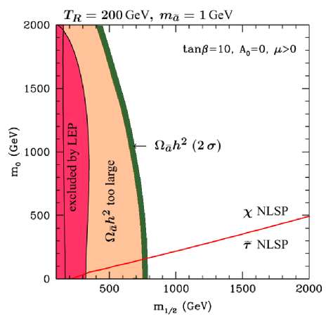
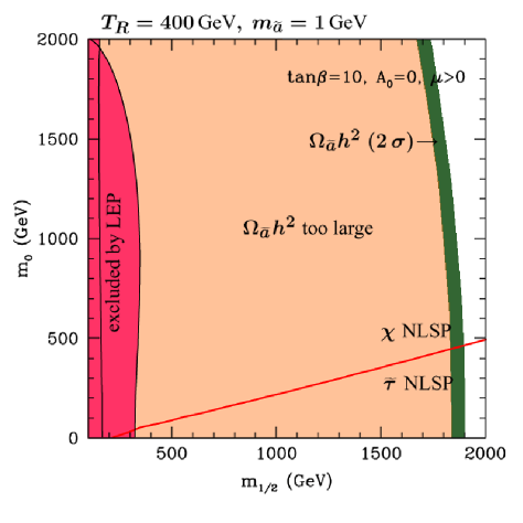
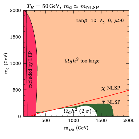
In the left panel of Fig. 6 the ($m_{1/2},m_{0}$) plane is shown for a reheat temperature of $200\,\mbox{GeV}$, while on the right this is increased to $400\,\mbox{GeV}$. In both panels $m_{\tilde{a}}=1\,\mbox{GeV}$. Other relevant parameters have been set to the following values: $f_{a}=10^{11}\,\mbox{GeV}$, $\tan\beta=10$, $A_{0}=0$, and $\mu>0$. The red line divides the neutralino and stau NLSP regions. Below the line, the stau is the NLSP, while above it the neutralino. As in Fig. 5, the red band along the $m_{0}$ axis is excluded by imposing the LEP bounds on the chargino and Higgs mass. The cosmologically favored range is coloured green, while the region excluded by the requirement that axinos should not overclose the Universe ($\Omega_{\tilde{a}}h^{2}\mathrel{\hbox to0.0pt{\lower 4.0pt\hbox{\hskip 1.0pt$\sim$}\hss}\raise 1.0pt\hbox{$<$}}0.130$) is marked in orange. The white regions are cosmologically allowed, but not favored, i.e. $\Omega_{\tilde{a}}h^{2}\mathrel{\hbox to0.0pt{\lower 4.0pt\hbox{\hskip 1.0pt$\sim$}\hss}\raise 1.0pt\hbox{$<$}}0.095$.

In both panels, it is clear that thermally produced axinos exclude a region closer to the $m_{0}$ axis, while there is a cosmologically favored strip further out. As $T_{\rm R}$ is increased, the excluded region grows and the favored region is pushed farther out to the right. This can be understood by again examining Fig. 7 of [16]: at fixed sfermion and gluino masses, as $T_{\rm R}$ is taken to larger values, the corresponding yield and therefore (at fixed $m_{\tilde{a}}$) $\Omega_{\tilde{a}}h^{2}$ increase. The important point to note here is that a portion of the cosmologically favored region lies in the stau NLSP wedge, which is traditionally thought to be excluded. Note that the bounds of Fig. (4) are not applicable here because NTP is negligible in this region and also that other BBN bounds are irrelevant for cold axinos [13], similarly as for neutralino CDM.

We now consider the other limit in which the axino is as heavy as possible, but slightly lighter than the NLSP in order to avoid a strong phase space suppression in the NLSP decay. In this regime non–thermal production is no longer negligible. In fact, at low enough $T_{\rm R}$, as the yield due to TP becomes too small, it is NTP that starts providing enough axinos. Again, we refer the reader to Figs. 7–9 of [16]. We plot the case of $m_{\tilde{a}}\sim m_{\rm NLSP}$, in Fig. 7. In the left panel the reheat temperature is $50\,\mbox{GeV}$, while on the right this is increased to $200\,\mbox{GeV}$. The other parameters are set to the same values as in Fig. 6.

Figure 7: The (${m_{1/2}},{m_{0}}$) plane for an axino only slightly less massive than the NLSP, with $f_{a}=10^{11}\,\mbox{GeV}$, ${\tan\beta=10}$, $A_{0}=0$, and $\mu>0$. In the left panel, $T_{R}=50\,\mbox{GeV}$, in the right, $200\,\mbox{GeV}$. The notation follows that of Fig. 6.

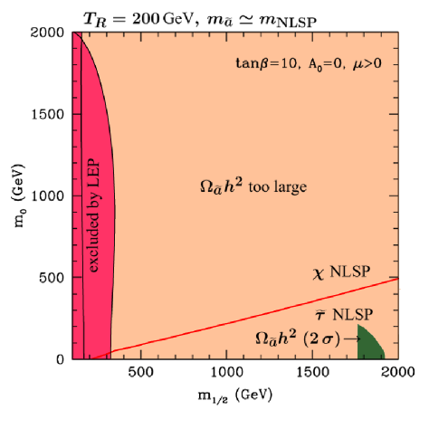
In the left panel, in which $T_{\rm R}=50\,\mbox{GeV}$, the thermal production of axinos now plays a subdominant role. This is reflected in the fact that the green region of favored $\Omega_{\tilde{a}}h^{2}$ in the neutralino NLSP section, at $m_{0}\sim 100\,\mbox{GeV}$, coincides with the green region of the neutralino LSP in Fig. 5 as a result of the relation (30). For the same reason, at $m_{1/2}\simeq 700\,\mbox{GeV}$, the green region starts to extend further down into the stau NLSP wedge, along the line dividing the stau and neutralino NLSP sections, as co–annihilations between the neutralino and the stau keep the LSP density within the expected range. Further to the right, the co–annihilation ceases to be effective but stau decays provide enough $\Omega_{\tilde{a}}h^{2}$ for a limited range of $m_{{\tilde{\tau}}_{1}}$. It is interesting to note that the majority of the cosmologically favored region now lies in the stau NLSP wedge. In this region the lower bound on the axino mass given in Fig. 4 as CMSSM applies and it is in our case satisfied. Note also, that even at such low temperature, the NLSP is completely thermalized in the whole (${m_{1/2}},{m_{0}}$) plane.

In the right panel, in which $T_{\rm R}=200\,\mbox{GeV}$, TP can no longer be neglected, and in fact thermally produced axinos overclose the Universe if the neutralino is the NLSP. However, there is still a green region at $m_{1/2}\simeq 1900\,\mbox{GeV}$ in the stau NLSP region, in which TP and NTP axinos together form the cosmologically favored abundance of CDM.

The left panel of Fig. 6 and the right panel of Fig. 7 allow one to see the effect of increasing $m_{\tilde{a}}$ at fixed $T_{\rm R}$. The cosmologically favored band due to TP axinos moves to the right along the $m_{1/2}$ axis, in a similar way to the effect of increasing $T_{\rm R}$. This amounts to increasing sfermion and gluino masses which in turn will increase the importance of NTP relative to TP, as can be seen in Fig. 7 of [16]. As a result, in the right panel of Fig. 7, NT production gives too much relic density in the cosmologically favored band for TP axinos, except for the small region in the corner of small $m_{0}$ and large $m_{1/2}$. In the left part of this region, TP axinos provide the required abundance, and as you move to the right within the region TP axinos become subdominant and NTP axinos provide the necessary abundance, before eventually producing too many of them.

If one increased the reheat temperature further up one would exclude the region where NTP axinos can be CDM, and pushed the region where TP axinos can perform this function to values of $m_{1/2}$ larger than those plotted here. On the other hand, decreasing the reheat temperature below a few  GeV would have the effect of suppressing the relic abundance of NLSPs, so that neither TP nor NTP could provide axino CDM. We will not investigate this possibility here.

7 Conclusion

The Constrained MSSM provides a popular and predictive framework for analyzing properties of low–energy SUSY. While theoretical assumptions and experimental bounds from LEP and $b\to s\gamma$ provide significant constraints on the parameter space, it is the cosmological relic density of the LSP as cold DM and the requirement of its electric neutrality that rule out most of the ($m_{1/2},m_{0}$) plane and, for $\tan\beta\mathrel{\hbox to0.0pt{\lower 4.0pt\hbox{\hskip 1.0pt$\sim$}\hss}\raise 1.0pt\hbox{$<$}}50$, allow for only a tiny region in the plane.

In this paper, we have considered the cosmological bounds on the scenario in which the LSP is not the usual neutralino but instead the axino. Our purpose was not to provide an exhaustive scan of the CMSSM but to illustrate with a few examples the very different patterns that arise. We concentrated on two cases of a fairly light axino $m_{\tilde{a}}=1\,\mbox{GeV}$ and of $m_{\tilde{a}}\sim m_{\rm NLSP}$ where the NLSP was either the neutralino or the lighter stau. In computing the axino relic abundance we included both thermal and non–thermal production processes. Our results are a function of $T_{\rm R}$ which in all cases had to be rather low, below a few hundred  GeV in order to give the right amount of axino CDM. We further included constraints from nucleosynthesis which are important for lighter axinos and staus.

The cosmologically favored regions consistent with axino CDM relic abundance are in general very different from the usual scenario. Depending on $m_{\tilde{a}}$ and/or $T_{\rm R}$, basically nearly any point in the ($m_{1/2},m_{0}$) plane can become cosmologically allowed. This is true for both the regions where the NLSP is the neutralino or the lighter stau. This significantly relaxes the cosmological bounds obtained in the absence of the axino.

From the point of view of collider phenomenology, with the lifetime of ${\cal O}(1\sec)$, the NLSP would appear stable in a detector. However, if the NLSP is the neutralino, then very likely one would find its relic abundance (calculated under the assumption that it is the true LSP) to significantly exceed $0.13$. The NLSP could also be electrically charged (stau), or even colored (stop) – the possibility we have not investigated here. In conclusion, in collider studies of the CMSSM parameter space, both the apparently cosmologically excluded bulk of the $(m_{1/2},m_{0})$ plane where the neutralino is the NLSP and the wedge at its bottom where the lighter stau is the NLSP, should be given equal attention as the narrow regions preferred by the standard paradigm.