Radiative Corrections to the Azimuthal Asymmetry
in Transversely Polarized Møller Scattering

Abstract

Experiment E158 at SLAC can measure an azimuthal asymmetry in single-spin, transversely polarized Møller scattering, $e^{-\uparrow}e^{-}\rightarrow e^{-}e^{-}$, which arises from a QED rescattering phase. We recompute the leading-order (one-loop) asymmetry, confirming previous results, and calculate the leading logarithmic QED corrections due to initial-state radiation from the beam and target electrons, and due to final-state radiation. The size of these radiative corrections is quite sensitive to experimental details, such as the acceptance in energy and in polar angle of the scattered electron. For E158, the corrections are modest, increasing the parts-per-million asymmetry by roughly 1%.

I Introduction

Single-spin triple product asymmetries, or asymmetries arising from transverse polarization, play a special role in scattering theory because they are directly sensitive to rescattering phases. An operator of the form $O\equiv{\bf S}\cdot({\bf k}\times{\bf k}^{\prime})$, where ${\bf S}$ is a spin and ${\bf k}$ and ${\bf k}^{\prime}$ are two different particle momenta, is odd under a “naive” time-reversal operation which reverses all spins and momenta, but does not exchange initial and final states. A nonzero value for $O$ stems from terms in the covariant scattering amplitude that are proportional to the Levi-Civita tensor $\epsilon_{\mu\nu\rho\sigma}$, which always appears accompanied by a factor of $i$. Hence, in the absence of CP violation, a nonzero expectation value $\langle O\rangle$ requires an absorptive (imaginary) part for the amplitude, ${\rm Im}\,T\neq 0$, which can be generated by rescattering, for example by one-loop diagrams containing intermediate two-particle cuts.

There have been many theoretical and experimental studies of single-spin transversely-polarized asymmetries in a variety of contexts. For instance, in the decay of a polarized neutron, $n^{\uparrow}\rightarrow p+e^{-}+\bar{\nu}_{e}$, an expectation value for ${\bf S}_{n}\cdot({\bf k}_{e}\times{\bf k}_{\nu})$ is produced by QED final-state interactions, which can therefore mask truly ${\rm T}$-odd effects JTW . Analogous single-spin observables in the decay of a polarized $Z$ boson to three hadronic jets, stemming from QCD and electroweak final-state interactions, have been studied theoretically eezqqg and bounded experimentally SLDeezqqg . QCD final-state interactions can also play a role in generating azimuthal single-spin asymmetries in semi-inclusive pion leptoproduction off polarized protons at leading twist BHS . Similarly, a phase in the time-like electromagnetic proton form-factor from QCD final-state interactions can be detected by measuring transverse proton polarization in the reaction $e^{+}e^{-}\rightarrow p\bar{p}$ pformfactor .

As a final example, QED rescattering phases produce an azimuthal asymmetry in the elastic scattering of electrons off transversely polarized protons, $ep^{\uparrow}\rightarrow ep$, or transverse final-state polarization in the time-reversed reaction $ep\rightarrow ep^{\uparrow}$. The QED asymmetry receives contributions not only from two-photon exchange with a single proton in the intermediate state, but also from inelastic hadronic intermediate states; the latter terms are difficult to compute directly, although they can be bounded experimentally eptransverse .

Perhaps the cleanest setting for studying such asymmetries is in a process dominated by QED, such as transversely polarized Møller scattering, $e^{-\uparrow}e^{-}\rightarrow e^{-}e^{-}$. Experiment E158 at SLAC performs Møller scattering of $\approx 45$ GeV polarized electrons off unpolarized target electrons at rest. The prime goal of E158 is to measure the parity-violating right-left asymmetry in the cross section for longitudinal beam polarization, $A_{PV}=(\sigma_{R}-\sigma_{L})/(\sigma_{R}+\sigma_{L})$. The right-left asymmetry is sensitive to $Z$ boson exchange, and potentially to new physics, such as a new $Z$ boson or contact interactions. The first measurement has yielded $A_{PV}=(-175\pm 30({\rm stat.})\pm 20({\rm syst.}))\times 10^{-9}$ E158PV . While most of the E158 data were taken with the electron beam polarized longitudinally in order to accomplish this measurement, a fraction of the running was carried out with transverse electron polarization, enabling the measurement of an azimuthal asymmetry,

$$A_{T}(\phi)\equiv{2\pi\over\sigma^{\uparrow}+\sigma^{\downarrow}}{d(\sigma^{\uparrow}-\sigma^{\downarrow})\over d\phi}\propto{\bf S}_{e}\cdot({\bf k}_{e}\times{\bf k}^{\prime}_{e})\propto\sin\phi,$$ (1)

where ${\bf S}_{e}$ is the spin of the incoming electron, with momentum ${\bf k}_{e}$, and $\phi$ is the azimuthal angle of the scattered electron (with momentum ${\bf k}^{\prime}_{e}$) around the beam direction, measured from the direction of the transverse polarization.

In contrast to $A_{PV}$, a nonzero azimuthal asymmetry $A_{T}(\phi)$ can be generated by QED interactions alone. The calculation of $A_{T}(\phi)$ for transversely polarized Møller scattering at the leading one-loop order was performed by Barut and Fronsdal in 1960 BarutFronsdal , and by DeRaad and Ng in 1974 DeRaadNg . Because only the absorptive part of the scattering amplitude contributes to this observable, an $s$-channel cut is required. Hence only the box Feynman diagram enters, plus the version obtained by exchanging the two identical outgoing electron legs, as depicted in fig. 1. Besides the rescattering phase, the effect requires an electron helicity flip. For center-of-mass (CM) energies much larger than the electron mass, $\sqrt{s}\gg m_{e}$, therefore, it takes the form $A_{T}(\phi)=\alpha{m_{e}\over\sqrt{s}}f(\theta)\sin\phi$, where $\alpha$ is the fine structure constant, $\phi$ and $\theta$ are respectively the azimuthal and (CM frame) polar scattering angles, and $f$ is a function of $\theta$.

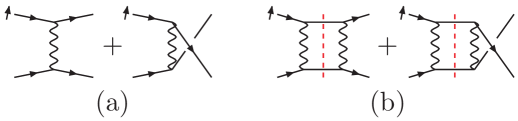
Figure 1: (a) Tree-level graphs for electron-electron scattering. (b) One-loop graphs contributing to the azimuthal asymmetry for transverse polarization. Because an absorptive part in the $s$ channel is required (the cut is indicated by the dashed line), only box diagrams contribute. The transverse spin of the beam electron is indicated by the arrow next to that incoming line.

Since there are two identical electrons in the final state, $f(\theta)$ must be odd under $\theta\rightarrow\pi-\theta$; that is, a symmetric acceptance in $\theta$ (in an unsegmented detector) will wash out the asymmetry in $\phi$. The E158 detector is well segmented in $\phi$ (twelve-fold), but coarsely segmented in $\theta$ (only two-fold). Fortuitously, the $\theta$ acceptance is almost entirely in the backward hemisphere in the CM frame, leaving the sensitivity of E158 to $A_{T}(\phi)$ quite high.

The E158 CM energy is roughly 200 MeV, so the asymmetry is of order $\alpha m_{e}/\sqrt{s}\sim 10^{-5}$. This may seem small, but it is two orders of magnitude larger than the electroweak asymmetry $A_{PV}$. Even though only a relatively small fraction of the data was taken with transversely polarized electrons, a precision of the order of a few percent can be achieved for $A_{T}(\phi)$. One can either test QED at this level, or reverse the logic and use the QED prediction as a detector calibration or polarimeter Woods .

At the percent level of precision, it becomes important to investigate the next-to-leading order (NLO), or ${\cal O}(\alpha^{2})$, QED radiative corrections to $A_{T}(\phi)$. The full ${\cal O}(\alpha^{2})$ calculation of the asymmetry requires two-loop scattering amplitudes for $e^{-\uparrow}e^{-}\rightarrow e^{-}e^{-}$ and one-loop scattering amplitudes for $e^{-\uparrow}e^{-}\rightarrow e^{-}e^{-}\gamma$. For $\sqrt{s}\gg m_{e}$, as in E158 kinematics, it would suffice to compute these amplitudes in the limit where one takes $m_{e}\rightarrow 0$ after extracting the leading $m_{e}/\sqrt{s}$ behavior from the diagrams. This computation should be feasible, because it is known how to perform all the relevant two-loop four-point integrals DoubleBoxes and one-loop five-point integrals BDKPentagon in this limit in dimensional regularization. (Similar amplitudes without transverse polarization have already been computed SimilarAmps .)

In the present paper, we calculate the largest of the ${\cal O}(\alpha^{2})$ corrections, those that are enhanced by the large logarithm $\ln(s/m_{e}^{2})$ due to collinear singularities in initial state radiation from both the incoming beam electron and the target electron, as well as final-state radiation. The amplitude for $e^{-\uparrow}e^{-}\rightarrow e^{-}e^{-}\gamma$ factorizes in these collinear limits, so that its full kinematic dependence is not required. In an electron structure function approach ElectronSF , analogues of the DGLAP splitting kernels DGLAP enter our computation. In the case of target radiation and final-state radiation, only the unpolarized kernels are required. However, the radiation from the transversely polarized beam electron also involves the analogues of kernels for the evolution of transversely polarized quark distributions AM . These kernels can be obtained from the standard longitudinally polarized splitting amplitudes by a change of basis.

We find that the magnitude of the leading-log NLO corrections is quite sensitive to the experimental cuts. Initial state radiation (ISR), for example, lowers the effective value of $s$, which could enhance the asymmetry, since the leading-order asymmetry is proportional to $m_{e}/\sqrt{s}$. More importantly, ISR also skews the relation between polar angles in the post-radiation $e^{-}e^{-}$ CM frame and the lab frame, changing the effective CM polar angle acceptance of the experiment. Final state radiation (FSR) does not have either of these properties, and typically produces smaller corrections to the asymmetry.

This paper is organized as follows. In section II we establish our notation and review the leading-order azimuthal asymmetry prediction BarutFronsdal ; DeRaadNg . In section III we describe the leading-log NLO corrections and present numerical results for an experimental arrangement similar to E158. In section IV we present our conclusions. In appendix A we give a derivation of the kernel needed for evolution of the transversely polarized electron distribution.

II Notation and Leading-Order Results

We consider the process

$$e^{-\uparrow}(k_{1})\ +\ e^{-}(k_{2})\ \ \rightarrow\ \ e^{-}(k_{1}^{\prime})\ +\ e^{-}(k_{2}^{\prime})\ \ [\ +\ \gamma(k_{\gamma})\ ],$$ (2)

where the photon is only present at next-to-leading order. We use a right-handed $xyz$ coordinate system, writing momenta $k^{\mu}=(k_{t},k_{x},k_{y},k_{z})$. We take the energy of the beam electron in the lab frame to be $E$, and its momentum to be in the $z$ direction: $k_{1}=(E,0,0,\sqrt{E^{2}-m_{e}^{2}})$. We let its polarization be in the negative $x$ direction . In the lab frame, the unpolarized target electron is at rest, $k_{2}=(m_{e},0,0,0)$. The momentum of the detected scattered electron is $k_{1}^{\prime}=(E_{\mbox{\tiny lab}},\sqrt{E_{\mbox{\tiny lab}}^{2}-m_{e}^{2}}\sin\theta_{\mbox{\tiny lab}}\cos\phi,\sqrt{E_{\mbox{\tiny lab}}^{2}-m_{e}^{2}}\sin\theta_{\mbox{\tiny lab}}\sin\phi,\sqrt{E_{\mbox{\tiny lab}}^{2}-m_{e}^{2}}\cos\theta_{\mbox{\tiny lab}})$; its azimuthal angle $\phi$ increases from $0$ in the positive $x$ direction, through $\pi/2$ in the positive $y$ direction.

The Born-level differential cross section for Møller scattering, from the tree diagrams in fig. 1a, is

$$\frac{d\sigma^{\mbox{\tiny Born}}}{d\Omega}\bigg{|}_{\rm exact}=\frac{\alpha^{2}}{2s}\cdot\frac{(t^{2}+tu+u^{2})^{2}+4m_{e}^{2}(m_{e}^{2}-t-u)(t^{2}-tu+u^{2})}{t^{2}u^{2}}\,,$$ (3)

where $s=(k_{1}+k_{2})^{2}=2m_{e}(E+m_{e})$, $u=(k_{1}^{\prime}-k_{2})^{2}=-2m_{e}(E_{\mbox{\tiny lab}}-m_{e})$, $t=(k_{1}^{\prime}-k_{1})^{2}=4m_{e}^{2}-s-u$. (We include the statistical factor of 1/2 for identical electrons in $d\sigma/d\Omega$, so such expressions should be integrated over two-body phase-space for non-identical particles.)

The leading term in the cross section containing azimuthal dependence arises at order $\alpha^{3}$, from the interference between the tree diagrams in fig. 1a and the box diagrams in fig. 1b. The $\phi$-dependence at this order is given by BarutFronsdal ; DeRaadNg

$$\frac{d\sigma^{\phi}}{d\Omega}\bigg{|}_{\rm exact} = -{\alpha^{3}\over 8}{m_{e}\over\sqrt{s}}\sin\theta\sin\phi\sqrt{1-{4m_{e}^{2}\over s}}{1\over t^{2}u^{2}}$$ (4)

$$\hskip 5.69046pt\times\biggl{[}3(s-4m_{e}^{2})\biggl{(}t(u-s+2m_{e}^{2})\ln\Bigl{(}{-t\over s-4m_{e}^{2}}\Bigr{)}-u(t-s+2m_{e}^{2})\ln\Bigl{(}{-u\over s-4m_{e}^{2}}\Bigr{)}\biggr{)}-2(t-u)tu\biggr{]}\,.$$

We have reproduced this result independently.

Equations (3) and (4) include the exact dependence on the electron mass. However, in computing the NLO leading logarithms in $s/m_{e}^{2}$, we shall drop the terms suppressed by powers of $m_{e}^{2}/s$ in the leading-order asymmetry. The error induced by omitting these terms, for E158 kinematics, is much smaller than the size of the ${\cal O}(\alpha^{2}\ln(s/m_{e}^{2}))$ corrections. The Born-level and leading $\phi$-dependent cross sections then become,

$$\frac{d\sigma^{\mbox{\tiny Born}}}{d\Omega}=\frac{\alpha^{2}}{2s}\cdot\biggl{(}{t^{2}+tu+u^{2}\over tu}\biggr{)}^{2}\,,$$ (5)

$$\frac{d\sigma^{\phi}}{d\Omega}=-{\alpha^{3}\over 8}{m_{e}\over\sqrt{s}}\sin\theta\sin\phi\ {1\over t^{2}u^{2}}\biggl{[}3s\biggl{(}t(u-s)\ln\Bigl{(}{-t\over s}\Bigr{)}-u(t-s)\ln\Bigl{(}{-u\over s}\Bigr{)}\biggr{)}-2(t-u)tu\biggr{]}\,,$$ (6)

and the kinematics can be simplified to

$$s=2m_{e}E,\qquad t=-2EE_{\mbox{\tiny lab}}(1-\cos\theta_{\mbox{\tiny lab}})=-{s\over 2}(1-\cos\theta),\qquad u=-2m_{e}E_{\mbox{\tiny lab}}=-{s\over 2}(1+\cos\theta),$$ (7)

$$E_{\mbox{\tiny lab}}={E\over 2}(1+\cos\theta),\qquad\cos\theta_{\mbox{\tiny lab}}=1-{m_{e}\over E}{1-\cos\theta\over 1+\cos\theta},$$ (8)

with $\theta$ the CM frame polar scattering angle.

Writing the asymmetry as

$$A_{T}(\phi)\equiv{2\pi\over\sigma^{\uparrow}+\sigma^{\downarrow}}{d(\sigma^{\uparrow}-\sigma^{\downarrow})\over d\phi}\equiv\alpha_{T}\cdot\sin\phi\,,$$ (9)

we have

$$\alpha_{T}^{LO}={1\over\sin\phi}{d\sigma^{\phi}/d\Omega\over d\sigma^{\mbox{\tiny Born}}/d\Omega}\,.$$ (10)

In fig. 2 the leading-order asymmetry coefficient, $\alpha_{T}^{LO}$, is plotted as a function of CM polar angle, $\cos\theta$, for a beam energy of $E=46$ GeV, or $\sqrt{s}\approx 217$ MeV. We set $\alpha=\alpha(\sqrt{s})=1/135.9$ here. (E158 probes central scattering in the CM frame, with $|t|$ and $|u|$ ranging between $0.3s$ and $s$, so the difference between $\alpha(\sqrt{s})$ and $\alpha(\sqrt{|t|})$ or $\alpha(\sqrt{|u|})$ is negligible, less than 0.1%.) The asymmetry is of order parts per million at this energy.

Figure 2: The azimuthal asymmetry coefficient at leading order, $\alpha_{T}^{LO}$, as a function of $\cos\theta$, for $E=46$ GeV, $\sqrt{s}\approx 217$ MeV. The vertical dotted lines indicate the approximate acceptance of E158 for leading-order kinematics.

Note that $\alpha_{T}^{LO}$ is odd under $\theta\leftrightarrow\pi-\theta$, or equivalently, that eq. (6) is odd under $t\leftrightarrow u$. This asymmetry is a consequence of having two identical electrons in the final state. In the CM frame, if one electron is at an angle $(\theta,\phi)$, the other (at leading order) is at $(\pi-\theta,\phi+\pi)$. Because $\sin\phi$ is odd under $\phi\leftrightarrow\phi+\pi$, the coefficient $\alpha_{T}^{LO}$ must be odd under $\theta\leftrightarrow\pi-\theta$. The odd behavior means that the integrated asymmetry seen by an experiment integrating over a range in $\cos\theta$ is quite sensitive to the precise acceptance. For example, a symmetric forward-backward acceptance in the CM frame leads to zero asymmetry at leading order. The E158 polar-angle acceptance E158PV , $4.4~{}{\rm mrad}<\theta_{\mbox{\tiny lab}}<7.5~{}{\rm mrad}$, corresponds mainly to the backward CM hemisphere for leading-order kinematics, $-0.4\buildrel<\over{{}_{\sim}}\cos\theta\buildrel<\over{{}_{\sim}}0.1$, as indicated by the dotted lines in fig. 2.

As mentioned in the introduction, the sensitivity to the acceptance could lead to relatively large QED corrections from hard photon radiation, which skews the kinematics of the $e^{-}e^{-}\rightarrow e^{-}e^{-}$ subprocess. In the next section we investigate these corrections in more detail.

III NLO Calculation and Results

The leading-logarithmic QED corrections to the azimuthal asymmetry arise from collinearly enhanced hard photon radiation. These contributions can be divided into beam ($b$), target ($t$), and final-state ($f$) radiation, according to the electron line with which the photon is collinear, as shown in fig. 3. In each of these limits, the $e^{-}e^{-}\rightarrow e^{-}e^{-}\gamma$ cross section factorizes into a collinear splitting probability ElectronSF ; DGLAP , multiplied by the lower-order $e^{-}e^{-}\rightarrow e^{-}e^{-}$ cross section evaluated for boosted kinematics. In the construction of the asymmetry, for the $\phi$-dependent numerator the boosted cross section is provided by $d\sigma^{\phi}/d\Omega$ in eq. (6); for the denominator of the asymmetry it is $d\sigma^{\mbox{\tiny Born}}/d\Omega$ in eq. (5). We still have to pay a factor of $m_{e}/\sqrt{s}$ in $d\sigma^{\phi}/d\Omega$; hence we can neglect powers of $m_{e}/\sqrt{s}$ in the splitting probabilities.

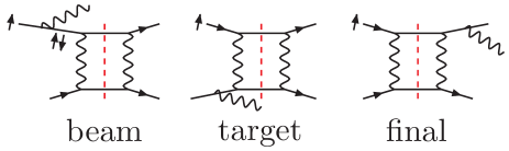
Figure 3: Diagrams contributing to the NLO leading-log-enhanced corrections to the azimuthal asymmetry. These graphs are to be interfered with corresponding graphs for the Born process. The exchange graphs are omitted. Also shown, with short arrows, are the transverse spin states of the initial electron, and of the quasi-on-shell electron line in the case of beam radiation.

Although from the perspective of the lab frame one might not expect radiation off of the target to be important, in the center of mass frame such radiation is on an almost equal footing with radiation from the beam. One difference, though, is that we have to track the transverse polarization of the quasi-on-shell electron in the case of beam radiation, as indicated by the opposing transverse arrows in fig. 3. A dilution of the transverse polarization will accompany the photon radiation in this case.

We let $x$ denote the longitudinal momentum fraction retained by an incoming or outgoing electron, after it has radiated a collinear photon. The $x\rightarrow 1$ limit represents emission of a soft photon. In the leading-log approximation, we neglect the transverse momentum of the photon in computing the boosted kinematics of the $e^{-}e^{-}\rightarrow e^{-}e^{-}$ subprocess. The integral over this small transverse momentum produces an overall factor of $\ln(s/m_{e}^{2})$. The unpolarized splitting probability for massless electrons is well known ElectronSF

$$P(x)={1\over(1-x)_{+}}-{1\over 2}(1+x)+{3\over 4}\delta(1-x),$$ (11)

with the standard “plus” prescription definition,

$$\int_{0}^{1}dx\frac{f(x)}{(1-x)_{+}}\equiv\int_{0}^{1}dx\frac{f(x)-f(1)}{1-x}.$$ (12)

For the case of radiation from the transversely polarized beam, we need to know the probability of a transverse spin flip. This probability is unsuppressed in the massless electron limit, because a transverse polarization state is a coherent superposition of two different longitudinal (helicity) states. Thus a helicity flip is not required, only a different amplitude for the two different electron helicity configurations, for a given photon helicity. In appendix A we perform this computation. The result can also be extracted from the QCD evolution equations for transversely polarized quarks AM , by converting color factors and coupling constants to the QED case:

$$P^{\uparrow\uparrow}(x) = {1\over(1-x)_{+}}-{1\over 4}(3+x)+{3\over 4}\delta(1-x),$$ (13)

$$P^{\uparrow\downarrow}(x) = {1\over 4}(1-x),$$ (14)

where $P^{\uparrow\uparrow}$ ($P^{\uparrow\downarrow}$) is the splitting probability without (with) a transverse spin flip. These probabilities satisfy $P^{\uparrow\uparrow}(x)+P^{\uparrow\downarrow}(x)=P(x)$. It turns out that the $\delta(1-x)$ terms make a vanishing contribution to the azimuthal asymmetry, since they do not disrupt the leading-order kinematics, and the spin-flip probability vanishes in the soft limit $x\rightarrow 1$.

In the case of ISR, because the radiated photon carries momentum, the effective CM energy-squared for the Møller scattering decreases from $s=2m_{e}E$ to $s^{\prime}=xs$. In the case of FSR, the radiation happens after the scattering, so $s^{\prime}=s$. In radiative events, we use $\theta$ to denote the polar angle in the CM frame of the $e^{-}e^{-}\rightarrow e^{-}e^{-}$ subprocess. To take into account experimental cuts, we need to relate $\theta$ and $x$ to the lab variables $\theta_{\mbox{\tiny lab}}$ and $E_{\mbox{\tiny lab}}$. The relations are:

$$s^{\prime} = xs,\qquad E_{\mbox{\tiny lab}}=x{E\over 2}(1+\cos\theta),\qquad\cos\theta_{\mbox{\tiny lab}}=1-{m_{e}\over x\,E}{1-\cos\theta\over 1+\cos\theta}\,,\qquad\hbox{[beam]}$$ (15)

$$s^{\prime} = xs,\qquad E_{\mbox{\tiny lab}}={E\over 2}(1+\cos\theta),\qquad\cos\theta_{\mbox{\tiny lab}}=1-{x\,m_{e}\over E}{1-\cos\theta\over 1+\cos\theta}\,,\qquad\hbox{[target]}$$ (16)

$$s^{\prime} = s,\qquad E_{\mbox{\tiny lab}}=x{E\over 2}(1+\cos\theta),\qquad\cos\theta_{\mbox{\tiny lab}}=1-{m_{e}\over E}{1-\cos\theta\over 1+\cos\theta}\,.\qquad\hbox{[final]}$$ (17)

We define a model experimental acceptance in the lab frame by

$$A:\quad E_{\mbox{\tiny lab}}>E_{\mbox{\tiny min}},\qquad\theta_{\mbox{\tiny min}}<\theta_{\mbox{\tiny lab}}<\theta_{\mbox{\tiny max}}.$$ (18)

Using eqs. (15), (16) and (17) the acceptance $A$ can be translated into acceptances $A_{b}$, $A_{t}$, and $A_{f}$ bounding the integration region for $x$ and $\theta$ in the respective correction terms (and also the region $A_{0}$ which bounds the $\theta$ integral for leading-order, non-radiative events).

Including collinear radiation, the relevant terms in the differential cross section are modified as follows,

$${d\sigma^{\mbox{\tiny Born}}(s)\over d\Omega} \rightarrow {d\sigma^{\mbox{\tiny Born}}(s)\over d\Omega}+{\alpha\over\pi}\ln\Bigl{(}{s\over m_{e}^{2}}\Bigr{)}\sum_{i=b,t,f}\int_{0}^{1}dx\,P_{i}^{\mbox{\tiny Born}}(x){d\sigma^{\mbox{\tiny Born}}(s)\over d\Omega}\,,$$ (19)

$${d\sigma^{\phi}(s)\over d\Omega} \rightarrow {d\sigma^{\phi}(s)\over d\Omega}+{\alpha\over\pi}\ln\Bigl{(}{s\over m_{e}^{2}}\Bigr{)}\sum_{i=b,t,f}\int_{0}^{1}dx\,P_{i}^{\phi}(x){d\sigma^{\phi}(s)\over d\Omega}\,,$$ (20)

where $P_{b}^{\phi}=P^{\uparrow\uparrow}(x)-P^{\uparrow\downarrow}(x)$, $P_{b}^{\mbox{\tiny Born}}=P_{t}^{\mbox{\tiny Born}}=P_{f}^{\mbox{\tiny Born}}=P_{t}^{\phi}=P_{f}^{\phi}=P(x)$. We insert eqs. (19) and (20) into eq. (10), perform the integrals over the respective acceptances in both the numerator and denominator of the asymmetry, expand the result in $\alpha$, and thus obtain for the leading-log-corrected asymmetry coefficient,

$$\alpha_{T}^{LL}=\alpha_{T}^{LO}(1+\delta_{b}+\delta_{t}+\delta_{f}),$$ (21)

where

$$\alpha_{T}^{LO} = {N_{0}\over D_{0}}\,,$$ (22)

$$\delta_{i} = {\alpha(\sqrt{s})\over\pi}\ln\Bigl{(}{s\over m_{e}^{2}}\Bigr{)}\biggl{[}{N_{i}\over N_{0}}-{D_{i}\over D_{0}}\biggr{]}\,,\qquad i=b,t,f.$$ (23)

Here the leading-order integrated results are

$$N_{0}=\int_{A_{0}}d\cos\theta\,{d\sigma^{\phi}(s)\over d\Omega},\qquad D_{0}=\int_{A_{0}}d\cos\theta\,{d\sigma^{\mbox{\tiny Born}}(s)\over d\Omega}\,.$$ (24)

The radiative terms are

$$N_{b} = \int_{A_{b}}dx\,d\cos\theta\,[P^{\uparrow\uparrow}(x)-P^{\uparrow\downarrow}(x)]\,{d\sigma^{\phi}(xs)\over d\Omega},\qquad D_{b}=\int_{A_{b}}dx\,d\cos\theta\,P(x)\,{d\sigma^{\mbox{\tiny Born}}(xs)\over d\Omega}\,,$$ (25)

$$N_{t} = \int_{A_{t}}dx\,d\cos\theta\,P(x)\,{d\sigma^{\phi}(xs)\over d\Omega},\qquad D_{t}=\int_{A_{t}}dx\,d\cos\theta\,P(x)\,{d\sigma^{\mbox{\tiny Born}}(xs)\over d\Omega}\,,$$ (26)

$$N_{f} = \int_{A_{f}}dx\,d\cos\theta\,P(x)\,{d\sigma^{\phi}(s)\over d\Omega},\qquad D_{f}=\int_{A_{f}}dx\,d\cos\theta\,P(x)\,{d\sigma^{\mbox{\tiny Born}}(s)\over d\Omega}\,.$$ (27)

In table 1 we present results for the azimuthal asymmetry coefficient for $E=46$ GeV, as a function of the minimum accepted energy $E_{\mbox{\tiny min}}$, for $4.4<\theta_{\mbox{\tiny lab}}<7.5$ mrad. We give the leading-order result integrated over the acceptance, $\alpha_{T}^{LO}$; the beam, target and final-state fractional corrections $\delta_{b}$, $\delta_{t}$ and $\delta_{f}$; and the QED-corrected result $\alpha_{T}^{LL}$. The leading-order result does not depend on $E_{\mbox{\tiny min}}$ until $E_{\mbox{\tiny min}}>13$ GeV; at that point the $E_{\mbox{\tiny min}}$ cut starts to remove the most backward-scattered electrons (in the CM frame), which have the lowest energies in the lab frame. The corrections from beam and target radiation have opposite sign, because such radiated photons skew in opposite directions the relation between the subprocess CM frame and the lab frame, as indicated by eqs. (15) and (16). For beam radiation, as $x$ decreases from 1, a given angle in the subprocess CM frame boosts to a larger angle in the laboratory frame. Hence, for small $x$, the experimental cuts now sample some of the CM forward hemisphere, where the LO asymmetry is positive. Thus $\delta_{b}$ is negative. For target radiation, however, as $x$ decreases from 1, the boost back to the lab frame becomes larger and the resulting CM angles boost to smaller lab frame angles. Now small $x$ forces the experimental cuts to sample more of the CM backward hemisphere, where the LO asymmetry can be even more negative. Thus $\delta_{t}$ is positive. It is also larger in magnitude than $\delta_{b}$, which may be due to the depolarization of the beam by ISR: $P^{\uparrow\uparrow}(x)-P^{\uparrow\downarrow}(x)<P(x)$. As $E_{\mbox{\tiny min}}$ decreases, both $\delta_{b}$ and $\delta_{t}$ increase in magnitude, as more hard radiative events are permitted, which skew the kinematics more. Final state radiation does not alter the LO relation between $\theta$ and $\theta_{\mbox{\tiny lab}}$. It only has an effect via the minimum energy cut, which affects the effective $\cos\theta$ acceptance through eq. (17) for $E_{\mbox{\tiny lab}}$. Indeed, $\delta_{f}$ decreases as $E_{\mbox{\tiny min}}$ is lowered.

Table 1: Azimuthal asymmetry coefficient as a function of $E_{\mbox{\tiny min}}$ for $E=46$ GeV, $\theta_{\mbox{\tiny min}}=4.4$ mrad, $\theta_{\mbox{\tiny max}}=7.5$ mrad.

$E_{\mbox{\tiny min}}$ (GeV)	$\alpha_{T}^{LO}\times 10^{6}$	$\delta_{b}$	$\delta_{t}$	$\delta_{f}$	$\alpha_{T}^{LL}\times 10^{6}$
8	-3.7949	-0.0221	0.0452	0.0011	-3.8826
10	-3.7949	-0.0121	0.0282	0.0015	-3.8562
12	-3.7949	-0.0060	0.0165	0.0019	-3.8348
14	-3.4180	-0.0040	0.0109	0.0022	-3.4414

Table 2 presents azimuthal asymmetry results with the minimum accepted energy $E_{\mbox{\tiny min}}$ held fixed at 13 GeV, and the minimum angle fixed at $\theta_{\mbox{\tiny min}}=4.4$ mrad, but varying the maximum angle $\theta_{\mbox{\tiny max}}$. Now the variation in the QED-corrected result is dominated by the variation in the leading-order term $\alpha_{T}^{LO}$, since the leading-order acceptance is changing. However, the size of $\delta_{b}$ and $\delta_{t}$ also depends strongly on $\theta_{\mbox{\tiny max}}$, presumably because the slope of the leading order asymmetry at $\theta=\theta_{\mbox{\tiny max}}$ (the left dotted line in fig. 2) is also changing; the slope determines how effective the skewed kinematics are in altering the asymmetry.

Table 2: Azimuthal asymmetry coefficient as a function of $\theta_{\mbox{\tiny max}}$ for $E=46$ GeV, $E_{\mbox{\tiny min}}=13$ GeV, $\theta_{\mbox{\tiny min}}=4.4$ mrad.

$\theta_{\mbox{\tiny max}}$ (mrad)	$\alpha_{T}^{LO}\times 10^{6}$	$\delta_{b}$	$\delta_{t}$	$\delta_{f}$	$\alpha_{T}^{LL}\times 10^{6}$
6.5	-2.6358	-0.0102	0.0241	0.0016	-2.6724
7.0	-3.2762	-0.0061	0.0166	0.0019	-3.3103
7.5	-3.7949	-0.0044	0.0121	0.0021	-3.8241
8.0	-3.8039	-0.0043	0.0120	0.0021	-3.8330

IV Conclusions and Outlook

In this paper we computed the leading-logarithmic QED corrections to the azimuthal symmetry in transversely polarized Møller scattering, which relies on a one-loop rescattering phase, and is currently being measured by the E158 experiment. The correction term arising from radiation off the beam electron involves a transverse spin-flip splitting probability analogous to that encountered in the QCD evolution of transversely polarized quark distributions, which dilutes the beam polarization. The corrections from radiation off the beam and target are opposite in sign, because they skew the kinematic relation between the subprocess-center-of-mass frame and lab frame in opposite directions. Final-state radiation is smaller in size. The net effect depends on the cuts, but is typically about a 1% increase in the magnitude of the asymmetry. This shift is somewhat below the anticipated precision of E158s measurement of a few percent. In principle, therefore, the present QED prediction, combined with the E158 measurement, could be used as an alternate way to measure the beam polarization, or calibrate the azimuthal response of the detector. Finally, the computation of the non-logarithmically enhanced QED corrections is a feasible future project, though probably not mandated by the presently achievable experimental precision.

Appendix A Evolution of transverse electron polarization

Collinear photon radiation can produce a transverse spin flip for a massless electron because the transverse spin state is a coherent superposition of both longitudinal spin (helicity) states. There is no longitudinal spin flip in the massless limit, but for a given photon helicity, the amplitude for radiation depends on the electron helicity. In the transverse basis, this dependence generates the spin flip.

Explicitly, the transverse states $|\uparrow\rangle$ and $|\downarrow\rangle$ are given in terms of longitudinal states $|+\rangle$ and $|-\rangle$ by

$$|\uparrow\rangle={1\over\sqrt{2}}(|+\rangle+|-\rangle),\qquad|\downarrow\rangle={1\over\sqrt{2}}(|+\rangle-|-\rangle).$$ (28)

The $x$-dependence of the amplitudes for collinear splitting, $e\rightarrow e\gamma$, in the helicity basis can be extracted from analogous results for the $q\rightarrow qg$ splitting amplitudes in QCD (see e.g. ref. CollLimits ). The non-vanishing, helicity-conserving amplitudes are,

$${\cal A}(e^{(+)}\rightarrow e^{(+)}\,\gamma^{(+)}) = {\cal A}(e^{(-)}\rightarrow e^{(-)}\,\gamma^{(-)})={1\over\sqrt{1-x}}\,,$$ (29)

$${\cal A}(e^{(-)}\rightarrow e^{(-)}\,\gamma^{(+)}) = {\cal A}(e^{(+)}\rightarrow e^{(+)}\,\gamma^{(-)})={x\over\sqrt{1-x}}\,.$$ (30)

The $x$-dependence of the usual unpolarized splitting probability for $x<1$, $P(x)\propto(1+x^{2})/(1-x)$, can easily be recovered by summing the squares of these amplitudes. Here we wish to transform these amplitudes to the transverse electron spin basis (28),

$${\cal A}(e^{\uparrow}\rightarrow e^{\uparrow}\,\gamma^{(+)}) = {1\over\sqrt{2}}\left(\matrix{1&1\cr}\right)\left(\matrix{{1\over\sqrt{1-x}}&0\cr 0&{x\over\sqrt{1-x}}\cr}\right){1\over\sqrt{2}}\left(\matrix{1\cr 1\cr}\right)={1+x\over 2\sqrt{1-x}}\,,$$ (31)

$${\cal A}(e^{\uparrow}\rightarrow e^{\downarrow}\,\gamma^{(+)}) = {1\over\sqrt{2}}\left(\matrix{1&1\cr}\right)\left(\matrix{{1\over\sqrt{1-x}}&0\cr 0&{x\over\sqrt{1-x}}\cr}\right){1\over\sqrt{2}}\left(\matrix{1\cr-1\cr}\right)={\sqrt{1-x}\over 2}\,.$$ (32)

The amplitudes for the case of negative photon helicity have the same magnitudes, using parity. Note that the relative phase of the amplitudes given in eqs. (29) and (30) is important in eqs. (31) and (32); it can be fixed by requiring that the amplitudes become independent of the electron helicity in the soft photon limit $x\rightarrow 1$.

The square of eq. (32) gives the $x$-dependence of the transverse spin-flip splitting probability in eq. (14), $P^{\uparrow\downarrow}(x)={1\over 4}(1-x)$. This term needs no plus-prescription regularization as $x\rightarrow 1$; nor is there a $\delta(1-x)$ term. The square of eq. (31) gives the $x$-dependence of $P^{\uparrow\uparrow}(x)$ in eq. (13); here plus-prescription regularization is required. The overall normalization of $P^{\uparrow\uparrow}$ and $P^{\uparrow\downarrow}$ can be fixed by requiring their sum to be equal to $P(x)$ in eq. (11). The $\delta(1-x)$ term in $P^{\uparrow\uparrow}$ can be inferred from electron number conservation, $\int_{0}^{1}dx\,P(x)=\int_{0}^{1}dx\,[P^{\uparrow\uparrow}(x)+P^{\uparrow\downarrow}(x)]=1$.

References

- (1) J.D. Jackson, S.B. Trieman and H.W. Wyld, Jr., Phys. Rev. 106, 517 (1957).
-
(2)
K. Fabricius, I. Schmitt, G. Kramer and G. Schierholz,
Phys. Rev. Lett. 45, 867 (1980);
J.G. Körner, G. Kramer, G. Schierholz, K. Fabricius and I. Schmitt, Phys. Lett. B 94, 207 (1980);
A. Brandenburg, L.J. Dixon and Y. Shadmi, Phys. Rev. D 53, 1264 (1996) [arXiv:hep-ph/9505355];
E. Maina, S. Moretti and D.A. Ross, JHEP 0304, 056 (2003) [arXiv:hep-ph/0210015]. - (3) K. Abe et al. [SLD Collaboration], Phys. Rev. Lett. 75, 4173 (1995) [arXiv:hep-ex/9510005], Phys. Rev. Lett. 86, 962 (2001) [arXiv:hep-ex/0007051].
- (4) S.J. Brodsky, D.S. Hwang and I. Schmidt, Phys. Lett. B 530, 99 (2002) [arXiv:hep-ph/0201296].
-
(5)
A.Z. Dubnickova, S. Dubnicka and M.P. Rekalo,
Nuovo Cim. A 109, 241 (1996);
S. Rock, in Proc. of the Physics at Intermediate Energies Conference, ed. D. Bettoni, eConf C010430, W14 (2001) [arXiv:hep-ex/0106084];
S.J. Brodsky, C.E. Carlson, J.R. Hiller and D.S. Hwang, Phys. Rev. D 69, 054022 (2004) [arXiv:hep-ph/0310277]. -
(6)
R.N. Cahn and Y.S. Tsai,
Phys. Rev. D 2, 870 (1970);
A.J.G. Hey, Phys. Rev. D 3, 1252 (1971);
A. De Rújula, J.M. Kaplan and E. De Rafael, Nucl. Phys. B 35, 365 (1971), Nucl. Phys. B 53, 545 (1973);
A. Afanasev, I. Akushevich and N.P. Merenkov, arXiv:hep-ph/0208260;
T. Powell et al., Phys. Rev. Lett. 24, 753 (1970). - (7) P.L. Anthony et al. [SLAC E158 Collaboration], Phys. Rev. Lett. 92, 181602 (2004) [arXiv:hep-ex/0312035].
- (8) A.O. Barut and C. Fronsdal, Phys. Rev. 120, 1871 (1960).
- (9) L.L. DeRaad, Jr. and Y.J. Ng, Phys. Rev. D 10, 683 (1974), Phys. Rev. D 10, 3440 (1974), Phys. Rev. D 11, 1586 (1975).
- (10) M. Woods [SLAC E158 Collaboration], eConf C0307282, TTH04 (2003) [arXiv:hep-ex/0403010].
-
(11)
V.A. Smirnov,
Phys. Lett. B460, 397 (1999)
[arXiv:hep-ph/9905323];
V.A. Smirnov and O.L. Veretin, Nucl. Phys. B566, 469 (2000) [arXiv:hep-ph/9907385];
C. Anastasiou, E.W.N. Glover and C. Oleari, Nucl. Phys. B565, 445 (2000) [arXiv:hep-ph/9907523], Nucl. Phys. B575, 416 (2000), err. ibid. B585, 763 (2000) [arXiv:hep-ph/9912251];
J.B. Tausk, Phys. Lett. B469, 225 (1999) [arXiv:hep-ph/9909506];
C. Anastasiou, T. Gehrmann, C. Oleari, E. Remiddi and J.B. Tausk, Nucl. Phys. B580, 577 (2000) [arXiv:hep-ph/0003261]. - (12) Z. Bern, L.J. Dixon and D.A. Kosower, Nucl. Phys. B 412, 751 (1994) [arXiv:hep-ph/9306240].
-
(13)
Z. Kunszt, A. Signer and Z. Trócsányi,
Phys. Lett. B 336, 529 (1994)
[arXiv:hep-ph/9405386];
Z. Bern, L.J. Dixon and A. Ghinculov, Phys. Rev. D 63, 053007 (2001) [arXiv:hep-ph/0010075]. -
(14)
V.N. Baier, V.S. Fadin and V.A. Khoze,
Nucl. Phys. B65, 381 (1973);
G. Montagna, F. Piccinini and O. Nicrosini, Phys. Rev. D48, 1021 (1993). -
(15)
V.N. Gribov and L.N. Lipatov,
Yad. Fiz. 15, 781 (1972)
[Sov. J. Nucl. Phys. 15, 438 (1972)];
G. Altarelli and G. Parisi, Nucl. Phys. B 126, 298 (1977);
Y.L. Dokshitzer, Sov. Phys. JETP 46, 641 (1977) [Zh. Eksp. Teor. Fiz. 73, 1216 (1977)]. - (16) X. Artru and M. Mekhfi, Z. Phys. C 45, 669 (1990).
-
(17)
M.L. Mangano and S.J. Parke,
FERMILAB-CONF-87-121-T,
in Proc. of Int. Europhysics Conf. on High Energy Physics,
Uppsala, Sweden, 1987;
Z. Bern, L.J. Dixon, D.C. Dunbar and D.A. Kosower, Nucl. Phys. B 425, 217 (1994) [arXiv:hep-ph/9403226]. - (18) L. Diaconescu and M. J. Ramsey-Musolf, Phys. Rev. C 70, 054003 (2004) [arXiv:nucl-th/0405044].