A Calculational Formalism for One-Loop Integrals

Abstract:

We construct a specific formalism for calculating the one-loop virtual corrections for standard model processes with an arbitrary number of external legs. The procedure explicitly separates the infrared and ultraviolet divergences analytically from the finite one-loop contributions, which can then be evaluated numerically using recursion relations. Using the formalism outlined in this paper, we are in position to construct the next-to-leading order corrections to a variety of multi-leg QCD processes such as multi-jet production and vector-boson(s) plus multi-jet production at hadron colliders. The final limiting factor on the number of particles will be the available computer power.

1 Introduction

Multi-jet and vector-boson(s) plus multi-jet events are already common at the TEVATRON and will become even more frequent at the LHC. In addition to the information they contain about the strong dynamics, they also form important backgrounds to new physics. At present, the rates for such processes can be evaluated relatively easily at leading order (LO) in parton level perturbation theory [1, 2]. However, the predicted event rate depends strongly on the choice of the coupling constant (or equivalently the renormalisation scale) so that the calculated rate is only an “order of magnitude” estimate. In addition, there is a rather poor mismatch between the “single parton becomes a jet” approach used in LO perturbation theory and the complicated multi-hadron jet observed in experiment. While these problems cannot be entirely solved within perturbation theory, the situation can be ameliorated by calculating the strong next-to-leading order (NLO) corrections. This reduces the scale dependence and the additional parton radiated into the final state allows a better modelling of the inter- and intra-jet energy flow as well as identifying regions where large logarithms must be resummed.

While many NLO calculations are available for $2\to 2$ processes in hadron colliders, relatively few estimates of $2\to 3$ processes based on five-point one-loop and six-point tree matrix elements exist. Currently, numerical programs capable of producing NLO predictions for fully differential distributions are available for 3-jet [4] and V+2-jet [5] final states, as well as the important $pp\to t\bar{t}H$ [6] and $pp\to H$+2-jet [7] signatures of the Higgs boson. The NLO predictions for important background processes such as $pp\to VV$+jet and $pp\to Q\bar{Q}$+jet are not available yet.

The ingredients necessary for computing the NLO correction to a $N$ particle process are well known. First one needs the tree-level contribution for the $N+1$ particle process where an additional parton is radiated. Second, one needs the one-loop $N$ particle matrix elements. Both terms are infrared (and usually ultraviolet) divergent and must be carefully combined to yield an infrared and ultraviolet finite NLO prediction.

The radiative contribution is relatively well under control and can easily be automated. Computer programs exist that can generate the matrix elements (and associated phase space) either Feynman diagram by Feynman diagram [2] or using recursion relations [1]. The infrared singularities that occur when a parton is soft (or when two partons become collinear) can then be removed using well established (dimensional regularisation) techniques so that the “subtracted” matrix element is finite and can be evaluated in 4-dimensions [11].

In contrast, the one-loop contribution is usually obtained analytically on a case by case basis and extensive computer algebra is employed to extract the infrared and ultraviolet singularities in one-loop graphs that appear as poles in the dimensional regularisation parameter $\epsilon=(4-D)/2$ and then to evaluate the finite remainder in terms of logarithms and dilogarithms. At present, this is the bottleneck for producing NLO corrections for a variety of multiparticle processes.

The NLO corrections to the $2\to 3$ processes described above require one-loop calculations involving up to 5 external particles, i.e. the one-loop five-point function. The limiting factor is the number of external particles involved. While the one-loop $N$-point function can recursively be expressed in $(N-1)$-point functions all the way down to simple three-point functions [16], the algebraic complexity as $N$ increases quickly becomes overwhelming. This is mainly due to the rapidly increasing number of kinematic scales present in the problem.

Adding one further particle to the final state corresponds to $2\to 4$ hadron collider processes. The NLO corrections to such processes requires the knowledge of one-loop six-point functions. To date, no standard model computations of one-loop six-point amplitudes exist.

Rather than evaluating the one-loop matrix elements algebraically, an alternative would be a numerical approach [19, 20, 21]. There are two main problems. First, the ultraviolet and infrared singularities must be handled correctly so that they can be cancelled against those coming from the radiative contribution. Second, when anomalous thresholds occur in the loop integral, special attention must be given to the behaviour around (possibly) singular points in phase space [20].

Nevertheless, several avenues of attack are readily apparent. One approach that has already been successfully used for calculating five-point matrix elements would be to construct the loop amplitude by “sewing” tree amplitudes together [23]. Another way would be to combine the virtual and real contributions so that the divergences cancel directly in the integration over the loop momentum [24]. Alternatively, one can construct directly the counterterm diagram by diagram [25].

Here, we follow a different path. It is well known that (tensor) one-loop integrals can be written as combinations of finite four-point scalar integrals in $D+2$ dimensions and infrared/ultraviolet divergent triangle graphs in $D$ dimensions [12, 16, 22]. For example, in Ref. [26] the scalar six-point function is analytically expressed in terms of $D$ dimensional triangles and $D+2$ dimensional boxes using the recursive techniques of Ref. [16]. Using this result one can explicitly separate the divergent contributions, which are computed analytically in $D$ dimensions using dimensional regularization, from the finite contributions which can be evaluated numerically in 4 dimensions. However, using the recursion relations to calculate the divergent part of multi-leg loop integrals leads to an overwhelming algebraic complexity, particularly when $N\geq 6$ and when more kinematic scales are involved in the problem. While the infrared pole structure is always very simple, each level of recursion introduces additional inverse powers of determinants of kinematic matrices which are difficult to cancel analytically. In this paper we advocate a different technique to directly extract the soft/collinear divergences from the loop graph and express them in the basis set of divergent $D$ dimensional triangle graphs. This approach to extract the divergent contribution allows us to minimize the algebraic manipulations needed to isolate the singularities. Once the coefficients of the divergent integrals are known, we can eliminate the divergent triangles from the basis set of integrals, leaving us only with a basis of (known) finite integrals. The kinematic coefficients multiplying the finite integrals can then be numerically evaluated using the recursion relations thereby maximizing the number of external legs that can be handled.

Our paper is constructed as follows. First, in Sec. 2 we define the necessary formalism for relating tensor integrals in $D\sim 4$ dimensions to integrals in higher dimensions with additional powers of the propagators. We discuss the infrared and ultraviolet divergence conditions for these integrals and establish how to isolate the divergences using a set of augmented recursion relations based on the results of ref. [16]. The basis set that emerges is quite natural, divergent triangle functions and a collection of (finite) higher dimension box functions. We show how the recursion relations can be used to numerically evaluate the set of finite integrals.

In Sec. 3, we show how to determine the singular contributions directly without use of the recursion relations. For simplicity we work in the limit where all of the internal particles are lightlike and construct a master formula for the divergent term using divergent triangles as the basis set of functions. The coefficients of each of the divergent three-point function is determined in Sec. 3.1.4. Our conclusions are summarized in Sec. 4.

Several technical appendices have been added. Appendix A gives details about the derivation of the basic recursion relations together with explicit construction prescriptions for the numerical calculation of the kinematic coefficients appearing in the recursion relations. In Appendix B, we list analytic expressions for the basis sets of divergent integrals that appear once the recursion relations have been applied are specified. Finally, Appendix C contains an explicit expression for the soft/collinear contributions from an on-shell massless $N$-point function.

2 Outline of the Formalism

In this section we give an explicit outline for calculating one-loop matrix elements with an arbitrary number of external legs. The strategy is to reduce the $N$-point one-loop integrals to a basis set of calculable master integrals.

We start in Sec. 2.1 by relating the tensor integrals appearing in dimensionally regulated Feynman diagram calculations (in $D=4-2\epsilon$ dimensions) to integrals in higher dimensions with additional powers of the propagators. This enlarged set of integrals naturally breaks down into three classes of scalar integrals: finite, ultraviolet (UV) divergent and infrared (IR) divergent integrals. We discuss the infrared and ultraviolet divergence conditions for one-loop integrals in arbitrary dimension and with arbitrary powers of the propagators in Sec. 2.2 and develop the necessary basis sets for the divergent integrals. In Sec. 2.3 we derive a complete system of augmented recursion relations needed for the formalism. Finally, in Sec. 2.4, we formulate the decomposition of the amplitude into a set of master integrals produced by the recursion relation.

2.1 Decomposition of One-Loop Graphs to Master Integrals

The one-loop $M$-particle amplitude ${\cal A}_{M}$ with external momenta $p_{i}$ can be written as a sum over the individual one-loop Feynman graphs ${\cal M}_{G}$,

$${\cal A}_{M}(p_{1},p_{2},\ldots,p_{M})=\sum_{G}{\cal M}_{G}(p_{1},p_{2},\ldots,p_{M}).$$ (1)

Each of the Feynman graphs is itself a sum over different rank-$m$ $N$-point functions, where $m\leq N\leq M$,

$${\cal M}_{G}(p_{1},p_{2},\ldots,p_{M}) = \sum_{G}\sum_{m=0}^{N}{\cal C}^{G}_{\mu_{1}\mu_{2}\cdots\mu_{m}}I_{N}^{\mu_{1}\mu_{2}\cdots\mu_{m}}(D;\{q_{i}\},\{1\}).$$ (2)

The coefficient ${\cal C}^{G}_{\mu_{1}\mu_{2}\cdots\mu_{m}}$ is typically composed of tree-level multi-particle currents that depend on the properties of the external particles (such as spin, polarization and ultimately on the momenta). In general this coefficient can depend on dimensional factors (i.e. it depends on the regulator $\epsilon$). Here, we are more concerned with the rank-$m$ $N$-point tensor integrals with unit propagators that are defined as

$$I_{N}^{\mu_{1}\mu_{2}\cdots\mu_{m}}(D;\{q_{i}\},\{1\})=\int\frac{d^{D}\ell}{i\pi^{D/2}}\frac{\ell^{\mu_{1}}\ell^{\mu_{2}}\cdots\ell^{\mu_{m}}}{d_{1}d_{2}\cdots d_{N}},$$ (3)

where the propagator terms are given by $d_{i}=(\ell+q_{i})^{2}+i0$.

Figure 1: The generic $N$-point loop graph.

As can be seen in Fig. 1, the momenta $\{q_{i}\}$ that characterise the loop integral are composed from the external momenta. Depending on the topology of the diagram the $q_{i}$ are sums over different $p_{i}$. The notation $\{1\}$ indicates that all of the propagators are raised to unit powers.

The generic tensor integral of Eq. (3) contains three different classes of divergences. The first class contains the so-called rescattering singularities. That is, two non-adjacent propagators are on-shell. These singularities are protected by the $+i0$ prescription and generate the complex part of the integral. In an analytic calculation these contributions are generated by analytic continuations of the transcendental functions into the physical region. The second class of singularities are generated when two adjacent propagators become singular. These are the genuine soft/collinear singularities. The final class of singularities occurs when the loop momentum becomes large - the ultraviolet singularities.

To reduce the tensor integral to scalar integrals we use the method developed in Ref. [28] to extract the Lorentz structure and raise both the dimension and powers of the propagators within the remaining scalar loop integral such that

$$I_{N}^{\mu_{1}\mu_{2}\cdots\mu_{m}}(D;\{q_{i}\},\{1\}) = \sum_{\lambda,x_{1},x_{2},\ldots,x_{N}}\delta_{(2\lambda+\sum_{i}x_{i}-m)}\left(-\frac{1}{2}\right)^{\lambda}x_{1}!x_{2}!\cdots x_{N}!$$ (4)

$$\times \left\{g^{\lambda}q_{1}^{x_{1}}q_{2}^{x_{2}}\cdots q_{N}^{x_{N}}\right\}^{\mu_{1}\mu_{2}\cdots\mu_{m}}$$

$$\times I_{N}(D+2(m-\lambda);\{q_{i}\},\{1+x_{i}\}).$$

The structure $\left\{g^{\lambda}q_{1}^{x_{1}}q_{2}^{x_{2}}\cdots q_{N}^{x_{N}}\right\}^{\mu_{1}\mu_{2}\cdots\mu_{m}}$ means we assign the Lorentz indices in all distinct manners to a number of $\lambda$ metric tensors $g_{\alpha\beta}$, $x_{1}$ momentum vectors $q_{1}$, etc. For example,

$$\{q_{1}q_{1}\}^{\mu_{1}\mu_{2}} = q_{1}^{\mu_{1}}q_{1}^{\mu_{2}},$$

$$\{q_{1}q_{2}\}^{\mu_{1}\mu_{2}} = q_{1}^{\mu_{1}}q_{2}^{\mu_{2}}+q_{1}^{\mu_{2}}q_{2}^{\mu_{1}},$$

$$\{gq_{1}\}^{\mu_{1}\mu_{2}\mu_{3}} = g^{\mu_{1}\mu_{2}}q_{1}^{\mu_{3}}+g^{\mu_{2}\mu_{3}}q_{1}^{\mu_{1}}+g^{\mu_{3}\mu_{1}}q_{1}^{\mu_{2}},$$

$$\{q_{1}^{2}q_{2}^{2}\}^{\mu_{1}\mu_{2}\mu_{3}\mu_{4}} = q_{1}^{\mu_{1}}q_{1}^{\mu_{2}}q_{2}^{\mu_{3}}q_{2}^{\mu_{4}}+q_{1}^{\mu_{1}}q_{1}^{\mu_{3}}q_{2}^{\mu_{2}}q_{2}^{\mu_{4}}+q_{1}^{\mu_{1}}q_{1}^{\mu_{4}}q_{2}^{\mu_{2}}q_{2}^{\mu_{3}}$$ (5)

$$+ q_{1}^{\mu_{2}}q_{1}^{\mu_{3}}q_{2}^{\mu_{1}}q_{2}^{\mu_{4}}+q_{1}^{\mu_{2}}q_{1}^{\mu_{4}}q_{2}^{\mu_{1}}q_{2}^{\mu_{3}}+q_{1}^{\mu_{3}}q_{1}^{\mu_{4}}q_{2}^{\mu_{1}}q_{2}^{\mu_{2}}.$$

Finally, the generalised $N$-point scalar integral with raised propagator powers is defined by

$$I_{N}(D;\{q_{i}\},\{\nu_{i}\})=\int\frac{d^{D}\ell}{i\pi^{D/2}}\frac{1}{d_{1}^{\nu_{1}}d_{2}^{\nu_{2}}\cdots d_{N}^{\nu_{N}}}.$$ (6)

As we will see later, it is often convenient to classify the integral according to the value of

$$\sigma=\nu_{1}+\nu_{2}+\cdots+\nu_{N}.$$ (7)

Note that if one of the $\nu_{i}=0$ the corresponding propagator is removed yielding a ($N-1$)-point function. Furthermore, for notational purposes we will often suppress the momentum arguments

$$I_{N}(D;\{q_{i}\},\{\nu_{i}\})\equiv I_{N}(D;\{\nu_{l}\}).$$ (8)

Throughout the paper we will follow this notation which is similar to that developed in Ref. [22].

Generically, these scalar integrals in higher dimensions and with repeated propagators can be related using recursion relations, to three basis sets of integrals that reflect the singularity properties of the integrals: the set of finite integrals, ${\cal I}^{fin}$, the set of infrared divergent integrals, ${\cal I}^{IR}$ and the set of ultraviolet divergent integrals, ${\cal I}^{UV}$. The one-loop amplitude can therefore be written as,

$${\cal A}_{M}(p_{1},p_{2},\ldots,p_{M}) = {\cal A}_{M}^{IR}(p_{1},\ldots,p_{M})+{\cal A}_{M}^{fin}(p_{1},\ldots,p_{M})+{\cal A}_{M}^{UV}(p_{1},\ldots,p_{M})$$

$$= \sum_{i}K_{i}^{IR}{\cal I}^{IR}_{i}(\{q_{j}\})+\sum_{i}K_{i}^{fin}{\cal I}^{fin}_{i}(\{q_{j}\})+\sum_{i}K_{i}^{UV}{\cal I}^{UV}_{i}(\{q_{j}\}),$$

where the summations run over the integrals in each of the three basis sets. The kinematic factors $K$ are functions of the kinematic scales in the process. To make Eq. (2.1) more concrete, we first classify each of the scalar integrals that can appear in Eq. (4) according to whether it is finite, IR divergent or UV divergent and then reduce it to the basis set using the appropriate recursion relations.

2.2 Classification of Integrals

The first important step is to identify the conditions under which a specific integral is finite, IR divergent or UV divergent. Ultimately, these conditions will control which recursion relation to use in the reduction towards the master integrals. The integral $I_{N}(D;\{\nu_{i}\})$ may be infrared divergent only when

$$\sigma-N+2=\frac{D}{2},$$ (10)

depending on whether or not the external legs are on-shell and is ultraviolet divergent when

$$\sigma=\frac{D}{2}.$$ (11)

$\sigma$ is defined in Eq. (7) and, since $\sigma\geq N$, integrals may be finite even if the external legs are on-shell provided that $D>4$ and the condition

$$\sigma-N+2<\frac{D}{2}<\sigma,$$ (12)

is satisfied. When an integral is IR and/or UV divergent, we wish to extract the divergences and relate the finite remainder to the set of finite integrals using recursion relations.

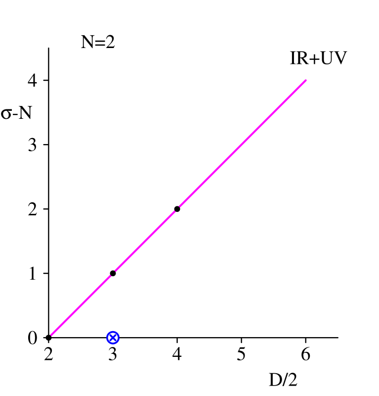
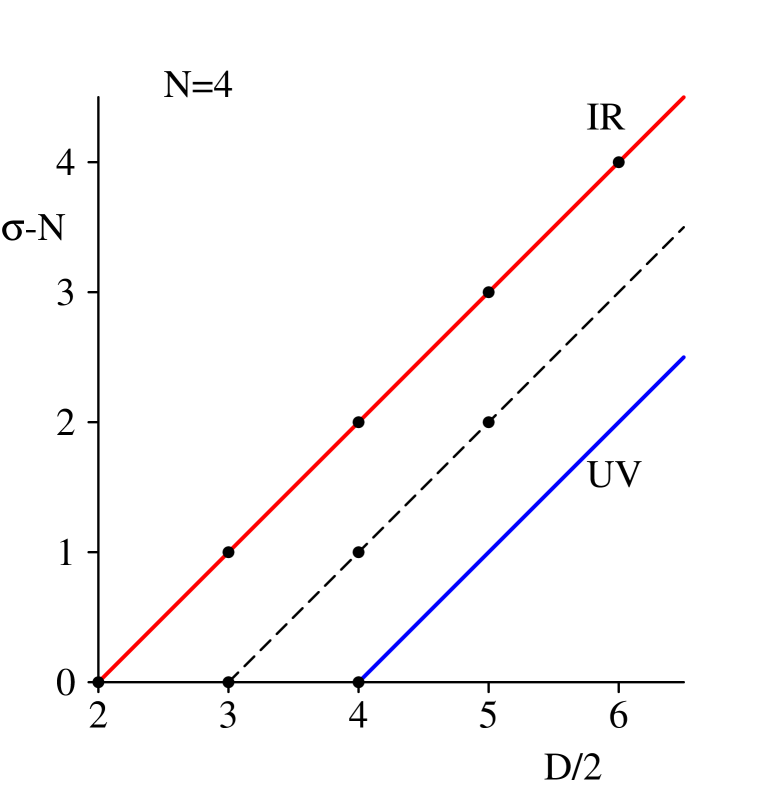
(a) (b)
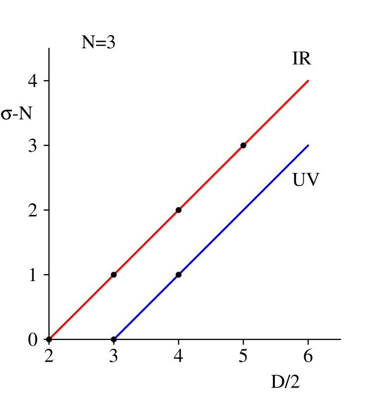
(c) (d)

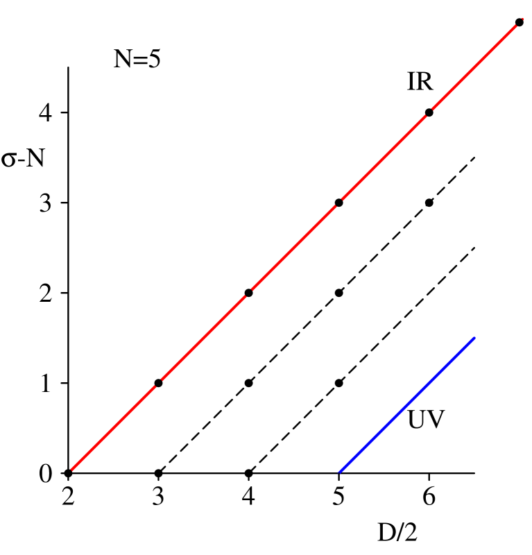
Figure 2: A plot in $(D/2,\sigma)$ for $N=2,3,4,5$. The dots represent integrals that can occur in a Feynman diagram evaluation. The ultraviolet divergent integrals lie along the lower solid line, while the infrared divergences lie along the upper solid line. For $N=2$, the IR and UV divergences coincide and are shown as a magenta line. Finite integrals lie on the dashed lines. The ultraviolet divergent six-dimensional bubble graph (produced by the second rank tensor bubble) is denoted by a blue circle-cross.

First consider how the singularity conditions of Eqs. (10), (11) and (12) work when $\sigma$ and $D$ vary for fixed $N$. This is illustrated in Fig. 2 for $N=2,3,4,5$. In each case, the IR divergent condition of Eq. (10) is shown as a red line, while Eq. (11) is shown as a blue line. For bubble graphs (Fig. 2(a)), the IR and UV lines coincide and are drawn in magenta. The dots represent the integrals that appear when Eq. (4) is applied to tensor integrals up to rank $N$. In all cases, the IR line passes through origin, $\sigma=N$ and $D=4$, indicating that the $D=4$ scalar integral may be IR divergent. We also see that the allowed triangle integrals are always either IR divergent (unless the legs are all off-shell) or UV divergent. On the other hand, for $N\geq 4$, families of finite integrals appear starting with the scalar integral in $D=6$.

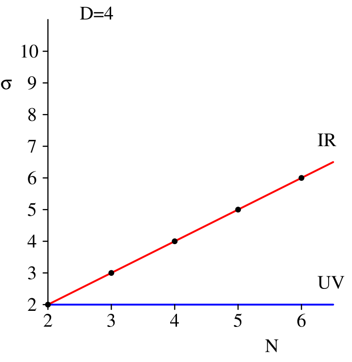
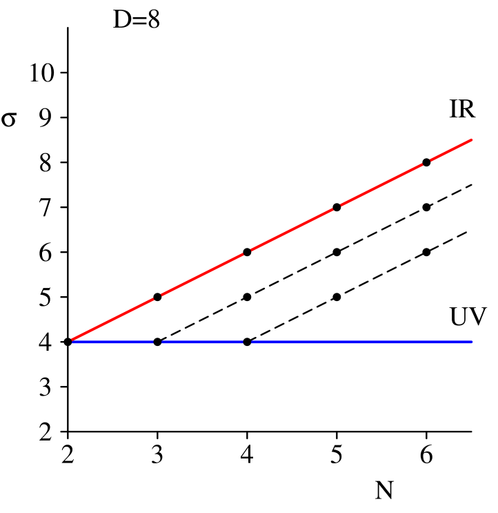
(a) (b)
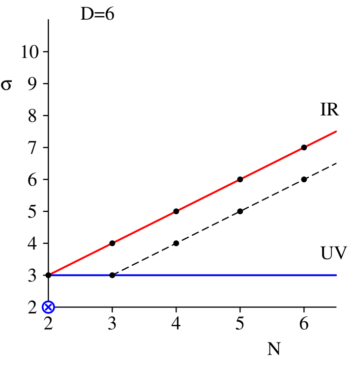
(c) (d)

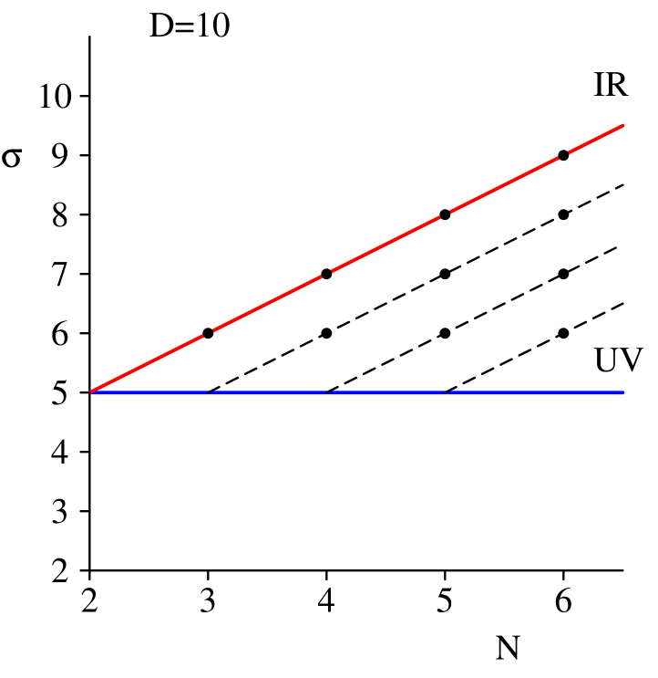
Figure 3: A plot in $(N,\sigma)$ for $D=4,6,8,10$. The dots represent integrals that can occur in a Feynman diagram evaluation. The ultraviolet divergent integrals lie along the blue horizontal line, while the infrared divergences lie along the red line. Finite integrals lie on the dashed lines. The ultraviolet divergent six-dimensional bubble graph (produced by the second rank tensor bubble) is denoted by a blue circle-cross.

It is also instructive to consider the finiteness of integrals of varying $N$ with fixed dimension. This is shown in Fig. 3 where the IR and UV conditions are again shown red and blue while the dots correspond to integrals produced by Eq. (4). Fig. 3(a) shows that all four-dimensional integrals can be divergent while the first integrals that are guaranteed to be finite independent of whether the legs are on-shell or not are higher dimension box graphs.

Reading off the allowed UV divergent integrals from Fig. 3, we see that a suitable (but overcomplete) basis set is

$${\cal I}^{UV} = \left\{I_{4}(D=8-2\epsilon;1,1,1,1),I_{3}(D=8-2\epsilon;2,1,1),I_{2}(D=8-2\epsilon;3,1),\right.$$ (13)

$$\left.I_{2}(D=8-2\epsilon;2,2),I_{3}(D=6-2\epsilon;1,1,1),I_{2}(D=6-2\epsilon;2,1),\right.$$

$$\left.I_{2}(D=6-2\epsilon;1,1),I_{2}(D=4-2\epsilon;1,1)\right\}$$

such that

$${\cal A}_{M}(p_{1},p_{2},\ldots,p_{M})=\sum_{i}K_{i}^{IR}{\cal I}^{IR}_{i}(\{q_{j}\})+\sum_{i}K_{i}^{fin}{\cal I}^{fin}_{i}(\{q_{j}\})+\sum_{i=1}^{8}K_{i}^{UV}{\cal I}_{i}^{UV}(\{q_{j}\}).$$ (14)

While the UV divergent functions are all known analytically [14, 29, 30], the basis sets of finite and IR divergent integrals have an infinite number of members. To derive finite basis sets of known integrals for the latter two classes we employ recursion relations.

2.3 Recursion Relations

In this subsection we show how to map the higher dimensional finite and IR divergent integrals onto a basis set of known finite and divergent integrals. This will fully specify Eq. (2.1) and produce the explicit set of master integrals $\{{\cal I}^{UV},{\cal I}^{IR},{\cal I}^{fin}\}$.

Because the external momenta are 4-dimensional, the recursion relations come in two distinct classes that depend on the number of external legs. When the number of legs is five or less, the external momenta form a vector basis for the resulting tensor structure. However, for more than five external lines, the set of external vectors is over-complete and the net result is that the recursion relations change for $N\geq 6$.

First, we introduce some notation and define the symmetric kinematic matrix

$$S_{ij}=(q_{i}-q_{j})^{2}.$$ (15)

By adding a row (or column) over the inverse of the kinematic matrix we make the further definitions (provided the inverse of the kinematic matrix exists),

$$b_{i}=\sum_{j}S^{-1}_{ij},\qquad\qquad B=\sum_{i}b_{i}=\sum_{ij}S^{-1}_{ij}.$$ (16)

The Gram matrix

$$G_{ij}=2q_{i}\cdot q_{j},$$ (17)

is closely related to the kinematic matrix.

The recursion relations needed to relate all possible integrals to the basis sets are formulated as follows:

I. $N\leq 5$: $\det(S)\neq 0$, $\det(G)\neq 0$

We will use four recursion relations in this case, one basic recursion relation and three derived, composite recursion relations.

The basic recursion relation is obtained by integration by parts as explained in appendix A. It is given by,

$$(\nu_{k}-1)I_{N}(D;\{\nu_{l}\})$$

$$= -\sum_{i=1}^{N}S_{ki}^{-1}I_{N}(D-2;\{\nu_{l}-\delta_{li}-\delta_{lk}\})-b_{k}\left(D-\sigma\right)I_{N}(D;\{\nu_{l}-\delta_{lk}\}),$$

where $\sigma$ is defined in Eq. (7). This relation either reduces both the dimension $D$ and the accompanying value of $\sigma$ by two, or it keeps $D$ fixed and reduces $\sigma$ by one unit. Its action is indicated by the red lines in Fig. 4. This identity is vital for extracting the infrared singularities from the integrals produced by the Davydychev decomposition of Eq. (4).

Note that for the case $N=3$ in Fig. 4(a) we assume that $\det(S)\neq 0$ which is only the case if all three external momenta are off-shell. If any of the external momenta is an on-shell lightcone vector, the inverse of the kinematic matrix does not exist and Eq. (2.3) is invalid. For practical purposes, this is not a problem because analytic expressions for arbitrary dimension and powers of propagators exist for triangle integrals with at least one on-shell leg and massless internal propagators (see Appendix B). In four dimensions, the triangle integral with three off-shell legs and unit propagators is finite and this serves as a reminder that integrals on the “IR” lines in Fig. 4 are not necessarily IR singular, rather they can be IR singular if some of the external momenta are lightlike.

Eq. (2.3) is a more detailed equation than usually quoted in the literature and it can only be applied to scalar integrals with at least one index $\nu_{k}>1$. However, we can use it to derive the standard recursion relation [16],

$$\left(D-1-\sigma\right)\,B\,I_{N}(D;\{\nu_{l}\})=I_{N}(D-2;\{\nu_{l}\})-\sum_{i=1}^{N}b_{i}I_{N}(D-2;\{\nu_{l}-\delta_{li}\}).$$ (19)

Details of the derivation can be found in Appendix A. Eq. (19) reduces $D$ by 2 and $\sigma$ by 1. Its action is illustrated by the blue lines shown in Fig. 4. For the case that all $\nu_{l}=1$ and $D=4-2\epsilon$, we will use this recursion relation to extract the infrared singularities from graphs with at least one on-shell leg as pinched integrals together with scalar integrals in $D=6-2\epsilon$ dimensions,

$$I_{N}(D;\{\nu_{l}\})=\left(D+1-\sigma\right)\,B\,I_{N}(D+2;\{\nu_{l}\})+\sum_{i=1}^{N}b_{i}I_{N}(D;\{\nu_{l}-\delta_{li}\}).$$ (20)

Its action is illustrated by the magenta line in Fig. 4.

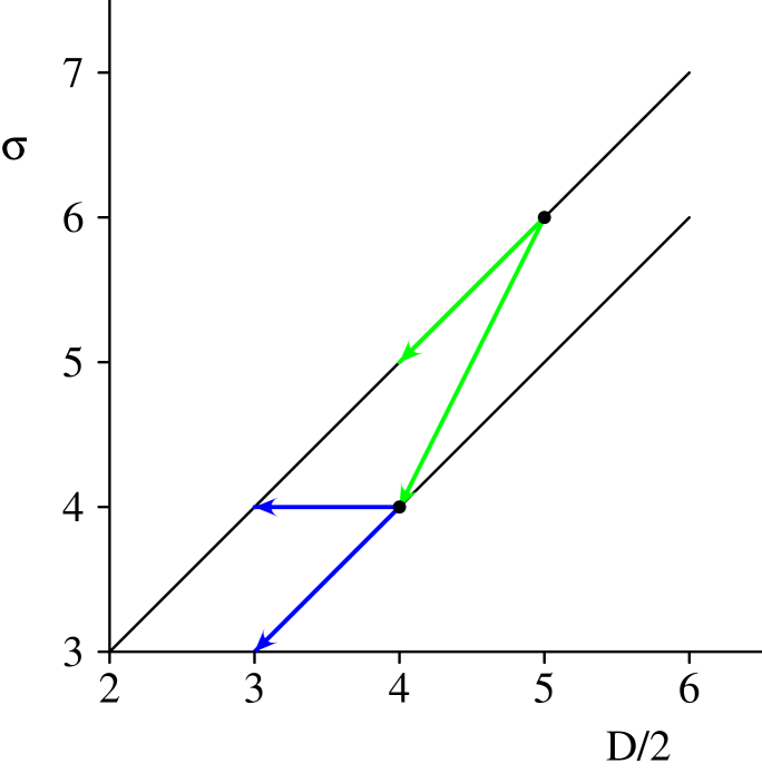
(a) (b)
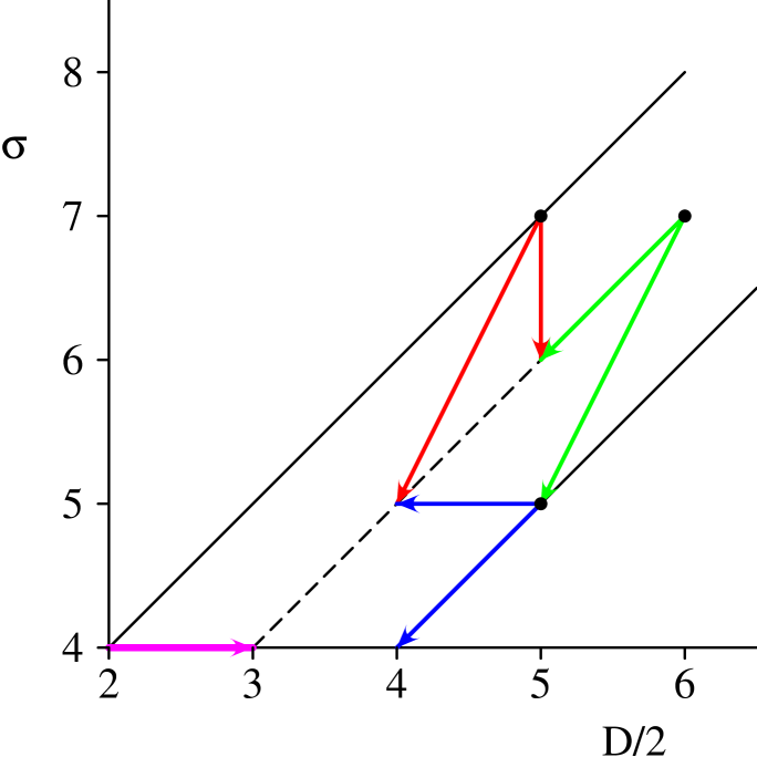
(c)

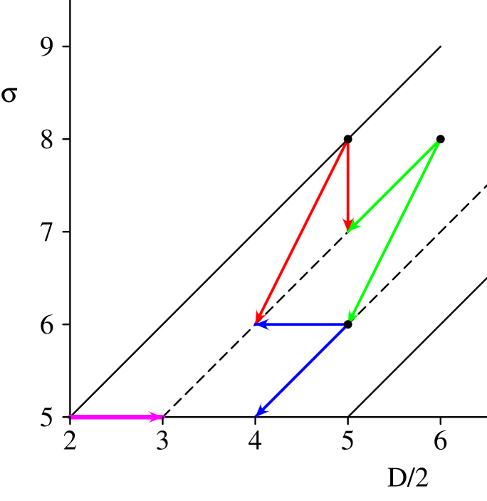
Figure 4: A plot in $(D/2,\sigma)$ for (a) the finite triangle graph, $N=3$, (b) the box graph, $N=4$ and (c) the pentagon graph, $N=5$. The ultraviolet divergent integrals lie along the lower solid line, while for $N>3$ any infrared divergences lie along the upper solid line. Finite integrals lie on the dashed lines. The action of Eqs. (2.3), (19) (20) and (2.3) are shown red, blue, magenta and green respectively.

By combining Eqs. (2.3) and (19) we can eliminate the dimensional prefactor to yield the fourth recursion relation,

$$(\nu_{k}-1)I_{N}(D;\{\nu_{l}\})$$

$$= -\frac{b_{k}}{B}I_{N}(D-2;\{\nu_{l}-\delta_{lk}\})+\sum_{i=1}^{N}\left(\frac{b_{k}b_{i}}{B}-S_{ki}^{-1}\right)I_{N}(D-2;\{\nu_{l}-\delta_{li}-\delta_{lk}\}).$$

This identity reduces $D$ by 2 and $\sigma$ by either 1 or 2 units and its action is indicated in Fig. 4 by the green lines.

When $N=5$ it is easy to avoid the UV line because of the presence of two types of finite integrals ($D/2=\sigma-1$ and $D/2=\sigma-2$). However, this is not the case for $N=3$ and $N=4$ and we are forced to use Eq. (2.3) which appears to produce UV divergent integrals from finite integrals. This implies that in the sum over the produced UV divergent integrals the divergences must cancel. Indeed, because

$$\sum_{i=1}^{N}\left(\frac{b_{k}b_{i}}{B}-S^{-1}_{ki}\right)=0$$

these artificial UV divergences in the individual integrals cancel in the sum as expected. This means we replace each UV divergent integral in Eq. (2.3) by a UV finite regulated integral,

$$\tilde{I}_{N}^{UV}(D=2\sigma;\{\nu_{l}\})=I_{N}^{UV}(D=2\sigma;\{\nu_{l}\})-R(D,\sigma),$$ (22)

where the scaleless regulator term depends on the dimension and $\sigma$ with the constraint $D=2\sigma$,

$$R(D,\sigma)=\frac{1}{\epsilon}\frac{(-1)^{\sigma}}{\Gamma(D-\sigma)}.$$ (23)

After the subtraction the integral is rendered finite. Of course, for this replacement to be useful we must require that Eq. (19) is still valid for the regulated integrals $\tilde{I}_{N}$. Therefore, the regulator function must obey

$$\left(D-1-\sigma\right)\,B\,R(D,\sigma)=-\sum_{i=1}^{N}b_{i}R(D-2,\sigma),$$ (24)

or equivalently

$$\left(D-\sigma-1\right)R(D,\sigma)=-R(D-2,\sigma),$$ (25)

which is trivially verified.

The application of the various recursion relations is clear from the figures:

• If $N\neq 3$ and $D=4$ apply Eq. (20) (magenta arrow)

• If $N\neq 3$ and integral is on the IR line ($D/2=\sigma-N+2$) apply Eq. (2.3) (red arrows)

• In the other cases one can apply Eqs. (19) (blue arrows) and (2.3) (green arrows) with the restriction $\sigma-N+2<D/2\leq\sigma$. Any “fake” UV divergent integrals generated can be regulated as explained in the previous paragraph.

These simple rules are sufficient to reduce all integrals with $N\leq 5$ and non-exceptional kinematics to the basis set of integrals.

II. $N=6$: $\det(S)\neq 0$, $\det(G)=0$

For $N=6$ the kinematic matrix $S_{ij}$ is still invertible. This means that the same recursion relations hold as in the $N<6$ case. However, because $\det(G)=0$, $B=\sum_{i}b_{i}=0$ [16]. This does not affect the basic recursion relation given in Eq. (2.3), but does alter the composite recursion relations and Eqs. (19)–(2.3) all collapse to yield

$$I_{6}(D;\{\nu_{l}\})=\sum_{i=1}^{6}b_{i}I_{6}(D;\{\nu_{l}-\delta_{li}\})\ .$$ (26)

This equation preserves the value of $D$, but reduces $\sigma$ by unity. Its action is indicated by the green arrow in Fig. 5. An additional equation that reduces $D$ is also required and can be obtained by combining Eqs. (2.3) and (26),

$$b_{k}(D-\sigma+\nu_{k}-1)\,I_{6}(D;\{\nu_{l}\})=$$ (27)

$$-\nu_{k}\sum_{i\neq k}^{6}b_{i}I_{6}(D;\{\nu_{l}+\delta_{lk}-\delta_{li}\})-\sum_{i=1}^{6}S_{ki}^{-1}I_{6}(D-2;\{\nu_{l}-\delta_{li}\}).$$

This recursion relation works in 2 different manners. The second term reduces $D$ by 2 and $\sigma$ by unity and acts in a similar manner to the identities for $N\leq 5$ case and is illustrated by the magenta arrow in Fig. 5. On the other hand, the first term preserves both $D$ and $\sigma$ while reducing $N$.

The application of the recursion relations for this case are straightforward.

• If $N=\sigma$ apply Eq. (26).

• If $D/2=\sigma-N+2$ (i.e. on the IR line) apply Eq. (2.3) (red arrow).

• If $D/2<\sigma-1$ apply Eq. (26) or (2.3) (green or red arrow).

• If $D/2=\sigma-1$ apply Eq. (27) (magenta line). The index $k$ is chosen such that $\nu_{k}=\max_{l}(\nu_{l})$ (this is not necessarily a unique choice).

These simple rules are sufficient to reduce all integrals with $N=6$ and non-exceptional kinematics to $N=5$ integrals.

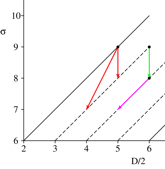
Figure 5: A plot in $(D/2,\sigma)$ for hexagon graphs, $N=6$. The ultraviolet divergent integrals lie along the lower solid line, while the infrared divergences lie along the upper solid line. Finite integrals lie on the dashed lines. The action of Eqs. (2.3), (26) and (27) are shown red, green and magenta respectively. Note that integrals produced by pinching so that $N<6$ are not shown.

III. $N\geq 7$: $\det(S)=0$, $\det(G)=0$

In this case, the inverse of the kinematic matrix does not exist. This invalidates the use of Eqs. (2.3)–(2.3) for $N\geq 7$.

However, the fact that the kinematic matrix is made up of 4-dimensional vectors which obey momentum conservation leads to additional relations. To derive these new types of recursion relations valid for these high values of $N$, we use a generalized inverse based on the singular value decomposition of the Gram matrix.

The first basic recursion relation is based on the kernel of $S$. By solving $(S.z)_{i}=0$ for $z$ we obtain [22]

$$z_{k}\,I_{N}(D;\{\nu_{l}\})=-\sum_{i\neq k}z_{i}I_{N}(D;\{\nu_{l}+\delta_{lk}-\delta_{li}\}),$$ (28)

or alternatively,

$$\sum_{i}z_{i}I_{N}(D;\{\nu_{l}+\delta_{lk}-\delta_{li}\})=0,$$ (29)

where the explicit $z_{i}$ are given in Appendix A. An important property is that $\sum_{i}z_{i}=0$. Eq. (28) keeps $D$ and $\sigma$ constant, but can pinch out particular propagators to reduce $N$. Its effect is illustrated by the magenta arrows in Fig. 6.

The existence of the second recursion relation is highly non-trivial. It is based on the fact that the unit vector $I_{i}=(1,1,\ldots,1)$ lies in the range of the singular matrix $S$, i.e. the equation $(S.r)_{i}=I_{i}$ has a solution for $r_{i}$. The existence of the solution and the explicit construction of the vector $r_{i}$ are detailed in Appendix A and leads to [22]

$$I_{N}(D;\{\nu_{l}\})=\sum_{i}r_{i}I_{N}(D;\{\nu_{l}-\delta_{li}\})$$ (30)

where $\sum_{i}r_{i}=0$. While in functional form this recursion relation is equivalent to Eq. (26), its origin is rather different. This is reflected in the fact that the unique coefficients $b_{i}=\sum_{j}S_{ij}^{-1}$ are unrelated to the many possible and equivalent sets of $r_{i}$ coefficients. For example, replacing $r_{i}\rightarrow r_{i}+\alpha z_{i}$ leaves Eq. (30) unaltered. Eq. (30) also preserves $D$, but reduces $\sigma$ (and possibly $N$) by unity as illustrated by the cyan lines in Fig. 6.

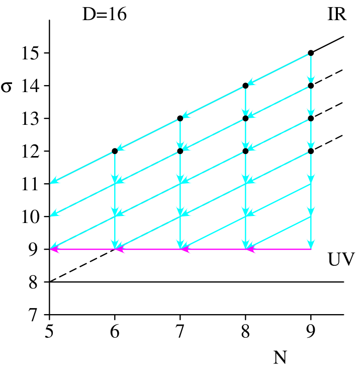
Figure 6: A plot in $(N,\sigma)$ for $D=16$ illustrating the procedure for evaluating integrals with $N\geq 6$. The dots represent the integrals produced in the Davydychev decomposition of rank 6, 7, 8 and 9 tensor integrals. The ultraviolet divergent integrals lie along the lower solid blue line, while the infrared divergences lie along the upper solid red line. The action of Eq. (28) and Eq. (30) are shown as magenta and cyan respectively.

The application of the recursion relations for this case are similar to the $N=6$ case:

• If $N=\sigma$ use Eq. (30)

• If $D/2<\sigma-1$ apply Eq. (30) (cyan arrows).

• If $D/2=\sigma-1$ apply Eq. (28) (magenta line). The index $k$ is chosen such that $\nu_{k}=\max_{l}(\nu_{l})$ (this is not necessarily a unique choice).

These simple rules are sufficient to reduce all integrals with $N\geq 7$ and non-exceptional kinematics to $N=6$ integrals.

2.4 The basis set of integrals

The net result of applying the recursion relations is that any amplitude can be written as,

$${\cal A}_{M}(p_{1},p_{2},\ldots,p_{M}) = \sum_{\nu_{1}\nu_{2}\nu_{3}}K_{\nu_{1}\nu_{2}\nu_{3}}^{IR}I_{3}^{IR}(D=2(\sigma-1);\nu_{1},\nu_{2},\nu_{3})$$ (31)

$$+ \sum_{\{\nu_{\ell}\}}K_{\{\nu_{\ell}\}}^{fin}\tilde{I}_{N}^{UV}(D=2\sigma;\{\nu_{\ell}\})$$

$$+ \sum_{\rm triangles}K_{3}^{fin}I_{3}^{fin}(D=4;1,1,1)$$

$$+ \sum_{\rm boxes}K_{4}^{fin}I_{4}^{fin}(D=6;1,1,1,1)$$

$$+ \sum_{\rm pentagons}K_{5}^{fin}I_{5}^{fin}(D=6;1,1,1,1,1)$$

$$+ \sum_{i=1}^{8}K_{i}^{UV}{\cal I}_{i}^{UV}.$$

Note that the absence of new basis integrals for $N\geq 6$ is intimately related to the dimensionality of space-time (i.e. $\det(G)=0$ for $N\geq 6$). All of the integrals appearing in this basis set are analytically known. The IR and UV divergent integrals with massless internal propagators are known analytically for arbitrary powers of the propagators and arbitrary dimensions [29, 30]. For the sake of completeness, we list them in the Appendix B. Note that the regulated UV divergent triangles $\tilde{I}_{3}^{UV}$ are produced by the action of Eqs. (2.3) and (26) and the sum is therefore finite.

As can be seen in Fig. 2, UV divergent integrals occur for 2-point, 3-point and 4-point functions. By applying Eq. (19) to UV divergent 4-point functions, the UV divergences are moved to 3-point functions. This means the UV basis set of Eq. (13) is reduced to only 2-point and 3-point functions. Analytic formulae for these UV divergent integrals are listed in Appendix B.

The finite 4-dimensional triangle integral with off-shell legs, $I_{3}^{fin}$, and the 6-dimensional box graphs are also known in terms of logarithms and dilogarithms [14, 29]. Furthermore, it is an empirical fact that in final expressions for physical quantities, the 6-dimensional pentagons do not appear [14, 16, 22]. This means $K_{5}^{fin}={\cal O}(\epsilon)$ and we do not need to know $I_{5}(D=6;1,1,1,1,1)$ for NLO calculations.

3 Determining the Infrared Divergent Contributions

In this section we derive the techniques for determining the coefficients $K^{IR}$ that multiply IR divergent triangles $I_{3}^{IR}$ in Eq. (31). All of the other coefficients that multiply the finite integrals can be determined numerically using the recursion relations. However, because the coefficient $K^{IR}$ multiplies a divergent integral, we need to know it in $D$ dimensions. This can only be achieved using analytic methods. In Sec. 3.1, we decompose the divergent part of a rank-$m$ $N$-point function into a sum of tensor structures multiplied by the divergent triangles and a kinematic factor, $C_{N}^{12,j}$. This kinematic factor is the building block for the coefficient $K^{IR}$.

First we derive an analytic expression for $C_{N}^{12,j}$ in Sec. 3.1.4. As it turns out this coefficient does not depend on the rank of its parent integral and all the tensor information is carried by a kinematic Lorentz structures.

While in this section we consider only massless internal lines, the generalization to include masses is straightforward and has been outlined in Ref. [27]. By combining results from [27] with the techniques to deal with tensor integrals explained in this section, one readily obtains the extension to the massive case.

3.1 Derivation of the Divergent Coefficients

As we saw in Sec. 2, the IR divergences of any (tensor) loop integral can be isolated as a combination of triangle integrals with one and two light-like legs [16, 31]. In the standard approach using the recursion relations, the IR divergent graphs are produced from many different sources and ultimately drop out at the end of a lengthy algebraic calculation, often after large cancellations between terms. Here it is our aim to calculate the kinematic coefficients multiplying these infrared divergent integrals ab initio without recourse to the recursion relations. In other words, starting with some given (tensor) loop integral, we would like to take the IR limit directly and isolate the singularities,

$$I_{N}^{\mu_{1}\cdots\mu_{m}}(D;\nu_{1},\ldots\nu_{N}) \stackrel{{\scriptstyle{\rm IR~{}limit}}}{{\longrightarrow}} S_{N}^{\mu_{1}\cdots\mu_{m}},$$ (32)

where $S_{N}$ contains all the infrared singularities. Ultimately, this will produce exactly the correct coefficients $K^{IR}_{\nu_{1}\nu_{2}\nu_{3}}$ that would be produced by application of the recursion relations so that

$${\cal A}_{M}^{IR}(p_{1},p_{2},\ldots,p_{M}) = \sum_{G}\sum_{m=0}^{N}{\cal C}^{G}_{\mu_{1}\mu_{2}\cdots\mu_{m}}S_{N}^{\mu_{1}\cdots\mu_{m}}$$ (33)

$$\equiv \sum_{\nu_{1}\nu_{2}\nu_{3}}K^{IR}_{\nu_{1}\nu_{2}\nu_{3}}I_{3}^{IR}(D=2(\sigma-1);\nu_{1},\nu_{2},\nu_{3}).$$

As we will show, identifying $S_{N}^{\mu_{1}\cdots\mu_{m}}$ is straightforward for scalar integrals but is slightly more involved for tensor integrals.

3.1.1 Scalar Integrals

The infrared singularity corresponds to the limit where the incoming loop momentum at the vertex where particle $i$ joins the graph becomes collinear with the incoming momentum $p_{i}$. If we define $\ell_{i}=\ell+p_{1}+\cdots+p_{i-1}$ ($\ell_{1}=\ell$) to be the momentum entering the vertex and $\ell_{i}+p_{i}$ to be the momentum exiting the vertex, then the collinear limit occurs when $\ell_{i}\rightarrow xp_{i}$. Both propagators adjacent to the incoming momentum $p_{i}$ are now on-shell, $\ell_{i}^{2}=x^{2}p_{i}^{2}=0$ and $(\ell_{i}+p_{i})^{2}\to(1+x)^{2}p_{i}^{2}=0$, and produce infrared singularities. We therefore can construct a term that matches all of the infrared singularities when the loop momentum becomes collinear with one of the external momenta. With the identification $d_{N}=d_{0}$ the counterterm for a scalar $N$-point function in the limit $\ell_{2}\rightarrow xp_{2}$ is given by

$${\cal S}_{N,2}=\Delta(p_{2}^{2})\int\frac{d^{D}\ell}{i\pi^{D/2}}\frac{1}{d_{1}d_{2}}~{}\left[\frac{1}{d_{3}(x)d_{4}(x)\cdots d_{N}(x)}\right]_{\ell_{2}\rightarrow xp_{2}}.$$ (34)

where $\Delta(p_{2}^{2})=1$ when $p_{2}^{2}=0$ and zero otherwise (i.e. when $p_{2}$ is off-shell). The square bracket is to be evaluated in the limit that $\ell_{2}\rightarrow xp_{2}$, or equivalently $\ell\rightarrow xq_{2}-(1+x)q_{1}$. So far, the value of $x$ has not been determined. However, there are still singularities when $x$ takes on the specific value $x=x_{j}$ such that $d_{j}(x_{j})=0$. These singularities can be extracted one at a time so that,

$${\cal S}_{N,2}=\Delta(p_{2}^{2})\sum_{j=3}^{N}\,{\cal D}_{12,j}(1,1,1)~{}\,{\cal C}_{N}^{12,j},$$ (35)

where,

$$\,{\cal D}_{12,j}(1,1,1)=I_{3}(D=4-2\epsilon;\{q_{1},q_{2},q_{j}\},1,1,1)\equiv\int\frac{d^{D}\ell}{i\pi^{D/2}}\frac{1}{d_{1}d_{2}d_{j}}$$ (36)

is independent of the number of legs in the graph. The kinematic factor is given by,

$$\,{\cal C}_{N}^{12,j}=\frac{1}{\prod_{\stackrel{{\scriptstyle i=3}}{{i\neq j}}}^{N}d_{i}(x_{j})}\ .$$ (37)

We now have accomplished our aim for the scalar integral. The IR singularities associated with incoming light-like momentum $p_{2}$ is a sum of kinematic factors multiplying scalar three-point master integrals.

3.1.2 Tensor Integrals

In the case of tensor integrals the derivation is a bit more complicated. In the collinear limit $\ell_{2}\rightarrow xp_{2}$ we find

$${\cal S}_{N,2}^{\mu_{1}\cdots\mu_{m}}=\Delta(p_{2}^{2})\int\frac{d^{D}\ell}{i\pi^{D/2}}\left.\frac{\ell^{\mu_{1}}\cdots\ell^{\mu_{m_{3}}}}{d_{1}d_{2}}~{}\left[\frac{\ell^{\mu_{m_{3}+1}}\cdots\ell^{\mu_{k}}}{d_{3}(x)d_{4}(x)\cdots d_{N}(x)}\right]_{\ell_{2}\rightarrow xp_{2}}\right|_{\mbox{IR limit}}$$ (38)

where $m_{3}$ of the $m$ loop momenta are integrated over and the remaining $(m-m_{3})$ are evaluated in the IR limit $\ell_{2}\rightarrow xp_{2}$. A priori, any value of $m_{3}$ between 0 and $m$ is possible and leads to the correct IR behaviour. In Ref. [27] it is proposed that $m_{3}$ is chosen to be equal to $m$. Using the recursion relations of Sec. 2 this particular choice would give a rather complicated structure of IR triangles. However, as explained above more generic choices for the tensor structure or the IR terms are possible.

To decide on the appropriate partition of loop momenta, it is important to consider the structure of the IR triangles produced by the recursion relations of Sec. 2.3. Once we can get the correct correspondence between the two different methods for evaluating the IR contributions we have by principle of consistency found the right procedure for partitioning the loop momenta.

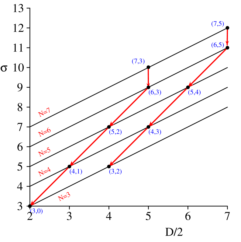
Figure 7: A plot in $(D/2,\sigma)$ showing how the IR divergences from high-rank $N$-point integrals are mapped onto IR divergent triangle integrals using Eqs. (2.3) and (30). The solid lines show the IR trajectories for $N=3,\ldots,7$. The points labelled $(N,m)$ correspond to integrals produced by rank-$m$ $N$-point tensor integrals. The red arrows show how Eqs. (2.3) and (30) systematically reduce both $N$ and $\sigma$ until the integral ends on the $N=3$ IR line.

Fig. 7 shows how the IR divergences from rank-$m$ $N$-point integrals are mapped onto IR divergent triangle integrals using Eqs. (2.3) and (30). Because the recursion relations change in a fundamental matter once $N\geq 7$ we have to distinguish these two cases.

For $N\leq 6$, systematic application of identity  (2.3) reduce both $\sigma$ and $D$ in such a way that the integral jumps from the $N$-point IR trajectory to the $(N-1)$-point IR trajectory. Each jump reduces $\sigma$ by 2 and $D/2$ by unity. Repeated application of the identity will always end on the $N=3$ IR line. Provided that the rank-$m$ satisfies $m\leq N-3$, then we obtain triangle integrals with $\sigma=3$. However, if $m>N-3$, then the recursion relations hit the IR triangle line at $\sigma>3$ and $D/2>2$. In Fig. 7 this is illustrated for rank-5 six-point integrals $(6,5)$. After reduction, we are left with triangle integrals in $D/2=4$ and with $\sigma=5$, precisely the integrals that are produced by rank-2 triangle graphs in $D/2=2$.

For $N\geq 7$ the recursion relation  (30) works rather differently. It keeps $D/2$ fixed, but reduces $\sigma$ and $N$. Repeated application will eventually move the integral onto the $N=6$ IR line and the previous case is applied.

This leads us to the surprisingly simple conclusion that the correct partitioning of loop momenta in Eq. (38). For $N\leq 6$ we find $m_{3}=\max(m+3-N,0)$, while for $N\geq 7$ we have $m_{3}=\max(m-3,0)$. Or summarized in one formula

$$m_{3}=\max(m+3-\min(N,6),0).$$ (39)

When $N\leq 6$ the maximum value of $m_{3}$ is only three (reached for a maximum rank-$m=N$ $N$-point function). However, if $N>6$, the maximum value of $m_{3}$ is $N-3$. Note that only the IR divergent part of the tensor triangle integral is required.

Inserting this value of $m_{3}$ in Eq. (38) and partitioning the loop momenta in a symmetric way the counterterm can be written as

$${\cal S}_{N,2}^{\mu_{1}\cdots\mu_{m}} = \Delta(p_{2}^{2})\sum_{j=3}^{N}\,{\cal C}_{N}^{12,j}{\cal T}^{\mu_{1}\cdots\mu_{m}}_{12,j},$$ (40)

where

$${\cal T}^{\mu_{1}\cdots\mu_{m}}_{12,j}=\,{\cal D}_{12,j}^{[\mu_{1}\cdots\mu_{m_{3}}}{\cal P}_{12,j}^{\mu_{m_{3}+1}\cdots\mu_{m}]}.$$ (41)

The notation

$$A^{\large[\mu_{1}\cdots\mu_{k}}B^{\mu_{k+1}\cdots\mu_{m}\large]}=\sum_{P(\mu_{1}\cdots\mu_{m})}\frac{1}{k!}\frac{1}{(m-k)!}A^{\mu_{1}\cdots\mu_{k}}B^{\mu_{k+1}\cdots\mu_{m}}$$ (42)

shows how the Lorentz indices are distributed between the terms and includes a sum over all permutations of the indices. The kinematic factor $\,{\cal C}_{N}^{12,j}$ is defined in Eq. (37) while the tensor structure remaining in the IR limit is given by,

$${\cal P}_{12,j}^{\nu_{1}\cdots\nu_{k}} = \left[\ell^{\nu_{1}}\cdots\ell^{\nu_{k}}\right]_{\ell\rightarrow x_{j}p_{2}-p_{1}}.$$ (43)

Finally the IR part of the rank-$k$ triangle function is given by,

$$\,{\cal D}_{12,j}^{\nu_{1}\cdots\nu_{k}}=\sum_{x_{1}x_{2}}\left(q_{1}^{x_{1}}q_{2}^{x_{2}}q_{j}^{k-x_{1}-x_{2}}\right)^{\nu_{1}\cdots\nu_{k}}$$ (44)

$$\times I_{3}^{IR}(D=4+k-2\epsilon;q_{1},q_{2},q_{j},x_{1}+1,x_{2}+1,k+1-x_{1}-x_{2}).$$

Eq. (40) produces the IR singularities for the rank-$m$ $N$-point integral in the $l_{2}\rightarrow xp_{2}$ limit. Note that only those 3-point functions which are divergent (i.e. have at least one massless on-shell leg) are kept.

We see that Eq. (40) contains exactly the same IR triangles as would be obtained by using the formalism of Sec. 2 to a rank-$m$ $N$-point function followed by application of the recursion relations. Therefore, by inspection, the divergences of the Eq. (40) are identical to the original tensor integral. Because the kinematic factor $\,{\cal C}_{N}^{12,j}$ does not contain any dimensional term (i.e. does not depend on the regulator $\epsilon$), the finite parts will also match exactly and,

$$\lim_{l_{2}\rightarrow xp_{2}}\left[I_{N}^{\mu_{1}\cdots\mu_{m}}-S_{N,2}^{\mu_{1}\cdots\mu_{m}}\right]\equiv 0.$$ (45)

3.1.3 Sum over all IR limits

We have constructed the IR divergent part of the loop integral associated with the particular limit $\ell_{2}\rightarrow xp_{2}$. Similar IR singular terms for the other cases (i.e. $\ell_{i}\rightarrow xp_{i}$) can be obtained by cyclic permutations of Eq. (35). That is $(\ell_{1},p_{1},d_{1})\rightarrow(\ell_{2},p_{2},d_{2})\rightarrow\cdots\rightarrow(\ell_{N},p_{N},d_{N})\rightarrow(\ell_{1},p_{1},d_{1})$ denoted by $C(12\cdots n)$. However, care has to be taken when adding up all contributions to construct the overall IR singular term. As is well known for real emission soft/collinear divergences, adding up all collinear limits will double count the soft double singularities. The same occurs for the virtual soft poles when two adjacent external momenta are on-shell. For example, when both $p_{2}$ and $p_{3}$ are on-shell we get an identical soft/double pole contribution from ${\cal S}_{n}^{(2)}$ and ${\cal S}_{n}^{(3)}$. These terms are respectively $\,{\cal C}_{n}^{12,3}/d_{1}d_{2}d_{3}$ and $\,{\cal C}_{n}^{23,1}/d_{2}d_{3}d_{1}$. To correct for the double counting we have to subtract this singularity. With this in mind we can now construct the overall IR singular term for the loop integral,

$${\cal S}_{N}^{\mu_{1}\cdots\mu_{m}} = \sum_{C(12\cdots n)}\left[{\cal S}_{N,2}^{\mu_{1}\cdots\mu_{m}}-\Delta(p_{2}^{2})\Delta(p_{3}^{2}){\cal T}_{12,3}^{\mu_{1}\cdots\mu_{m}}\,{\cal C}_{N}^{12,3}\right]$$ (46)

$$= \sum_{C(12\cdots n)}\left[\sum_{j=3}^{n}\Delta(p_{2}^{2}){\cal T}_{12,j}^{\mu_{1}\cdots\mu_{m}}\,{\cal C}_{N}^{12,j}-\Delta(p_{2}^{2})\Delta(p_{3}^{2}){\cal T}_{12,3}^{\mu_{1}\cdots\mu_{m}}\,{\cal C}_{N}^{12,3}\right]$$

$$= \sum_{C(12\cdots N)}\left[\sum_{j=4}^{n-1}\Delta(p_{2}^{2}){\cal T}_{12,j}^{\mu_{1}\cdots\mu_{m}}\,{\cal C}_{N}^{12,j}\right.$$

$$\phantom{=\sum_{C(12\cdots N)}}\left.+\Delta(p_{2}^{2})\Delta(p_{3}^{2}){\cal T}_{12,3}^{\mu_{1}\cdots\mu_{m}}\,{\cal C}_{N}^{12,3}\right.$$

$$\phantom{=\sum_{C(12\cdots n)}}\left.+\Delta(p_{2}^{2})\left(1-\Delta(p_{3}^{2})\right){\cal T}_{12,3}^{\mu_{1}\cdots\mu_{m}}\,{\cal C}_{N}^{12,3}\right.$$

$$\phantom{=\sum_{C(12\cdots N)}}\left.+\Delta(p_{3}^{2})\left(1-\Delta(p_{2}^{2})\right){\cal T}_{23,1}^{\mu_{1}\cdots\mu_{m}}\,{\cal C}_{N}^{23,1}\right].$$

Eq. (46) clearly shows the different contributions. Just as for real emission soft/collinear behavior, there is a double pole soft contribution when two neighboring incoming momenta are on-shell, $\Delta(p_{2}^{2})=\Delta(p_{3}^{2})=1$. If one of the two neighboring incoming lines is off-shell there is a single pole collinear contribution. However, unlike the real emission case, there is an additional single pole contribution from non-adjacent propagators.

3.1.4 Evaluation of $\,{\cal C}_{N}^{12,j}$

If the momentum $p_{2}$ is light-like, then the condition that $\ell_{2}\rightarrow xp_{2}$ means that all of the propagator factors become first order polynomials in $x$. In this case, we can use,

$$\mbox{$\left(\ell_{2}+p_{2}+\cdots+p_{j}\right)^{2}$}\Big{\rfloor}_{\ell_{2}\rightarrow xp_{2}}=(1+x)s_{2\cdots j}-xs_{3\cdots j},=A_{j}(x-x_{j})$$ (47)

with

$$A_{j} = s_{2\cdots j}-s_{3\cdots j},$$ (48)

$$x_{j} = \frac{s_{2\cdots j}}{s_{3\cdots j}-s_{2\cdots j}},$$ (49)

$$s_{k\cdots j} = \mbox{$\left(p_{k}+\cdots+p_{j}\right)^{2}$},$$ (50)

so that

$$\left[{d_{3}(x)d_{4}(x)\cdots d_{N}(x)}\right]_{\ell_{2}\rightarrow xp_{2}}=\prod_{i=3}^{N}A_{i}(x-x_{i}).$$ (51)

The coefficient $\,{\cal C}_{N}^{12,j}$ is merely the residue evaluated at the singular point $x=x_{j}$,

$$\,{\cal C}_{N}^{12,j}=\frac{1}{\prod_{m=3,m\neq j}^{N}A_{m}(x_{j}-x_{m})}.$$ (52)

Inserting the definitions of $A_{i}$ and $x_{i}$ given in Eqs. (48) and (49) we find

$$\,{\cal C}_{N}^{12,j}=\frac{\left(s_{2\cdots j}-s_{3\cdots j}\right)^{N-3}}{\prod_{k=3,k\neq j}^{N}\left(s_{2\cdots j}s_{3\cdots k}-s_{3\cdots j}s_{2\cdots k}\right)}$$ (53)

where $q_{i}=\sum_{j=1}^{i}p_{i}$ such that the formula respects cyclic permutations of the indices. Eq. (53) holds whether or not $p_{j}^{2}=0$.

The special cases associated with neighboring incoming momenta are obtained by setting $j=3$ in Eq. (53) and noting that $s_{3\cdots 3}=p_{3}^{2}$ so that,

$$\,{\cal C}_{N}^{12,3}=\frac{\left(s_{23}-p_{3}^{2}\right)^{N-3}}{\prod_{k=4}^{N}\left(s_{23}s_{3\cdots k}-p_{3}^{2}s_{2\cdots k}\right)},$$ (54)

corresponding to evaluating $\ell\rightarrow x_{3}p_{2}-q_{1}$ with $x_{3}=s_{23}/(s_{23}-p_{3}^{2})$ and $q_{1}=p_{1}$. The companion coefficient is given by making the cyclic momentum permutation, $p_{1}\to p_{2},p_{2}\to p_{3},q_{1}\to q_{2}$ on Eq. (53) so that $s_{2\cdots j}\to s_{3\cdots 1}=p_{2}^{2}$, $s_{3\cdots j}\to s_{4\cdots 1}=s_{23}$,

$$\,{\cal C}_{N}^{23,1}=\frac{\left(s_{23}-p_{2}^{2}\right)^{N-3}}{\prod_{k=4}^{N}\left(s_{23}s_{3\cdots k}-p_{2}^{2}s_{4\cdots k}\right)},$$ (55)

corresponding to $\ell\to x_{1}p_{3}-p_{1}-p_{2}$ with $x_{1}=-p_{2}^{2}/(p_{2}^{2}-s_{23})$.

When $p_{2}^{2}=p_{3}^{2}=0$ the two coefficients become identical

$$\,{\cal C}_{N}^{12,3}\Big{\rfloor}_{p_{2}^{2}=p_{3}^{2}=0}=\,{\cal C}_{N}^{23,1}\Big{\rfloor}_{p_{2}^{2}=p_{3}^{2}=0}=\frac{1}{\prod_{k=4}^{N}s_{3\cdots k}}.$$ (56)

As an application of Eq. (46), in Appendix C we write down an expression for the IR singularities for a scalar massless $N$-point function with all external momenta on-shell.

4 Outlook and Conclusions

The formalism outlined in this paper offers a realistic prospect of constructing NLO Monte Carlo programs for processes involving high multiplicity final state particles. The key result is a strategy for combining the analytic evaluation of the IR and UV singular contributions to loop integrals by using a suitable basis of divergent integrals with a system of recursion relations which allows the numerical determination of the finite integrals. This mixed approach avoids the usual algebraic log-jam in loop calculations that occurs when many particles and kinematic scales are present. In this paper, we have focussed on massless particles circulating in the loop. However, the extension to massive particles is straightforward and opens up the possibility of computing the NLO corrections to any Standard Model process.

The next phase of this project is the actual numerical implementation of the algorithms such that a rank-$m$ $N$-point function can be calculated. There are two avenues of approach. The first approach is to use the recursive algorithms numerically. The advantages are simplicity and all kinematic coefficients are calculated numerically. This allows us to check that e.g $K_{5}=0$ and all $K^{IR}$ can be compared to the analytic calculation of these divergent coefficients. The recursive algorithm is a good diagnostic tool.

However, if the aim is to calculate a full amplitude made up from many graphs containing different integrals of varying rank, the recursive approach would not be optimal. This is because the calculation of a rank-$m$ $N$-point function uses some of the calculations needed for evaluating a rank-$k$ $M$-point function ($k\leq m$, $M\leq N$). To avoid duplicate calculations and irrelevant paths, one could use a constructive method for evaluating the integrals. The algorithm starts by calculating all the relevant finite basis integrals. Then, step by step, we calculate the integrals with higher $D$, $N$ and $\sigma$ using the recursion relations in the reverse sense. For example, assume all $I_{M}(D;\{\nu_{l}\})$ are known with $\sigma\leq s_{0}$ (i.e. each integral is a number in a look-up table). Using the recursion relations of Sec. 2, we can then calculate all the $I_{N}(D;\{\nu_{l}\})$ with $\sigma=s_{0}+1$. Now we know the look-up table for all integrals with $\sigma\leq s_{0}+1$. We continue with this procedure until all integrals with $M\leq N$ are known. After that, building the amplitudes is easy. All the tensor structures from the Davydychev decomposition are contracted in with the tree level currents. We can simply look up the numerical value for the appropriate integral $I_{N}(D;\{\nu_{l}\})$ in the table. This method is very efficient. However, some of the diagnostic tools have been lost. (E.g. we assume $K_{5}=0$ and all divergent coefficients are correct).

Taken together, the combination of recursive numerical and analytic algorithms should provide a compact and efficient way of evaluating multiparticle one-loop amplitudes, thereby opening up the possibility of estimating the NLO QCD corrections for processes such as $pp\rightarrow N$ jets in association with vector-boson(s) or Higgs particles. Or for example, $pp\rightarrow Q\bar{Q}$ plus $N$ jets at NLO, $pp\rightarrow Q_{1}\bar{Q_{1}}\,+\,Q_{2}\bar{Q_{2}}\,$ plus $N$ jets at NLO, etc. The only limiting factor on the particles is that the spin/helicity is less than or equal to one and (numerical) computing power. We expect that this latter problem will be solved with the advent of the LHC Computing Grid.

Appendix A Derivation of Recursion Relations

The one-loop recursion relations are based on the integration by parts techniques developed in Ref. [33] for calculating higher order beta functions. The application to one-loop multi-leg recursion relations was developed in Ref. [12, 22]. Here we will initially follow Ref. [22] by applying the integration by parts identity to

$$\int\frac{d^{D}\ell}{(2\pi)^{D}}\frac{\partial}{\partial\ell^{\mu}}\left(\frac{\left(\sum_{i=1}^{N}y_{i}\right)\ell^{\mu}+\left(\sum_{i=1}^{N}y_{i}q_{i}^{\mu}\right)}{d_{1}^{\nu_{1}}d_{2}^{\nu_{2}}\cdots d_{N}^{\nu_{N}}}\right).$$ (57)

After some trivial algebra and applying the dimensional shift identity

$$I_{N}(D-2;\{\nu_{k}\})=-\sum_{i=1}^{N}\nu_{i}\,I_{N}(D;\{\nu_{k}+\delta_{ik}\})\ ,$$ (58)

one finds the base equation

$$\sum_{j=1}^{N}\left(\sum_{i=1}^{N}S_{ji}y_{i}\right)\nu_{j}I_{N}(D;\{\nu_{l}+\delta_{lj}\})$$ (59)

$$= -\sum_{i=1}^{N}y_{i}I_{N}(D-2;\{\nu_{l}-\delta_{li}\})-\left(D-1-\sum_{j=1}^{N}\nu_{j}\right)\left(\sum_{i=1}^{N}y_{i}\right)I_{N}(D;\{\nu_{l}\})\ ,$$

which is valid for any choice of the $N$ parameters $\{y_{i}\}$.

To reduce tensor integrals in a systematic way, more general recursion relations are needed than those previously given in the literature [12, 22]. For any useful identity, the parameters $\{y_{i}\}$ must be chosen such that the matrix expression $\sum_{i=1}^{N}S_{ji}y_{i}$ is either a delta function, zero or a unit vector. In all these cases, the left hand side of Eq. (59) reduces to a single term thereby yielding a useful recursion relation.

Note that while the recursion relation is expressed in terms of the kinematic matrix $S$, the underlying Gram matrix $G$, also plays an important role. For example, for $N\geq 6$ the Gram determinant vanishes and this has generic consequences for the parameters $\{y_{i}\}$. To understand this we decompose the kinematic matrix. The equation to be solved is [16],

$$\sum_{j=1}^{N}S_{ij}y_{j}=c\times(1,1,\ldots,1)\equiv\sum_{j=1}^{N}\left(\frac{1}{2}G_{ii}y_{j}+\frac{1}{2}G_{jj}y_{j}-G_{ij}y_{j}\right)$$ (60)

for both $c=0$ and $c=1$. In other words,

$$\sum_{j=1}^{N-1}G_{ij}y_{j}=\frac{1}{2}Bw_{i},\qquad\qquad\sum_{j=1}^{N-1}w_{j}y_{j}=c,\qquad\qquad\sum_{j=1}^{N}y_{j}=B$$ (61)

where $w_{i}=\frac{1}{2}G_{ii}$.

Using momentum conservation at the level of the loop integral, we can enforce $B={\rm det}(G)=0$ by setting $y_{N}=-\sum_{j=1}^{N-1}y_{j}$. In fact, this particular choice guarantees that a solution exists and that,

$$\sum_{j=1}^{N-1}G_{ij}y_{j}\equiv 0,\qquad\qquad\sum_{j=1}^{N-1}w_{j}y_{j}=c,\qquad\qquad B=\sum_{j=1}^{N}y_{j}\equiv 0.$$ (62)

Therefore any vector in the kernel of $G$ satisfying $w.y=c$ is a solution of $(S.y)_{i}=c$ for $N\geq 6$.

We can now construct the specific $\{y_{i}\}$ for all the cases specified in sec. 2.3. To do so we apply the Singular Value Decomposition (SVD) technique. Using the decomposition we can explicitly construct the parameters $\{y_{i}\}$ for Eqs. (2.3), (28) and (30). Note that Eq. (19) follows from Eq. (2.3) by summing over index $k$ and applying identity (58). Subsequently, Eq. (2.3) follows by combining Eqs. (19) and (2.3).

The three distinct situations are:

I. $N\leq 6$: $\det(S)\neq 0$, $\sum_{j=1}^{N}S_{ij}b_{j}=\delta_{ik}$

In this case the inverse of the kinematic matrix exists and the range of the matrix covers all of parameter space, specifically the unit vectors.

While many algorithms exist for calculating the inverse, we still use the stable SVD for the kinematic matrix. This gives good control over the numerical accuracy of the matrix inversion which will be important as the external momenta approach exceptional configurations. The SVD is given by

$$S_{ij}=\sum_{k=1}^{N}\omega_{k}u_{ik}v_{kj}^{T},$$ (63)

where the $N$ $\omega_{k}$ are the non-zero eigenvalues of $S$ and the matrices $u$ and $v$ are orthogonal i.e. $(v.v^{T})_{ij}=(u.u^{T})_{ij}=\delta_{ij}$. For an explicit algorithm which calculates both the eigenvalues and the orthogonal matrices see e.g. [34].

For any $k\leq N$, the choice,

$$b_{i}=S_{ik}^{-1}=\sum_{j=1}^{N}\omega_{j}^{-1}v_{ij}u_{jk}^{T},$$ (64)

yields $S_{ij}b_{j}=\delta_{ik}$ which immediately leads to Eq. (2.3). Note that because of Eq. (62), when $N=6$ we find the special identity $B=\sum_{ij}S_{ij}^{-1}=0$, which then leads directly to Eq. (26).

II. $N\geq 7$: $\det(S)=0$, $\sum_{j=1}^{N}S_{ij}z_{j}=0$

In this case the inverse is no longer defined. However for any vector in the kernel of the singular matrix $S$ we have $\sum_{j}S_{ij}z_{j}=0$. By selecting $z_{i}$ with the property $\sum_{i}z_{i}=0$, we find Eq. (28).

To construct this solution,we simply solve Eq. (62) by picking a vector out of the kernel of $G$ such that $w.z=0$ For explicit construction of these vectors we first apply the SVD to the Gram matrix (and not the kinematic matrix),

$$G_{ij}=\sum_{k=1}^{4}\omega_{k}u_{ik}v_{kj}^{T}.$$ (65)

With this decomposition, one of the possible choices for $z_{i}$ is

$$z_{i}=\frac{W_{6}v_{i5}-W_{5}v_{i6}}{W_{5}+W_{6}},$$ (66)

where

$$W_{i}=\frac{1}{2}\sum_{j=1}^{N-1}G_{jj}v_{ji}.$$ (67)

Note that this solutions has the special property $B=\sum_{i=1}^{N}z_{i}=0$ by construction.

III. $N\geq 7$: $\det(S)=0$, $\sum_{j}S_{ij}r_{j}=1$

The fact that the vector $(1,1,\ldots,1)$ is in the range of the singular matrix is a highly non-trivial statement. It is due to the properties of the underlying decay/scattering process. With the property that $\sum_{j}S_{ij}r_{j}=1$ and $\sum_{j}r_{j}=0$ we readily obtain Eq. (30).

By inspecting Eq. (62), we know that a solution exists. We simply pick a vector out of the kernel of $G$ such that $w.r=0$.

A explicit construction of the parameters $r_{i}$ again passes through the SVD of the Gram matrix, Eq. (65). An example of the $r_{i}$ satisfying all of the above requirements is given by,

$$r_{i}=\frac{v_{i5}}{W_{5}}\ .$$ (68)

With these explicit constructions of the solutions for $(b,z,r)$, we have fully specified the recursion relations. The SVD yields, not only an explicit construction of the solution, but also a diagnostics tool for exceptional momentum configurations. These configurations can occur, even in non-singular cases. While integrable, they may require special treatment to maintain numerical accuracy. The SVD is particular useful to identify these situations.

Appendix B Analytic forms for the divergent integrals

The one-loop bubble integral with external momentum scale $Q_{1}^{2}$ with arbitrary powers of massless propagators is given by

$$I_{2}(D;\{\nu_{1},\nu_{2}\})=(-1)^{\sigma}(-Q_{1}^{2})^{\frac{D}{2}-\sigma}\frac{\Gamma\left({\frac{D}{2}-\nu_{1}}\right)\Gamma\left({\frac{D}{2}-\nu_{2}}\right)\Gamma\left({\sigma-\frac{D}{2}}\right)}{\Gamma\left({\nu_{1}}\right)\Gamma\left({\nu_{2}}\right)\Gamma\left({D-\sigma}\right)}$$ (69)

Inserting specific choices for $\{\nu_{1},\nu_{2}\}$, we see that,

$$I_{2}(D=4-2\epsilon;\{1,1\}) = c_{\Gamma}\frac{1}{\epsilon(1-2\epsilon)}\left(-Q_{1}^{2}\right)^{-\epsilon},$$ (70)

$$I_{2}(D=6-2\epsilon;\{1,1\}) = c_{\Gamma}\frac{1}{2\epsilon(1-2\epsilon)(3-2\epsilon)}\left(-Q_{1}^{2}\right)^{1-\epsilon},$$ (71)

$$I_{2}(D=6-2\epsilon;\{2,1\}) = -c_{\Gamma}\frac{1}{2\epsilon(1-2\epsilon)}\left(-Q_{1}^{2}\right)^{-\epsilon},$$ (72)

$$I_{2}(D=8-2\epsilon;\{2,2\}) = c_{\Gamma}\frac{(1-\epsilon)}{2\epsilon(1-2\epsilon)(3-2\epsilon)}\left(-Q_{1}^{2}\right)^{-\epsilon},$$ (73)

$$I_{2}(D=8-2\epsilon;\{3,1\}) = c_{\Gamma}\frac{(2-\epsilon)}{4\epsilon(1-2\epsilon)(3-2\epsilon)}\left(-Q_{1}^{2}\right)^{-\epsilon}.$$ (74)

where

$$c_{\Gamma}=\frac{\Gamma(1-\epsilon)^{2}\Gamma(1+\epsilon)}{\Gamma(1-2\epsilon)}.$$ (75)

The one-loop triangle integral with two on-shell legs, one off-shell external momentum scale $Q_{1}^{2}$ and with arbitrary powers of massless propagators is given by

$$I_{3}(D;\{\nu_{1},\nu_{2},\nu_{3}\})\!\! = \!\!(-1)^{\sigma}(-Q_{1}^{2})^{\frac{D}{2}-\sigma}$$ (76)

$$\times \!\!\frac{\Gamma\left({\frac{D}{2}-\nu_{1}-\nu_{2}}\right)\Gamma\left({\frac{D}{2}-\nu_{1}-\nu_{3}}\right)\Gamma\left({\sigma-\frac{D}{2}}\right)}{\Gamma\left({\nu_{2}}\right)\Gamma\left({\nu_{3}}\right)\Gamma\left({D-\sigma}\right)}.$$

Note that $\nu_{1}$ refers to the propagator opposite the off-shell external leg.

The one-loop triangle integral with one on-shell legs, two off-shell external momentum scales $Q_{1}^{2}>Q_{2}^{2}$ and with arbitrary powers of massless propagators is given by

$$I_{3}(D;\{\nu_{1},\nu_{2},\nu_{3}\})$$ (78)

$$= (-1)^{\sigma}~{}(-Q_{1}^{2})^{\frac{D}{2}-\sigma}\frac{\Gamma\left(\frac{D}{2}-\nu_{1}-\nu_{2}\right)\Gamma(\frac{D}{2}-\nu_{1}-\nu_{3})\Gamma(\sigma-\frac{D}{2})}{\Gamma(\nu_{2})\Gamma(\nu_{3})\Gamma(D-\sigma)}$$

$$\hskip 85.35826pt\times\phantom{~{}}{{}_{2}F_{1}}\left(\nu_{1},\sigma-\frac{D}{2},1+\nu_{1}+\nu_{3}-\frac{D}{2},\frac{Q_{2}^{2}}{Q_{1}^{2}}\right)$$

$$+ (-1)^{\sigma}~{}(-Q_{1}^{2})^{-\nu_{2}}~{}(-Q_{2}^{2})^{\frac{D}{2}-\nu_{1}-\nu_{3}}\frac{\Gamma\left(\frac{D}{2}-\nu_{1}-\nu_{2}\right)\Gamma\left(\frac{D}{2}-\nu_{3}\right)\Gamma\left(\nu_{1}+\nu_{3}-\frac{D}{2}\right)}{\Gamma(\nu_{1})\Gamma(\nu_{3})\Gamma(D-\sigma)}$$

$$\hskip 85.35826pt\times\phantom{~{}}{{}_{2}F_{1}}\left(\nu_{2},\frac{D}{2}-\nu_{3},1+\frac{D}{2}-\nu_{1}-\nu_{3},\frac{Q_{2}^{2}}{Q_{1}^{2}}\right)~{}.\phantom{aaa}$$

Note that $\nu_{3}$ refers to the propagator opposite the on-shell external leg.

Appendix C The scalar $N$-point function

Using Eq. (46) can write down the singular structure for the scalar $N$-point function with all legs on-shell,

$${\cal S}_{N}=\sum_{C(12\cdots N)}\left[-\,{\cal D}_{12,3}\,{\cal C}_{N}^{12,3}+\sum_{j=3}^{N}\,{\cal D}_{12,j}\,{\cal C}_{N}^{12,j}\right].$$ (79)

Integrating out the loop momentum in the scalar triangle integrals yields

$${\cal S}_{N} = c_{\Gamma}\frac{1}{\epsilon^{2}}\sum_{C(12\cdots n)}\left[-\frac{(-s_{23})^{-\epsilon}}{\prod_{k=4}^{N}s_{2\cdots k}}\right.$$ (80)

$$\left.\phantom{}+\sum_{j=3}^{N}\frac{(s_{23\cdots j}-s_{3\cdots j})^{N-4}}{\prod_{k=3,k\neq j}^{N}(s_{23\cdots j}s_{3\cdots k}-s_{3\cdots j}s_{23\cdots k})}\left((-s_{23\cdots j})^{-\epsilon}-(-s_{3\cdots j})^{-\epsilon}\right)\right].$$

This expression agrees with the singular structure singularity structure for the massless six-point function with all momenta on-shell given in Ref. [16] and the corresponding massless five-point function with all momenta on-shell given in Ref. [32] as well as the massless four-point function of Ref. [14].

It is straightforward to use Eq. (46) to check the known singularity structure for massless box graphs with all possible combinations of off-shell conditions for the external momenta given in Ref. [14] as well as the massless pentagon with one off-shell external momenta [32].

References

-
[1]
F. A. Berends and W. T. Giele,
Nucl. Phys. B 306, 759 (1988);
F. A. Berends, W. T. Giele and H. Kuijf, Phys. Lett. B 232, 266 (1989);
F. A. Berends, H. Kuijf, B. Tausk and W. T. Giele, Nucl. Phys. B 357, 32 (1991);
F. Caravaglios and M. Moretti, Phys. Lett. B 358, 332 (1995) [arXiv:hep-ph/9507237];
P. Draggiotis, R. H. Kleiss and C. G. Papadopoulos, Phys. Lett. B 439, 157 (1998) [arXiv:hep-ph/9807207];
P. D. Draggiotis, R. H. Kleiss and C. G. Papadopoulos, Eur. Phys. J. C 24, 447 (2002) [arXiv:hep-ph/0202201];
M. L. Mangano, M. Moretti, F. Piccinini, R. Pittau and A. D. Polosa, JHEP 0307, 001 (2003) [arXiv:hep-ph/0206293]. -
[2]
T. Stelzer and W. F. Long,
Comput. Phys. Commun. 81, 357 (1994)
[arXiv:hep-ph/9401258];
A. Pukhov et al., arXiv:hep-ph/9908288;
F. Yuasa et al., Prog. Theor. Phys. Suppl. 138, 18 (2000) [arXiv:hep-ph/0007053];
F. Krauss, R. Kuhn and G. Soff, JHEP 0202, 044 (2002) [arXiv:hep-ph/0109036]. - [3] E. W. N. Glover, Nucl. Phys. Proc. Suppl. 116, 3 (2003) [arXiv:hep-ph/0211412].
-
[4]
W. B. Kilgore and W. T. Giele,
Phys. Rev. D 55, 7183 (1997)
[arXiv:hep-ph/9610433];
Z. Nagy, Phys. Rev. Lett. 88, 122003 (2002) [arXiv:hep-ph/0110315]. - [5] J. Campbell and R. K. Ellis, Phys. Rev. D 65, 113007 (2002) [arXiv:hep-ph/0202176].
-
[6]
W. Beenakker, S. Dittmaier, M. Kramer, B. Plumper, M. Spira and P. M. Zerwas,
Nucl. Phys. B 653, 151 (2003)
[arXiv:hep-ph/0211352];
S. Dawson, C. Jackson, L. H. Orr, L. Reina and D. Wackeroth, Phys. Rev. D 68, 034022 (2003) [arXiv:hep-ph/0305087]. -
[7]
V. Del Duca, W. Kilgore, C. Oleari, C. Schmidt and D. Zeppenfeld,
Phys. Rev. Lett. 87, 122001 (2001)
[arXiv:hep-ph/0105129];
V. Del Duca, W. Kilgore, C. Oleari, C. Schmidt and D. Zeppenfeld, Nucl. Phys. B 616, 367 (2001) [arXiv:hep-ph/0108030]. -
[8]
E. W. N. Glover and D. J. Miller,
Phys. Lett. B 396, 257 (1997)
[arXiv:hep-ph/9609474];
Z. Bern, L. J. Dixon, D. A. Kosower and S. Weinzierl, Nucl. Phys. B 489, 3 (1997) [arXiv:hep-ph/9610370];
J. M. Campbell, E. W. N. Glover and D. J. Miller, Phys. Lett. B 409, 503 (1997) [arXiv:hep-ph/9706297];
Z. Bern, L. J. Dixon and D. A. Kosower, Nucl. Phys. B 513, 3 (1998) [arXiv:hep-ph/9708239]. - [9] Z. Nagy and Z. Trocsanyi, Phys. Rev. D 59, 014020 (1999) [Erratum-ibid. D 62, 099902 (2000)] [arXiv:hep-ph/9806317].
- [10] Z. Nagy and Z. Trocsanyi, Phys. Rev. Lett. 87, 082001 (2001) [arXiv:hep-ph/0104315].
-
[11]
W. T. Giele and E. W. N. Glover,
Phys. Rev. D 46, 1980 (1992);
S. Catani and M. H. Seymour, Phys. Lett. B 378, 287 (1996) [arXiv:hep-ph/9602277]. -
[12]
D. B. Melrose,
Nuovo Cim. 40, 181 (1965);
W. L. van Neerven and J. A. M. Vermaseren, Phys. Lett. B 137, 241 (1984).
-
[13]
Z. Bern, L. J. Dixon and D. A. Kosower,
Phys. Lett. B 302, 299 (1993)
[Erratum-ibid. B 318, 649 (1993)]
[arXiv:hep-ph/9212308].
-
[14]
Z. Bern, L. J. Dixon and D. A. Kosower,
Nucl. Phys. B 412, 751 (1994)
[arXiv:hep-ph/9306240].
-
[15]
O. V. Tarasov,
Phys. Rev. D 54, 6479 (1996)
[arXiv:hep-th/9606018];
J. M. Campbell, E. W. N. Glover and D. J. Miller, Nucl. Phys. B 498, 397 (1997) [arXiv:hep-ph/9612413];
J. Fleischer, F. Jegerlehner and O. V. Tarasov, Nucl. Phys. B 566, 423 (2000) [arXiv:hep-ph/9907327].
-
[16]
T. Binoth, J. P. Guillet and G. Heinrich,
Nucl. Phys. B 572, 361 (2000)
[arXiv:hep-ph/9911342].
-
[17]
T. Binoth, J. P. Guillet, G. Heinrich and C, Schubert,
Nucl. Phys. B 615, 385 (2001)
[arXiv:hep-ph/0106243].
-
[18]
W. Giele et al.,
arXiv:hep-ph/0204316.
-
[19]
G.J. van Oldenborgh and J.A.M. Vermaseren,
Z. Phys. C 46 425 (1990).
-
[20]
A. Ferroglia, M. Passera, G. Passarino and S. Uccirati,
Nucl. Phys. B 650, 162 (2003)
[arXiv:hep-ph/0209219];
G. Passarino and S. Uccirati, Nucl. Phys. B 629, 97 (2002) [arXiv:hep-ph/0112004];
G. Passarino, Nucl. Phys. B 619, 257 (2001) [arXiv:hep-ph/0108252]. - [21] T. Binoth and G. Heinrich, Nucl. Phys. B 680, 375 (2004) [arXiv:hep-ph/0305234].
- [22] G. Duplancic and B. Nizic, arXiv:hep-ph/0303184.
- [23] Z. Bern, L. J. Dixon, D. C. Dunbar and D. A. Kosower, Nucl. Phys. B 435, 59 (1995) [arXiv:hep-ph/9409265].
-
[24]
D. E. Soper,
Phys. Rev. D 62, 014009 (2000)
[arXiv:hep-ph/9910292];
D. E. Soper, Phys. Rev. D 64, 034018 (2001) [arXiv:hep-ph/0103262]. - [25] Z. Nagy and D. E. Soper, JHEP 0309, 055 (2003) [arXiv:hep-ph/0308127].
- [26] T. Binoth, G. Heinrich and N. Kauer, Nucl. Phys. B 654, 277 (2003) [arXiv:hep-ph/0210023].
- [27] S. Dittmaier, Nucl. Phys. B 675, 447 (2003) [arXiv:hep-ph/0308246].
- [28] A. I. Davydychev, Phys. Lett. B 263, 107 (1991).
-
[29]
E.E. Boos and A.I. Davydychev, Theor. Math. Phys. 89(1991)1052;
see also A.I. Davydychev, J. Math. Phys. 32(1991)1052 and J. Math. Phys. 33,358 (1992). - [30] C. Anastasiou, E. W. N. Glover and C. Oleari, Nucl. Phys. B 572, 307 (2000) [arXiv:hep-ph/9907494].
- [31] T. Kinoshita, J. Math. Phys. 3, 650 (1962).
- [32] Z. Bern, L. J. Dixon and D. A. Kosower, Phys. Lett. B 302, 299 (1993) [Erratum-ibid. B 318, 649 (1993)] [arXiv:hep-ph/9212308].
-
[33]
K. G. Chetyrkin, A. L. Kataev, and F. V. Tkachov,
Nucl. Phys. B 174, 345 (1980);
K. G. Chetyrkin and F. V. Tkachov, Nucl. Phys. B 192, 159 (1981). - [34] Numerical Recipes: The Art of Scientific Computing, University of Cambridge (http://www.nr.com).