Abstract

The decay process $H\rightarrow\gamma\gamma$ is examined in a model-independent way within the effective Lagrangian approach. Contribution of a set of irreducible one-loop diagrams involving $SU(2)\times U(1)$ invariant dimension-six bosonic operators is evaluated explicitly. The calculation is intended to fill a gap that exists in the current literature on the subject.
keywords: electroweak interactions; effective Lagrangians; Higgs decay into two photons.
PACS Nos.: 12.15.-y, 14.80.Bn, 12.60.-i

1 Introduction

The standard model (SM) of fundamental interactions has so far proved to be a very successful theory, at least from the point of view of present-day phenomenology. The most prominent unsolved issue is the mechanism of the electroweak symmetry breaking (EWSB) and a possible existence of the related Higgs scalar sector. Current precision tests of the SM seem to point towards a relatively light Higgs boson, i.e. such that $m_{H}<200\,\text{GeV}$ or so (see e.g. [1]). Needless to say, such an “evidence” is only indirect, as it is based on a successful fit of calculated effects of the relevant closed-loop Feynman graphs to the precision electroweak data. Note also that there is another message from the EWSB sector, which is more general and rather spectacular. For the famous parameter $\rho=m_{W}^{2}/m_{Z}^{2}\cos^{2}\theta_{W}$ (with $m_{W}$ and $m_{Z}$ denoting the vector boson masses and $\theta_{W}$ being the weak mixing angle) the experimental data show that, with great accuracy, $\rho=1$. Such a value is naturally obtained from the Higgs sector with doublet structure, or, more generally, from an EWSB mechanism respecting the custodial $SU(2)$ symmetry [2].

On the other hand, a general opinion prevailing nowadays is that SM cannot be, for various reasons, an ultimate model of particle physics – in other words, it should be understood as an effective theory valid below the energy scale of the order $O(1\,\text{TeV})$ and somewhere above that scale, some kind of new physics is to be expected (for a review, see e.g. [3]). A general framework for describing the effects of the physics beyond SM is an appropriate effective Lagrangian. This incorporates, besides the standard renormalizable interaction terms with dimension four and three, also non-renormalizable higher-dimensional terms involving negative powers of a $\Lambda$, the relevant scale of new physics. Thus, the generic form of such an effective electroweak Lagrangian reads

$$\mathscr{L}_{\text{\it eff}}=\mathscr{L}_{SM}+\sum_{n\geq 5}\sum_{i=1}^{N_{n}}\frac{\alpha_{i}^{(n)}}{\Lambda^{n-4}}\mathcal{O}_{i}^{(n)}.$$ (1)

When constructing such an extension of the SM, gauge invariance under $SU(2)\times U(1)$ is required and, in addition to that, one can make a specific assumption concerning the $\Lambda$. We shall assume that $\Lambda\gg v$, where $v\doteq 246\,\text{GeV}$ is the usual electroweak scale. This corresponds to the so-called “decoupling scenario”, in which the $SU(2)\times U(1)$ symmetry is realized linearly (concerning the terminology, see e.g. [4], [5] and references therein). In particular, this means that the unphysical Goldstone bosons enter via the standard complex $SU(2)$ doublet, along with the elementary Higgs boson field and, generally, the low-energy spectrum is supposed to be identical with that of SM. Explicit representation of the non-renormalizable higher-order terms invariant under $SU(2)\times U(1)$ gauge symmetry can be found in the literature, see in particular [6], [7]. Contributions of the higher-dimensional terms to the amplitudes of low-energy processes are then in fact suppressed by powers of the ratio $v/\Lambda$.

In future experimental searches for the Higgs scalars, the process $H\rightarrow\gamma\gamma$ might play an important role, since a light scalar boson (i.e. that with $m_{H}<2m_{W}$) could be detected through this decay mode at LHC (cf. [8] and references therein). Of course, there is no tree-level coupling $H\gamma\gamma$ within SM: the lowest-dimensional interaction term of this type is necessarily proportional to $HF_{\mu\nu}F^{\mu\nu}$ (where $F_{\mu\nu}$ denotes the electromagnetic field strength) if one is to maintain the electromagnetic gauge invariance. However, such a monomial has obviously dimension five and is therefore non-renormalizable. Consequently, SM yields a calculable (i.e. ultraviolet-finite) result for $H\rightarrow\gamma\gamma$ matrix element at one-loop level and this was obtained long ago [9]. It can also be sensitive to possible effects of the new physics described schematically by the expansion (1) and in current literature there are several papers dealing with this issue (see e.g. [10], [11], [5]); let us remark that contributions of higher-dimensional effective interactions to the inverse process $\gamma\gamma\rightarrow H$ have also been considered previously [12]. Nevertheless, what seems to be still missing, is a one-loop calculation involving a complete set of $SU(2)\times U(1)$ invariant operators that would yield the leading correction (in powers of $1/\Lambda$) to the SM result. Some important steps toward this goal have already been made previously in the papers [10], [11] and [5]. In the present paper we would like to fill a gap that, in our opinion, occurs in the existing treatments. In particular, our effort is concentrated on the part of the calculation that is perhaps most tedious from the technical point of view: we evaluate one-particle irreducible purely bosonic one-loop graphs involving just one insertion of a dimension-six effective interaction vertex from (1), with other ingredients descending from SM. An important consistency check of our computation is the transverse tensor structure of the matrix element – this is achieved, similarly as in the SM case, only when a set of relevant graphs is summed. Thus, the results presented in this paper are of rather technical nature, but we believe that they may prove useful in a future complete calculation based on the $SU(2)\times U(1)$ effective Lagrangian of the type (1).

The paper is organized as follows. In the next section we give a brief summary of the basic SM results for $H\rightarrow\gamma\gamma$. In Section 3, the set of $SU(2)\times U(1)$ bosonic operators with dimension six is shown explicitly and in Section 4 we display the main features of the whole calculation. The results are described in some detail in Section 5 and Section 6 contains their short summary and some concluding remarks. To make the paper self-contained, we have added the Appendix containing the definitions and explicit analytic formulae for the Passarino-Veltman functions that are necessary for the evaluation of loop integrals.

2 Standard Model Results

To begin with, let us reproduce here – for reference purposes – the form of the electroweak SM Lagrangian. In the $U$-gauge it reads (for a concise summary see e.g. [13])

$$\begin{split}\mathscr{L}^{(GWS)}_{int}&=\sum_{f}Q_{f}e\bar{f}\gamma^{\mu}fA_{\mu}+\mathscr{L}_{CC}+\mathscr{L}_{NC}\\ &+ig(W^{0}_{\mu}W^{-}_{\nu}\partial\raisebox{9.0pt}[0.0pt]{$\scriptscriptstyle\leftrightarrow$}^{\mu}W^{+\nu}+W^{-}_{\mu}W^{+}_{\nu}\partial\raisebox{9.0pt}[0.0pt]{$\scriptscriptstyle\leftrightarrow$}^{\mu}W^{0\nu}+W^{+}_{\mu}W^{0}_{\nu}\partial\raisebox{9.0pt}[0.0pt]{$\scriptscriptstyle\leftrightarrow$}^{\mu}W^{-\nu})\\ &-g^{2}\bigl{[}\tfrac{1}{2}(W^{-}\cdot W^{+})^{2}-\tfrac{1}{2}(W^{-})^{2}(W^{+})^{2}+(W^{0})^{2}(W^{-}\cdot W^{+})\\ &\hskip 162.18062pt-(W^{-}\cdot W^{0})(W^{+}\cdot W^{0})\bigr{]}\\ &+gm_{W}W^{-}_{\mu}W^{+\mu}H+\frac{1}{2\cos\theta_{W}}gm_{Z}Z_{\mu}Z^{\mu}H\\ &+\frac{1}{4}g^{2}W^{-}_{\mu}W^{+\mu}H^{2}+\frac{1}{8}\frac{g^{2}}{\cos^{2}\theta_{W}}Z_{\mu}Z^{\mu}H^{2}\\ &-\sum_{f}\frac{1}{2}g\frac{m_{f}}{m_{W}}\bar{f}fH-\frac{1}{4}g\frac{m_{H}^{2}}{m_{W}}H^{3}-\frac{1}{32}g^{2}\frac{m_{H}^{2}}{m_{W}^{2}}H^{4},\end{split}$$ (2)

where we have denoted

$$W^{0}_{\mu}=\cos\theta_{W}Z_{\mu}+\sin\theta_{W}A_{\mu}.$$ (3)

The $\mathscr{L}_{CC}$ and $\mathscr{L}_{NC}$ are the usual symbols for charged and neutral current interactions of fermions with vector fields; an explicit form of these terms will not be needed for our calculations.

As we have already stressed in the Introduction, for obvious dimensional reasons there is no direct tree-level $H\gamma\gamma$ coupling within the SM Lagrangian. The one-loop SM graphs for the decay process $H\rightarrow\gamma\gamma$ are shown in Fig.1.

Figure 1: SM one-loop diagrams for $H\rightarrow\gamma\gamma$. Crossing of the external photon lines is implicit in contributions of the graphs (a) and (c).

Note that at this level, the fermionic part is dominated by the contribution of the heaviest fermion species. Therefore we consider here the top quark loop only.

A straightforward calculation yields the following result for the decay matrix element:

$${\cal M}=(F_{\text{VB}}+F_{\text{top}})\Bigl{(}g^{\alpha\beta}-\frac{2k^{\alpha}p^{\beta}}{m_{H}^{2}}\Bigr{)}\varepsilon^{*}_{\alpha}(p)\varepsilon^{*}_{\beta}(k),$$ (4)

where the “formfactors” $F_{\text{VB}}$ and $F_{\text{top}}$ represent the contributions of the vector boson and top quark loop respectively. These are expressed through

$$F_{\text{VB}} =\frac{3im_{W}}{8\pi^{2}}\bigl{[}1+\frac{m_{H}^{2}}{6m_{W}^{2}}+(2m_{W}^{2}-m_{H}^{2})C_{0}(m_{H}^{2},0,0,m_{W}^{2},m_{W}^{2},m_{W}^{2})\bigr{]}\,,$$ (5)

$$F_{\text{top}} =\frac{-i}{6\pi^{2}}\frac{m_{t}^{2}}{m_{W}}\bigl{[}2+(4m_{t}^{2}-m_{H}^{2})C_{0}(m_{H}^{2},0,0,m_{t}^{2},m_{t}^{2},m_{t}^{2})\bigr{]}\,,$$ (6)

with $C_{0}$ denoting the relevant Passarino-Veltman function (see e.g. [14]); the definitions and explicit analytic formulae for a set of these functions are summarized in the Appendix.

Notice also that in writing the result (4), we have pinpointed the tensorial factor

$$T^{\mu\nu}=g^{\mu\nu}-2m_{H}^{-2}k^{\mu}p^{\nu},$$ (7)

which is transverse with respect to the external photon momenta, i.e.

$$p_{\mu}T^{\mu\nu}=0,\qquad k_{\nu}T^{\mu\nu}=0$$ (8)

as anticipated on the basis of the electromagnetic gauge invariance. The appearance of the transverse tensor structure (7) will serve as an important consistency check also in our subsequent calculations with the effective Lagrangian (1).

Finally, let us add that from the matrix element (4) one obtains the decay width

$$\Gamma_{\text{SM}}(H\rightarrow\gamma\gamma)=\frac{8\pi\alpha^{2}G_{F}}{\sqrt{2}}\frac{m_{W}^{2}}{m_{H}}|F_{\text{top}}+F_{\text{VB}}|^{2}\,,$$ (9)

(cf. [14]).

3 Dimension-Six Effective Operators

Let us now proceed to examine in more detail the effective interaction terms with dimension greater than four, described schematically by the second part of the Lagrangian (1). As noted in the Introduction, we shall restrict ourselves to the dimension-six bosonic operators. Thus, the effective Lagrangian we are going to work with has a general form

$$\mathscr{L}_{\text{\it eff}}=\mathscr{L}_{SM}+\sum_{i}\frac{f_{i}^{(6)}}{\Lambda^{2}}\mathcal{O}_{i}^{(6)}.$$ (10)

For the moment, let us leave aside any discussion of possible “realistic” values of the mass scale $\Lambda$ and coupling constants $f_{i}^{(6)}$ that parameterize the effects of a new physics beyond SM. Here we only give a full list of the operators $O_{i}^{(6)}$ that will be utilized in our calculation. An explicit construction of such a set was studied systematically e.g. in [7]. Assuming that the bosonic sector of our effective low-energy theory contains only the particles $W^{\pm}$, $Z$, $\gamma$ and $H$, and imposing the requirement of $SU(2)\times U(1)$ gauge symmetry together with separate invariance under charge conjugation and parity, one arrives at eleven independent dimension-6 monomials in the relevant field variables, namely

$${\cal O}_{WWW}=\text{Tr}[\hat{W}_{\mu\nu}\hat{W}^{\nu\rho}\hat{W}_{\rho}^{\mu}],$$

$${\cal O}_{WW}=\Phi^{\dagger}\hat{W}_{\mu\nu}\hat{W}^{\mu\nu}\Phi,$$

$${\cal O}_{BW}=\Phi^{\dagger}\hat{B}_{\mu\nu}\hat{W}^{\mu\nu}\Phi,$$

$${\cal O}_{DW}=\text{Tr}\bigl{(}[D_{\mu},\hat{W}_{\nu\rho}][D^{\mu},\hat{W}^{\nu\rho}]\bigr{)},$$

$${\cal O}_{DB}=-\frac{{g^{\prime}}^{2}}{2}\left(\partial_{\mu}B_{\nu\rho}\right)\left(\partial^{\mu}B^{\nu\rho}\right),$$

$${\cal O}_{BB}=\Phi^{\dagger}\hat{B}_{\mu\nu}\hat{B}^{\mu\nu}\Phi,$$

$${\cal O}_{W}=(D_{\mu}\Phi)^{\dagger}\hat{W}^{\mu\nu}(D_{\nu}\Phi),$$

$${\cal O}_{B}=(D_{\mu}\Phi)^{\dagger}\hat{B}^{\mu\nu}(D_{\nu}\Phi),$$

$${\cal O}_{\Phi,1}=\left(D_{\mu}\Phi\right)^{\dagger}\Phi^{\dagger}\Phi\left(D^{\mu}\Phi\right),$$

$${\cal O}_{\Phi,2}=\frac{1}{2}\partial^{\mu}\left(\Phi^{\dagger}\Phi\right)\partial_{\mu}\left(\Phi^{\dagger}\Phi\right),$$

$${\cal O}_{\Phi,3}=\frac{1}{3}\left(\Phi^{\dagger}\Phi\right)^{3}.$$ (11)

Some explanatory remarks concerning the notation employed in (11) are in order here. For convenience, we have introduced the symbols $\hat{B}$ and $\hat{W}$ for vector field variables including the gauge coupling constants:

$$\hat{B}_{\mu\nu}=\frac{1}{2}ig^{\prime}B_{\mu\nu},\hskip 28.45274pt\hat{W}_{\mu\nu}=ig\frac{\sigma^{a}}{2}W^{a}_{\mu\nu},$$ (12)

with $\sigma^{a}$ being the standard Pauli matrices and

$$B_{\mu} =-\sin\theta_{W}Z_{\mu}+\cos\theta_{W}A_{\mu}$$ (13)

$$W^{\mp}_{\mu} =\frac{1}{\sqrt{2}}(W^{1}_{\mu}\pm iW^{2}_{\mu}).$$ (14)

The covariant derivative acting on the isospin doublet $\Phi$ has the form

$$D_{\mu}=\partial_{\mu}+\frac{i}{2}g^{\prime}B_{\mu}+ig\frac{\sigma^{a}}{2}W^{a}_{\mu}.$$ (15)

The Higgs boson field is introduced by means of the $\Phi$ in the usual way; in the $U$-gauge this becomes

$$\Phi=\frac{1}{\sqrt{2}}\begin{pmatrix}0\\ v+H\end{pmatrix}.$$ (16)

4 Contribution to $H\rightarrow\gamma\gamma$ from $\mathscr{L}^{(6)}_{\text{boson}}$

With the basic SM results for the $H\rightarrow\gamma\gamma$ decay amplitude at hand (see (4)-(6)), a natural next goal is to calculate the corresponding leading correction due to the $O(1/\Lambda^{2})$ terms in the effective Lagrangian (10). To this end, we shall consider tree-level and one-loop diagrams, in which a vertex originating in the $\mathcal{L}_{\text{boson}}^{(6)}$ appears exactly once. As we have stated in the Introduction, we are primarily interested in a complete evaluation of the one-particle irreducible one-loop bosonic graphs. Note that for this type of contributions, the transversality expressed by eq. (8) represents a non-trivial criterion of correctness of the whole calculation, as it is achieved only in the sum of all relevant diagrams (in contrast to that, a contribution of any individual reducible diagram is transverse by itself).

Two remarks are in order here. First, the complete calculation would have to include an appropriate renormalization procedure: UV divergent parts of one-loop graphs, evaluated by means of dimensional regularization, should be absorbed into a redefinition of the tree-level coefficients of the effective Lagrangian – in other words, they are to be cancelled by appropriate counterterms, whose structure is determined by the considered Lagrangian (10). In the present paper, we do not implement such a full-fledged renormalization procedure, since we temporarily ignore some contributions that have been studied previously by other authors (for example, contributions due to dimension-six fermionic operators and, in general, contributions of various reducible graphs). We prefer to give here just a separate treatment of the above-mentioned irreducible graphs (as far as we know, these have not been calculated before) and a more complete discussion will be presented elsewhere. For practical purposes, when displaying the results obtained for the diagrams in question (see the next section), we remove the UV divergent parts according to the $\hskip 1.13809pt\overline{\text{MS}}\hskip 1.70717pt$ scheme.

The second remark concerns the structure of the operators (11). Taking into account the $U$-gauge representation of the Higgs doublet (16), one can notice that e.g. the $O_{WW}$ and $O_{BB}$ contain, among other things, also parts proportional to the vector boson kinetic terms (of course, these are obtained simply by replacing the $\Phi$ with its vacuum expectation value). In our calculation, contribution of such bilinear terms will be included in the considered Feynman graphs in a straightforward manner, i.e. as any other dimension-six effective coupling. An alternative approach would consist in incorporating such effects into the renormalization constants of the SM (cf. e.g. [7]). Note that bilinear interaction terms arise also from the other operators (11).

Now, let us describe in more detail the set of Feynman graphs that we are going to calculate. As indicated above, we first take the graphs in Fig. 1 and in each of them replace consecutively a SM vertex with one of those stemming from the $\mathscr{L}_{\text{boson}}^{(6)}$. Similarly, one can make insertions of the $O(1/\Lambda^{2})$ terms into propagators within the SM graphs. In this way, one gets 16 diagrams, including the crossing of external legs. Next, there are several graphs with a new (i.e. not SM-like) topology. These are depicted in Fig. 2 (addition of the crossed diagram to Fig. 2b is tacitly assumed).

Figure 2: Irreducible graphs with other than SM-like topologies. The heavy dot stands for a dimension-six effective vertex

Finally, just for an illustration let us give some examples of reducible graphs. Two such contributions are shown in Fig. 3.

Figure 3: $H\rightarrow\gamma\gamma$: tadpole-type vertex corrections

As we have stated before, we will not evaluate them explicitly (though it would be relatively easy). Let us only make the following remark: Closed loops appearing in Fig. 3 belong to the tadpole-type SM subgraphs, which are known to produce corrections to the Higgs vacuum expectation value $v$. In general, such effects can be described in terms of appropriate running value $v(\mu)$ depending on the relevant renormalization scale. It turns out (cf. [15]) that corrections due to running of the $v$ are rather small and thus, in a complete calculation, one would not make a significant error when using everywhere the basic value $v(m_{W})=246.22\,\text{GeV}$ obtained from the Fermi constant (measured precisely in muon decay).

5 Results and Discussion

Let us now describe the results of our calculation. As we noted above, the matrix element obtained from the considered Feynman diagrams exhibits the desired transverse tensor structure:

$${\cal M}(H\rightarrow\gamma\gamma)=X\Bigl{(}g^{\alpha\beta}-\frac{2k^{\alpha}p^{\beta}}{m_{H}^{2}}\Bigr{)}\varepsilon^{*}_{\alpha}(p)\varepsilon^{*}_{\beta}(k),$$ (17)

where $X$ stands for the relevant formfactor. This can be written, in an obvious notation, as

$$X=e^{2}gF_{\text{SM}}+e^{2}F^{\text{tree}}_{\text{eff}}+e^{2}gF^{\text{loop}}_{\text{eff}}$$ (18)

and the corresponding decay rate is then given by

$$\Gamma(H\rightarrow\gamma\gamma)=\frac{8\pi\alpha^{2}G_{F}}{\sqrt{2}}\frac{m_{W}^{2}}{m_{H}}|F_{\text{SM}}+\frac{1}{g}F^{\text{tree}}_{\text{eff}}+F^{\text{loop}}_{\text{eff}}|^{2}\,.$$ (19)

Since we take into account only bosonic operators in our evaluation of the leading $O(1/\Lambda^{2})$ correction to the SM result, from now on we will also consider only the contribution of bosonic loops within SM – in other words, for the moment we will ignore fermions altogether. Thus, we will set

$$F_{\text{SM}}=F_{\text{VB}}$$ (20)

henceforth (cf. (5)). The contribution of dimension-six operators (11) at the tree level has the following simple form:

$$F^{\text{tree}}_{\text{eff}}=\frac{i}{2}(\frac{f_{BB}}{\Lambda^{2}}-\frac{f_{BW}}{\Lambda^{2}}+\frac{f_{WW}}{\Lambda^{2}})m_{H}^{2}v\,.$$ (21)

The non-trivial part of our calculation is represented by the closed-loop contribution. We have five basic topologies (plus two crossings); in the corresponding diagrams we consider insertions of effective dimension-six operators – both in vertices and as propagator corrections. In total, there are 23 one-loop tensor integrals to be calculated. Obviously, such a calculation is huge: a simple counting indicates that one has to expect tensors made of loop momentum with up to ten indices, schematically

$$\sim\int d^{4}l\;l^{\mu_{1}}\ldots l^{\mu_{10}}\times[\text{denominators}]^{-1},$$

where six $(3\times 2)$ $l^{\mu}$’s come from propagators, one $l^{\mu}$ from SM vertices and three loop momenta descend from an effective vertex. Thus, the algebraic reduction of these expressions to the standard scalar integrals is rather long and tedious. Let us also emphasize that the transversality displayed in eq.(17) is achieved only when all relevant irreducible graphs are summed; among those, only Fig. 2c is transverse by itself.

The main result of this paper is the following formula for the $F^{\text{loop}}_{\text{eff}}$:

$$128m_{W}\pi^{2}F^{\text{loop}}_{\text{eff}}=\\ -8i\Bigl{(}f^{\Lambda}_{\scriptscriptstyle B}-2f^{\Lambda}_{\scriptscriptstyle BW}+f^{\Lambda}_{\scriptscriptstyle W}+3g^{2}(-4f^{\Lambda}_{\scriptscriptstyle DW}+f^{\Lambda}_{\scriptscriptstyle WWW})\Bigr{)}m_{H}^{2}m_{W}^{2}B_{0}(0,m_{W}^{2},m_{W}^{2})\\ -3(f^{\Lambda}_{BB}-f^{\Lambda}_{\scriptscriptstyle BW}+f^{\Lambda}_{\scriptscriptstyle WW})m_{H}^{4}B_{0}(m_{H}^{2},m_{H}^{2},m_{H}^{2})\\ +2\Bigl{\{}m_{H}^{2}\Bigl{(}(f^{\Lambda}_{\scriptscriptstyle B}-2f^{\Lambda}_{\scriptscriptstyle BW}+f^{\Lambda}_{\scriptscriptstyle W})m_{H}^{2}-2(f^{\Lambda}_{\scriptscriptstyle B}-2f^{\Lambda}_{\scriptscriptstyle BW}+f^{\Lambda}_{\scriptscriptstyle W}\\ +12g^{2}(-4f^{\Lambda}_{\scriptscriptstyle DW}+f^{\Lambda}_{\scriptscriptstyle WWW}))m_{W}^{2}\Bigr{)}B_{0}(m_{H}^{2},m_{W}^{2},m_{W}^{2})\\ +4m_{W}^{2}\Bigl{[}\Bigl{(}f^{\Lambda}_{\scriptscriptstyle B}-2(f^{\Lambda}_{\scriptscriptstyle BW}+7g^{2}f^{\Lambda}_{\scriptscriptstyle DW})+3g^{2}f^{\Lambda}_{\scriptscriptstyle WWW}\Bigr{)}m_{H}^{2}-24(g^{2}f^{\Lambda}_{\scriptscriptstyle DW}+f^{\Lambda}_{\scriptscriptstyle WW})m_{W}^{2}\\ +2\Bigl{(}(f^{\Lambda}_{\scriptscriptstyle W}-2f^{\Lambda}_{\scriptscriptstyle WW})m_{H}^{4}-(f^{\Lambda}_{\scriptscriptstyle B}-2f^{\Lambda}_{\scriptscriptstyle BW}+2(f^{\Lambda}_{\scriptscriptstyle W}-7f^{\Lambda}_{\scriptscriptstyle WW})+3g^{2}(-8f^{\Lambda}_{\scriptscriptstyle DW}+f^{\Lambda}_{\scriptscriptstyle WWW}))m_{H}^{2}m_{W}^{2}\\ -36(g^{2}f^{\Lambda}_{\scriptscriptstyle DW}+f^{\Lambda}_{\scriptscriptstyle WW})m_{W}^{4}\Bigr{)}C_{0}(m_{H}^{2},0,0;m_{W}^{2})\\ +4(g^{2}f^{\Lambda}_{\scriptscriptstyle DW}+f^{\Lambda}_{\scriptscriptstyle WW})m_{W}^{2}\Bigl{(}-(m_{H}^{2}+6m_{W}^{2})C_{0}(m_{H}^{2},m_{H}^{2},0;m_{W}^{2})\\ -2m_{W}^{2}(-m_{H}^{2}+6m_{W}^{2})(D_{0}(m_{H}^{2};m_{W}^{2})+2D_{0}(m_{H}^{2},m_{H}^{2};m_{W}^{2}))\Bigr{)}\Bigr{]}\Bigr{\}}.$$ (22)

The $B_{0}$, $C_{0}$ and $D_{0}$ denote the relevant Passarino-Veltman functions (see Appendix) and we have used a shorthand notation $f^{\Lambda}_{i}=f_{i}/\Lambda^{2}$. Note that UV divergences reside only in the $B_{0}$ and can be removed by means of the $\hskip 1.13809pt\overline{\text{MS}}\hskip 1.70717pt$ prescription which amounts to the replacement

$$f_{i}=f_{i}^{r}+\xi_{i}\frac{1}{\tilde{\varepsilon}}\,$$ (23)

(for the definition of the $1/\tilde{\varepsilon}$ see Appendix). Then it is not difficult to realize that the following relation holds

$$\xi_{BB}-\xi_{BW}+\xi_{WW}=\frac{g^{2}}{32\pi^{2}}\bigl{(}72f^{r}_{DW}g^{2}-18f^{r}_{WWW}g^{2}-3f^{r}_{B}+6f^{r}_{BW}-3f^{r}_{W}\\ +\frac{m_{H}^{2}}{4m_{W}^{2}}(2f^{r}_{B}-3f^{r}_{BB}-3f^{r}_{BW}+2f^{r}_{W}-3f^{r}_{WW})\bigr{)}.$$ (24)

(at least at the level of the considered irreducible graphs).

Clearly, the result (22) contains a lot of essentially unknown free parameters, so it is rather difficult to make any specific physical prediction for a correction to the SM decay rate. Anyway, for illustration of our general formula let us display at least some numerical examples. First, we discuss briefly the behaviour of the $H\rightarrow\gamma\gamma$ decay width as a function of the Higgs boson mass.

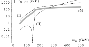
Figure 4: Bosonic contributions to $\Gamma(H\rightarrow\gamma\gamma)$ for $\Lambda=1\,\text{TeV}$ and (I): all $f_{i}=1$ (II): $f_{WW}=1.8$, $f_{BB}=-6.5$, $f_{BW}=-3$, $f_{DW}=5.4$, $f_{WWW}=5.5$, $f_{B}=-4$ and $f_{W}=8$.

In Fig. 4 we have shown two examples of such a dependence, corresponding to different choices of the $f_{i}$’s and with $\Lambda=1\,\text{TeV}$. In the first option, we set all $f_{i}$’s equal to 1. The second (more or less random) choice is designed to demonstrate a possible reduction of the $\Gamma$ in contrast to the otherwise typical enhancement of the SM result.

One could also wonder how much is this process dependent upon the individual constants $f_{i}$. We could expect that the leading contribution comes from the tree level (cf. (21)). It is of course true, but we can imagine a situation where the tree-level contribution is suppressed and the one-loop graphs dominate.

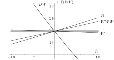
Figure 5: Bosonic contributions to $\Gamma(H\rightarrow\gamma\gamma)$: dependence on a given coefficient $f_{i}$ with all other being set to zero. $m_{H}=120\,\text{GeV}$ and $\Lambda=1\,\text{TeV}$.

From Fig. 5 we can see that apart from $f_{BB}$, $f_{BW}$ and $f_{WW}$ (which are not considered in this plot because of their substantial contribution at the tree level), the $f_{DW}$ can give a rather large contribution.

In the previous discussion we have always set $\Lambda=1\,\text{TeV}$, which is a generic estimate of the new physics scale.

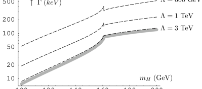
Figure 6: Bosonic contributions to $\Gamma(H\rightarrow\gamma\gamma)$: the dependence on $\Lambda$.

In Fig. 6 we have depicted the dependence of the calculated width $\Gamma$ on the $\Lambda$. As we would expect, effects of the new physics are, roughly speaking, the more important the smaller the scale $\Lambda$ is.

6 Conclusion

Using the effective Lagrangian approach, we have examined the potentially interesting rare decay of the SM-like Higgs boson into two photons. We have considered the “decoupling scenario”, in which the onset of a new physics beyond SM is supposed to be characterized by a mass scale $\Lambda\gg v$. Within such a rather general framework, we have employed a full set of $SU(2)\times U(1)$ invariant dimension-six bosonic effective operators and evaluated, at the one-loop level, the leading $O(1/\Lambda^{2})$ correction to the well-known SM result. Such a calculation seems to be missing in the earlier papers dealing with the $H\rightarrow\gamma\gamma$ process. We have found out that the one-loop contribution involving dimension-six bosonic operators can be very important if there is an accidental suppression of the tree-level effective interaction (i.e. when the combination $f_{BB}-f_{BW}+f_{WW}$ is close to zero). More generally, it is remarkable that the inclusion of dimension-six bosonic operators can change dramatically the bosonic SM contribution; usually it is expected that the effects of new physics beyond SM would enhance the $H\rightarrow\gamma\gamma$ decay rate, but Fig. 4 shows that the effects of the operator (11) could also reduce it significantly.

In our calculation we have ignored completely the effect of fermions. Note that within SM the fermionic contribution to $H\rightarrow\gamma\gamma$ is rather small for the light Higgs (at least at one-loop level) in comparison with bosonic contribution (this follows from straightforward evaluation of (5) and (6)). Within effective Lagrangian approach, the effects of higher-dimensional fermionic operators were studied previously in the paper [11]. Needless to say, a complete realistic calculation would have to take into account an educated guess of the values of the coefficients $f_{i}$ (based on an independent analysis of an appropriate set of other physical processes); in this context see e.g. [16] and references therein. Further work in this direction is in progress.

Appendix A Loop Functions

In evaluating loop integrals we have used the so-called Passarino-Veltman reduction [17], i.e. the reduction of tensor one-loop integrals to the special scalar integrals which can be further expressed by means of some standard analytical functions. In the text we have employed the scalar integrals $B_{0}$, $C_{0}$ and $D_{0}$ defined within dimensional regularization scheme as

$$i\pi^{2}B_{0}(p_{1}^{2},m_{1}^{2},m_{2}^{2})=\int\frac{d^{d}l}{(2\pi\mu)^{d-4}}\frac{1}{[l^{2}-m_{1}^{2}][(l+p_{1})^{2}-m_{2}^{2}]}\,,$$ (25)

$$i\pi^{2}C_{0}(p_{1}^{2},(p_{1}-p_{2})^{2},p_{3}^{2};m_{1}^{2},m_{2}^{2},m_{3}^{2})=\\ \int\frac{d^{d}l}{(2\pi\mu)^{d-4}}\frac{1}{[l^{2}-m_{1}^{2}][(l+p_{1})^{2}-m_{2}^{2}][(l+p_{2})^{2}-m_{3}^{2}]}\,,$$ (26)

$$i\pi^{2}D_{0}(p_{1}^{2},(p_{1}-p_{2})^{2},(p_{2}-p_{3})^{2},p_{3}^{2},p_{2}^{2},(p_{1}-p_{3})^{2};m_{1}^{2},m_{2}^{2},m_{3}^{2},m_{4}^{2})=\\ \int\frac{d^{d}l}{(2\pi\mu)^{d-4}}\frac{1}{[l^{2}-m_{1}^{2}][(l+p_{1})^{2}-m_{2}^{2}][(l+p_{2})^{2}-m_{3}^{2}][(l+p_{3})^{2}-m_{4}^{2}]}\,.$$ (27)

The $C_{0}$ and $D_{0}$ are UV finite while $B_{0}$ is UV divergent for $d=4$. Defining

$$\frac{1}{\tilde{\varepsilon}}=\frac{2}{4-d}-\gamma_{E}+\log 4\pi,$$

we have

$$B_{0}(p^{2},m^{2},m^{2})=\frac{1}{\tilde{\varepsilon}}-\log\frac{m^{2}}{\mu^{2}}+2+{\scriptstyle\sqrt{1-4\frac{m^{2}}{p^{2}}}}\log\frac{{\scriptstyle\sqrt{1-4\frac{m^{2}}{p^{2}}}}-1}{{\scriptstyle\sqrt{1-4\frac{m^{2}}{p^{2}}}}+1}.$$ (28)

One of the three-point functions used in (22) is given by

$$C_{0}(m_{H}^{2},0,0;m_{W}^{2})\equiv C_{0}(m_{H}^{2},0,0;m_{W}^{2},m_{W}^{2},m_{W}^{2})=\\ -\frac{1}{m_{H}^{2}}\Bigl{[}\text{Li}_{2}\Bigl{(}\frac{2}{1-\sqrt{1-4m_{W}^{2}/{m_{H}^{2}}}}\Bigr{)}+\text{Li}_{2}\Bigl{(}\frac{2}{1+\sqrt{1-4m_{W}^{2}/{m_{H}^{2}}}}\Bigr{)}\Bigr{]}\,,$$ (29)

where $\text{Li}_{2}(x)$ is the standard dilogarithm defined through the Spence’s integral:

$$\text{Li}_{2}(x)=-\int_{0}^{x}\frac{\log(1-t)}{t}dt.$$ (30)

Further, let us denote

$$C_{0}(m_{H}^{2},m_{H}^{2},0;m_{W}^{2}) \equiv C_{0}(m_{H}^{2},m_{H}^{2},0;m_{W}^{2},m_{W}^{2},m_{W}^{2})\,,$$

$$D_{0}(m_{H}^{2};m_{W}^{2}) \equiv D_{0}(m_{H}^{2},0,0,0,0,0;m_{W}^{2},m_{W}^{2},m_{W}^{2},m_{W}^{2})\,,$$

$$D_{0}(m_{H}^{2},m_{H}^{2};m_{W}^{2}) \equiv D_{0}(m_{H}^{2},m_{H}^{2},0,0,0,0;m_{W}^{2},m_{W}^{2},m_{W}^{2},m_{W}^{2})\,.$$

A particular linear combination of these quantities appears in the last two lines of eq. (22). The resulting expression comes out to be quite simple, namely

$$2m_{W}^{2}\bigl{(}D_{0}(m_{H}^{2};m_{W}^{2})+2D_{0}(m_{H}^{2},m_{H}^{2};m_{W}^{2})\bigr{)}(m_{H}^{2}-6m_{W}^{2})-C_{0}(\ldots)(m_{H}^{2}+6m_{W}^{2})\\ =\frac{6(m_{H}^{2}-2m_{W}^{2})}{m_{H}\sqrt{4m_{W}^{2}-m_{H}^{2}}}\text{arctan}\Bigl{(}\frac{m_{H}}{\sqrt{4m_{W}^{2}-m_{H}^{2}}}\Bigr{)}\,.$$ (31)

Note finally that the proper analytic continuation of the above functions is obtained by means of the prescription $m^{2}\rightarrow m^{2}-i\varepsilon$ wherever it is necessary.

References

- [1] R. Barate et al. [ALEPH Collaboration], Phys. Lett. B 565 (2003) 61 [arXiv:hep-ex/0306033].
- [2] P. Sikivie, L. Susskind, M. B. Voloshin and V. I. Zakharov, Nucl. Phys. B 173 (1980) 189.
- [3] L. J. Hall, Beyond the standard model, ICHEP 2000, Osaka, Japan, 27 Jul - 2 Aug 2000.
- [4] J. Wudka, Int. J. Mod. Phys. A 9 (1994) 2301 [arXiv:hep-ph/9406205].
- [5] J. Novotný and M. Stöhr, Czech. J. Phys. 49 (1999) 1471 [arXiv:hep-ph/9904401].
- [6] W. Buchmüller and D. Wyler, Nucl. Phys. B 268 (1986) 621.
- [7] K. Hagiwara, S. Ishihara, R. Szalapski and D. Zeppenfeld, Phys. Rev. D 48 (1993) 2182.
- [8] K. Cranmer, B. Mellado, W. Quayle and S. L. Wu, arXiv:hep-ph/0401088.
- [9] J. R. Ellis, M. K. Gaillard and D. V. Nanopoulos, Nucl. Phys. B 106 (1976) 292; M. A. Shifman, A. I. Vainshtein, M. B. Voloshin and V. I. Zakharov, Sov. J. Nucl. Phys. 30 (1979) 711 [Yad. Fiz. 30 (1979) 1368].
- [10] H. König, Phys. Rev. D 45 (1992) 1575.
- [11] J. M. Hernandez, M. A. Perez and J. J. Toscano, Phys. Rev. D 51 (1995) 2044; M. A. Perez, J. J. Toscano and J. Wudka, Phys. Rev. D 52 (1995) 494 [arXiv:hep-ph/9506457].
- [12] A. T. Banin, I. F. Ginzburg and I. P. Ivanov, Phys. Rev. D 59 (1999) 115001 [arXiv:hep-ph/9806515].
- [13] J. Hořejší: Fundamentals of Electroweak Theory (Karolinum Press, Prague 2002).
- [14] D. Y. Bardin and G. Passarino: The Standard Model In The Making: Precision Study Of The Electroweak Interactions (Clarendon Press, Oxford 1999).
- [15] H. Arason, D. J. Castano, B. Keszthelyi, S. Mikaelian, E. J. Piard, P. Ramond and B. D. Wright, Phys. Rev. D 46 (1992) 3945.
- [16] B. Zhang, Y. P. Kuang, H. J. He and C. P. Yuan, Phys. Rev. D 67 (2003) 114024 [arXiv:hep-ph/0303048].
- [17] G. Passarino and M. J. Veltman, Nucl. Phys. B 160 (1979) 151.