Complete description of polarization effects in emission of
a photon by an electron in the field of a strong laser wave

Abstract

We consider emission of a photon by an electron in the field of a strong laser wave. Polarization effects in this process are important for a number of physical problems. The probability of this process for circularly or linearly polarized laser photons and for arbitrary polarization of all other particles is calculated. We obtain the complete set of functions which describe such a probability in a compact invariant form. Besides this, we discuss in some detail the polarization effects in the kinematics relevant to the problem of $e\to\gamma$ conversion at $\gamma\gamma$ and $\gamma e$ colliders.

1 Introduction

The Compton scattering

$$e(p)+\gamma(k)\to e(p^{\prime})+\gamma(k^{\prime})$$ (1)

is one of the first processes calculated in quantum electrodynamics at the end of 1920’s. The analysis of polarization effects in this reaction is now included in text-books (see, for example, BLP §87). Nevertheless, the complete description of cross sections with polarization of both initial and final particles has been considered in detail only recently (see Grozin ; GKPS83 ; KPS98 and literature therein). One interesting application is the collision of an ultra-relativistic electron with a beam of polarized laser photons. In this case the Compton effect is the basic process for obtaining of high-energy photons for contemporary experiments in nuclear physics (photo-nuclear reactions with polarized photons) and for future $\gamma\gamma$ and $\gamma e$ colliders GKST83 . The importance of the particle polarization is clearly seen from the fact that in comparison with the unpolarized case the number of final photons with maximum energy is nearly doubled when the helicities of the initial electron and photon are opposite GKPS83 .

With the growth of the laser field intensity, an electron starts to interact coherently with $n$ laser photons,

$$e(q)+n\,\gamma_{L}(k)\to e(q^{\prime})+\gamma(k^{\prime})\,,$$ (2)

thus the Compton scattering becomes non-linear. Such a process with absorption of $n=1,\,2,\,3,\,4$ linearly polarized laser photons was observed in the recent experiment at SLAC SLAC . The polarization properties of the process (2) are important for a number of problems, for example, for laser beam cooling Telnov and, especially, for future $\gamma\gamma$ and $\gamma e$ colliders (see GKPnQED ; GKLT2001 and the literature therein) . In the latter case the non-linear Compton scattering must be taken into account in simulations of the processes in the conversion region. For comprehensive simulation, including processes of multiple electron scattering, one has to know not only the differential cross section of the non-linear Compton scattering with a given number of the absorbed laser photons $n$, but energy, angles and polarization of final photons and electrons as well. The method of calculation for such cross sections was developed by Nikishov and Ritus NR-review . It is based on the exact solution of the Dirac equation in the field of the external electromagnetic plane wave. Some particular polarization properties of this process were considered in NR-review –BPM and have already been included in the existing simulation codes Yokoya ; TCode . Another approach was used in BKMS , where the total cross section and the spectrum for the non-linear Compton scattering, summed over numbers of the absorbed laser photons $n$ and over spin states of the final particles, had been obtained.

In the present paper we give the complete description of the non-linear Compton scattering for the case of circularly or linearly polarized laser photons and arbitrary polarization of all other particles. We follow the method of Nikishov and Ritus in the form presented in BLP §101. In the next section we describe in detail the kinematics of the process (2). The effective differential cross section is obtained in Sect. 3 in the compact invariant form, including the polarization of all particles. In Sect. 4 we consider the process (2) in the reference frame relevant for $\gamma\gamma$ and $\gamma e$ colliders. The limiting cases are discussed in Sect. 5. In Sect. 6 we present some numerical results obtained for the range of parameters close to those in the existing projects of the $\gamma\gamma$ and $\gamma e$ colliders. In the last section we summarize our results and compare them with those known in the literature. In Appendix A we show that our results coincide in the limit of weak laser field with those for the linear Compton scattering.

2 Kinematics

2.1 Parameter of non-linearity

Let us consider the interaction of an electron with a monochromatic plane wave described by the 4-potential $A_{\mu}(x)$. The corresponding electric and magnetic fields are ${\bf E}$ and ${\bf B}$, a frequency is $\omega$, and let $F$ be the root-mean-squared field strength,

$$F^{2}=\langle{\bf B}^{2}\rangle=\langle{\bf E}^{2}\rangle\,.$$

The invariant parameter describing the intensity of the laser field (the parameter of non-linearity) is defined via the mean value of the squared 4-potential:

$$\xi={e\over mc^{2}}\sqrt{-\langle A_{\mu}(x)A^{\mu}(x)\rangle}\,,$$ (3)

where $e$ and $m$ are the electron charge and the mass, and $c$ is the velocity of light. We use this definition of $\xi$ both for the circularly and linearly polarized laser photons.

The origin of this parameter can be explained as follows. The electron oscillates in the transverse direction under the influence of a force $\sim eF$ and for the time $\sim 1/\omega$ acquires the transverse momentum $\sim p_{\perp}=eF/\omega$, thus for the longitudinal motion the effective electron mass is $m_{*}=\sqrt{m^{2}+(p_{\perp}/c)^{2}}$. The ratio of the momentum $p_{\perp}$ to $mc$ is the natural dimensionless parameter

$$\xi={eF\over m\,c\,\omega}\,.$$ (4)

This parameter can be expressed also via the density $n_{\rm L}$ of photons in the laser wave:

$$\xi^{2}=\left({eF\over m\omega c}\right)^{2}={4\pi\alpha\hbar^{2}\over m^{2}c\,\omega}\,n_{\rm L}\,,$$ (5)

where $\hbar$ is the Plank constant and $\alpha=e^{2}/(\hbar c)\approx 1/137$.

2.2 Invariant variables

From the classical point of view, the oscillated electron emits harmonics with frequencies $n\,\omega$, where $n=1,\;2,\;\dots$ Their intensities at small $\xi^{2}$ are proportional to $({\bf E}^{2})^{n}\propto\xi^{2n}$, the polarization properties of these harmonics depend on the polarizations of the laser wave and the initial electron. From the quantum point of view, this radiation can be described as the non-linear Compton scattering with absorption of $n$ laser photons. When describing such a scattering, one has to take into account that in a laser wave the 4-momenta $p$ and $p^{\prime}$ of the free initial and final electrons are replaced by the 4-quasi-momenta $q$ and $q^{\prime}$ (similar to the description of a particle motion in a periodic potential field in non-relativistic quantum mechanics),

$$q = p+\xi^{2}{m^{2}c^{2}\over 2pk}\,k\,,\;\;q^{\prime}=p^{\prime}+\xi^{2}{m^{2}c^{2}\over 2p^{\prime}k}\,k\,,$$ (6)

$$q^{2} = (q^{\prime})^{2}=(1+\xi^{2})\,m^{2}c^{2}\equiv m_{*}^{2}c^{2}\,.$$

In particular, the energy of the free incident electron $E$ is replaced by the quasi-energy

$$cq_{0}=E+\xi^{2}{m^{2}c^{2}\over 2pk}\,\hbar\omega\,.$$ (7)

As a result, we deal with the reaction (2) for which the conservation law reads

$$q+n\,k=q^{\prime}+k^{\prime}\,.$$ (8)

From this it follows that all the kinematic relations which occur for the linear Compton scattering will apply to the process considered here if the electron momenta $p$ and $p^{\prime}$ are replaced by the quasi-momenta $q$ and $q^{\prime}$ and the incident photon momentum $k$ by the 4-vector $nk$. Since $qk=pk$, it is convenient to use the same invariant variables as for the linear Compton scattering (compare GKPS83 ):

$$x={2pk\over m^{2}c^{2}}\,,\;\;\;y\;={kk^{\prime}\over pk}\,.$$ (9)

Moreover, many kinematic relations can be obtained from that for the linear Compton scattering by the replacement $\omega\to n\,\omega$, $m\to m_{*}$. In particular, we introduce the auxiliary combinations

$$s_{n}=2\sqrt{r_{n}(1-r_{n})},\;\;c_{n}=1-2r_{n}\,,$$ (10)

where

$$r_{n}={y\,(1+\xi^{2})\over(1-y)\,nx}\,.$$ (11)

It is useful to note that these invariants have a simple notion, namely

$$s_{n}=\sin{\tilde{\theta}},\;\;c_{n}=\cos{\tilde{\theta}}\,,\;\;r_{n}=\sin^{2}(\tilde{\theta}/2)\,,$$ (12)

where $\tilde{\theta}$ is the photon scattering angle in the frame of reference where the initial electron is at rest on average (${\bf q}=0,\,q_{0}=m_{*}c$). Therefore,

$$0\leq s_{n},\;r_{n}\leq 1\,;\;\;-1\leq c_{n}\leq 1\,.$$ (13)

The maximum value of the variable $y$ for the reaction (2) is

$$y\leq\;y_{n}\;={nx\over nx+1+\xi^{2}}\,.$$ (14)

The value of $y_{n}$ is close to $1$ for large $n$, but for a given $n$ it decreases with the growth of the non-linearity parameter $\xi^{2}$. With this notation one can rewrite $s_{n}$ in the form

$$s_{n}={2\over y_{n}(1-y)}\,\sqrt{y(y_{n}-y)(1-y_{n})}\,,$$ (15)

from which it follows that

$$s_{n}\to 0\;\;\mbox{ at }\;\;y\to y_{n}\;\;\mbox{or at}\;\;y\to 0\,.$$ (16)

The usual notion of the cross section is not applicable for the reaction (2) and usually its description is given in terms of the probability of the process per second $\dot{W}^{(n)}$. However, for the procedure of simulation in the conversion region as well as for the simple comparison with the linear case, it is useful to introduce the “effective cross section” given by the definition

$$d\sigma^{(n)}={d\dot{W}^{(n)}\over j}\,,$$ (17)

where

$$j={(q\,k)c^{2}\over q_{0}\,\hbar\omega}\,n_{\rm L}={m^{2}c^{4}\,x\over 2q_{0}\hbar\omega}\,n_{\rm L}$$

is the flux density of colliding particles. Contrary to the usual cross section, this effective cross section does depend on the laser beam intensity, i.e. on the parameter $\xi^{2}$. The total effective cross section is defined as the sum over harmonics, corresponding to the reaction (2) with a given number $n$ of the absorbed laser photons:

$$d\sigma=\sum\limits_{n}d\sigma^{(n)}\,.$$ (18)

2.3 Invariant polarization parameters

The invariant description of the polarization properties of both the initial and the final photons can be performed in the standard way (see BLP , §87). We define a pair of unit 4-vectors

$$e^{(1)}={N\over\sqrt{-N^{2}}}\,,\;\;\;e^{(2)}={P\over\sqrt{-P^{2}}}\,,$$ (19)

where

$$N^{\mu} = \varepsilon^{\mu\alpha\beta\gamma}P_{\alpha}(k^{\prime}-n\,k)_{\beta}K_{\gamma}\,,$$

$$P_{\alpha} = (q+q^{\prime})_{\alpha}-{(q+q^{\prime})K\over K^{2}}\,K_{\alpha}\,,\;\;\;K_{\alpha}=n\,k_{\alpha}+k^{\prime}_{\alpha}\,,$$

$$\sqrt{-N^{2}} = m^{3}xy\,{n\,s_{n}\over r_{n}}\sqrt{1+\xi^{2}}\,,\;\;\;\sqrt{-P^{2}}=m\,{s_{n}\over r_{n}}\sqrt{1+\xi^{2}}\,.$$

The 4-vectors $e^{(1)}$ and $e^{(2)}$ are orthogonal to each other and to the 4-vectors $k$ and $k^{\prime}$,

$$e^{(i)}e^{(j)}=-\delta_{ij},\;\;e^{(i)}k=e^{(i)}k^{\prime}=0;\;\;i,\,j=1,\,2\,.$$

Therefore, they are fixed with respect to the scattering plane of the process.

Let $\xi_{j}$ be the Stokes parameters for the initial photon which are defined with respect to 4-vectors $e^{(1)}$ and $e^{(2)}$. As for the polarization of the final photon, it is necessary to distinguish the polarization $\xi_{j}^{(f)}$ of the final photon as resulting from the scattering process itself from the detected polarization $\xi^{\prime}_{j}$ which enters the effective cross section and which essentially represents the properties of the detector as selecting one or other polarization of the final photon (for detail see BLP , §65). Both these Stokes parameters, $\xi_{j}^{(f)}$ and $\xi^{\prime}_{j}$, are also defined with respect to the 4-vectors $e^{(1)}$ and $e^{(2)}$.

Let $\zeta$ be the polarization vector of the initial electrons. As with the final photon, it is necessary to distinguish the polarization $\zeta$^(f) of the final electron as such from the polarization $\zeta$^′ that is selected by the detector. The vectors $\zeta$ and $\zeta$^′ enter the effective cross section. They also determine the electron-spin 4-vectors

$$a = \left({\mbox{\boldmath$\zeta$}{\bf p}\over m}\,,\,\mbox{\boldmath$\zeta$}+{\bf p}{\mbox{\boldmath$\zeta$}{\bf p}\over m(E+m)}\right)\,,$$

$$a^{\prime} = \left({\mbox{\boldmath$\zeta$}^{\prime}{\bf p}^{\prime}\over m}\,,\,\mbox{\boldmath$\zeta$}^{\prime}+{\bf p}^{\prime}{\mbox{\boldmath$\zeta$}^{\prime}{\bf p}^{\prime}\over m(E^{\prime}+m)}\right)$$ (20)

and the mean helicity of the initial and final electrons

$$\lambda_{e}={\mbox{\boldmath$\zeta$}{\bf p}\over 2|{\bf p}|}\,,\;\;\;\;\lambda^{\prime}_{e}={\mbox{\boldmath$\zeta$}^{\prime}{\bf p}^{\prime}\over 2|{\bf p}^{\prime}|}\,.$$ (21)

Now we have to define invariants which describe the polarization properties of the initial and the final electrons. For the electrons it is a more complicated task than it is for the photons. For the linear Compton scattering, the relatively simple description was obtained in  Grozin using invariants which have a simple meaning in the center-of-mass system. However, this frame of reference is not convenient for the description of the non-linear Compton scattering, since it has actually to vary with the change of the number of the absorbed laser photons $n$.

Since $ap=a^{\prime}p^{\prime}=0$, we can decompose the electron polarization 4-vectors over three convenient unit 4-vectors $e_{j}$ and $e_{j}^{\prime}$, $j=1,\,2,\,3$, projections on which determine polarization properties of the electrons. Our choice is based on the experience obtained in KPS98 and BPM . We exploit two ideas. First of all, the 4-vector $e^{(1)}$ is orthogonal to the 4-vectors $k,\;k^{\prime},\;p$ and $p^{\prime}$, therefore, the invariants $\zeta_{1}=-ae^{(1)}$ and $\zeta^{\prime}_{1}=-a^{\prime}e^{(1)}$ are the transverse polarizations of the initial and the final electrons perpendicular to the scattering plane. Further, it is not difficult to check that the invariant $ak/(mx)$ is the mean helicity of the initial electron in the frame of reference, in which the electron momentum ${\bf p}$ is anti-parallel to the initial photon momentum ${\bf k}$. Analogously, the invariant $a^{\prime}k/[(mx(1-y)]$ is the mean helicity of the final electron in the frame of reference, in which the momentum of the final electron ${\bf p}^{\prime}$ is anti-parallel to the initial photon momentum ${\bf k}$. It is important that this interpretation is valid for any number of absorbed laser photons. Furthermore, we will show that for the practically important case, relevant for the $e\to\gamma$ conversion, these frames of reference almost coincide.

As a result, we define the two sets of units 4-vectors

$$e_{1} = e^{(1)}\,,\;\;\;e_{2}=-e^{(2)}-{\sqrt{-P^{2}}\over m^{2}x}k\,,$$

$$e_{3} = {1\over m}\left(p-{2\over x}k\right);$$ (22)

$$e^{\prime}_{1} = e^{(1)}\,,\;\;\;e^{\prime}_{2}=-e^{(2)}-{\sqrt{-P^{2}}\over m^{2}x(1-y)}k\,,$$

$$e^{\prime}_{3} = {1\over m}\left(p^{\prime}-{2\over x(1-y)}k\right).$$

These vectors satisfy the conditions

$$e_{i}e_{j}=-\delta_{ij}\;,\;\;\;e_{j}p=0\;;\;\;\;e^{\prime}_{i}e^{\prime}_{j}=-\delta_{ij}\;,\;\;\;e^{\prime}_{j}p^{\prime}=0\,.$$ (23)

It allows us to represent the 4-vectors $a$ and $a^{\prime}$ in the following covariant form:

$$a=\sum_{j=1}^{3}\zeta_{j}e_{j}\,,\;\;\;a^{\prime}=\sum_{j=1}^{3}\zeta^{\prime}_{j}e^{\prime}_{j}\,,$$ (24)

where

$$\zeta_{j}=-ae_{j}\,,\;\;\;\zeta^{\prime}_{j}=-a^{\prime}e^{\prime}_{j}\,.$$ (25)

The invariants $\zeta_{j}$ and $\zeta^{\prime}_{j}$ describe completely the polarization properties of the initial electron and the detected polarization properties of the final electron, respectively. To clarify the meaning of invariants $\zeta_{j}$, it is useful to note that

$$\zeta_{j}={\mbox{\boldmath$\zeta$}}{\bf n}_{j}\,,$$ (26)

where the corresponding 3-vectors are

$${\bf n}_{j}={\bf e}_{j}-{{\bf p}\over E+m}\;e_{j0}$$ (27)

with $e_{j0}$ being a time component of the 4-vector $e_{j}$ defined in (22). Using the properties (23) of the 4-vectors $e_{j}$, one can check that

$${\bf n}_{i}\;{\bf n}_{j}=\delta_{ij}\,.$$ (28)

As a result, the polarization vector $\zeta$ has the form

$$\mbox{\boldmath$\zeta$}=\sum^{3}_{j=1}\zeta_{j}\;{\bf n}_{j}\,.$$ (29)

Analogously, for the final electron the invariants $\zeta^{\prime}_{j}$ can be presented as

$$\zeta^{\prime}_{j}={\mbox{\boldmath$\zeta$}}^{\prime}{\bf n}^{\prime}_{j},\;\;\;{\bf n}^{\prime}_{j}={\bf e}^{\prime}_{j}-{{\bf p}^{\prime}\over E^{\prime}+m}\;e^{\prime}_{j0},\;\;\;{\bf n}^{\prime}_{i}\;{\bf n}^{\prime}_{j}=\delta_{ij}\,,$$ (30)

such that

$$\mbox{\boldmath$\zeta$}^{\prime}=\sum^{3}_{j=1}\zeta^{\prime}_{j}\;{\bf n}^{\prime}_{j}\,.$$ (31)

In what follows, we will often consider the non-linear Compton scattering in the frame of reference in which an electron performs a head-on collision with laser photons, i.e. in which ${\bf p}\,\parallel\,(-{\bf k})$. We call this the “collider system”. In this frame of reference we choose the $z$-axis along the initial electron momentum ${\bf p}$. Azimuthal angles $\varphi,\;\beta$ and $\beta^{\prime}$ of vectors ${\bf k}^{\prime},\;\mbox{\boldmath$\zeta$}$ and $\mbox{\boldmath$\zeta$}^{\prime}$ are defined with respect to one fixed $x$-axis.

3 Cross section in the invariant form

3.1 General relations

The effective differential cross section can be presented in the following invariant form:

$$d\sigma(\mbox{\boldmath$\zeta$},\,\mbox{\boldmath$\xi$},\,\mbox{\boldmath$\zeta$}^{\prime},\,\mbox{\boldmath$\xi$}^{\prime})={r_{e}^{2}\over 4x}\;\sum_{n}F^{(n)}\;d\Gamma_{n}\,,$$ (32)

$$d\Gamma_{n}=\delta(q+n\,k-q^{\prime}-k^{\prime})\;{d^{3}k^{\prime}\over\omega^{\prime}}{d^{3}q^{\prime}\over q_{0}^{\prime}}\,,$$

where $r_{e}=\alpha/m$ is the classical electron radius, and

$$F^{(n)} = F_{0}^{(n)}+\sum^{3}_{j=1}\left(F_{j}^{(n)}\xi^{\prime}_{j}\;+\;G_{j}^{(n)}\zeta^{\prime}_{j}\right)$$ (33)

$$+ \sum^{3}_{i,j=1}H_{ij}^{(n)}\,\zeta^{\prime}_{i}\,\xi^{\prime}_{j}\,.$$

Here the function $F_{0}^{(n)}$ describes the total cross section for a given harmonic $n$, summed over spin states of the final particles:

$$\sigma^{(n)}(\mbox{\boldmath$\zeta$},\,\mbox{\boldmath$\xi$})={r_{e}^{2}\over x}\;\int F_{0}^{(n)}\,d\Gamma_{n}\,.$$ (34)

The terms $F_{j}^{(n)}\xi^{\prime}_{j}$ and $G_{j}^{(n)}\zeta^{\prime}_{j}$ in (33) describe the polarization of the final photons and the final electrons, respectively. The last terms $H_{ij}^{(n)}\zeta^{\prime}_{i}\,\xi^{\prime}_{j}$ stand for the correlation of the final particles’ polarizations.

From (32), (33) one can deduce the polarization of the final photon $\xi_{j}^{(f)}$ and electron $\zeta^{(f)}_{j}$ resulting from the scattering process itself. According to the usual rules (see BLP , §65), we obtain the following expression for the Stokes parameters of the final photon (summed over polarization states of the final electron):

$$\xi_{j}^{(f)} = {F_{j}\over F_{0}}\,,\;\;F_{0}=\sum_{n}F_{0}^{(n)}\,,\;\;F_{j}=\sum_{n}F_{j}^{(n)}\,;$$

$$j = 1,\,2,\,3\,.$$ (35)

The polarization of the final electron (summed over polarization states of the final photon) is given by invariants

$$\zeta_{j}^{(f)}={G_{j}\over F_{0}}\,,\;\;G_{j}=\sum_{n}G_{j}^{(n)}\,,$$ (36)

therefore, its polarization vector is

$$\mbox{ \boldmath$\zeta$}^{(f)}=\sum_{j=1}^{3}\,{G_{j}\over F_{0}}\,{\bf n}_{j}^{\prime}\,.$$ (37)

In the similar way, the polarization properties for a given harmonic $n$ are described by

$$\xi_{j}^{(n)(f)}={F_{j}^{(n)}\over F_{0}^{(n)}}\,,\;\;\zeta_{j}^{(n)(f)}={G_{j}^{(n)}\over F_{0}^{(n)}}\,.$$ (38)

3.2 The results for the circularly polarized laser photons

In this subsection we consider the case of 100% circularly polarized laser beam. The electromagnetic laser field is described by the 4-potential

$$A_{\mu}(x)={m\over e}\,\xi\;\left[e_{\mu}^{(1)}\,\cos{(kx)}+P_{c}\,e_{\mu}^{(2)}\,\sin{(kx)}\right]\,,$$ (39)

where the unit vectors $e_{\mu}^{(1,2)}$ are given in (19) and $P_{c}$ is the degree of the circular polarization of the laser wave or the initial photon helicity. Therefore, the Stokes parameters of the laser photon are

$$\xi_{1}=\xi_{3}=0,\;\;\xi_{2}=P_{c}=\pm 1\,.$$ (40)

We have calculated the coefficients $F_{j}^{(n)},\,G_{j}^{(n)}$ and $H_{ij}^{(n)}$ using the standard technique presented in BLP , §101. The necessary traces have been calculated using the package MATHEMATICA. In the considered case of the 100 % circularly polarized ($P_{c}=\pm 1$) laser beam, almost all dependence on the non-linearity parameter $\xi^{2}$ accumulates in three functions:

$$f_{n} \equiv f_{n}(z_{n})=J_{n-1}^{2}(z_{n})+J_{n+1}^{2}(z_{n})-2J_{n}^{2}(z_{n})\,,$$

$$g_{n} \equiv g_{n}(z_{n})=\frac{4n^{2}J_{n}^{2}(z_{n})}{z_{n}^{2}}\,,$$ (41)

$$h_{n} \equiv h_{n}(z_{n})=J_{n-1}^{2}(z_{n})-J_{n+1}^{2}(z_{n})\,,$$

where $J_{n}(z)$ is the Bessel function. The functions (41) depend on $x$, $y$ and $\xi$ via the single argument

$$z_{n}={\xi\over\sqrt{1+\xi^{2}}}\;n\,s_{n}\,.$$ (42)

For the small value of this argument one has

$$f_{n}=g_{n}=h_{n}=\frac{(z_{n}/2)^{2(n-1)}}{[(n-1)!]^{2}}\;\;\mbox{ at}\;\;z_{n}\to 0\,,$$ (43)

in particular,

$$f_{1}=g_{1}=h_{1}=1\;\;\mbox{ at}\;\;z_{1}=0\,.$$ (44)

It is useful to note that this argument is small for small $\xi^{2}$, as well as for small or for large values of $y$:

$$z_{n} \to 0\;\;\mbox{either at}\;\;\xi^{2}\to 0\,,$$ (45)

$$\mbox{ or at }\;\;y\to 0\,,\;\;\mbox{ or at }\;\;y\to y_{n}\,.$$

The results of our calculations are the following. The function $F_{0}^{(n)}$, related to the total cross section (34), reads

$$F_{0}^{(n)} = \left({1\over 1-y}+1-y\right)\,f_{n}-{s_{n}^{2}\over 1+\xi^{2}}\,g_{n}$$ (46)

$$- \left[{ys_{n}\over\sqrt{1+\xi^{2}}}\,\zeta_{2}-{y(2-y)\over 1-y}\,c_{n}\,\zeta_{3}\right]\,h_{n}\,P_{c}\,.$$

The polarization of the final photons $\xi_{j}^{(f)}$ is given by Eq. (35) where

$$F_{1}^{(n)} = {y\over 1-y}{s_{n}\over\sqrt{1+\xi^{2}}}\,h_{n}P_{c}\,\zeta_{1}\,,$$ (47)

$$F_{2}^{(n)} = \left({1\over 1-y}+1-y\right)\,c_{n}h_{n}P_{c}-{ys_{n}c_{n}\over\sqrt{1+\xi^{2}}}\,g_{n}\,\zeta_{2}$$

$$+ y\left({2-y\over 1-y}\,f_{n}-{s^{2}_{n}\over 1+\xi^{2}}\,g_{n}\right)\zeta_{3}\,,$$

$$F_{3}^{(n)} = 2(f_{n}-g_{n})+s^{2}_{n}(1+\Delta)\,g_{n}$$

$$- {y\over 1-y}{s_{n}\over\sqrt{1+\xi^{2}}}\,h_{n}P_{c}\,\zeta_{2}\,;$$

here and below we use the notation

$$\Delta={\xi^{2}\over 1+\xi^{2}}\,.$$ (48)

The polarization of the final electrons $\zeta_{j}^{(f)}$ is given by (36), (37) with

$$G_{1}^{(n)} = \,G^{(n)}_{\perp}\,\zeta_{1},$$ (49)

$$G_{2}^{(n)} = \,G^{(n)}_{\perp}\,\,\zeta_{2}-\frac{y{s}_{n}}{(1-y)\sqrt{1+\xi^{2}}}\,\left(c_{n}\,g_{n}\,\zeta_{3}+h_{n}\,P_{c}\right)\,,$$

$$G_{3}^{(n)} = \,G^{(n)}_{\parallel}+\,\frac{y{s}_{n}{c}_{n}}{\sqrt{1+\xi^{2}}}\,g_{n}\,\zeta_{2},$$

where we introduced the notation

$$G_{\perp}^{(n)} = 2f_{n}-\frac{{s}_{n}^{2}}{1+\xi^{2}}\,g_{n}\,,$$ (50)

$$G^{(n)}_{\parallel} = \left[\left(\frac{1}{1-y}+1-y\right)f_{n}\right.$$

$$- \left.\left(1+\frac{y^{2}}{1-y}\right)\frac{{s_{n}^{2}}}{1+\xi^{2}}g_{n}\right]\zeta_{3}+\frac{y(2-y){c}_{n}}{1-y}\,h_{n}P_{c}\,.$$

Finally, the correlations of the final particles’ polarizations are

$$H_{11}^{(n)} = \frac{ys_{n}}{\sqrt{1+\xi^{2}}}h_{n}P_{c}+\frac{y}{1-y}\left[(2-y)(f_{n}-g_{n})\right.$$

$$+ \left.(1-y+\Delta)s_{n}^{2}g_{n}\right]\zeta_{2}-\frac{yc_{n}s_{n}}{\sqrt{1+\xi^{2}}}g_{n}\zeta_{3},$$

$$H_{21}^{(n)} = -\frac{y}{1-y}\left\{(2-y)(f_{n}-g_{n})\right.$$

$$+ \left.\left[1+(1-y)\Delta\right]s_{n}^{2}g_{n}\right\}\zeta_{1}\,,$$

$$H_{31}^{(n)} = \frac{yc_{n}s_{n}}{(1-y)\sqrt{1+\xi^{2}}}g_{n}\zeta_{1}\,,\ \ \ H_{12}^{(n)}=2c_{n}h_{n}P_{c}\,\zeta_{1}\,,$$

$$H_{22}^{(n)} = -\frac{yc_{n}s_{n}}{(1-y)\sqrt{1+\xi^{2}}}\,g_{n}+2c_{n}h_{n}P_{c}\,\zeta_{2}$$ (52)

$$- \frac{ys_{n}}{(1-y)\sqrt{1+\xi^{2}}}\,h_{n}P_{c}\,\zeta_{3}\,,$$

$$H_{32}^{(n)} = \frac{y}{1-y}\left[(2-y)f_{n}-\frac{s_{n}^{2}}{1+\xi^{2}}g_{n}\right]+\frac{ys_{n}}{\sqrt{1+\xi^{2}}}\,h_{n}P_{c}\,\zeta_{2}$$

$$+ \frac{2-2y+y^{2}}{1-y}\,c_{n}h_{n}P_{c}\,\zeta_{3}\,,$$

$$H_{13}^{(n)} = \left[\frac{2-2y+y^{2}}{1-y}(f_{n}-g_{n})\right.$$

$$+ \left.\left(1+\frac{1-y+y^{2}}{1-y}\Delta\right)s_{n}^{2}\,g_{n}\right]\,\zeta_{1}\,,$$

$$H_{23}^{(n)} = -\frac{ys_{n}}{\sqrt{1+\xi^{2}}}\,h_{n}P_{c}+\left[\frac{2-2y+y^{2}}{1-y}(f_{n}-g_{n})\right.$$

$$+ \left.\left(\frac{1-y+y^{2}}{1-y}+\Delta\right)\,s_{n}^{2}\,g_{n}\right]\,\zeta_{2}$$

$$+ \frac{yc_{n}s_{n}}{\sqrt{1+\xi^{2}}}\,g_{n}\,\zeta_{3}\,,$$

$$H_{33}^{(n)} = -\frac{yc_{n}s_{n}}{(1-y)\sqrt{1+\xi^{2}}}\,g_{n}\,\zeta_{2}$$

$$+ \left[2(f_{n}-g_{n})+(1+\Delta)\,s_{n}^{2}\,g_{n}\right]\,\zeta_{3}\,.$$

3.3 The results for the linearly polarized laser photons

Here we consider the case of 100% linearly polarized laser beam. The electromagnetic laser field is described by the 4-potential

$$A^{\mu}(x) = A^{\mu}\,\cos{(kx)}\,,\;\;A^{\mu}={\sqrt{2}\,m\over e}\,\xi\;e_{\rm L}^{\mu}\,,$$

$$e_{\rm L}e_{\rm L} = -1\,,$$ (53)

where $e^{\mu}_{\rm L}$ is the unit 4-vector describing the polarization of the laser photons, which can be expressed in the covariant form via the unit 4-vectors $e^{(1,2)}$ given in (19) as follows:

$$e_{\rm L}=e^{(1)}\,\sin{\varphi}-e^{(2)}\,\cos{\varphi}\,.$$ (54)

The invariants

$$\sin{\varphi}=-e_{\rm L}\,e^{(1)}\,,\;\;\;\cos{\varphi}=e_{\rm L}\,e^{(2)}$$ (55)

have a simple notion in the collider system. For the problem discussed it is convenient to choose the $x$-axis of this frame of reference along the direction of the laser linear polarization, i.e. along the vector ${\bf e}_{{\rm L}\perp}$. With such a choice, the quantity $\varphi$ is the azimuthal angle of the final photon in the collider system (analogously, the azimuthal angles $\beta$ and $\beta^{\prime}$ of the electron polarizations $\zeta$ and $\mbox{\boldmath$\zeta$}^{\prime}$ are also defined with respect to this $x$-axis).

The Stokes parameters $\xi_{i}$ are defined with respect to the $x^{\prime}y^{\prime}z^{\prime}$-axes which are fixed to the scattering plane. The $x^{\prime}$-axis is perpendicular to the scattering plane:

$$x^{\prime}\;\parallel\;{\bf k}\times{\bf k}^{\prime};$$ (56)

the $y^{\prime}$-axis is in that plane

$$y^{\prime}\;\parallel\;{\bf k}\times({\bf k}\times{\bf k}^{\prime})=-\omega^{2}{\bf k}^{\prime}_{\perp}\,.$$ (57)

The azimuthal angle of the linear polarization of the laser photon in the collider system equals zero with respect to the $xyz$-axes, and it is $\varphi+(3\pi/2)$ with respect to the $x^{\prime}y^{\prime}z^{\prime}$-axes. Therefore, in the considered case of the 100 % linearly polarized laser beam one has

$$\xi_{1}=-\sin{2\varphi},\;\;\;\xi_{2}=0,\;\;\;\xi_{3}=-\cos{2\varphi}\,.$$ (58)

When calculating the effective cross section (32), we found that almost all dependence on the non-linearity parameter $\xi^{2}$ accumulates in three functions:

$$\tilde{f}_{n} = 4\left[A_{1}(n,\,a,\,b)\right]^{2}-4A_{0}(n,\,a,\,b)A_{2}(n,\,a,\,b)\,,$$

$$\tilde{g}_{n} = {4n^{2}\over z_{n}^{2}}\,\left[A_{0}(n,\,a,\,b)\right]^{2}\,,$$ (59)

$$\tilde{h}_{n} = {4n\over a}\,A_{0}(n,\,a,\,b)\,A_{1}(n,\,a,\,b)\,,$$

where the functions $A_{k}(n,\,a,\,b)$ were introduced in NR-review as follows

$$A_{k}(n,\,a,\,b)$$ (60)

$$=\int\limits_{-\pi}^{\pi}\,\cos^{k}{\psi}\,\exp{\left[\,{\rm i}\left(n\psi-a\sin{\psi}+b\sin{2\psi}\right)\right]}\,{d\psi\over 2\pi}\,.$$

The arguments of these functions are

$$a=e\,\left({Ap\over kp}-{Ap{{}^{\prime}}\over kp^{\prime}}\right)\,,\;\;b={1\over 8}\,e^{2}A^{2}\,\left({1\over kp}-{1\over kp^{\prime}}\right)$$ (61)

or, expressed in terms of the non-linearity parameter, they are

$$a=\sqrt{2}\,\xi\,m\,\left({e_{\rm L}p\over kp}-{e_{\rm L}p^{\prime}\over kp^{\prime}}\right)\,,\;\;b={y\over 2(1-y)x}\,\xi^{2}\,.$$ (62)

In the collider system one has

$$a=-z_{n}\;\sqrt{2}\,\cos{\varphi}\,,$$ (63)

where $z_{n}$ is defined in (42). From the definition of the functions (60) one can deduce that

$$A_{k}(n,\,-a,\,b)=(-1)^{n+k}\,A_{k}(n,\,a,\,b)\,;$$

therefore, the functions $\tilde{f}_{n}$, $\tilde{g}_{n}$ and $\tilde{h}_{n}$ are even functions of the variable $\cos{\varphi}$. To find the photon spectrum, one needs also the functions (59) averaged over the azimuthal angle $\varphi$:

$$\langle\tilde{f}_{n}\rangle=\int_{0}^{2\pi}\tilde{f}_{n}\,{d\varphi\over 2\pi}\,,\;\;\langle\tilde{g}_{n}\rangle=\int_{0}^{2\pi}\tilde{g}_{n}\,{d\varphi\over 2\pi}\,.$$ (64)

Among the functions $A_{0}$, $A_{1}$ and $A_{2}$ there are useful relations (see NR-review )

$$A_{1}(n,\,a,\,b) = {1\over 2}\left[A_{0}(n-1,\,a,\,b)+A_{0}(n+1,\,a,\,b)\right]\,,$$

$$A_{2}(n,\,a,\,b) = {1\over 4}\left[A_{0}(n-2,\,a,\,b)+2A_{0}(n,\,a,\,b)\right.$$

$$+ \left.A_{0}(n+2,\,a,\,b)\right]\,,$$

$$(n-2b)\,A_{0}(n,\,a,\,b)-a\,A_{1}(n,\,a,\,b)+4b\,A_{2}(n,\,a,\,b)=0\,.$$

To find the behavior of $A_{0}(n,\,a,\,b)$ for small values of its arguments, one can use the expansion into the series of Bessel functions

$$A_{0}(n,\,a,\,b)=\sum_{s=-\infty}^{s=+\infty}\,J_{n+2s}(a)\,J_{s}(b)\,.$$ (66)

As a consequence, for small values of $\xi^{2}\to 0$ or $y\to 0$ we have

$$a\propto\sqrt{y\,\xi^{2}}\,,\;\;b\propto{y\,\xi^{2}}\,,\;\;A_{k}(n,\,a,\,b)\propto\left({y\,\xi^{2}}\,\right)^{|n-k|/2}$$ (67)

and

$$\tilde{f}_{n},\,\tilde{g}_{n},\,\tilde{h}_{n}\propto\left({y\,\xi^{2}}\right)^{n-1}\,.$$ (68)

In particular, at $\xi^{2}=0$ or at $y=0$

$$\tilde{f}_{1}=\langle\tilde{f}_{1}\rangle=\langle\tilde{g}_{1}\rangle=\tilde{h}_{1}=1\,,\;\;\tilde{g}_{1}=1+\cos 2\varphi\,.$$ (69)

The results of our calculations are the following. First, we define the auxiliary functions

$$X_{n} = \tilde{f}_{n}-(1+c_{n})\left[(1-\Delta\,r_{n})\,\tilde{g}_{n}-\tilde{h}_{n}\,\cos{2\varphi}\right]\,,$$

$$Y_{n} = (1+c_{n})\tilde{g}_{n}-2\tilde{h}_{n}\cos^{2}\!{\varphi}\,,$$ (70)

$$V_{n} = \tilde{f}_{n}\,\cos{2\varphi}$$

$$+ 2(1+c_{n})\left[(1-\Delta\,r_{n})\,\tilde{g}_{n}-2\tilde{h}_{n}\,\cos^{2}\!{\varphi}\,\right]\,\sin^{2}\!{\varphi}\,,$$

where $c_{n}$, $r_{n}$ and $\Delta$ are defined in (10), (11) and (48), respectively.

The term $F_{0}^{(n)}$, related to the total cross section (34), reads

$$F_{0}^{(n)}=\left({1\over 1-y}+1-y\right)\,\tilde{f}_{n}-{s_{n}^{2}\over 1+\xi^{2}}\,\tilde{g}_{n}\ .$$ (71)

The polarization of the final photons $\xi_{j}^{(f)}$ is given by (35), where

$$F_{1}^{(n)} = 2\,X_{n}\,\sin{2\varphi}\,,\;\;\;F_{3}^{(n)}=-2\,V_{n}+\frac{s_{n}^{2}}{1+\xi^{2}}\,\tilde{g}_{n}\,,$$

$$F_{2}^{(n)} = {ys_{n}\over\sqrt{1+\xi^{2}}}\left(\,\tilde{h}_{n}\,\zeta_{1}\,\sin{2\varphi}-Y_{n}\,\zeta_{2}\right)$$

$$+ y\left({2-y\over 1-y}\,\tilde{f}_{n}-{s^{2}_{n}\over 1+\xi^{2}}\,\tilde{g}_{n}\right)\,\zeta_{3}\,,$$

The polarization of the final electrons $\zeta_{j}^{(f)}$ is given by (36), (37) with

$$G_{1}^{(n)} = \tilde{G}^{(n)}_{\perp}\,\zeta_{1}+{ys_{n}\over(1-y)\sqrt{1+\xi^{2}}}\,\tilde{h}_{n}\,\zeta_{3}\,\sin{2\varphi}\,,$$

$$G_{2}^{(n)} = \tilde{G}^{(n)}_{\perp}\,\zeta_{2}-{ys_{n}\over(1-y)\sqrt{1+\xi^{2}}}\,Y_{n}\zeta_{3}\,,$$ (73)

$$G_{3}^{(n)} = \tilde{G}^{(n)}_{\parallel}-{ys_{n}\over\sqrt{1+\xi^{2}}}\left(\,\tilde{h}_{n}\,\zeta_{1}\,\sin{2\varphi}-Y_{n}\zeta_{2}\right)\,,$$

where we use the notation

$$\tilde{G}^{(n)}_{\perp} = 2\tilde{f}_{n}-\frac{{s}_{n}^{2}}{1+\xi^{2}}\,\tilde{g}_{n}$$ (74)

$$\tilde{G}^{(n)}_{\parallel} = \left[\left(\frac{1}{1-y}+1-y\right)\tilde{f}_{n}\right.$$ (75)

$$- \left.\left(1+\frac{y^{2}}{1-y}\right)\frac{{s_{n}^{2}}}{1+\xi^{2}}\tilde{g}_{n}\right]\,\zeta_{3}\,.$$

At last, the correlations of the final particles’ polarizations are

$$H_{11}^{(n)} = \frac{2-2y+y^{2}}{1-y}\,X_{n}\zeta_{1}\,\sin{2\varphi}$$

$$- y\!\left(\frac{2-y}{1-y}\,V_{n}-{s_{n}^{2}\over 1+\xi^{2}}\,\tilde{g}_{n}\right)\zeta_{2}-{ys_{n}\over\sqrt{1+\xi^{2}}}Y_{n}\zeta_{3}\,,$$

$$H_{21}^{(n)} = \frac{y}{1-y}\left[(2-y)V_{n}-\frac{s_{n}^{2}}{1+\xi^{2}}\,\tilde{g}_{n}\right]\zeta_{1}$$

$$+ \frac{2-2y+y^{2}}{1-y}X_{n}\zeta_{2}\,\sin{2\varphi}$$

$$+{ys_{n}\over\sqrt{1+\xi^{2}}}\tilde{h}_{n}\,\zeta_{3}\,\sin{2\varphi}\,,$$

$$H_{31}^{(n)} = {ys_{n}\over(1-y)\sqrt{1+\xi^{2}}}\left(Y_{n}\zeta_{1}-\tilde{h}_{n}\,\zeta_{2}\,\sin{2\varphi}\right)$$

$$+ 2X_{n}\zeta_{3}\,\sin{2\varphi}\,,$$

$$H_{12}^{(n)} = \frac{ys_{n}}{(1-y)\sqrt{1+\xi^{2}}}\,\tilde{h}_{n}\,\sin{2\varphi}\,,$$

$$H_{22}^{(n)} = -\frac{ys_{n}}{(1-y)\sqrt{1+\xi^{2}}}\,Y_{n}\,,$$

$$H_{32}^{(n)} = \frac{y}{1-y}\left[(2-y)\tilde{f}_{n}-\frac{s_{n}^{2}}{1+\xi^{2}}\,\tilde{g}_{n}\right]\,,$$ (76)

$$H_{13}^{(n)} = -\left(\frac{2-2y+y^{2}}{1-y}V_{n}-\frac{s_{n}^{2}}{1+\xi^{2}}\,\tilde{g}_{n}\right)\zeta_{1}$$

$$- \frac{y(2-y)}{1-y}\,X_{n}\zeta_{2}\,\sin{2\varphi}$$

$$+\frac{ys_{n}}{\sqrt{1+\xi^{2}}}\,\tilde{h}_{n}\,\zeta_{3}\,\sin{2\varphi}\,,$$

$$H_{23}^{(n)} = \frac{y(2-y)}{1-y}\,X_{n}\zeta_{1}\,\sin{2\varphi}-\left(\frac{2-2y+y^{2}}{1-y}V_{n}\right.$$

$$- \left.\frac{1-y+y^{2}}{1-y}\frac{s_{n}^{2}}{1+\xi^{2}}\,\tilde{g}_{n}\right)\zeta_{2}$$

$$+\frac{ys_{n}}{\sqrt{1+\xi^{2}}}Y_{n}\zeta_{3}\,,$$

$$H_{33}^{(n)} = -\frac{ys_{n}}{(1-y)\sqrt{1+\xi^{2}}}\left(\,\tilde{h}_{n}\,\zeta_{1}\,\sin{2\varphi}+Y_{n}\zeta_{2}\right)$$

$$- \left(2\,V_{n}-\frac{s_{n}^{2}}{1+\xi^{2}}\,\tilde{g}_{n}\right)\zeta_{3}\,.$$

4 Going to the collider system

4.1 Exact relations

As an example of the application of the above formulae, let us consider the non-linear Compton scattering in the collider system defined in Sect. 2.3. In such a frame of reference the unit vectors ${\bf n}_{j}$, defined in (27), has a simple form:

$${\bf n}_{1} = {{\bf p}\times{\bf p}^{\prime}\over|{\bf p}\times{\bf p}^{\prime}|}={{\bf k}\times{\bf k}^{\prime}\over|{\bf k}\times{\bf k}^{\prime}|}\,,\;\;\;{\bf n}_{2}={{\bf p}\times{\bf n}_{1}\over|{\bf p}\times{\bf n}_{1}|}={{\bf k}^{\prime}_{\perp}\over|{\bf k}^{\prime}_{\perp}|}\,,$$

$${\bf n}_{3} = {{\bf p}\over|{\bf p}|}\,,$$ (77)

and the invariants $\zeta_{j}$ are equal to

$$\zeta_{1} = \mbox{\boldmath$\zeta$}{\bf n}_{1}=\zeta_{\perp}\sin{(\varphi-\beta)}\,,\;\;\;\zeta_{2}=\mbox{\boldmath$\zeta$}{\bf n}_{2}=\zeta_{\perp}\cos{(\varphi-\beta)}\,,$$

$$\zeta_{3} = \mbox{\boldmath$\zeta$}{\bf n}_{3}=2\lambda_{e}\,.$$ (78)

Here ${\bf k}^{\prime}_{\perp}$ and $\mbox{\boldmath$\zeta$}_{\perp}$ stands for the transverse components of the vectors ${\bf k}^{\prime}$ and $\zeta$ with respect to the vector ${\bf p}$, and $\zeta_{\perp}=|\mbox{\boldmath$\zeta$}_{\perp}|$. Therefore, in this frame of reference, $\zeta_{1}$ is the transverse polarization of the initial electron perpendicular to the scattering plane, $\zeta_{2}$ is the transverse polarization in that plane and $\zeta_{3}$ is the doubled mean helicity of the initial electron.

A phase volume element in (32) is equal to

$$d\Gamma=dy\;d\varphi\,,$$ (79)

and the differential cross section, summed over spin states of the final particles, is

$${d\sigma^{(n)}(\mbox{\boldmath$\zeta$},\,\mbox{\boldmath$\xi$})\over dy\,d\varphi}={r_{e}^{2}\over x}\;F_{0}^{(n)}\,.$$ (80)

Integrating this expression over $\varphi$ and then over $y$, we find

$${d\sigma^{(n)}(\mbox{\boldmath$\zeta$},\,\mbox{\boldmath$\xi$})\over dy} = {2\pi r_{e}^{2}\over x}\,\langle F_{0}^{(n)}\rangle\,,$$ (81)

$$\sigma^{(n)}(\mbox{\boldmath$\zeta$},\,\mbox{\boldmath$\xi$}) = {2\pi r_{e}^{2}\over x}\,\int_{0}^{y_{n}}\langle F_{0}^{(n)}\rangle\,dy\,,$$

where for the circular polarization

$$\langle F_{0}^{(n)}\rangle = \left({1\over 1-y}+1-y\right)\,f_{n}-{s_{n}^{2}\over 1+\xi^{2}}\,g_{n}$$ (82)

$$+ {y(2-y)\over 1-y}\,c_{n}\,h_{n}\,\zeta_{3}\,P_{c}$$

and for the linear polarization

$$\langle F_{0}^{(n)}\rangle=\left({1\over 1-y}+1-y\right)\,\langle\tilde{f}_{n}\rangle-{s_{n}^{2}\over 1+\xi^{2}}\,\langle\tilde{g}_{n}\rangle\,.$$ (83)

This means that for the circularly polarized laser photons the differential $d\sigma^{(n)}(\mbox{\boldmath$\zeta$},\,\mbox{\boldmath$\xi$})/dy$ and the total $\sigma^{(n)}(\mbox{\boldmath$\zeta$},\,\mbox{\boldmath$\xi$})$ cross sections for a given harmonic $n$ do not depend on the transverse polarization of the initial electron. For the linearly polarized laser photons, these cross sections do not depend at all on the polarization of the initial electron. These properties are similar to those in the linear Compton scattering.

The polarization of the final photon is given by (35). The polarization vector of the final electron is determined by (37), but, unfortunately, the unit vectors ${\bf n}^{\prime}_{j}$ in this equation have no simple form similar to (77). Therefore, we have to find the characteristics that are usually used for description of the electron polarization — the mean helicity of the final electron $\lambda_{e}^{\prime}$ and its transverse (to the vector ${\bf p}^{\prime}$) polarization $\mbox{ \boldmath$\zeta$}^{\prime}_{\perp}$ in the considered collider system. For this purpose we introduce unit vectors $\mbox{ \boldmath$\nu$}_{j}$, one of them is directed along the momentum of the final electron ${\bf p}^{\prime}$ and two others are in the plane transverse to this direction (compare with (77)):

$$\mbox{\boldmath$\nu$}_{1}={\bf n}_{1},\;\;\;\mbox{\boldmath$\nu$}_{2}={{\bf p}^{\prime}\times{\bf n}_{1}\over|{\bf p}^{\prime}\times{\bf n}_{1}|},\;\;\;\mbox{\boldmath$\nu$}_{3}={{\bf p}^{\prime}\over|{\bf p}^{\prime}|}\,;$$

$$\mbox{\boldmath$\nu$}_{i}\,\mbox{\boldmath$\nu$}_{j}=\delta_{ij}\,.$$ (84)

Therefore, $\mbox{\boldmath$\zeta$}^{\prime}\,\mbox{\boldmath$\nu$}_{1}$ is the transverse polarization of the final electron perpendicular to the scattering plane, $\mbox{\boldmath$\zeta$}^{\prime}\,\mbox{\boldmath$\nu$}_{2}$ is the transverse polarization in that plane and $\mbox{\boldmath$\zeta$}^{\prime}\,\mbox{\boldmath$\nu$}_{3}$ is the doubled mean helicity of the final electron:

$$\mbox{\boldmath$\zeta$}^{\prime}\,\mbox{\boldmath$\nu$}_{3}=2\lambda^{\prime}_{e}\,.$$ (85)

Let us discuss the relation between the projection $\mbox{\boldmath$\zeta$}^{\prime}\mbox{\boldmath$\nu$}_{j}$, defined above, and the invariants $\zeta_{j}^{\prime}$, defined in (25), (30). In the collider system the vectors $\mbox{\boldmath$\nu$}_{1}$ and ${\bf n}_{1}^{\prime}$ coincide

$$\mbox{\boldmath$\nu$}_{1}={\bf n}_{1}^{\prime}\,,$$ (86)

therefore,

$$\mbox{\boldmath$\zeta$}^{\prime}\,\mbox{\boldmath$\nu$}_{1}=\zeta_{1}^{\prime}\,.$$ (87)

Two other unit vectors ${\bf n}_{2}^{\prime}$ and ${\bf n}_{3}^{\prime}$ are in the scattering plane and they can be obtained from the vectors $\mbox{\boldmath$\nu$}_{2}$ and $\mbox{\boldmath$\nu$}_{3}$ by the rotation around the axis $\mbox{\boldmath$\nu$}_{1}$ on the angle $(-\Delta\theta)$:

$$\mbox{\boldmath$\zeta$}^{\prime}\,\mbox{\boldmath$\nu$}_{2} = \zeta^{\prime}_{2}\,\cos{\Delta\theta}+\zeta^{\prime}_{3}\,\sin{\Delta\theta}\,,$$

$$\mbox{\boldmath$\zeta$}^{\prime}\,\mbox{\boldmath$\nu$}_{3} = \zeta^{\prime}_{3}\,\cos{\Delta\theta}-\zeta^{\prime}_{2}\,\sin{\Delta\theta}\,,$$ (88)

where

$$\cos{\Delta\theta}=\mbox{\boldmath$\nu$}_{3}{\bf n}_{3}^{\prime}\,,\;\;\sin{\Delta\theta}=-\mbox{\boldmath$\nu$}_{3}{\bf n}_{2}^{\prime}\,.$$ (89)

As a result, the polarization vector of the final electron (37) is expressed as follows:

$$\mbox{\boldmath$\zeta$}^{(f)} = \mbox{\boldmath$\nu$}_{1}\,{G_{1}\over F_{0}}\,+\mbox{\boldmath$\nu$}_{2}\left({G_{2}\over F_{0}}\cos{\Delta\theta}+{G_{3}\over F_{0}}\sin{\Delta\theta}\right)$$ (90)

$$+ \mbox{\boldmath$\nu$}_{3}\left({G_{3}\over F_{0}}\cos{\Delta\theta}-{G_{2}\over F_{0}}\sin{\Delta\theta}\right)\,.$$

At the end of this subsection we consider the relation between the used collider system and the centre-of-mass system (CMS) for a given harmonic $n$, defined by the requirements:

$${\bf p}^{\prime}\,=-{\bf k}^{\prime}\,,\;\;{\bf p}\,=-n\,(1-r_{n}\Delta)\,{\bf k}$$ (91)

(in accordance with the conservation law (8) rewritten in the form $p+n(1-r_{n}\Delta)k=p^{\prime}+k^{\prime}$). In this frame of reference the invariants $\zeta^{\prime}_{j}({\rm CMS})$ are defined analogously to the invariants $\zeta_{j}$:

$$\zeta^{\prime}_{j}({\rm CMS})=-a^{\prime}_{j}e^{\prime}_{j}({\rm CMS})\,,$$ (92)

where

$$e^{\prime}_{1}({\rm CMS}) = e^{(1)}\,,\;\;e^{\prime}_{2}({\rm CMS})=e^{(2)}+{\sqrt{-P^{2}}\over 2p^{\prime}k^{\prime}}k^{\prime}\,,$$

$$e^{\prime}_{3}({\rm CMS}) = {1\over m}\left(p^{\prime}-{m^{2}\over p^{\prime}k^{\prime}}k^{\prime}\right)\,.$$ (93)

It is not difficult to find the relation between these invariants and the invariants $\zeta^{\prime}_{j}$, defined in (25):

$$\zeta_{1}^{\prime}({\rm CMS}) = \zeta_{1}^{\prime}\,,\;\;\zeta_{2}^{\prime}({\rm CMS})=\cos{\theta^{*}_{n}}\,\zeta_{2}^{\prime}+\sin{\theta^{*}_{n}}\,\zeta_{3}^{\prime}\,,$$

$$\zeta_{3}^{\prime}({\rm CMS}) = \cos{\theta^{*}_{n}}\,\zeta_{3}^{\prime}-\sin{\theta^{*}_{n}}\,\zeta_{2}^{\prime}\,,$$ (94)

where $\theta^{*}_{n}$ is the photon scattering angle in the rest system of the final electron (${\bf p}^{\prime}=0$)

$$\cos{\theta^{*}_{n}} = 1-{2r_{n}\over 1+(1-r_{n})\,\xi^{2}}\,,$$

$$\sin{\theta^{*}_{n}} = {s_{n}\over(1-r_{n}\Delta)\,\sqrt{1+\xi^{2}}}\,,$$ (95)

with $\Delta$ defined in (48).

4.2 Approximate formulae

All the above formulae are exact. In this subsection we give some approximate formulae useful for application to the important case of high-energy $\gamma\gamma$ and $\gamma e$ colliders. It is expected (see, for example, the TESLA project TESLA ) that in the conversion region of these colliders, an electron with the energy $E\sim 100$ GeV performs a head–on collisions with laser photons having the energy $\omega\sim 1$ eV per a single photon. In this case the most important kinematic range corresponds to almost back-scattered final photons, i. e. the initial electron is ultra-relativistic and the final photon is emitted at a small angle $\theta_{\gamma}$ with respect to the $z$-axis (chosen along the momentum ${\bf p}$ of the initial electron):

$$E\gg m,\;\;\;\theta_{\gamma}\ll 1.$$ (96)

In this approximation we have

$$x\approx{4E\omega\over m^{2}}\,,\;\;\;\;y\approx{\omega^{\prime}\over E}\approx 1-{E^{\prime}\over E}\,,$$ (97)

therefore, (80) gives us the distribution of the final photons over the energy and the azimuthal angle. Besides, the photon emission angle for the reaction (2) is (see Fig. 1)

$$\theta_{\gamma}\approx{m\over E}\,\sqrt{nx+1+\xi^{2}}\;\sqrt{{y_{n}\over y}-1}$$ (98)

and $\theta_{\gamma}\to 0$ at $y\to y_{n}$. For a given $y$, the photon emission angle increases with the increase of $n$. The electron scattering angle is small,

$$\theta_{e}\approx{y\theta_{\gamma}\over 1-y}\leq{2n\,\over\sqrt{1+\xi^{2}}}\,{\omega\over m}\,.$$ (99)

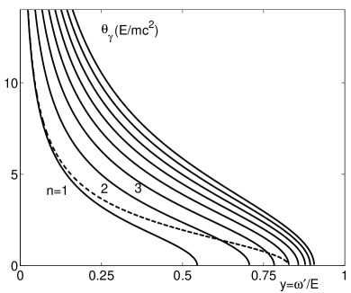
Figure 1: Photon scattering angles $\theta_{\gamma}$ for different harmonics $n$ versus the final photon energy $\omega^{\prime}$ at $x=4.8$ and $\xi^{2}=3$. The dashed curve corresponds to $\xi^{2}=0$.

Let us consider the azimuthal dependence of the detected Stokes parameters $\xi^{\prime}_{j}$ for the final photon. These parameters are defined with respect to the $x^{\prime}y^{\prime}z^{\prime}$-axes which are fixed to the scattering plane. The $x^{\prime}$-axis is the same as for the initial photon and perpendicular to the scattering plane:

$$x^{\prime}\;\parallel\;{\bf k}\times{\bf k}^{\prime};$$ (100)

the $y^{\prime}$-axis are in that plane:

$$y^{\prime}\;\parallel\;{\bf k}^{\prime}\times({\bf k}\times{\bf k}^{\prime})\,.$$ (101)

At small emission angles of the final photon $\theta_{\gamma}\ll 1$, the final photon moves almost along the direction of the $z$-axis and ${\bf k}\times{\bf k}^{\prime}$ azimuth is approximately equal to $\varphi+(3\pi/2)$. Let $\check{\xi}^{\prime}_{j}$ be the detected Stokes parameters for the final photons, fixed to the $xyz$-axes of the collider system. These Stokes parameters are connected with $\xi^{\prime}_{j}$ by the following relations:

$$\xi^{\prime}_{1} \approx -\check{\xi}^{\prime}_{1}\cos{2\varphi}+\check{\xi}^{\prime}_{3}\sin{2\varphi}\,,\;\;\xi^{\prime}_{2}=\check{\xi}^{\prime}_{2}\,,$$

$$\xi^{\prime}_{3} \approx -\check{\xi}^{\prime}_{3}\cos{2\varphi}-\check{\xi}^{\prime}_{1}\sin{2\varphi}\,.$$ (102)

Inserting these relations into the effective cross section, we find the Stokes parameters resulting from the scattering process itself and fixed to the $xyz$-axes of the collider system:

$$\check{\xi}^{\,(f)}_{1} \approx -{F_{1}\over F_{0}}\cos{2\varphi}-{F_{3}\over F_{0}}\sin{2\varphi}\,,\;\;\check{\xi}^{\,(f)}_{2}={F_{2}\over F_{0}}\,,$$

$$\check{\xi}^{\,(f)}_{3} \approx -{F_{3}\over F_{0}}\cos{2\varphi}+{F_{1}\over F_{0}}\sin{2\varphi}\,.$$ (103)

Note that (102) and (103) become exact in the limit $y\to y_{n}$.

It is not difficult to check that, for the considered case, the angle $\Delta\theta$ between vector $\mbox{\boldmath$\nu$}_{3}$ and ${\bf n}^{\prime}_{3}$ is very small:

$$\Delta\theta\approx|\mbox{\boldmath$\nu$}_{3\perp}-{\bf n}^{\prime}_{3\perp}|\approx{m\theta_{e}\over 2E^{\prime}}\leq{n\over\sqrt{1+\xi^{2}}}\,{\omega\over E^{\prime}}\,.$$ (104)

This means that the invariants $\zeta_{j}^{\prime}$ in (30) almost coincide with the projections $\mbox{\boldmath$\zeta$}^{\prime}\,\mbox{\boldmath$\nu$}_{j}$, defined in (84),

$$\zeta_{1}^{\prime} \approx \zeta^{\prime}_{\perp}\sin{(\varphi-\beta^{\prime})}\,,\;\;\zeta^{\prime}_{2}\approx\zeta^{\prime}_{\perp}\cos{(\varphi-\beta^{\prime})}\,,$$

$$\zeta^{\prime}_{3} \approx 2\lambda^{\prime}_{e}\,,$$ (105)

and that the exact equation (90) for the polarization of the final electron can be replaced with a high accuracy by the approximate equation

$$\mbox{\boldmath$\zeta$}^{(f)}\approx\sum_{j=1}^{3}\,{G_{j}\over F_{0}}\,\mbox{\boldmath$\nu$}_{j}\,.$$ (106)

Up to now we deal with the head-on collisions of the laser photon and the initial electron beams, when the collision angle $\alpha_{0}$ between the vectors ${\bf p}$ and $(-{\bf k})$ was equal zero. The detailed consideration of the case $\alpha_{0}\neq 0$ is given in Appendix B; see also Grin . We present here the summary of such a consideration. If $\alpha_{0}\neq 0$, the longitudinal component of the vector ${\bf k}$ becomes $k_{z}=-\omega\cos{\alpha_{0}}$ and it is appeared to be the transverse (to the momentum ${\bf p}$) component ${\bf k}_{\perp}$. However this transverse component is small, $|{\bf k}_{\perp}|\lesssim\omega\ll m$, therefore the transverse momenta of the final particles almost compensate each other, ${\bf p}_{\perp}^{\prime}={\bf k}_{\perp}-{\bf k}_{\perp}^{\prime}\approx-{\bf k}_{\perp}^{\prime}$. The invariants $x$ and $y$ become (compare with (97))

$$x\approx\frac{4E\omega}{m^{2}}\cos^{2}{\frac{\alpha_{0}}{2}},\;\;y\approx\frac{\omega^{\prime}}{E}\approx 1-\frac{E^{\prime}}{E}\,.$$ (107)

The polarization parameters of the initial and the final electrons and photons conserve their forms (78), (105),(40), (58), (102) and (103). Therefore, the whole dependence on $\alpha_{0}$ enters the effective cross section and the polarizations only via the quantity $x$ (107).

4.3 Averaged polarization of the final particles

The polarization of the final photon and electron, averaged over the azimuthal angle $\varphi$ in the collider system, is important in many application. To find it, one can use the same method as for the linear Compton scattering (see Khoze , GKPS83 , KPS98 ). Let us consider, for definiteness, the case of the circularly polarized laser photons. Substituting the exact equations (78) for $\zeta_{j}$ and the approximate equations (102), (105) for $\xi^{\prime}_{j}$, $\zeta^{\prime}_{j}$ into (33), we obtain the explicit dependence of the effective cross section (32) on $\varphi$. Then we take into account that the terms

$$\sum^{3}_{j=1}\,F_{j}^{(n)}\xi^{\prime}_{j} \approx \left(-F_{1}^{(n)}\,\cos{2\varphi}-F_{3}^{(n)}\,\sin{2\varphi}\right)\,\check{\xi}_{1}^{\prime}$$

$$+ F_{2}^{(n)}\check{\xi}^{\prime}_{2}+\left(F_{1}^{(n)}\,\sin{2\varphi}-F_{3}^{(n)}\,\cos{2\varphi}\right)\,\check{\xi}_{3}^{\prime}$$

after the averaging over $\varphi$ become equal to

$$\sum^{3}_{j=1}\,\langle F_{j}^{(n)}\xi^{\prime}_{j}\rangle\approx\langle F_{2}^{(n)}\rangle\,\check{\xi}^{\prime}_{2}$$ (109)

where

$$\langle F_{2}^{(n)}\rangle = \left({1\over 1-y}+1-y\right)\,c_{n}h_{n}P_{c}$$ (110)

$$+ y\left({2-y\over 1-y}\,f_{n}-{s^{2}_{n}\over 1+\xi^{2}}\,g_{n}\right)\zeta_{3}\,.$$

After a similar averaging of the terms $\sum_{j}G_{j}^{(n)}\zeta_{j}^{\prime}$, we obtain

$${d\sigma^{(n)}(\mbox{\boldmath$\zeta$},\,\mbox{\boldmath$\xi$},\,\mbox{\boldmath$\zeta$}^{\prime},\,\mbox{\boldmath$\xi$}^{\prime})\over dy}\approx{\pi r_{e}^{2}\over 2x}\;\left(\langle F_{0}^{(n)}\rangle+\langle F_{2}^{(n)}\rangle\,\check{\xi}^{\prime}_{2}\right.$$

$$\left.+G_{\perp}^{(n)}\mbox{\boldmath$\zeta$}_{\perp}\mbox{\boldmath$\zeta$}^{\prime}_{\perp}+G_{\parallel}^{(n)}\zeta_{3}^{\prime}+\sum^{3}_{i,j=1}\langle H_{ij}^{(n)}\,\zeta^{\prime}_{i}\,\xi^{\prime}_{j}\rangle\right)\,,$$ (111)

where $\langle F_{0}^{(n)}\rangle$, $G_{\perp}^{(n)}$ and $G_{\parallel}^{(n)}$ are given in (82), (50) and (3.2), respectively. According to the usual rules, we obtain from this equation the averaged polarization of the final particles for the case of the circularly polarized laser photons:

$$\langle\check{\xi}_{1}^{(n)(f)}\rangle \approx 0\,,\;\langle\check{\xi}_{2}^{(n)(f)}\rangle\approx{\langle F_{2}^{(n)}\rangle\over\langle F_{0}^{(n)}\rangle}\,,\;\;\langle\check{\xi}_{3}^{(n)(f)}\rangle\approx 0\,,$$

$$\langle\mbox{\boldmath$\zeta$}^{(n)(f)}_{\perp}\rangle \approx {G_{\perp}^{(n)}\over\langle F_{0}^{(n)}\rangle}\,\mbox{\boldmath$\zeta$}_{\perp}\,,\;\;\langle\zeta_{3}^{(n)(f)}\rangle\approx{G_{\parallel}^{(n)}\over\langle F_{0}^{(n)}\rangle}\,.$$ (112)

In a similar way we obtain the averaged polarization of the final particles for the case of the linearly polarized laser photons:

$$\langle\check{\xi}_{1}^{(n)(f)}\rangle \approx 0\,,\;\;\langle\check{\xi}_{2}^{(n)(f)}\rangle\approx{\langle F_{2}^{(n)}\rangle\over\langle F_{0}^{(n)}\rangle}\,,$$

$$\langle\check{\xi}_{3}^{(n)(f)}\rangle \approx {1\over\langle F_{0}^{(n)}\rangle}\,\left[2\langle\tilde{f}_{n}\rangle-(2+2c_{n}-s_{n}^{2}\Delta)\,\langle\tilde{g}_{n}\rangle\right.$$ (113)

$$+ \left.(1+c_{n})^{2}\,\langle\tilde{g}_{n}\cos{2\varphi}\rangle\right],$$

$$\langle\mbox{\boldmath$\zeta$}^{(n)(f)}_{\perp}\rangle \approx {\langle\tilde{G}_{\perp}^{(n)}\rangle\over\langle F_{0}^{(n)}\rangle}\,\mbox{\boldmath$\zeta$}_{\perp}\,,\;\;\langle\zeta_{3}^{(n)(f)}\rangle\approx{\langle\tilde{G}_{\parallel}^{(n)}\rangle\over\langle F_{0}^{(n)}\rangle}\,,$$

where $\langle F_{0}^{(n)}\rangle$, $\tilde{G}_{\perp}^{(n)}$, $\tilde{G}_{\parallel}^{(n)}$ are given in (83), (74), (75) and

$$\langle F_{2}^{(n)}\rangle=y\left({2-y\over 1-y}\,\langle\tilde{f}_{n}\rangle-{s^{2}_{n}\over 1+\xi^{2}}\,\langle\tilde{g}_{n}\rangle\right)\,\zeta_{3}\,.$$ (114)

Note that the averaged Stokes parameters of the final photon do not depend on $\mbox{\boldmath$\zeta$}_{\perp}$ and that the averaged polarization vector of the final electron is not equal zero only if $P_{c}\neq 0$ or if $\mbox{\boldmath$\zeta$}\neq 0$. These properties are similar to those in linear Compton scattering.

5 Limiting cases

In this section we consider several limiting cases in which description of the non-linear Compton scattering is essentially simplified.

(i). The case of $\;\xi^{2}\to 0$. At small $\xi^{2}$ all harmonics with $n>1$ disappear due to the properties (43), (45), (68), (69) and we have

$$d\sigma^{(n)}(\mbox{\boldmath$\zeta$},\,\mbox{\boldmath$\xi$},\,\mbox{\boldmath$\zeta$}^{\prime},\,\mbox{\boldmath$\xi$}^{\prime})\propto\xi^{2(n-1)}\;\;\mbox{ at }\;\;\xi^{2}\to 0\,.$$ (115)

We have checked that in this limit our expression for the effective cross section of the first harmonic, $d\sigma^{(1)}$, coincides with the result known for the linear Compton effect; see Appendix A.

(ii). The case of $\;y\to 0$ for arbitrary $x$ and $\xi^{2}$. This limit corresponds to forward scattering ($\theta_{e}=0\,,\;\theta_{\gamma}=\pi$). We expect that in this limit an electron as well as a photon does not change its polarization. Indeed, at small $y$ all harmonics with $n>1$ disappear due to the properties (43), (45) and (68), (69), i.e.

$$d\sigma^{(n)}(\mbox{\boldmath$\zeta$},\,\mbox{\boldmath$\xi$},\,\mbox{\boldmath$\zeta$}^{\prime},\,\mbox{\boldmath$\xi$}^{\prime})\propto y^{n-1}\;\;\mbox{ at }\;\;y\to 0\,,$$ (116)

and we found that

$$F_{0}=2\,,\;\;F_{j}=2\xi_{j}\,,\;\;G_{j}=2\zeta_{j}\,,\;\;H_{ij}=2\zeta_{i}\,\xi_{j}\,,$$ (117)

therefore,

$${d\sigma(\mbox{\boldmath$\zeta$},\,\mbox{\boldmath$\xi$},\,\mbox{\boldmath$\zeta$}^{\prime},\,\mbox{\boldmath$\xi$}^{\prime})\over dy\,d\varphi}={r_{e}^{2}\over 2x}\,(1+\mbox{\boldmath$\zeta$}\mbox{\boldmath$\zeta$}^{\prime})(1+\mbox{\boldmath$\xi$}\mbox{\boldmath$\xi$}^{\prime})$$ (118)

It follows from this equation that

$$\mbox{\boldmath$\zeta$}^{(f)}=\mbox{\boldmath$\zeta$}\,,\;\;\mbox{\boldmath$\xi$}^{(f)}=\mbox{\boldmath$\xi$}\,,$$ (119)

in accordance with our expectation.

Note that for the case of circularly polarized laser photons the equations, similar to (119), hold also for each harmonic separately: $\mbox{\boldmath$\zeta$}^{(n)(f)}=\mbox{\boldmath$\zeta$}\,,\;\;\mbox{\boldmath$\xi$}^{(n)(f)}=\mbox{\boldmath$\xi$}$.

(iii). The case of $\;x\to 0$ for arbitrary $\xi^{2}$, which corresponds to the classical limit. In this limit an electron does not change its polarization. For a certain harmonic with $n\,x\ll 1$ one has $y\leq y_{n}<nx\ll 1$ and

$$G_{j}^{(n)}=F_{0}^{(n)}\,\zeta_{j}\,,\;\;H_{ij}^{(n)}=\zeta_{i}\,F_{j}^{(n)}\,,$$ (120)

therefore, in this limit the effective cross section both for the circularly and linearly polarized laser photons has the form

$${d\sigma^{(n)}(\mbox{\boldmath$\zeta$},\,\mbox{\boldmath$\xi$},\,\mbox{\boldmath$\zeta$}^{\prime},\,\mbox{\boldmath$\xi$}^{\prime})\over dy\,d\varphi}$$ (121)

$$={r_{e}^{2}\over 4x}\,\left(F_{0}^{(n)}+\sum_{j=1}^{3}\,F_{j}^{(n)}\,\xi_{j}^{\prime}\right)\,\left(1+\sum_{i=1}^{3}\,\zeta_{i}\zeta^{\prime}_{i}\right)\,.$$

As a consequence, the polarization of the final electron for a given harmonic $n$ is

$$\mbox{\boldmath$\zeta$}^{(n)(f)}=\sum_{i=1}^{3}\,\zeta_{i}\,{\bf n}^{\prime}_{i}\,,$$ (122)

where the unit vectors ${\bf n}^{\prime}_{i}$ are defined in (30). To show that $\mbox{\boldmath$\zeta$}^{(n)(f)}$ coincides with $\zeta$, one has to demonstrate that the unit vectors ${\bf n}^{\prime}_{i}$ coincide with the unit vectors ${\bf n}_{i}$ from (27). This can be easily seen, for example, in the frame of reference in which ${\bf p}=0$ and in which the photon energies are small in the considered limit, $\omega^{\prime}<n\omega\ll m$, as well as the momentum of the final electron, $|{\bf p}^{\prime}|\ll m$. As a result,

$$\mbox{\boldmath$\zeta$}^{(n)(f)}=\mbox{\boldmath$\zeta$}\,,$$ (123)

in accordance with our expectation.

(iv). The case of $\;\theta_{\gamma}\to 0$ for the circularly polarized laser photons, $P_{c}=\pm 1$. At small $\theta_{\gamma}$ the energy of the final photon is close to its maximum, $y\to y_{n}$, and the functions (41) become equal to

$$f_{n} = g_{n}=h_{n}=\gamma_{n}\,\left(y_{n}-y\right)^{n-1}\,,$$ (124)

$$\gamma_{n} = (n^{n}/n!)^{2}\,\left[{\xi^{2}\over y_{n}(1-y_{n})(1+\xi^{2})}\right]^{n-1}\,.$$

Therefore, all harmonics with $n>1$ disappear and only the photons of the first harmonic can be emitted along the direction of the initial electron beam:

$${d\sigma^{(n)}(\mbox{\boldmath$\zeta$},\,\mbox{\boldmath$\xi$},\,\mbox{\boldmath$\zeta$}^{\prime},\,\mbox{\boldmath$\xi$}^{\prime})\over dyd\varphi} = {r^{2}_{e}\over 4x}\,F^{(n)}\propto f_{n}\propto(y_{n}-y)^{n-1}$$ (125)

$$\mbox{ at }\;\;y\to y_{n}\,,$$

with

$${F^{(n)}\over f_{n}} = {2-2y_{n}+y_{n}^{2}\over 1-y_{n}}\,(1+\zeta_{3}\zeta_{3}^{\prime})(1-P_{c}\xi_{2}^{\prime})$$

$$- {y_{n}(2-y_{n})\over 1-y_{n}}\,(\zeta_{3}+\zeta_{3}^{\prime})(P_{c}-\xi_{2}^{\prime})$$

$$+ 2(\mbox{\boldmath$\zeta$}_{\perp}\mbox{\boldmath$\zeta$}^{\prime}_{\perp})(1-P_{c}\xi_{2}^{\prime})\,.$$

In this limit, the final photons are circularly polarized,

$$\xi_{1}^{(n)(f)}=0\,,\;\;\xi_{2}^{(n)(f)}=-P_{c}\,,\;\;\xi_{3}^{(n)(f)}=0\,,$$ (127)

and the polarization of the final electrons is

$$\mbox{\boldmath$\zeta$}_{\perp}^{(n)(f)} = {2(1-y_{n})\over 2-(2y_{n}-y_{n}^{2})(1+\zeta_{3}P_{c})}\,\mbox{\boldmath$\zeta$}_{\perp}\,,$$ (128)

$$\zeta_{3}^{(n)(f)} = {2\zeta_{3}-(2y_{n}-y_{n}^{2})(\zeta_{3}+P_{c})\over 2-(2y_{n}-y_{n}^{2})(1+\zeta_{3}P_{c})}\,,$$

in particular, at $\zeta_{3}=\pm 1$ the helicity of the electron is conserved in the non-linear Compton scattering, $\zeta_{3}^{(n)(f)}(y\to y_{n})\to\zeta_{3}$. Note that the function $F^{(n)}$ does not depend on the azimuthal angle $\varphi$ and (127) and (128) are in accordance with the results (112) for the polarizations averaged over $\varphi$.

Let us consider in more detail this limit for the first harmonic. The spectrum of the fist harmonic,

$${d\sigma^{(1)}(\mbox{\boldmath$\zeta$},\,\mbox{\boldmath$\xi$})\over dy} = {2\pi r^{2}_{e}\over x(1-y_{1})}[2-(2y_{1}-y_{1}^{2})(1+\zeta_{3}P_{c})]$$ (129)

$$\mbox{ at }\;y\to y_{1}\,,$$

depends on the non-linearity parameter $\xi^{2}$ only via

$$y_{1}={x\over x+1+\xi^{2}}\,.$$

For the case of “good polarization”, $\zeta_{3}P_{c}=-1$, the first harmonic has a peak at $y\to y_{1}$ of the value

$${d\sigma^{(1)}(\mbox{\boldmath$\zeta$},\,\mbox{\boldmath$\xi$})\over dy} = {4\pi r^{2}_{e}\over x}\,\left(1+{x\over 1+\xi^{2}}\right)$$ (130)

$$\mbox{ at }\;\;y\to y_{1}\;\;\mbox{ and }\;\;\zeta_{3}P_{c}=-1\,.$$

At large $x\gg 1+\xi^{2}$ the quantity $y_{1}$ tends to $1$,

$$1-y_{1}={1+\xi^{2}\over x+1+\xi^{2}}\ll 1\,,$$ (131)

and the function $F^{(1)}$ becomes large

$$F^{(1)} = {1\over 1-y_{1}}\,\left[(1+\zeta_{3}\zeta_{3}^{\prime})(1-P_{c}\xi_{2}^{\prime})\right.$$ (132)

$$- \left.(\zeta_{3}+\zeta_{3}^{\prime})(P_{c}-\xi_{2}^{\prime})\right]\,.$$

Therefore, integrating the effective cross section for the first harmonic, $d\sigma^{(1)}\propto 1/(1-y)$, near its maximum, i.e. in the region

$${1+\xi^{2}\over x}\ll 1-y\ll 1\,,$$ (133)

we find (with logarithmic accuracy) the total cross section

$$\sigma(\mbox{\boldmath$\zeta$},\,\mbox{\boldmath$\xi$},\,\mbox{\boldmath$\zeta$}^{\prime},\,\mbox{\boldmath$\xi$}^{\prime}) = {\pi r_{e}^{2}\over 2x}\,\left[(1+\zeta_{3}\zeta_{3}^{\prime})(1-P_{c}\xi_{2}^{\prime})\right.$$ (134)

$$- \left.(\zeta_{3}+\zeta_{3}^{\prime})(P_{c}-\xi_{2}^{\prime})\right]\,\ln{x\over 1+\xi^{2}}\,.$$

If one sums this expression over spin states of the final particles, one arrives at the result for the cross section

$$\sigma(\mbox{\boldmath$\zeta$},\,\mbox{\boldmath$\xi$})={2\pi r_{e}^{2}\over x}\,\left(1-\zeta_{3}P_{c}\right)\,\ln{x\over 1+\xi^{2}}\,,$$ (135)

which is in accordance with that obtained by a different method in BKMS .

(v). The case of $\;\theta_{\gamma}\to 0$ for the linearly polarized laser photons. At $y\to y_{n}$, the argument $a$ tends to zero, while the argument $b$ tends to the nonzero constant, $b\to n\xi^{2}/[2(1+\xi^{2})]$; the function $A_{0}(n,\,a,\,b)\propto\sqrt{y_{n}-y}$ vanishes for odd $n$ and $A_{0}(n,\,a,\,b)\to(-1)^{n/2}J_{n/2}(b)$ for even $n$. As a result, the spectra and the polarizations are different in this limit for odd and even harmonics.

Odd harmonics. The spectrum in this case,

$${d\sigma^{(n)}(\mbox{\boldmath$\zeta$},\,\mbox{\boldmath$\xi$})\over dy} = {2\pi r^{2}_{e}\over x(1-y_{n})}\,\left(2-2y_{n}+y_{n}^{2}\right)$$

$$\times \left[J_{(n-1)/2}(b)-J_{(n+1)/2}(b)\right]^{2}\;\mbox{ at }\;\;y\to y_{n}\,,$$

depends on the non-linearity parameter $\xi^{2}$ via $y_{n}$ and via the argument $b$, but the spectrum does not depend on the initial electron polarization. In this limit, the final photons have circular polarization, proportional to $\zeta_{3}$, and linear polarization along the direction of the linear polarization of the laser photons,

$$\check{\xi}_{1}^{(n)(f)} = 0\,,\;\;\check{\xi}_{2}^{(n)(f)}={2y_{n}-y^{2}_{n}\over 2-2y_{n}+y_{n}^{2}}\,\zeta_{3}\,,$$

$$\check{\xi}_{3}^{(n)(f)} = {2(1-y_{n})\over 2-2y_{n}+y_{n}^{2}}\,.$$ (137)

The polarization of the final electrons in this case is

$$\mbox{\boldmath$\zeta$}_{\perp}^{(n)(f)} = {2(1-y_{n})\over 2-2y_{n}+y_{n}^{2}}\,\mbox{\boldmath$\zeta$}_{\perp}\,,$$ (138)

$$\zeta_{3}^{(n)(f)} = \zeta_{3}\,,$$

in particular, the final electrons have the same mean helicity as that for the initial one.

Even harmonics. The spectrum reads

$${d\sigma^{(n)}(\mbox{\boldmath$\zeta$},\,\mbox{\boldmath$\xi$})\over dy} = {2\pi r^{2}_{e}\over x(1-y_{n})}\,{2y_{n}^{2}\over\xi^{2}}\,\left[J_{n/2}(b)\right]^{2}$$ (139)

$$\mbox{ at }\;\;y\to y_{n}\,.$$

In this limit the final photons have only circular polarization equals to $\zeta_{3}$, and the final electrons have mean helicity opposite to that for the initial one:

$$\check{\xi}_{1}^{(n)(f)}=0\,,\;\;\check{\xi}_{2}^{(n)(f)}=\zeta_{3}\,,\;\;\check{\xi}_{3}^{(n)(f)}=0\,,$$ (140)

$$\mbox{\boldmath$\zeta$}_{\perp}^{(n)(f)}=0\,,\;\;\zeta_{3}^{(n)(f)}=-\zeta_{3}\,.$$

Note that (137), (138) and (140) are in accordance with the results (113) for the polarizations averaged over $\varphi$.

6 Numerical results related to $\gamma\gamma$ and $\gamma e$ colliders

In this section we present some examples which illustrate the dependence of the differential cross sections and the polarizations, obtained in the previous sections, on the final photon energy. We restrict ourselves to properties of the high-energy photon beam which are of most importance for the future $\gamma\gamma$ and $\gamma e$ colliders. The used parameters are close to those in the TESLA projectTESLA . In particular,

$$x\approx 4E\omega/m^{2}=4.8\,,$$

and the non-linearity parameter $\xi^{2}$ (5) is chosen either the same as in the TESLA project, $\xi^{2}=0.3$, or larger by one order of magnitude, $\xi^{2}=3$, just to illustrate the tendencies. In figures below we use notation

$$\sigma_{0}=\pi r_{e}^{2}\approx 2.5\cdot 10^{-25}\;\;\mbox{cm}^{2}\,.$$

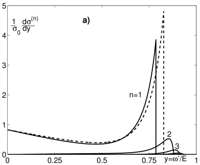
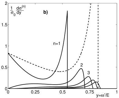
Figure 2: Energy spectra of final photons for different harmonics $n$ at $\zeta_{3}\,P_{c}=-1$ and: (a) $\xi^{2}=0.3$;   (b) $\xi^{2}=3$. The dashed curves correspond to $\xi^{2}=0$.

Figure 3: Mean helicity of the final photons for different harmonics $n$ versus the final photon energy $\omega^{\prime}$ at $P_{c}=-1,\;\zeta_{3}=1$ and $\xi^{2}=3$. The dashed curve corresponds to $\xi^{2}=0$.

The case of the circularly polarized laser photons (Figs. 2, 3, 4, 5).

The spectra of the few first harmonics are shown in Fig. 2 for the case of “a good polarization”, when helicities of the laser photon and the initial electron are opposite, $\zeta_{3}P_{c}=-1$. At a small intensity of the laser wave ($\xi^{2}=0.3$, Fig. 2a) the main contribution is given by photons of the first harmonic and the probability for generation of the higher harmonics is small. However, with the growth of the non-linearity parameter ($\xi^{2}=3$, Fig. 2b), the maximum energy for the first harmonic decreases and the peak of this harmonic at $y=y_{1}$ (see Eq. (130)) decreases as well. As for the higher harmonics, with the rise of $\xi^{2}$ (Fig. 2b) we see an increase of the yield of photons with energies higher than the maximum energy of the first harmonic. As a result, the total spectrum becomes considerable wider.

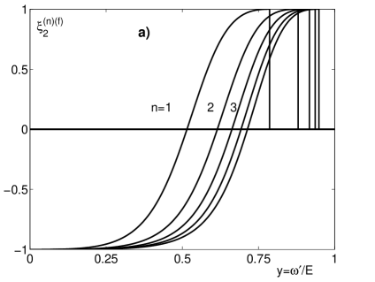
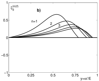
Figure 4: The Stokes parameters of final photons for different harmonics $n$ versus the final photon energy $\omega^{\prime}$ at $\zeta_{3}=1,\;P_{c}=-1$, $\xi^{2}=0.3$: (a) the mean helicity $\xi_{2}^{(n)(f)}$;   (b) the linear polarization $\xi_{3}^{(n)(f)}$ transverse to the scattering plane. The Stokes parameter obeys $\xi_{1}^{(n)(f)}=0$ in this case.

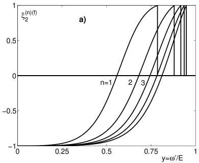
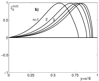
Figure 5: The same as in Fig. 4, but for $\zeta_{1}=0,\;\zeta_{2}=0.7$ and $\zeta_{3}=0.7$.

The mean helicities of the final photons for the few first harmonics, $\xi_{2}^{(n)(f)}$, are shown in Fig. 3 and Figs. 4a, 5a. In Fig. 3 we compare the two cases $\xi^{2}=3$ and $\xi^{2}=0$. Each harmonic is 100% polarized near its maximum $y=y_{n}$, therefore, the whole $\gamma$ beam at $x>0.5$ has a high degree of circular polarization. However, for linear Compton scattering, the final photon in the region of high energies, $y\geq 0.8$, is almost 100 % circularly polarized, while for the non-linear case $\xi^{2}=3$, only harmonics with $n\geq 4$ contribute in this energy range. But the cross sections corresponding to these harmonics are small (see Fig. 2b).

There is an interesting feature related to the linear polarization of the final photons; see Figs 4b and 5b. Such a polarization is described by the Stokes parameters $\xi_{1}^{(n)(f)}$ and $\xi_{3}^{(n)(f)}$. These parameters averaged over the azimuthal angle $\varphi$ (see (112)) vanish. On the other hand, the degree of the linear polarization for a given angle $\varphi$ may be close to 100%, especially in the case when the initial electron has a transverse polarization as well (see Fig. 5b). It is not excluded that this property of our process may result in a sizable dependence of the luminosities of $\gamma\gamma$ collisions at a photon collider on the mutual orientation (parallel or perpendicular) of the linear polarizations of the colliding photons. Such a dependence is of importance, for example, for the study of a Higgs boson production at a $\gamma\gamma$ collider. As far as we know, this possibility has not been discussed so far even for linear Compton scattering.

The case of the linearly polarized laser photons (Figs. 6, 7, 8).

The spectra of the first few harmonics for this case are shown in Fig. 6. They differ considerably from those for the case of the circularly polarized laser photons shown in Fig. 2. First of all, in the considered case the spectra do not depend on the polarization of the initial electrons. The maximum of the first harmonic at $y=y_{1}$ now is about two times smaller than that on Fig. 2. Besides, the harmonics with $n>1$ do not vanish at $y=y_{n}$ contrary to such harmonics on Fig. 2.

For the first few harmonics the mean helicities of the final photons, $\xi_{2}^{(n)(f)}$, are shown at $\zeta_{3}=1$ in Fig. 7a for $\xi^{2}=0.3$ and in Fig. 7b for $\xi^{2}=3$. We would like to direct attention to the surprising fact that each harmonic is almost 100% circularly polarized near the high-energy part of the spectrum. The curves on Fig. 7 are given for the azimuthal angle $\varphi=0$, for other values of $\varphi$ these curves would look a bit different, but not too much.

The degree of linear polarization of the final photons is not large in the high-energy part of the spectrum, but it becomes rather high in the middle and the low part of the spectrum; see Fig. 8. Certainly, the direction of this polarization depends on the azimuthal angle $\varphi$, as the result the linear polarization averaged over $\varphi$ is substantially smaller, see Fig. 9, than one on Fig. 8. Nevertheless, the non-trivial effects, related to the high degree of linear polarization present at a certain $\varphi$, do exist. For example, it was shown PST2003 that for linear Compton scattering this feature leads to an important effect for the luminosity of $\gamma\gamma$ collisions.

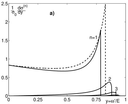
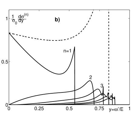
Figure 6: Energy spectra of final photons for different harmonics $n$ in the case of the linearly polarized laser photons and: (a) $\xi^{2}=0.3$;   (b) $\xi^{2}=3$. The dashed curves correspond to $\xi^{2}=0$.

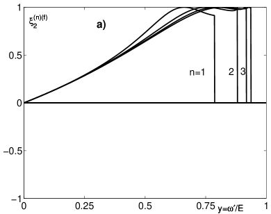
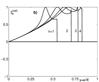
Figure 7: The mean helicity $\xi_{2}^{(n)(f)}$ of the final photons for different harmonics $n$ versus the final photon energy $\omega^{\prime}$ at $\zeta_{3}=1$ and: (a) $\xi^{2}=0.3$;   (b) $\xi^{2}=3$. The laser photons are linearly polarized. The scattering plane is parallel to the direction of the laser photon polarization.

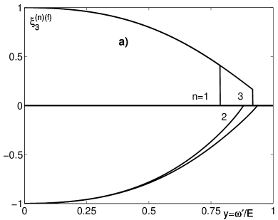
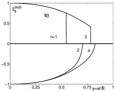
Figure 8: The Stokes parameters $\xi_{3}^{(n)(f)}$ of the final photons for different harmonics $n$ versus the final photon energy $\omega^{\prime}$ at: (a) $\xi^{2}=0.3$;   (b) $\xi^{2}=3$. The laser photons are linearly polarized. The scattering plane is perpendicular to the direction of the laser photon polarization. The Stokes parameter obeys $\xi_{1}^{(n)(f)}=0$ in this case.

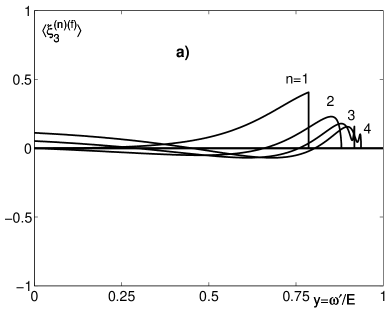
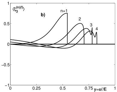
Figure 9: The Stokes parameters $\langle\xi_{3}^{(n)(f)}\rangle$ of the final photons for different harmonics $n$, averaged over the azimuthal angle $\varphi$, versus the final photon energy $\omega^{\prime}$ at: (a) $\xi^{2}=0.3$;   (b) $\xi^{2}=3$. The laser photons are linearly polarized. The averaged Stokes parameter $\langle\xi_{1}^{(n)(f)}\rangle=0$ in this case.

7 Summary and comparison with other papers

Our main results are given by (46)–(52) for circularly and by (71)–(76) for linearly polarized laser beam. They are expressed in terms of the 16 functions $F_{0},\;F_{j},\;G_{j}$ and $H_{ij}$ with $i,\,j=1\div 3$, which describe completely the polarization properties of the non-linear Compton scattering in a compact invariant form. The functions $F_{0}$ and $F_{j}$ enter the total cross section (34), (81), the differential cross sections (80), (81) and the Stokes parameters of the final photons (35). The polarization of the final electrons is described by functions $G_{j}$, which enter the polarization vector $\mbox{\boldmath$\zeta$}^{(f)}$ given by the exact equations (37), (90) and the approximate equations (106).

Besides, we considered the kinematics and the approximate formulae relevant for the problem of $e\to\gamma$ conversion at the $\gamma\gamma$ and $\gamma e$ colliders. In particular, we discuss the polarization of the final photons and electrons averaged over the azimuthal angle $\varphi$ (see (112), (113)) and the spectra and the polarization of the final particles in the limit of small and large energies of the final photons (Sect. 5). For circularly polarized laser photons and for large values of the parameter $x\gg 1+\xi^{2}$, we obtain (with logarithmic accuracy) the simple analytical expression for the total cross section (134). In Sect. 6 we present the numerical results and discuss several interesting features in the final photon polarization, which may be useful for the analysis of the luminosity of $\gamma\gamma$ collisions.

Let us compare our results with those obtained earlier.

Circular polarization of laser photons. In the literature we found the results which can be compared with our functions $F_{0},F_{2}$ and $G_{j}$, namely, in NR-review (the function $F_{0}$ only at $\zeta_{j}=0$), in GS ; Tsai ; Yokoya (the functions $F_{0}$ and $F_{2}$ only at $\zeta_{1}=\zeta_{2}=0$) and in BPM (the function $F_{0}$ for arbitrary $\zeta_{j}$). For these cases our results coincide with the above mentioned ones. For polarization of the final electron, our results differ slightly from those in Yokoya ; BPM . Namely, the function $G_{2}$ at $\zeta_{1}=\zeta_{2}=0$ given in Yokoya and the functions $G_{j}$ for arbitrary $\zeta_{j}$ obtained in BPM coincide with ours. However, the polarization vector $\mbox{\boldmath$\zeta$}^{(f)}$ in the collider system is obtained in papers Yokoya ; BPM only in the approximate form equivalent to our approximate equation (106).

Linear polarization of laser photons. For this case we found in the literature the expressions which can be compared with ours functions $F_{0},F_{1},\,F_{2},\,F_{3}$. The results in  NR-review are in agreement with our function $F_{0}$ (71), and the results in GR are in agreement with our functions $F_{j}$ (3.3).

The correlation of the final particles’ polarizations are described by the functions $H_{ij}$ given in (52), (76). We did not find in the literature any results for these functions both for the case of the circular and the linear polarization.

Appendix A: Limit of the weak laser field

At $\xi^{2}\to 0$, the cross section (32) has the form

$$d\sigma(\mbox{\boldmath$\zeta$},\,\mbox{\boldmath$\xi$},\,\mbox{\boldmath$\zeta$}^{\prime},\,\mbox{\boldmath$\xi$}^{\prime})={r_{e}^{2}\over 4x}\;F\;d\Gamma\,,$$ (141)

$$d\Gamma=\delta(p+k-p^{\prime}-k^{\prime})\;{d^{3}k^{\prime}\over\omega^{\prime}}{d^{3}p^{\prime}\over E^{\prime}}\,,$$

where

$$F=F_{0}+\sum^{3}_{j=1}\left(F_{j}\xi^{\prime}_{j}\;+\;G_{j}\zeta^{\prime}_{j}\right)+\sum^{3}_{i,j=1}H_{ij}\,\zeta^{\prime}_{i}\,\xi^{\prime}_{j}\,.$$ (142)

To compare it with the cross section for linear Compton scattering, we should take into account that the Stokes parameters of the initial photon have the values (40) for the circular polarization and the values (58) for the linear polarization. Besides, our invariants $c_{1}$, $s_{1}$, $r_{1}$ and the auxiliary functions (70) transform at $\xi^{2}\to 0$ to

$$c_{1} \to c=1-2r\,,\;\;s_{1}\to s=2\sqrt{r(1-r)}\,,$$

$$r_{1} \to r={y\over x(1-y)}\,,$$ (143)

$$X_{1} \to -c\,,\;\;Y_{1}\to c(1-\xi_{3})\,,\;\;V_{1}\to-\xi_{3}\,.$$

Our functions

$$F_{0} = {1\over 1-y}+1-y-s^{2}(1-\xi_{3})$$

$$- y\left(s\,\zeta_{2}-{2-y\over 1-y}c\,\zeta_{3}\right)\xi_{2}\,,$$

$$F_{1} = 2c\xi_{1}+{y\over 1-y}s\,\zeta_{1}\,\xi_{2}\,,$$ (144)

$$F_{2} = \left({1\over 1-y}+1-y\right)\,c\,\xi_{2}-{ysc}\,\zeta_{2}$$

$$+ y\left({2-y\over 1-y}\,-s^{2}\right)\zeta_{3}-ys\,\zeta_{1}\xi_{1}+ys\left(c\zeta_{2}+s\zeta_{3}\right)\,\xi_{3}\,,$$

$$F_{3} = s^{2}-{y\over 1-y}s\,\zeta_{2}\,\xi_{2}+(1+c^{2})\,\xi_{3}$$

coincide with those in GKPS83 . Our functions

$$G_{1} = (1+c^{2}+s^{2}\xi_{3})\zeta_{1}-{y\over 1-y}s\,\zeta_{3}\,\xi_{1}\,,$$ (145)

$$G_{2} = -{ys\over 1-y}\xi_{2}+(1+c^{2}+s^{2}\xi_{3})\;\zeta_{2}-{ysc\over 1-y}\,(1-\xi_{3})\;\zeta_{3}\,,$$

$$G_{3} = yc\,{2-y\over 1-y}\xi_{2}+ys\zeta_{1}\xi_{1}+ysc(1-\xi_{3})\;\zeta_{2}$$

$$+ \left[1+\left({1\over 1-y}-y\right)\,(c^{2}+s^{2}\xi_{3})\right]\;\zeta_{3}$$

coincide with the functions $\Phi_{j}$ given by Eqs. (31) in KPS98 . Finally, we check that our functions

$$H_{11} = ys\xi_{2}+{2-2y+y^{2}\over 1-y}\,c\,\zeta_{1}\,\xi_{1}$$

$$+ y\left[{2-y\over 1-y}\,\xi_{3}+s^{2}(1-\xi_{3})\right]\,\zeta_{2}-ysc(1-\xi_{3})\,\zeta_{3}\,,$$

$$H_{21} = -\frac{y}{1-y}\left[s^{2}+(1-y+c^{2})\xi_{3}\right]\zeta_{1}$$

$$+ {2-2y+y^{2}\over 1-y}\,c\xi_{1}\zeta_{2}-ys\xi_{1}\zeta_{3}\,,$$

$$H_{31} = \frac{ycs}{1-y}\,(1-\xi_{3})\zeta_{1}+\frac{ys}{1-y}\,\xi_{1}\zeta_{2}+2c\xi_{1}\zeta_{3}\,,$$

$$H_{12} = 2c\zeta_{1}\xi_{2}-{ys\over 1-y}\,\xi_{1}\,,$$ (146)

$$H_{22} = -\frac{ycs}{1-y}\,(1-\xi_{3})+2c\,\zeta_{2}\,\xi_{2}-\frac{ys}{1-y}\,\zeta_{3}\,\xi_{2}\,,$$

$$H_{32} = \frac{y}{1-y}\left[2-y-s^{2}(1-\xi_{3})\right]+ys\,\zeta_{2}\,\xi_{2}$$

$$+ \frac{2-2y+y^{2}}{1-y}c\,\zeta_{3}\,\xi_{2}\,,$$

$$H_{13} = s^{2}\,\zeta_{1}+\left(1+c^{2}+\frac{y^{2}}{1-y}\right)\,\xi_{3}\zeta_{1}$$

$$- yc\,{2-y\over 1-y}\,\xi_{1}\,\zeta_{2}-ys\,\xi_{1}\zeta_{3}\,,$$

$$H_{23} = -ys\,\xi_{2}+y\frac{2-y}{1-y}\,c\,\xi_{1}\,\zeta_{1}+\frac{1-y+y^{2}}{1-y}\,s^{2}\,\zeta_{2}$$

$$+ \left(1+c^{2}+\frac{y^{2}c^{2}}{1-y}\right)\,\xi_{3}\zeta_{2}+ysc(1-\xi_{3})\,\zeta_{3}\,,$$

$$H_{33} = \frac{ys}{1-y}\,\xi_{1}\,\zeta_{1}-\frac{ysc}{1-y}\,(1-\xi_{3})\,\zeta_{2}$$

$$+ s^{2}\,\zeta_{3}+(1+c^{2})\,\xi_{3}\,\zeta_{3}$$

coincide with the corresponding functions in Grozin . Making such a comparison, one has to take into account that the set of unit 4-vectors used in our paper (see (19), (22)), and one used in paper Grozin are different. The relations between our notation and the notation of Grozin , which are marked below by super-index $G$, are the following:

$$\xi_{1,3}^{G} = -\xi_{1,3}\,,\;\;\xi_{2}^{G}=\xi_{2}\,,\;\;\xi_{1,3}^{{}^{\prime}G}=-\xi^{\prime}_{1,3}\,,\;\;\xi_{2}^{{}^{\prime}G}=\xi^{\prime}_{2}\,,$$

$$\zeta_{1,3}^{G} = \zeta_{3,1}\,,\;\;\zeta_{2}^{G}=-\zeta_{2}\,,$$ (147)

$$\zeta_{1}^{{}^{\prime}G} = c\zeta_{3}^{\prime}-s\zeta_{2}^{\prime}\,,\;\;\zeta_{2}^{{}^{\prime}G}=-c\zeta_{2}^{\prime}-s\zeta_{3}^{\prime}\,,\;\;\zeta_{3}^{{}^{\prime}G}=\zeta_{1}^{\prime}\,.$$

Besides, in Grozin there is a misprint, namely, the factor $1/4$ should be inserted in the right-hand-side of the equation, which is analogous to our (141).

Appendix B:
The case of nonzero beam collision angle

In this appendix we consider the case when the beam collision angle $\alpha_{0}$ between the vectors ${\bf p}$ and $(-{\bf k})$ is not equal to zero. We omit systematically terms of the order of $\omega/m$, $m/E$, $\theta_{\gamma}$ and $\theta_{e}$. In this approximation the vectors (19) take the form

$${\bf e}_{\perp}^{(1)} = {{\bf p}\times{\bf p}^{\prime}\over|{\bf p}\times{\bf p}^{\prime}|}\,,\;\;\;{\bf e}_{\perp}^{(2)}=-{{\bf k}^{\prime}_{\perp}\over|{\bf k}^{\prime}_{\perp}|}\,,$$

$$e_{0}^{(j)} = e_{z}^{(j)}={{\bf e}_{\perp}^{(j)}{\bf k}_{\perp}\over(1+\cos{\alpha_{0}})\,\omega}\,,$$ (148)

$$e^{(i)}\,e^{(j)} = -{\bf e}_{\perp}^{(i)}\,{\bf e}_{\perp}^{(j)}=-\delta_{ij}\,,$$

i.e. the transverse components ${\bf e}_{\perp}^{(j)}$ do not differ from their values at $\alpha_{0}=0$, and zero and the $z$-components of $e^{(j)}$ vanish in the limit ${\bf k}_{\perp}\to 0$. As a consequence, the vector

$${\bf e}_{{\rm L}\perp}={\bf e}_{\perp}^{(1)}\,\sin{\varphi}-{\bf e}_{\perp}^{(2)}\,\cos{\varphi}$$ (149)

also does not differ from its value at $\alpha_{0}=0$. This means that the parameter $\varphi$ in all the equations of Subsect. 3.3 is the same azimuthal angle of the final photon counted from the $x$-axis chosen along the direction of the vector ${\bf e}_{{\rm L}\perp}$. Therefore, the Stokes parameters of the laser photons conserve their values (40), (58).

The Stokes parameters of the final photons are determined with respect to the transverse to the vector ${\bf k}^{\prime}$ components of the polarization 4-vectors $e^{(1)}$ and $(-e^{(2)})$. At small emission angles $\theta_{\gamma}\ll 1$, the final photon moves almost along the direction of the $z$-axis and, therefore, the components of $e^{(j)}$, which are transverse to the momentum ${\bf k}^{\prime}$, coincide within the used accuracy with the vectors ${\bf e}_{\perp}^{(j)}$ from (148). This means that the Stokes parameters of the final photons also conserve their forms (102), (103).

At last, using (148) it is not difficult to check that the polarization parameters of the electrons $\zeta_{j}$ and $\zeta_{j}^{\prime}$, defined by (25), (26) and (30), conserve their forms (78) and (105). Therefore, the whole dependence on $\alpha_{0}$ enters into the effective cross section and the polarizations only via the quantity $x=(4E\omega/m^{2})\,\cos^{2}{(\alpha_{0}/2)}$.

Finally, one needs to discuss the relation between the direction of the laser wave linear polarization and the angle $\varphi$ which enters (149) and the equations in Sect. 3.3. Let us decompose the vector ${\bf e}_{\rm L}$ along the photon momentum ${\bf k}$ and in the plane orthogonal to that momentum:

$${\bf e}_{\rm L}={\tilde{\bf e}}_{\rm L}+c{\bf k}\,,\;\;{\tilde{\bf e}}_{\rm L}{\bf k}=0\,.$$ (150)

It is important to note that the electric field of the laser wave is directed along the vector ${\tilde{\bf e}}_{\rm L}$. Therefore, this vector ${\tilde{\bf e}}_{\rm L}$ (not the vector ${\bf e}_{{\rm L}\perp}\,$!) determines the direction of the linear polarization of the laser photons. To parameterize this direction we introduce the angle $\gamma$,

$${\tilde{\bf e}}_{\rm L} = {\bf a}\sin{\gamma}+{\bf b}\cos{\gamma}\,,$$ (151)

$${\bf a} = {{\bf k}\times{\bf p}\over|{\bf k}\times{\bf p}|}\,,\;\;{\bf b}={{\bf k}\times{\bf a}\over|{\bf k}\times{\bf a}|}\,,$$

$$c = -{\sin{\alpha_{0}}\over(1+\cos{\alpha_{0}})\omega}\,\cos{\gamma}\,.$$

Here the two unit vectors ${\bf a}$ and ${\bf b}$ are orthogonal to each other and to the vector ${\bf k}$. Besides, the vector ${\bf a}$ is orthogonal to the colliding plane, defined by the vectors $\bf p$ and ($-\bf k$), while the vector ${\bf b}$ is in that plane. The colliding plane should be distinguished from the scattering plane, defined by the vectors ${\bf p}$ and ${\bf k}_{\perp}^{\prime}$. Let the angle of the scattering plane counted from the colliding plane be $\varphi^{\prime}$. Using the above equations it is not difficult to find that

$${\bf e}_{{\rm L}\perp}={\bf a}\sin{\gamma}-{{\bf k}_{\perp}\over|{\bf k}_{\perp}|}\,\cos{\gamma}\,.$$ (152)

This means that the angle $\gamma$ which parameterizes the direction of the linear polarization is simultaneously the angle of the vector ${\bf e}_{{\rm L}\perp}$ counted from the colliding plane. Therefore we conclude that the parameter $\varphi$ is equal to the difference of two angles, the angle between the two planes and the angle $\gamma$,

$$\varphi=\varphi^{\prime}-\gamma\,.$$ (153)

References

• (1) V.B. Berestetskii, E.M. Lifshitz, L.P. Pitaevskii, Quantum electrodynamics (Nauka, Moscow 1989).
• (2) A.G. Grozin, Proc. Joint Inter. Workshop on High Energy Physics and Quantum Field Theory (Zvenigorod), ed. B.B. Levtchenko, Moscow State Univ. (Moscow, 1994) p. 60; Using REDUCE in high energy physics (Cambridge, University Press (1997)).
• (3) I.F. Ginzburg, G.L. Kotkin, S.L. Panfil, V.G. Serbo, Yad. Fiz. 38, 1021 (1983); I.F. Ginzburg, G.L. Kotkin, S.L. Panfil, V.G. Serbo, V.I. Telnov, Nucl. Instr. Meth. 219, 5 (1984).
• (4) G.L. Kotkin, S.I. Polityko, V.G. Serbo, Nucl. Instr. Meth. A 405, 30 (1998).
• (5) I.F. Ginzburg, G.L. Kotkin, V.G. Serbo, V.I. Telnov, Nucl. Instr. Meth. 205, 47 (1983).
• (6) C. Bula, K. McDonald et al., Phys. Rev. Lett. 76, 3116 (1996).
• (7) V.I. Telnov, Phys. Rev. Lett. 78, 4757 (1997), erratum ibid 80, 2747 (1998); Nucl. Instr. Meth. A 455, 80 (2000).
• (8) I.F. Ginzburg, G.L. Kotkin, S.I. Polityko, Sov. Nucl. Phys. 40, 1495 (1984).
• (9) M. Galynskii, E. Kuraev, M. Levchuk, V. Telnov, Nucl. Instrum. Meth.A 472, 267 (2001).
• (10) A.I. Nikishov, V.I. Ritus, Zh. Eksp. Teor. Fiz. 46, 776 (1964); Trudy FIAN 111 (1979) (Proc. Lebedev Institute, in Russian).
• (11) Ya.T. Grinchishin, M.P. Rekalo, Yad. Fiz. 40 (1984) 181.
• (12) M.V. Galynskii, S.M. Sikach, Sov. Phys. JETP 74, 441 (1992) (in English).
• (13) Yu.S. Tsai, Phys. Rev. D 48, 96 (1993).
• (14) K. Yokoya, CAIN2e Users Manual. The latest version is available from ftp://lcdev.kek.jp/pub/Yokoya/cain235/CainMan235.pdf.
• (15) E. Bol’shedvorsky, S. Polityko, A. Misaki, Prog. Theor. Phys. 104, 769 (2000).
• (16) V.I. Telnov, Nucl. Instr. Meth. A355, (1995).
• (17) V.N. Baier, V.M. Katkov, A.I. Milshtein, V.M. Strakhovenko, Zh. Eksp. Teor. Fiz. (in Russian) 69, 783 (1975).
• (18) D.Yu. Ivanov, G.L. Kotkin, V.G. Serbo, ArXive: hep-ph/0310325 and hep-ph/0311222.
• (19) R. Brinkmann et al., Nucl. Instr. Meth. A 406, 13 (1998).
• (20) Ya.T. Grinchishin, Yad. Fiz. 36 (1982) 1450.
• (21) I.I. Goldman, V.A. Khoze, ZhETF 57, 918 (1969); Phys. Lett. B 29, 426 (1969)
• (22) S. Petrosyan, V. Serbo, V. Telnov “Nontrivial effects in linear polarization at photon colliders”. ECFA Study “Physics and Detectors for a Linear Collider ” (November 13—16, 2003, Montpellier, France).