Linear sigma model at finite temperature

Abstract

The chiral phase transition is investigated within the framework of thermal field theory using the linear sigma model as an effective theory. We concentrate on the meson sector of the model, and calculate the thermal effective potential in the Hartree approximation by using the Cornwall–Jackiw–Tomboulis formalism of composite operators. The thermal effective potential is calculated for $N=4$ involving as usual the sigma and the three pions, and in the large–$N$ approximation involving $N-1$ pion fields. In the $N=4$ case, we have examined the theory both in the chiral limit and with the presence of a symmetry breaking term, which is responsible for the generation of the pion masses. In both cases, the system of the resulting gap equations for the thermal effective masses of the particles has been solved numerically, and we have investigated the evolution of the effective potential. In the $N=4$ case, there is indication of a first–order phase transition, and the Goldstone theorem is not satisfied. The situation is different in the general case where we have used the large–$N$ approximation. The Goldstone theorem is satisfied, and the phase transition appears as second–order. In our analysis, we have ignored quantum fluctuations and have used the imaginary time formalism for calculations. We extended our calculation in order to include the full effect of two loops in the calculation of the effective potential. In this case, the effective masses are momentum dependent. In order to perform the calculations, we found the real time formalism to be convenient. We have calculated the effective masses of pions at the low–temperature phase and we found a quadratic dependence on temperature, in contrast to the Hartree case, where the mass is proportional to temperature. The sigma mass was investigated in the presence of massive pions, and we found a small deviation compared to the Hartree case. In all cases, the system approaches the behaviour of the ideal gas at the high temperature limit.

I Chiral symmetry breaking and restoration

I.1 Overview

The study of matter at very high temperatures and densities and of the phase transitions which take place between the different phases, has several very interesting aspects. It has been the subject of intense study during the last few years, because of its relevance to particle physics, astrophysics and cosmology. According to the standard big bang model, it is believed that a series of phase transitions happened at the early stages of the evolution of the universe, the QCD phase transition being one of them Mclerran:1986zb ; Gross:1981br ; Smilga:1997cm ; Linde:1979px ; Linde:1990 ; Rajagopal:1995bc .

There is hope at present that it may also be possible to probe this transition in the laboratory in experiments involving relativistic heavy ion collisions. Experiments of this type carried out at CERN may have reached the phase transition Heinz:2000ba . Further experiments are planned in the future, and the results could possibly improve our knowledge on subjects such as the restoration of chiral symmetry, the nature of the quark gluon plasma and the color superconducting phase, as well as the physics of neutron and quark stars Rischke:2003mt ; Ruster:2003zh .

There are two main issues related to the QCD phase transition, namely restoration of chiral symmetry (chiral phase transition), and deconfinement of quarks and gluons to form the so called quark–gluon plasma. At present, it is not at all clear what the relation is between these two phase transitions, if they happen at the same temperature, or if they are independent. Another issue is the order of this transition, is it first–order with latent heat, or second–order, or maybe a crossover between the phases? Lattice calculations suggest that when we consider two massless quarks, the transition is second order and the same suggest other approaches based on effective models. If we consider three massless flavours of quarks, the transition is probably first–order Smilga:1997cm ; Rajagopal:1995bc . The aim of this work is to study the chiral phase transition.

Chiral symmetry breaking is a necessary ingredient for low energy hadron physics, since unbroken chiral symmetry results in massless baryons, without parity doubled partners. It is well known that there is no parity partner of the proton and that the proton is not massless, therefore chiral symmetry must be broken. However, any case in which a global symmetry is broken gives rise to the appearance of massless Goldstone bosons. In reality, there are no massless particles in the hadron spectrum but the pions are very light, so one could consider them as approximate Goldstone bosons. It is generally believed that at some temperature, or baryon density, the chiral symmetry could be restored.

An important part when studying questions like the restoration of spontaneously broken symmetries is the construction of order parameters, which characterise the way in which the symmetry of the system under consideration is realised. These quantities are zero in the phase where the symmetry is manifest but non zero in the spontaneously broken phase. A classic example of an order parameter is the magnetisation of a ferromagnetic substance, which is non–zero below the Curie temperature, but disappears at higher temperatures. The system undergoes a transition from an asymmetric ordered state, with non–zero magnetisation at low temperature to a symmetric disordered state, with zero magnetisation at temperatures well above the Curie point. We usually encounter two types of phase transition. In first–order transitions, the order parameter jumps discontinuously from its value in one phase to that in the other (usually zero). In contrast, during second order transitions, the order parameter vanishes continuously Linde:1979px ; Linde:1990 .

An important order parameter for the chiral phase transition of QCD is the quark condensate, a measure of the density of quark-antiquark pairs that have condensed into the same quantum mechanical state. They fill the lowest energy state – the vacuum of QCD – and as a result the chiral symmetry is broken, since there is no invariance under chiral transformations Birse:1994cz ; Hatsuda:2000by ; Kunihiro:2000je . It is expected that at very high temperatures, the quark condensate disappears, and the system is chirally symmetric.

There are two main paths to study the chiral phase transition, namely lattice QCD methods and effective field theories. Lattice QCD can tell us many things about the phase transition, but cannot be used to study its dynamics. Hence, the need for models which do not suffer this restriction. In the case of chiral symmetry, a model with the correct chiral properties is the linear sigma model, a theory of fermions (quarks or nucleons), interacting with mesons Gell-Mann:1960np . This model has been used extensively as an effective theory in the low energy phenomenology of QCD, describing the physics of mesons, and it is well suited for a study of the chiral phase transition Rajagopal:1995bc ; Birse:1994cz . In particular the model is very popular in studies of the so–called disoriented chiral condensates (DCC). We review the model and discuss how it is related to chiral symmetry in Section I.2. For this presentation we have followed closely the lecture notes on spontaneous breaking of chiral symmetry by Li Li:1999yx .

The appropriate framework for study of phase transitions is thermal field theory or finite temperature field theory, a combination of quantum field theory and statistical mechanics. Within this framework, the finite–temperature effective potential is an important and well–used theoretical tool. The use of such techniques goes back to the 1970’s when Kirzhnits and Linde Kirzhnits:1972iw ; Kirzhnits:1972ut first proposed that symmetries broken at zero temperature could be restored at finite temperatures. Subsequent work by Weinberg Weinberg:1974hy , Dolan and Jackiw Dolan:1974qd , as well as many others, resulted in a wide adoption of the effective potential as the basic tool in such studies. The basic ideas about the notion of the effective potential are reviewed in the Section I.3. However, a detailed analysis can be found in the original papers, and also in recent textbooks on the subject Rivers:1987 ; Kapusta:1989 ; LeBellac:1996 ; Das:1997gg .

The finite–temperature effective potential $V(\phi,T)$ is defined through an effective action $\Gamma(\phi)$, which is the generating functional of the one–particle irreducible graphs, and it is related to the free energy of the system Dolan:1974qd . A generalised version is the effective potential $V(\phi,G)$ for composite operators introduced by Cornwall, Jackiw and Tomboulis (CJT) Cornwall:1974vz and later formulated at finite temperature by Amelino–Camelia and Pi Amelino-Camelia:1993nc ; Amelino-Camelia:1994kd ; Amelino-Camelia:1996hw . The composite operator method in calculating thermodynamic potentials for many–body systems, was also introduced in the 1960s by Luttinger and Ward Luttinger:1960 (see also Baym:1962 ), and has recently been used in studies of systems in and out of equilibrium vanHees:2000bp ; Ivanov:2000ma .

When one is working in the context of field theory at finite temperature, there are basically three main paths to follow, namely the imaginary time formalism, the real time formalism and thermo–field dynamics Das:1997gg . Which of these is the more convenient depends on the application at hand. There are advantages and disadvantages to each of the three methods. We do not use thermo–field dynamical methods in what follows, but we will use both real and imaginary time formalisms. We give a few basics about the two types of formalism in Section I.4. Finally in Section I.5 we present the calculation of the effective potential for the $\lambda\phi^{4}$ theory, using the CJT method.

The outline of the remaining sections is as follows: in Section II we apply the CJT method to calculate the effective potential for the $O(4)$ linear sigma model in the Hartree approximation. We numerically solve the resultant system of gap equations, both in the chiral limit and with the presence of a linear term, which breaks the chiral symmetry of the Lagrangian. We have repeated these steps for the generalised version of the linear sigma model, with $N-1$ pion fields in the large–$N$ approximation, in Section III . Then in Section IV, we extend our Hartree approximation for the $O(4)$ model in order to include the effects of the so–called sunset diagrams. In these calculations, we find the real time formalism more convenient.

In Section V, we review recent attempts to incorporate the linear sigma model and/or the CJT formalism in order to investigate the physics of the hot pion gas, and the chiral phase transition. Finally, in Section VI, we outline our conclusions.

I.2 Chiral symmetry

The symmetry principle is possibly one of the most important ideas in the development of high energy physics. As it is well known, the symmetries of a physical system lead to conservation laws, which have as consequence many important relations for the physical processes. However, many of the symmetries which we observe in nature are approximate symmetries rather than exact ones. A very interesting mechanism which is related to these ideas is the spontaneous symmetry breaking (SSB) and it seems that it has played an individual role in the development and our present understanding of particle physics. The main characteristic of spontaneous symmetry breaking is the fact that it is related to the ground state of the theory. The idea of SSB was first appeared around 1960 in studies of superconductivity in solid state physics by Nambu and Goldstone Nambu:1961tp ; Goldstone:1961eq . One of the important consequences of SSB is the presence of massless excitations which are reffered to as the Nambu–Goldstone bosons. Later, these ideas were implemented in particle physics. In combination with $SU(3)\times SU(3)$ current algebra, SSB has been quite successful in our understanding of the chiral symmetry, a important ingredient of the low energy phenomenology of the strong interactions. However, although SSB has been quite successful in explaining many interesting phenomena, the implementation of this symmetry the theoretical framework has been done rather arbitrarily, and the origin of SSB is not absolutely clear.

A popular model which implements the ideas of chiral symmetry is the linear sigma model which has a long and interesting history. It was originally constructed in the 1960’s, as a model to study the chiral symmetry in the pion–nucleon system Gell-Mann:1960np . Later the spontaneous symmetry breaking and PCAC (partially conserved axial current) were incorporated. Although this model is not quite phenomenologically correct, it remains an attractive example with interesting features, which displays many important aspects of broken symmetries. Nowdays it is a common belief that the strong interactions are the best described by QCD, however the linear sigma model, and also various quark models, still serve as effective theories at low energies, since at this regime due to confinenement it is difficult to calculate directly from QCD.

The Lagrangian for the linear sigma model is given by

$$\mathcal{L} = \frac{1}{2}\left(\partial_{\mu}\sigma\right)^{2}+\frac{1}{2}\left(\partial_{\mu}\bm{\pi}\right)^{2}-\frac{\mu^{2}}{2}\left(\sigma^{2}+\bm{\pi}^{2}\right)$$

$$-\frac{\lambda}{24}\left(\sigma^{2}+\bm{\pi}^{2}\right)^{2}+\bar{\psi}i\gamma^{\mu}\partial_{\mu}\psi$$

$$+ig\bar{\psi}\bm{\tau}\gamma_{5}\psi\cdot\bm{\pi}+g\bar{\psi}\psi\sigma~{},$$

where the spinor field $\psi$ is a massless isodoublet nucleon (or quark) field. The pseudoscalar field $\bm{\pi}=(\pi_{1},\pi_{2},\pi_{3})$ is an isotriplet of pion fields and $\sigma$ is the isosinglet field.

This Lagrangian is now clearly invariant under the (infinitesimal) $SU(2)$ transformations,

$$\delta\psi=-i\bm{\varepsilon}\cdot\bm{\tau}/2\psi,\qquad\delta\bm{\pi}=\bm{\varepsilon}\times\bm{\pi},\qquad\delta\sigma=0~{},$$ (2)

and the associated current is

$$J^{a\mu}(x)=(\pi\times\partial^{\mu}\pi)^{a}+\frac{1}{2}\bar{\psi}\gamma^{\mu}\tau^{a}\psi~{}.$$ (3)

We can verify that the above Lagrangian is also invariant under a further set of transformations, namely

$$\delta\psi=-i\bm{\eta}\cdot\bm{\tau}/2\gamma_{5}\psi,\qquad\delta\pi=\bm{\eta}\sigma,\qquad\delta\sigma=-\bm{\eta}\cdot\bm{\pi}~{}.$$ (4)

Then we have another set of conserved currents

$$J_{5}^{a\mu}=(\sigma\partial^{\mu}\pi^{a}-\pi^{a}\partial^{\mu}\sigma)+\frac{1}{2}\bar{\psi}\gamma^{\mu}\gamma_{5}\tau^{a}\psi~{},$$ (5)

and the corresponding charges are given by

$$Q_{a}=\int d^{3}xJ^{a0}(x),\qquad Q_{5}^{a}=\int d^{3}xJ_{5}^{a0}~{}.$$ (6)

A point that should be made here, is that the transformations given in Eq. (4), involve changes in parity and as a consequence the current in Eq. (5) is an axial vector and the associated charges are pseudoscalars. Using the canonical commutation relations, we can derive the algebra generated by those charges

$$\big{[}Q^{a},Q^{b}\big{]} = i\varepsilon_{abc}Q^{c}~{},$$ (7a)

$$\big{[}Q^{a},Q_{5}^{b}\big{]} = i\varepsilon_{abc}Q_{5}^{c}~{},$$ (7b)

$$\big{[}Q_{5}^{a},Q_{5}^{b}\big{]} = 0~{},$$ (7c)

which show that the $Q^{a}$ are the generators of an $SU(2)$, and that the $Q^{a}_{5}$’s transform as an isovector under this $SU(2)$. We can now consider the combinations $Q^{a}_{L}$ and $Q^{a}_{R}$ defined as

$$Q_{L}^{a}=\frac{1}{2}(Q^{a}+Q^{a}_{5}),\qquad Q_{R}^{a}=\frac{1}{2}(Q^{a}-Q^{a}_{5})$$ (8)

to verify that they satisfy the following relations,

$$\big{[}Q_{L}^{a},Q_{L}^{b}\big{]}=i\varepsilon_{abc}Q_{L}^{c}~{},$$ (9)

$$\big{[}Q_{R}^{a},Q_{R}^{b}\big{]}=i\varepsilon_{abc}Q_{R}^{c}~{},$$

$$\big{[}Q_{R}^{a},Q_{L}^{b}\big{]}=0~{}.$$

Therefore $Q^{a}_{L}$ and $Q^{a}_{R}$ commute with each other, and they generate separate $SU(2)$ algebras. Then this combined algebra is called $SU_{L}(2)\times SU_{R}(2)$.

There is also another way to describe the symmetry of the linear sigma model, that is the $O(4)$ symmetry which has the property of being isomorphic to $SU(2)\times SU(2)$. If we apply the transformation

$$R_{ij}=\delta_{ij}+\varepsilon_{ij},\qquad\textrm{with}\qquad\varepsilon_{ij}=-\varepsilon_{ji}~{},$$ (10)

with $R$ an orthogonal $4\times 4$ matrix, then the scalar field $\phi_{i}=(\sigma,\pi_{1},\pi_{2},\pi_{3})$ transforms as 4–dimensional vector,

$$\phi_{i}\longrightarrow\phi_{i}^{\prime}=R_{ij}\phi_{j}\simeq\phi_{i}+\varepsilon_{ij}\phi_{j}~{}.$$ (11)

We then observe that the combination $\phi_{i}^{2}=\sigma^{2}+\bm{\pi}^{2}$, is just the length of the vector $\phi_{i}$, and is clearly invariant under the rotations in 4–dimensions. If we take

$$\varepsilon_{ij}=\varepsilon_{ijk}\alpha_{k},\qquad\varepsilon_{4i}=\beta_{i},\qquad i,j,k=1,2,3$$ (12)

we find that

$$\bm{\pi^{\prime}}=\bm{\pi}+\bm{\alpha}\times\bm{\pi}+\bm{\beta}\sigma,\qquad\sigma^{\prime}=\sigma+\bm{\beta}\cdot\bm{\pi}~{}.$$ (13)

Therefore we see that the parameters $\bm{\alpha}$, correspond to a vector transformation, while $\bm{\beta}$ to an axial transformation. This is a very important property, since this $O(4)$ symmetry can easily be generalised to $O(N)$ one, involving $N$ pion fields.

I.2.1 Spontaneous symmetry breaking

In the linear sigma model, the classical ground state is determined by the minimum of the potential term in the Lagrangian which describes the self–interaction of the scalars

$$V\left(\sigma,\bm{\pi}\right)=\frac{\mu^{2}}{2}\left(\sigma^{2}+\bm{\pi}^{2}\right)+\frac{\lambda}{24}\left(\sigma^{2}+\bm{\pi}^{2}\right)^{2}~{}.$$ (14)

If the mass term $\mu^{2}$ is negative there is a minimum of the potential which is located at

$$\sigma^{2}+\bm{\pi}^{2}=-\frac{6\mu^{2}}{\lambda}\equiv v^{2}~{}.$$ (15)

This defines a 3–sphere, $S^{3}$, in the 4–dimensional space formed by the scalar fields. Each point on $S^{3}$ is invariant under $O(3)$ rotations. For example, the point $(v,0,0,0)$ is invariant under the rotations of the last three components of the vector. This means that after a point on $S^{3}$ is chosen to be the classical ground state, the symmetry is broken spontaneously from $O(4)$ to $O(3)$ We should point out that the vector $SU(2)$ isospin symmetry is isomorphic to $O(3)$ .

Quantizing the theory we will need to expand the fields around the classical values, however we may choose a particular ground state such as

$$<\sigma>=v\equiv-\frac{6\mu^{2}}{\lambda}\qquad\quad\textrm{and}\qquad<\bm{\pi}>=0~{}.$$ (16)

The constant quantity $v$ is usually called the vacuum expectation value (VEV). Then we see that we can expand the sigma field around the minimum as $\sigma=v+\sigma^{\prime}$, so the Lagrangian becomes

$$\mathcal{L} = \frac{1}{2}\left(\partial_{\mu}\sigma^{\prime}\right)^{2}+\frac{1}{2}\left(\partial_{\mu}\bm{\pi}\right)^{2}+\mu^{2}{\sigma^{\prime}}^{2}$$

$$-\frac{\lambda v}{6}\sigma^{\prime}\left({\sigma^{\prime}}^{2}+\bm{\pi}^{2}\right)-\frac{\lambda}{24}\left({\sigma^{\prime}}^{2}+\bm{\pi}^{2}\right)^{2}$$

$$+\bar{\psi}i\gamma^{\mu}\partial_{\mu}\psi+gv\bar{\psi}\psi+ig\bar{\psi}\bm{\tau}\gamma_{5}\psi\cdot\bm{\pi}+g\bar{\psi}\psi\sigma^{\prime}~{}.$$

We observe that the fermions are massive while the pions appear massless. This is a consequence of the Goldstone theorem. According this theorem spontaneous symmetry breaking of a continuous symmetry will result in massless particles, or zero energy excitations.

After SSB, the original multiplet $(\sigma,\bm{\pi})$, splits into massless pions and a massive sigma. Also the fermions acquire mass which is proportional to VEV. Therefore, although the interaction is $SU(2)_{L}\times SU(2)_{R}$ symmetric, the particle spectrum is only isospin $SU(2)$ symmetric. This is the typical consequence of SSB. In some sense, the original symmetry is realized by combining the $SU(2)$ multiplet with the massless Goldstone bosons to form the multiplets of $SU(2)_{L}\times SU(2)_{R}$. The sigma field is massive with mass $m^{2}=-2\mu^{2}=\lambda v^{2}/3$ and there are trilinear $\sigma$–$\pi$ couplings proportional to $v$. Another important point is that after the SSB, the axial current will have a term linear in $\pi$ field,

$$A_{i}^{\mu}=iv\partial_{\mu}\pi_{i}+\cdots$$ (18)

which is responsible for the matrix element,

$$<0|A_{i}^{\mu}|\pi_{j}\left(p\right)>=ip^{\mu}v~{}.$$ (19)

Using this matrix element in $\pi$ decay, we can associate the VEV $v$ with the pion decay constant $f_{\pi}.$ This coupling between axial current $A_{i}^{\mu}$ and $\pi_{i}$ causes the appearance of a massless pole.

In the scalar self interaction, quartic, cubic, and quadratic terms have only 2 parameters, the coupling constant $\lambda$ and the mass term $\mu$. This means that these three terms are not independent, and there is a relation among them. This is an example of the low energy theorem for a theory with spontaneous symmetry breaking. We discuss briefly the low energy theorem in Section I.2.3

I.2.2 Explicit breaking of chiral symmetry

The $SU(2)_{L}\times SU(2)_{R}$ symmetry of the linear sigma model is explicitly broken if the potential $V(\sigma,\bm{\pi})$ is made slightly asymmetric, e.g. by the addition of the term

$$\mathcal{L}_{b}=\epsilon\sigma$$ (20)

to the basic Lagrangian in Eq. (I.2). To first order in the quantity $\epsilon$, this shifts the minimum of the potential to

$$v=\left(\frac{6\mu^{2}}{\lambda}\right)^{1/2}+\;\frac{\epsilon}{2\mu^{2}}~{}.$$ (21)

As a result the pions acquire mass given by

$$m_{\pi}^{2}=\frac{\epsilon}{v}~{}.$$ (22)

I.2.3 Low energy theorem

This theorem is one of the most distinctive relations among amplitudes involving Goldstone bosons at low energies. These relations are a consequence of the fact that Goldstone bosons are massless. Since Goldstone bosons do carry energies, this is possible only to the limit that Goldstone bosons have zero energies. Alternatively we can think of zero–energy Goldstone bosons as infinitesimal chiral rotation of vacuum. In a chirally symmetric theory, it has no effect.

Figure 1: Tree–level graphs contributing to pion scattering at zero temperature. Continuous lines represent pions and dashed lines correspond to sigma. Time runs from left to right.

Consider the following process involving pion elastic scattering with or without sigma exchange. The tree–level contributions come from the diagrams in Fig. 1. The amplitudes for these diagrams are given by,

$$iM_{a}=-i\lambda~{},$$ (23)

$$iM_{b}=\left(\frac{-2i\lambda v}{6}\right)^{2}\frac{i}{s-m_{\sigma}^{2}}~{},$$

$$iM_{c}=\left(\frac{-2i\lambda v}{6}\right)^{2}\frac{i}{t-m_{\sigma}^{2}}~{},$$

$$iM_{d}=\left(\frac{-2i\lambda v}{6}\right)^{2}\frac{i}{u-m_{\sigma}^{2}}~{},$$

where $s,$ $t,$ and $u$ are the usual Mandelstam variables,

$$s=(p_{1}+p_{2})^{2},\quad t=(p_{1}-p_{3})^{2},\quad u=(p_{1}-p_{4})^{2}~{}.$$ (24)

Then the total amplitude is

$$iM = iM_{a}+iM_{b}+iM_{c}+iM_{d}$$

$$= -i\lambda-\frac{i\lambda^{2}v^{2}}{9}\left(\frac{1}{s-m_{\sigma}^{2}}+\frac{1}{t-m_{\sigma}^{2}}+\frac{1}{u-m_{\sigma}^{2}}\right)~{}.$$

In the limit where pions have zero momenta, we get $s,t,u\longrightarrow 0$, and the amplitude is

$$iM=-i\lambda+\frac{i\lambda^{2}v^{2}}{9}\frac{3}{m_{\sigma}^{2}}~{}.$$ (26)

For our choice of parameters of the linear sigma model, $3m_{\sigma}^{2}=\lambda v^{2}$. Thus, the amplitude vanishes in the soft pion limit.

This is equivalent to taking the limit, $m_{\sigma}{{}^{2}}\rightarrow\infty$. Soft pion means that the pion momentum is much smaller than the sigma mass $m_{\sigma}$. These are simple examples of the low energy theorem which states that physical amplitudes vanish at the limit where the mass of Goldstone bosons goes to zero.

I.3 The thermal effective potential

I.3.1 The conventional effective potential

The finite–temperature effective potential $V(\phi,T)$, is defined through an effective action $\Gamma(\phi)$, which is the generating functional of the one particle irreducible graphs (a graph is called one–particle irreducible (1PI) if it cannot become disconnected by opening only one line, otherwise it is one–particle reducible), having the meaning of the free energy of the system. Diagrammatically, the loop expansion of the effective potential could appear as given in Fig. 2. Calculations using the loop expansion are very difficult beyond two loops. One way out of this problem is to perform selective summations of higher–loop graphs.

One way to systematise such summations is the large–$N$ method, in which one considers an $N$–component field, and uses the fact that in the large $N$ limit, some multi–loop graphs give greater contributions than others. For example in the $\lambda\Phi^{4}$, $N$–component scalar theory, the leading multi–loop contributions come from daisy and superdaisy graphs in Fig. 2.

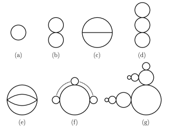
Figure 2: Examples of the various types of 1PI diagrams which contribute to the effective potential for a $\lambda\phi^{4}$ theory. In particular, diagrams of the type (f), are called “daisies” and those of type (g), super–daisies, or foam diagrams respectively.

I.3.2 The Cornwall–Jackiw–Tomboulis method

Another way to perform systematic selective summations is to use the method of the effective action for composite operators Cornwall:1974vz . In this case, the effective action is the generating functional of the two–particle irreducible (2PI) vacuum graphs (a graph is called “two–particle irreducible” if it does not become disconnected upon opening two lines). Now, the effective action $\Gamma(\phi,G)$, depends not only on $\phi(x)$, but on $G(x,y)$, as well. These two quantities are to be realized as the possible expectation values of a quantum field $\Phi(x)$ and as the time ordered product of the field operator $T\Phi(x)\Phi(y)$ respectively. This formalism was initially used for a study of the $O(N)$ model at zero temperature Cornwall:1974vz , but it has been extended to finite–temperature by Amelino–Camelia and Pi, and was used for investigations of the effective potential of the $\lambda\phi^{4}$ theory Amelino-Camelia:1993nc , and gauge theories Amelino-Camelia:1994kd .

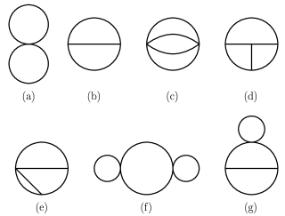
Figure 3: a–e: Examples of two–particle irreducible graphs which contribute to the effective potential in the CJT method, up to three loops. The lines represent “dressed” propagators $G(x,y)$. f–g: These graphs are two–particle reducible. They do not contribute in the CJT method, however they do contribute to ordinary effective action $\Gamma(\phi)$. In this case the lines represent the tree–level propagator $D(\phi;x,y)$.

There is an advantage in using the CJT method to calculate the effective potential in certain approximations as is, for example, the Hartree approximation of the $\lambda\phi^{4}$ theory. According to reference Amelino-Camelia:1993nc , if we use an ansatz for a “dressed propagator”, we need to evaluate only one graph, that of the “double bubble” in Fig. 3a, instead of summing the infinite class of “daisy” and “super–daisy” graphs, given in Figs.2f,g, using the usual tree level propagators.

We demonstrate the advantage of this method in Section I.5, where we calculate the finite–temperature effective potential for one scalar field, with quartic self–interaction. The calculation of the effective potential by using the CJT formalism is reviewed, in detail, in references Amelino-Camelia:1993nc ; Amelino-Camelia:1996hw , but in order to illustrate the method for the calculation of the effective potential for the linear sigma model at finite–temperature, we will reproduce the basic steps here. For this presentation we follow closely the derivation as in Cornwall:1974vz .

In order to define the effective action for composite operators, we can follow a path analogous to the one leading to the ordinary effective action. The essential difference is that the partition function depends also on a bilocal source $K(x,y)$, in addition to the local source $J(x)$. As an example, we consider the $\lambda\Phi^{4}$ theory with Lagrangian

$$\mathcal{L}(\Phi)=\frac{1}{2}\,\partial_{\mu}\Phi\,\partial^{\mu}\Phi-\frac{1}{2}\,m^{2}\Phi^{2}-\frac{\lambda}{24}\,\Phi^{4}~{}.$$ (27)

According to CJT method Cornwall:1974vz , the generating functional for the Green functions in the presence of sources $J(x)$ and $K(x,y)$ is given by (we set $\hbar=1$)

$$\mathcal{Z}(J,K)=e^{\mathcal{W}(J,K)}=\int\mathcal{D}\Phi\exp\bigg{[}I(\Phi)+\Phi J+\frac{1}{2}\Phi K\Phi\bigg{]}$$ (28)

where $\mathcal{W}(J,K)$, is the generating functional for the connected Green functions, while $I(\Phi)=\int dx^{4}\,\mathcal{L}(x)$ is the classical action. Adopting a similar notation as Rischke and Lenaghan Lenaghan:2000si , we have used the shorthands

$$\Phi\,J \equiv \int d^{4}x\,\Phi(x)\,J(x)~{},$$ (29)

$$\Phi\,K\,\Phi \equiv \int d^{4}xd^{4}y\,\Phi(x)\,K(x,y)\,\Phi(y)~{}.$$ (30)

The expectation values for the one–point function, $\phi(x)$, in the presence of a source $J(x)$ is given by

$$\frac{\delta\mathcal{W}(J,K)}{\delta J(x)}\equiv\phi(x)~{},$$ (31)

while the connected two–point function, $G(x,y)$ is

$$\frac{\delta\mathcal{W}(J,K)}{\delta K(x,y)}\equiv\frac{1}{2}\big{[}G(x,y)+\phi(x)\,\phi(y)\big{]}~{}.$$ (32)

The effective action for composite operators $\Gamma(\phi,G)$, is obtained through a double Legendre transformation of $\mathcal{W}(J,K)\equiv\ln\mathcal{Z}(J,K)$

$$\Gamma(\phi,G)=\mathcal{W}(J,K)-\phi\,J-\frac{1}{2}\,\phi\,K\,\phi-\frac{1}{2}\,G\,K~{},$$ (33)

where $G\,K=\int d^{4}xd^{4}y\,G(x,y)\,K(y,x)$. Then it follows that

$$\frac{\delta\Gamma(\phi,G)}{\delta\phi(x)} = -J(x)-\int d^{4}y\,K(x,y)\,\phi(y)~{},$$ (34)

$$\frac{\delta\Gamma(\phi,G)}{\delta G(x,y)} = -\frac{1}{2}\,K(x,y)~{}.$$ (35)

Physical processes correspond to vanishing sources, so the stationarity conditions which determine the expectation value of the field $\varphi(x)$, and the (dressed) propagator $\mathcal{G}(x,y)$ are given by

$$\frac{\delta\Gamma(\phi,G)}{\delta\phi(x)}\,\bigg{|}_{\phi=\varphi,\,G=\mathcal{G}} = 0~{},$$ (36)

$$\frac{\delta\Gamma(\phi,G)}{\delta G(x,y)}\bigg{|}_{\phi=\varphi,\,G=\mathcal{G}} = 0~{}.$$ (37)

As it was shown by Cornwall–Jackiw–Tomboulis in Cornwall:1974vz , the effective action $\Gamma(\phi,G)$ is given by

$$\Gamma(\phi,G) = I(\phi)-\frac{1}{2}\textrm{Tr}\left(\ln\,G^{-1}\right)$$

$$-\frac{1}{2}\textrm{Tr}\left(D^{-1}\,G-1\right)+\Gamma_{2}(\phi,G)~{},$$

where in this last equation $\Gamma_{2}(\phi,G)$ is the sum of all two particle irreducible (2PI) diagrams in which all lines represent full (dressed) propagators $G$, while $D^{-1}$ is the inverse of the tree–level propagator,

$$D^{-1}(x,y;\phi)\equiv-\frac{\delta^{2}I(\phi)}{\delta\phi(x)\,\delta\phi(y)}\bigg{|}_{\phi=\varphi}~{}.$$ (39)

In the case when translation invariance is not broken, it can be assumed that the field $\phi(x)=\textrm{constant}=\phi$. Then an infinite volume factor $\Omega$ arises from space–time integrations and it is customary to introduce the generalized effective potential $V(\phi,G)=\Gamma(\phi,G)/\Omega$. The exact expression for the effective potential is then

$$V(\phi,G) = U(\phi)+\frac{1}{2}\int_{k}\,\ln G^{-1}(k)$$

$$+\frac{1}{2}\,\int_{k}\,\big{[}D^{-1}(k;\phi)\,G(k)-1\big{]}+V_{2}(\phi,G)~{},$$

where is $U(\phi)$ is the classical potential of the Lagrangian, $D^{-1}(k;\phi)$ is the inverse tree level propagator, which for $\lambda\phi^{4}$ theory is given by

$$D^{-1}(k;\phi)=k^{2}+m^{2}+\frac{1}{2}\lambda\phi^{2}~{},$$ (41)

and $V_{2}(\phi,G)=\Gamma_{2}(\phi,G)/\Omega$. The stationarity conditions for the effective action reduce to the following ones involving the effective potential

$$\frac{\delta V(\phi,G)}{\delta\phi}\,\bigg{|}_{\phi=\varphi,\,G=\mathcal{G}}=0~{},$$ (42)

$$\frac{\delta V(\phi,G)}{\delta G(k)}\,\bigg{|}_{\phi=\varphi,\,G=\mathcal{G}}=0~{}.$$ (43)

We then obtain the following relation

$$\mathcal{G}^{-1}(k)=D^{-1}(k;\varphi)+\Sigma(k)~{},$$ (44)

which corresponds to a Schwinger–Dyson equation for the full (dressed) propagator $\mathcal{G}$ and where the self–energy $\Sigma(k)$ is given by

$$\Sigma(k)\equiv 2\frac{\delta V_{2}(\phi,G)}{\delta G(k)}\bigg{|}_{\phi=\varphi,\,G=\mathcal{G}}~{}.$$ (45)

The thermal effective potential has the meaning of the free energy density and it is related to thermodynamic pressure through the equation

$$p=-V(\varphi,\mathcal{G})~{}.$$ (46)

I.4 Finite temperature formalisms

Whatever the method one chooses to calculate the effective potential, the calculation has to be performed in the framework of finite temperature field theory. There are three main paths to follow namely: thermo–field dynamics, imaginary time formalism and real time formalism. In our calculations, we do not use the machinery of thermo–field dynamics, but we use both real and imaginary time. Each of these has certain advantages and disadvantages. Traditionally, the imaginary time seems to be convenient for systems in equilibrium, since the real time is thought to be the appropriate for calculations in systems far from equilibrium.

I.4.1 Imaginary time formalism

The imaginary time formalism, which is also known as the Matsubara formalism, provides a way of evaluating the partition function perturbatively using a diagrammatic method which is analogous to that which is used in conventional field theory at zero temperature Dolan:1974qd ; Kapusta:1989 ; Das:1997gg ; Landsman:1987uw . According to this technique, we work in Euclidean space–time and use the same Feynman rules as at zero–temperature, but when evaluating momentum space integrals, we replace integration over the time component $k_{4}$ with a summation over discrete frequencies. That means that in the case of bosons $k_{4}=2\pi inT,\;\;n=0,\pm 1,\pm 2,\pm 3,\ldots$. This is encoded into the following relationship

$$\int\frac{d^{4}k}{(2\pi)^{4}}f(k)\longrightarrow\frac{1}{\beta}\sum_{n}\int\frac{d^{3}\textbf{k}}{(2\pi)^{3}}f(2\pi inT,\textbf{k})$$ (47)

where $\beta$ is the inverse temperature, $\beta=1/k_{B}T$, and as usual Boltzmann’s constant is taken to be $k_{B}=1$. For the sake of simplicity, in the following we introduc a subscript $\beta$, to denote integration and summation over the Matsubara frequency sums. So in what follows we adopt the shorthand expression

$$\frac{1}{\beta}\sum_{n}\int\frac{d^{3}\textbf{k}}{(2\pi)^{3}}f(2\pi inT,\textbf{k})\equiv\int_{\beta}f(2\pi inT,\textbf{k})~{}$$ (48)

If one is to study systems at equilibrium, the imaginary time formalism is adequate, but for dynamical systems far from equilibrium, we need to analytically continue back to real time which was traded in favour of the temperature. An alternative way is to work directly in the real time formalism from the outset. We introduce the basic concepts about the real time formalism in the next section.

I.4.2 Real time formalism

This formalism has a long history of applications in condensed matter systems, where early papers appeared in the 1950’s. It is also known as Keldysh or closed–path formalism Keldysh:ud . It has only been quite recently that researchers realized its usefulness in applications in particle physics at finite–temperature. The formalism is given in details in Niemi:1984nf ; Niemi:1984ea , and is also reviewed in Landsman:1987uw , where a formal account for both – real time and imaginary time – formalisms is given. There is also a lot of information in the recent books Rivers:1987 ; LeBellac:1996 ; Das:1997gg . Further information can also be found in recent papers Das:2000ft ; Landshoff:1998ku ; Altherr:1993tn .

The basic point is that for a scalar field theory, the propagator becomes a two by two matrix and is divided into two parts as

$$i\mathcal{D}=i\mathcal{D}_{0}+i\mathcal{D_{\beta}}~{},$$ (49)

where the zero temperature part appears as

$$i\mathcal{D}_{0}=\begin{bmatrix}\displaystyle\frac{i}{k^{2}-m^{2}+i\epsilon}&0\\ 0&\displaystyle\frac{-i}{k^{2}-m^{2}-i\epsilon}\\ \end{bmatrix}$$ (50)

and the temperature dependent part is of the form

$$i\mathcal{D_{\beta}}=\frac{\epsilon}{(k^{2}-m^{2})^{2}+\epsilon^{2}}\begin{bmatrix}2\sinh^{2}\theta&\sinh\;2\theta\\ \sinh\;2\theta&2\sinh^{2}\theta\\ \end{bmatrix}~{},$$ (51)

where

$$\cosh^{2}\theta=\frac{{\rm e}^{\beta|k_{0}|}}{{\rm e}^{\beta|k_{0}|}-1}~{}.$$ (52)

In the limit $\epsilon\rightarrow 0$, the pre–factor of the thermal part reduces to a delta function.

In particular the $(1,1)$ component is given by

$$\mathcal{D}^{11}=\frac{i}{k^{2}-m^{2}+i\epsilon}+2\pi\delta(k^{2}-m^{2})n(k_{0})$$ (53)

where $n(k_{0})$ is the Bose–Einstein distribution function

$$n(k_{0})=\frac{1}{\exp(\beta|k_{0}|)-1}~{}.$$ (54)

In this last equation $\beta=1/T$ is the inverse temperature, while $k_{0}=\sqrt{\textbf{k}^{2}+m^{2}}$.

I.5 The $\lambda\Phi^{4}$ theory at finite temperature

As an illustration, we use the CJT formalism to calculate the effective potential for a $\lambda\Phi^{4}$ theory. The Lagrangian is given by

$$\mathcal{L}=\frac{1}{2}(\partial_{\mu}\Phi)(\partial^{\mu}\Phi)-\frac{1}{2}m^{2}\Phi^{2}-\frac{1}{24}\lambda\Phi^{4}~{},$$ (55)

and in order to realize the spontaneous breaking of symmetry, $m^{2}$ is considered as a negative parameter. By shifting the field as $\Phi\rightarrow\Phi+\phi$, the “classical potential” takes the form

$$U(\phi)=\frac{1}{2}m^{2}\phi^{2}+\frac{1}{24}\lambda\phi^{4}~{},$$ (56)

and the interaction Lagrangian which describes the vertices of the shifted, theory is given by

$$\mathcal{L}_{int}=-\frac{\lambda}{6}\phi\Phi^{3}-\frac{\lambda}{24}\Phi^{4}~{}.$$ (57)

The tree–level propagator which corresponds to the above Lagrangian density is

$$\mathcal{D}^{-1}(\phi;k)=k^{2}+m^{2}+\frac{1}{2}\lambda\phi^{2}~{}.$$ (58)

According to CJT formalism Amelino-Camelia:1993nc , the finite temperature effective potential is given by

$$V(\phi,G) = U(\phi)+\frac{1}{2}\int_{\beta}\ln G^{-1}(\phi;k)$$ (59)

$$+\frac{1}{2}\int_{\beta}[\mathcal{D}^{-1}(\phi;k)G(\phi;k)-1]$$

$$+V_{2}(\phi,G)~{},$$

where $U(\phi)$ is the “classical potential” given by Eq. (56), and $V_{2}(\phi,G)$ represents the infinite sum of the two–particle irreducible vacuum graphs. We are going to evaluate the effective potential in the Hartree approximation which means that we only need to calculate the “double bubble” diagram given in Fig. 3 (a). The resulting effective potential, is therefore,

$$V(\phi,G) = \frac{1}{2}m^{2}\phi^{2}+\frac{1}{24}\lambda\phi^{4}+\frac{1}{2}\int_{\beta}\ln G^{-1}(\phi;k)$$ (60)

$$+\frac{1}{2}\int_{\beta}[(k^{2}+m^{2}+\frac{1}{2}\lambda\phi^{2})G(\phi;k)-1]$$

$$+\frac{1}{8}\lambda\big{[}\int_{\beta}G(\phi;k)\big{]}^{2}~{}.$$

Minimizing the effective potential with respect to the “dressed propagator” $G(\phi;k)$, we obtain the gap equation

$$G^{-1}(\phi;k)=k^{2}+m^{2}+\frac{1}{2}\lambda\phi^{2}+\frac{1}{2}\lambda\int_{\beta}G(\phi;k)~{}.$$ (61)

In graphical terms, we could say that the self–energy is calculated by opening one line of each diagram contained in the functional of the effective potential vanHees:2000bp ; Ivanov:2000ma . In Hartree approximation, this is illustrated in the Fig. 4 .

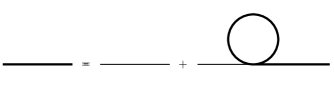
Figure 4: Schematic representation of the self–energy contribution to scalar propagator in the self–consistent Hartree approximation. The full or “dressed” propagator appears as a sum of the bare propagator, and the self–energy insertion.

The solution $G_{0}(\phi;k)$, of the gap equation, is inserted back into the expression for the effective potential, resulting in a potential which is a function of $\phi$. As is stated in Cornwall:1974vz , using the propagator $G_{0}(\phi;k)$ for internal lines corresponds to summing all daisy and super-daisy diagrams, using the usual tree level propagators as in Dolan:1974qd .

Then, we can adopt the following form for the dressed propagator $G(\phi;k)$,

$$G(\phi;k)=\frac{1}{k^{2}+M^{2}}~{},$$ (62)

where an “effective mass” $M=M(\phi;k)$, has been introduced. The gap equation for the propagator then becomes an equation for the effective mass

$$M^{2}=m^{2}+\frac{\lambda}{2}\phi^{2}+\frac{\lambda}{2}\int_{\beta}\frac{1}{k^{2}+M^{2}}~{},$$ (63)

where it is obvious, since we integrate over the loop momenta, that in this approximation, the effective mass $M$ is momentum independent.

In terms of the solution $M_{0}(\phi)$ of the gap Eq. (63), the effective potential takes the form

$$V(\phi,M_{0}) = \frac{1}{2}m^{2}\phi^{2}+\frac{\lambda}{24}\phi^{4}+\frac{1}{2}\int_{\beta}\ln(k^{2}+M^{2}_{0})$$ (64)

$$-\frac{1}{2}(M^{2}_{0}-m^{2}-\frac{\lambda}{2}\phi^{2})\int_{\beta}\frac{1}{k^{2}+M^{2}_{0}}$$

$$+\frac{\lambda}{8}\big{[}\int_{\beta}\frac{1}{k^{2}+M_{0}^{2}}\big{]}^{2}~{}.$$

Performing the Matsubara frequency sums as in Dolan:1974qd (we repeat these steps in appendix A), the logarithmic integral which appears in the above expression for the effective potential divides into two parts. A zero–temperature part, $Q_{0}(M)$, which is divergent, and a nonzero–temperature part, $Q_{\beta}(M)$, which is finite, and can be written as

$$Q(M) = \frac{1}{2}\int_{\beta}\ln(k^{2}+M^{2})$$ (65)

$$= Q_{0}(M)+Q_{\beta}(M)$$

$$= \int\frac{d^{3}\textbf{k}}{(2\pi)^{3}}\frac{\omega_{\textbf{k}}}{2}$$

$$+\frac{1}{\beta}\int\frac{d^{3}\textbf{k}}{(2\pi)^{3}}\ln[1-\exp(-\beta\omega_{\textbf{k}})]~{},$$

where $\omega_{\textbf{k}}=(\textbf{k}^{2}+M^{2})^{1/2}$. In this above expression, and in what follows, we omit the subscript 0 on $M$. Similarly, the second integral is divided into a zero–temperature part $F_{0}(M)$, and a finite–temperature part $F_{\beta}(M)$, given by

$$F(M) = \int_{\beta}\frac{1}{k^{2}+M^{2}}$$ (66)

$$= F_{0}(M)+F_{\beta}(M)$$

$$= \int\frac{d^{3}\textbf{k}}{(2\pi)^{3}}\frac{1}{2\omega_{\textbf{k}}}$$

$$+\int\frac{d^{3}\textbf{k}}{(2\pi)^{3}}\frac{1}{\omega_{\textbf{k}}}\frac{1}{\exp(\beta\omega_{\textbf{k}})-1}~{}.$$

The second term vanishes at zero temperature, while the first term survives but it gives rise to divergences which can be carried out using appropriate renormalization prescriptions Amelino-Camelia:1993nc ; Amelino-Camelia:1996hw . If one is interested in temperature induced effects only, as is our approximation, the divergent integrals can be ignored. In this case, by making a change to the integration variables, the finite–temperature part of $F(M)$ can be written as

$$F_{\beta}(M)=\frac{T^{2}}{2\pi^{2}}\int_{0}^{\infty}\frac{x^{2}\,dx}{(x^{2}+y^{2})^{1/2}}\frac{1}{\exp(x^{2}+y^{2})^{1/2}-1}~{},$$ (67)

where we have used a shorthand notation, $y=M/T$.

In order to simplify the lengthy expressions involved in what follows, we introduce the function $g(z,a)$ defined as

$$g(z,a)=\frac{1}{(z^{2}+a^{2})^{1/2}}\frac{1}{\exp(z^{2}+a^{2})^{1/2}-1}~{}.$$ (68)

Then the function $f(a)$, will appear as the shorthand of the integral

$$f(a) = \int_{0}^{\infty}\frac{x^{2}dx}{(x^{2}+a^{2})^{1/2}}\frac{1}{\exp(x^{2}+a^{2})^{1/2}-1}$$

$$= \int_{0}^{\infty}x^{2}\,dx\,g(x,a)~{},$$

and in the limit of $a=0$, we recover the well known result $f(0)=\pi^{2}/6$.

Similarly, the finite–temperature part of the logarithmic integral becomes

$$Q_{\beta}(M)=\frac{T^{4}}{2\pi^{2}}\int_{0}^{\infty}x^{2}\,dx\ln\left(1-\exp[-(x^{2}+y^{2})^{1/2}]\right)~{}.$$ (70)

Then, the finite–temperature effective potential, ignoring quantum fluctuations, can be written as

$$V(\phi,M) = \frac{1}{2}m^{2}\phi^{2}+\frac{1}{24}\lambda\phi^{4}+Q_{\beta}(M)$$ (71)

$$\mbox{}-\frac{1}{2}(M^{2}-m^{2}-\frac{\lambda}{2}\phi^{2})F_{\beta}(M)$$

$$+\frac{\lambda}{8}[F_{\beta}(M)]^{2}~{}.$$

We can obtain a more compact form if we make use of the gap equation (63),

$$V(\phi,M)=\frac{1}{2}m^{2}\phi^{2}+\frac{1}{24}\lambda\phi^{4}+Q_{\beta}(M)-\frac{1}{8}\lambda\big{[}F_{\beta}(M)\big{]}^{2}~{}.$$ (72)

II Hartree approximation

II.1 Introduction

In this section, we apply the CJT method in order to calculate the effective potential of the $O(4)$ linear sigma model. The $\sigma$ field can be used to represent the quark condensate, the order parameter for the chiral phase transition, since both exhibit the same behaviour under chiral transformations Birse:1994cz ; Hatsuda:2000by ; Kunihiro:2000je . The pions are very light particles, and can be considered approximately as massless Goldstone bosons. We use the model as an effective theory for QCD, ignoring the fermion sector for the moment, and concentrating on the meson sector. We examine this model in two approximation schemes: (a) in the chiral limit considering the pions true Goldstone bosons, and therefore massless, and (b) treating them as massive.

II.2 The linear sigma model

As we mentioned in the introduction, the linear sigma model serves as a good low energy effective theory in order for one to gain some insight into QCD. Recently, it has attracted much attention, especially in studies involving disoriented chiral condensates (DCC’s) Bjorken:1992xr ; Abada:1998mb ; Randrup:1997es ; Randrup:1996ay ; Rajagopal:1993ah . The model is very well suited for describing the physics of pions in studies of chiral symmetry. Fermions may be included in the model either as nucleons, if one is to study nucleon interactions, or as quarks. The mesonic part of the model consists of four scalar fields, one scalar isoscalar field which is called the sigma $\sigma$ field and the usual three pion fields $\pi^{0}$, $\pi^{\pm}$, which form a pseudo–scalar isovector. The fields form a four vector $(\sigma,\pi_{i}),\;\;i=1,2,3$, which we regard as the chiral field and the model displays an $O(4)$ symmetry.

The meson sector Lagrangian of the $O(4)$ sigma model is

$$\mathcal{L} = \frac{1}{2}(\partial\sigma)^{2}+\frac{1}{2}(\partial\bm{\pi})^{2}-\frac{1}{2}m^{2}\sigma^{2}-\frac{1}{2}m^{2}\bm{\pi}^{2}$$ (73)

$$-\frac{\lambda}{24}(\sigma^{2}+\bm{\pi}^{2})^{2}-\varepsilon\sigma~{}.$$

The last term, $\varepsilon\sigma$, has been introduced into the above expression in order to generate masses for the pions. It is related to pion mass as $\varepsilon=f_{\pi}m_{\pi}^{2}$, where $f_{\pi}=93\,\,\rm MeV$, is the pion decay constant. In the absence of the last term which breaks the chiral symmetry, the pions are massless.

The coupling constant $\lambda$ of the model can be related to zero temperature properties of the pions, and sigma through the expression

$$\lambda=\frac{3(m_{\sigma}^{2}-m_{\pi}^{2})}{f_{\pi}^{2}}~{}.$$ (74)

The negative mass parameter $m^{2}$, is introduced in order to obtain spontaneous breaking of symmetry and its value is chosen to be

$$-m^{2}=(m_{\sigma}^{2}-3m_{\pi}^{2})/2>0~{}.$$ (75)

To define the numerical values of $\lambda$ and $m^{2}$, we use $m_{\pi}\approx 138\,\textrm{MeV}$, since for the sigma mass we adopt $m_{\sigma}\approx 600\,\textrm{MeV}$.

II.3 The chiral limit $\varepsilon=0$

In order to deal with the exact chiral limit first, the starting point is the Lagrangian given in Eq. (73), and we ignore the symmetry breaking term for the moment. The parameters $\lambda$ and $m^{2}$ appearing in the Lagrangian are simply

$$\lambda=\frac{3m_{\sigma}^{2}}{f_{\pi}^{2}},\qquad-2m^{2}=m_{\sigma}^{2}>0~{}.$$ (76)

By shifting the sigma field as $\sigma\rightarrow\sigma+\phi$, the resulting “classical potential” is

$$U(\phi)=\frac{1}{2}m^{2}\phi^{2}+\frac{\lambda}{24}\phi^{4}~{},$$ (77)

and the interaction Lagrangian which describes the vertices of the new theory takes the form

$$\mathcal{L}_{int}=-\frac{\lambda}{24}\sigma^{4}-\frac{\lambda}{24}{\bm{\pi}}^{4}-\frac{\lambda}{12}\sigma^{2}{\bm{\pi}}^{2}-\frac{\lambda}{6}\phi\sigma^{3}-\frac{\lambda}{6}\phi\sigma{\bm{\pi}}^{2}~{}.$$ (78)

In the Hartree approximation, we do not consider interactions given by the last two terms in the Lagrangian. We attempt to include these interactions in Section IV.

The tree level sigma, and pion propagators, corresponding to the above Lagrangian are

$$\mathcal{D}^{-1}_{\sigma}(\phi;k) = k^{2}+m^{2}+\frac{1}{2}\lambda\phi^{2}~{},$$ (79)

$$\mathcal{D}^{-1}_{\pi}(\phi;k) = k^{2}+m^{2}+\frac{1}{6}\lambda\phi^{2}~{}.$$ (80)

We evaluate the effective potential in the Hartree approximation, which means that we only need to calculate the “double bubble” diagrams as in $\lambda\phi^{4}$ theory. In the linear sigma model, the corresponding effective potential at finite temperature can be written as

$$V(\phi,G) = U(\phi)+\frac{1}{2}\int_{\beta}\ln G^{-1}_{\sigma}(\phi;k)+\frac{3}{2}\int_{\beta}\ln G^{-1}_{\pi}(\phi;k)$$ (81)

$$+\frac{1}{2}\int_{\beta}[\mathcal{D}_{\sigma}^{-1}(\phi;k)G_{\sigma}(\phi;k)-1]$$

$$+\frac{3}{2}\int_{\beta}[\mathcal{D}_{\pi}^{-1}(\phi;k)G_{\pi}(\phi;k)-3]$$

$$+V_{2}(\phi,G_{\sigma},G_{\pi})~{},$$

where the first term $U(\phi)$, is the classical potential and the last term $V_{2}(\phi,G_{\sigma},G_{\pi})$, originates from the sum of “double bubble” diagrams. There are four types of double bubbles as we show in Fig. 5, and these contribute the following terms in the potential

$$V_{2}(\phi,G_{\sigma},G_{\pi}) = 3\frac{\lambda}{24}\left[\int_{\beta}G_{\sigma}(\phi;k)\right]^{2}$$ (82)

$$+6\frac{\lambda}{24}\int_{\beta}G_{\sigma}(\phi;k)\int_{\beta}G_{\pi}(\phi;k)$$

$$+15\frac{\lambda}{24}\left[\int_{\beta}G_{\pi}(\phi;k)\right]^{2}~{}.$$

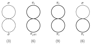
Figure 5: Graphs of the “double–bubble” type which contribute to the effective potential for the O(4) linear sigma model in the Hartree approximation. The numbers show the weight of each type of bubble, in the expression for the effective potential.

Minimizing the effective potential with respect to the “dressed” propagators, we get the following pair of nonlinear gap equations

$$G_{\sigma}^{-1}(\phi;k) = \mathcal{D}_{\sigma}^{-1}+\frac{\lambda}{2}\int_{\beta}G_{\pi}(\phi;k)+\frac{\lambda}{2}\int_{\beta}G_{\sigma}(\phi;k)~{},$$

$$G_{\pi}^{-1}(\phi;k) = \mathcal{D}_{\pi}^{-1}+\frac{5\lambda}{6}\int_{\beta}G_{\pi}(\phi;k)+\frac{\lambda}{6}\int_{\beta}G_{\sigma}(\phi;k)~{}.$$

The bare propagators $\mathcal{D}_{\sigma}$ and $\mathcal{D}_{\pi}$ are given by Eq. (79). In order to solve this system, we can use the same ansatz for the dressed propagators as in the one field case

$$G_{\sigma/\pi}^{-1}=k^{2}+M^{2}_{\sigma/\pi}~{}.$$ (83)

Then by using Eqs. (79), (LABEL:Eq:gap-prop) the nonlinear system for the dressed propagators reduces to the following system for the thermal effective masses

$$M_{\sigma}^{2} = m^{2}+\frac{1}{2}\lambda\phi^{2}+\frac{\lambda}{2}F(M_{\sigma})+\frac{\lambda}{2}F(M_{\pi})$$ (84a)

$$M_{\pi}^{2} = m^{2}+\frac{1}{6}\lambda\phi^{2}+\frac{\lambda}{6}F(M_{\sigma})+\frac{5\lambda}{6}F(M_{\pi})~{}.$$ (84b)

In these last two equations, we have used a shorthand notation and $F(M_{\sigma/\pi})$ is given by

$$F(M_{\sigma/\pi})=\int_{\beta}\frac{1}{k^{2}+M^{2}_{\sigma/\pi}}~{}.$$ (85)

As in $\lambda\phi^{4}$ theory, the thermal effective masses are independent of momentum and functions of the order parameter $\phi$, and the temperature $T$.

By using these two equations, the effective potential at finite temperature can be written as

$$V(\phi,M) = \frac{1}{2}m^{2}\phi^{2}+\frac{1}{24}\lambda\phi^{4}$$ (86)

$$+\frac{1}{2}\int_{\beta}\ln(k^{2}+M_{\sigma}^{2})+\frac{3}{2}\int_{\beta}\ln(k^{2}+M_{\pi}^{2})$$

$$-\frac{1}{2}(M_{\sigma}^{2}-m^{2}-\frac{1}{2}\lambda\phi^{2})F(M_{\sigma})$$

$$-\frac{3}{2}(M_{\pi}^{2}-m^{2}-\frac{1}{6}\lambda\phi^{2})F(M_{\pi})$$

$$+\frac{\lambda}{8}[F(M_{\sigma})]^{2}+\frac{5\lambda}{8}[F(M_{\pi})]^{2}$$

$$+\frac{\lambda}{4}F(M_{\sigma})F(M_{\pi})~{}.$$

Minimizing the effective potential with respect to the “dressed” propagators, we have found the set of nonlinear gap equations for the effective particles’ masses, given by Eq. (84). In addition, by minimizing the potential with respect to the order parameter, we obtain one more equation

$$0=m^{2}+\frac{1}{6}\lambda\phi^{2}+\frac{\lambda}{2}F(M_{\sigma})+\frac{\lambda}{2}F(M_{\pi})~{}.$$ (87)

In order to study the evolution of the potential as a function of temperature, we perform the Matsubara frequency sums, as in the one field case. There are some problems concerning the renormalization of the model Amelino-Camelia:1993nc ; Amelino-Camelia:1997dd ; Baym:1977qb ; Roh:1998ek . At the level of our approximation, we ignore quantum fluctuations for the moment, and keep only the finite temperature part of the integrals. This decision is justified by the fact that the finite terms – given by Eq. (67) and Eq. (70) – correspond to interactions between thermallly excited mesons with other mesons present in the plasma Rivers:1994rz . In doing so, we neglect the quantum fluctuations of the meson fields and keep only the thermal fluctuations present in the hot plasma. The same choice was also adopted in Roh:1998ek ; Larsen:1986ei . In a very recent investigation of the same model, and based on the same formalism, Rischke and Lenaghan Lenaghan:2000si have shown that the model is indeed renormalisable. Renormalization of the model has also demonstrated by Chiku and Hatsuda Chiku:1998va ; Chiku:1998kd , who on the basis of optimised perturbation theory, and the real time formalism, have studied the spectral densities and the effective masses of the sigma and the pions.

Diagrammatically, differentiation of the double bubbles in Fig. 5 gives the selfenergy loop contribution to the particle propagators as we show in Figs. 6,7. We can picture the dressed propagator with a thick line which appears as a sum of the bare propagator (not shown in the figures) and the selfenergy contributions. Actually one can see these two figures as a graphical representation of the gap equations for the dressed propagators. As we have mentioned already, at finite temperature and in the real time formalism, the propagators appear to consist of two parts, a zero temperature part and a thermal part. We denote each zero tempearture loop with continuous line and each thermal with a cut. Our choice to keep only the non divergent parts of the integrals, is equivalent to taking into account only the thermal propagators. This means that for pions, we are taking into account only the thermal self energy loops in Figs. 6b, d while for sigma those in Figs. 7b,d.

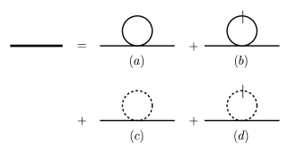
Figure 6: Schematic presentation of selfenergy contribution to pion propagator. Dashed lines represent sigma propagator, while continuous ones correspond to pions.

Figure 7: Schematic presentation of selfenergy contribution to sigma propagator. Dashed lines represent sigma propagator, while continuous ones correspond to pions.

Using a compact notation, the finite temperature effective potential can be written in the form

$$V(\phi,M) = \frac{1}{2}m^{2}\phi^{2}+\frac{1}{24}\lambda\phi^{4}$$ (88)

$$+Q_{\beta}(M_{\sigma})+3Q_{\beta}(M_{\pi})$$

$$-\frac{\lambda}{8}[F_{\beta}(M_{\sigma})]^{2}-\frac{5\lambda}{8}[F_{\beta}(M_{\pi})]^{2}$$

$$-\frac{\lambda}{4}F_{\beta}(M_{\sigma})F_{\beta}(M_{\pi})~{},$$

where in this last step, we have used the gap equations given by Eq. (84). The exact expressions for $F_{\beta}(M)$ and $Q_{\beta}(M)$, are given by Eq. (67) and Eq. (70) respectively.

II.3.1 High temperature limit

In order to calculate the effective masses as functions of temperature, we need to solve the system of the three equations given by Eq. (84) and Eq. (87). We first observe that if $\phi=0$, which happens in the high temperature phase, the two equations become degenerate, the particles have the same mass, and we have to solve only one equation

$$M^{2}=m^{2}+\lambda F_{\beta}(M)~{}.$$ (89)

As in the expression of the effective potential, we keep only the finite temperature part of the integral. This last equation can be used to define a “transition temperature” $T_{c1}$. This temperature is defined as the temperature, where both particles become massless. Recall now that $F_{\beta}(M)$ is given by

$$F_{\beta}(M)=\frac{T^{2}}{2\pi^{2}}\int_{0}^{\infty}\frac{x^{2}\,dx}{a^{1/2}}\frac{1}{\exp(a^{1/2})-1}~{},$$ (90)

where $a=x^{2}+y^{2}$ and $y=M/T$. When the mass of the particles vanishes, this integral reduces to the well known result

$$I(x)=\int_{0}^{\infty}\frac{x\,dx}{e^{x}-1}=\frac{\pi^{2}}{6}~{}.$$ (91)

Therefore by using Eqs. (89), (90) and (91), we find that

$$0=m^{2}+\lambda\,\frac{T^{2}}{2\pi^{2}}\,\frac{\pi^{2}}{6}~{}.$$ (92)

Actually this defines the transition temperature $T=T_{c1}$ as

$$T_{c1}=\sqrt{2}\bigg{(}-\frac{6m^{2}}{\lambda}\bigg{)}^{1/2}~{}.$$ (93)

But, in defining our model parameters, we have chosen that at zero temperature $\phi^{2}=f_{\pi}^{2}=-6m^{2}/\lambda$, where $f_{\pi}=93\;\rm MeV$ is the pion decay constant, so we find that $T_{c1}=\sqrt{2}f_{\pi}\approx 131.5\;\rm MeV$.

II.3.2 Low temperature limit

In the low temperature phase, we can eliminate $\phi$ between Eqs. (84) and (87). We then end up with the following nonlinear system

$$M_{\sigma}^{2} = -2m^{2}-\lambda F_{\beta}(M_{\sigma})-\lambda F_{\beta}(M_{\pi})$$

$$M_{\pi}^{2} = -\frac{\lambda}{3}F_{\beta}(M_{\sigma})+\frac{\lambda}{3}F_{\beta}(M_{\pi})~{}.$$ (94)

where, as before, we have ignored the divergent parts of $F(M_{\sigma/\pi})$. This system has been solved numerically using a Newton–Raphson method, and the solution is presented in Fig. 8 .

Figure 8: Solution of the system of gap equations in the chiral limit, $\varepsilon=0$. The sigma and pion effective masses are given as functions of temperature.

As shown in Fig. 8, the temperature $T_{c1}$ which is calculated numerically, was found to be in excellent agreement with the value obtained by using the limit of the high temperature equations with degenerate masses.

At this point, we can observe that there is an indication of a first order phase transition, because combining Eq. (84b) with Eq. (87), we find that

$$M_{\sigma}^{2}=\frac{1}{3}\lambda\phi^{2}~{}.$$ (95)

This last equation shows, of course, that the order parameter varies with temperature proportionally to the sigma mass. The temperature dependence of $\phi=\phi(T)$, is calculated by using the sigma mass as it was found by solving the system in Eq. (94). This is shown in Fig. 9, where it is obvious that this approximation predicts a first order phase transition, because $\phi$, which is the order parameter of the phase transition, appears to have two different values for the same temperature.

Figure 9: Evolution of the order parameter $\phi$ as a function of temperature.

This last observation coincides with the qualitative picture given by Baym and Grinstein, in their early paper Baym:1977qb , where their “modified Hartree approximation” predicts a first order phase transition, as well. However, in contrast to our approximation, they had included quantum fluctuations into their analysis as well. Signals of a first order phase transition have also been reported in recent analyses by Randrup Randrup:1997hk , Roh and Matsui Roh:1998ek , and Rischke and Lenaghan Lenaghan:2000si . However, this result seems to disagree with other investigations of the linear sigma model (including fermions) or the Nambu–Jona–Lasinio model, where a second–order transition has been reported Bailin:1985ak ; Cleymans:kh ; Bilic:1995ic  .

II.4 Evolution of the thermal potential

In order to get more insight into the nature of the phase transition and verify that the transition is of the first order, we can calculate the effective potential $V(\phi,T)$ as a function of the temperature and the order parameter. So, we first solve numerically the system of three equations in Eq. (84) and Eq. (87) (where of course we keep only the finite temperature part of the integrals), and calculate the effective masses of the particles as functions of the order parameter and the temperature. Finally, the effective potential is calculated numerically, using these masses. The evolution of the potential for several temperatures is given in Fig. 10. The shape of the potential confirms that a first–order phase transition takes place, since it exhibits two degenerate minima at a temperature $T_{c}\approx 182\;{\rm MeV}$, which is usually defined as the transition temperature. The second minimum of the potential at $\phi\neq 0$ disappears at a temperature $T_{c2}\approx 187\;{\rm MeV}$ .

Figure 10: A qualitative picture of the evolution of the effective potential $V(\phi,T)$ as a function of the order parameter $\phi$ for several temperatures. For our choice of parameters of the linear sigma model, the two minima appear as degenerate at $T_{c}\approx 182\;{\rm MeV}$, while the upper spinodal point (not shown explicitly) appears at $T_{c_{2}}\approx 187\;{\rm MeV}$ .

Normally, in first order phase transitions there are also two other temperatures of interest, apart from the transition temperature, but the relevant isotherms are not shown explicitly in this picture. These temperatures $T_{c1}$ and $T_{c2}$ are called in condensed matter terminology, the lower and upper spinodal points, respectively. Between these temperatures, metastable states exist, and the system can exhibit supercooling or superheating. For $T_{c1}<T<T_{c}$, the metastable states are centred around the origin, since for $T_{c}<T<T_{c2}$ the metastable states occur for $\phi\neq 0$. When the system reaches $T_{c1}$ or $T_{c2}$, the curvature of the potential at the metastable minima vanishes. A discussion about first–order phase transitions, and more details about how these transitions proceed, can be found in Linde:1979px ; Linde:1990 .

II.5 The broken symmetry case $\varepsilon\neq 0$

When $\varepsilon\neq 0$, the term linear in the sigma field into the Lagrangian generates the pion observed masses. This term is $G$ independent and so, minimization of the potential with respect to “dressed” propagators will give us the same set of gap equations for the effective masses as before. However, minimizing the potential with respect to $\phi$, we get the following equation

$$\left[m^{2}+\frac{1}{6}\lambda\phi^{2}+\frac{\lambda}{2}F_{\beta}(M_{\sigma})+\frac{\lambda}{2}F_{\beta}(M_{\pi})\right]\phi-\varepsilon=0~{}.$$ (96)

In order to proceed, we need to solve the nonlinear system of three equations in Eq. (84), and Eq. (96). We first observe that at $T=0$, Eq. (96) becomes

$$M_{\pi}^{2}=m^{2}+\frac{1}{6}\lambda\phi^{2}=\frac{\varepsilon}{\phi}=m_{\pi}^{2}~{},$$ (97)

where $m_{\pi}$ is the tree level pion mass. Then for $\phi=f_{\pi}$, we recover the relation between the pion mass at zero temperature and the symmetry breaking factor $\varepsilon$: $\varepsilon=f_{\pi}m_{\pi}^{2}$, where $f_{\pi}$ is the pion decay constant. We solved the system of Eq. (84) and Eq. (96) numerically, and the solution is presented in Fig. 11 .

At low temperatures, the pions appear with the observed masses, but their mass increases with temperature since the sigma mass decreases. At high temperatures (higher than $\sim 300\,\textrm{MeV}$), due to interactions in the thermal bath, all particles appear to have the same effective mass.

Figure 11: Solution of the system of gap equations in the case when $\varepsilon\neq 0$. At low temperatures the pions appear with the observed masses $m_{\pi}\approx 138\,\textrm{MeV}$ .

Figure 12: Evolution of the order parameter $\phi$ as a function of temperature.

The presence of the symmetry–breaking term into the Lagrangian, modifies the evolution of the order parameter $\phi$, as well. As it is obvious in Fig. 12, as the temperature increases, the order parameter decreases, and at very high temperatures vanishes smoothly. But in this case, the change is not a phase transition any more. We rather encounter a smooth crossover from a low–temperature phase, where the particles appear with different masses, to a high–temperature phase, where the thermal contribution to the effective masses makes them degenerate.

III Large $N$ approximation

III.1 Introduction

The large–$N$ approximation of the linear sigma model has been studied recently by Amelino–Camelia Amelino-Camelia:1997dd , and our expressions are very similar to the ones obtained there, since the same method is used in both cases. However, in our approach, we do not consider the renormalization of the model because in our approximation we take into account only finite temperature effects. Our analysis, is in a sense, complementary to that in Amelino-Camelia:1997dd , since we solve the system of gap equations and consider the effects of the symmetry breaking term (the last term in the Lagrangian given by Eq. (98)), which is omitted in reference Amelino-Camelia:1997dd . The renormalization of the model is investigated in a recent publication by Rischke and Lenaghan Lenaghan:2000si . Another recent treatment of the $O(N)$ model appears in Nemoto:1999qf , where they use the CJT method, as well, in order to calculate the thermal effective potential. The $O(N)$ version of the linear sigma model is very popular in condensed matter studies and it is a very well–studied model. Other studies of this model in particle physics context are those in Bochkarev:1996gi ; Bardeen:1983st .

The generalised version of the meson sector of the linear sigma model is called the $O(N)$ or vector model, and is based on a set of $N$ real scalar fields. The $O(N)$ model Lagrangian can be written as

$$\mathcal{L}=\frac{1}{2}(\partial_{\mu}\bm{\Phi})^{2}-\frac{1}{2}m^{2}\bm{\Phi}^{2}-\frac{1}{6N}\lambda\bm{\Phi}^{4}-\varepsilon\sigma~{},$$ (98)

and in the absence of the last term, it remains invariant under $O(N)$ symmetry transformations for any $N\times N$ orthogonal matrix. Our choice of taking $m^{2}$ negative, results in a $N$–dimensional “mexican hat” potential.

In order for our notation to be consistent with applications to pion phenomenology, we can identify $\Phi_{1}$ with the $\sigma$ field and the remaining $N-1$ components as the pion fields, that is $\bm{\Phi}=(\sigma,\pi_{1},\ldots,\pi_{N-1})$. The last term, $\varepsilon\sigma$ in the above expression has been introduced in order to generate masses for the pions. When $N=4$, this model is exactly the linear sigma model of the previous section.

We proceed by examining the $O(N)$ within two approximation schemes, as we did in the Hartree approach, in the previous section.

III.2 The chiral limit $\varepsilon=0$

In order to study the $O(N)$ model, we proceed in absolutely analogous steps as in the Hartree case in Section II. So, by shifting the sigma field as $\sigma\rightarrow\sigma+\phi$, the tree level propagators are

$$D^{-1}_{\sigma}(\phi;k)=k^{2}+m^{2}+\frac{2\lambda}{N}\phi^{2}~{},$$

$$D^{-1}_{\pi}(\phi;k)=k^{2}+m^{2}+\frac{2\lambda}{3N}\phi^{2}~{}.$$ (99)

Then the effective potential at finite temperature will appear as

$$V(\phi,M) = \frac{1}{2}m^{2}\phi^{2}+\frac{1}{6N}\lambda\phi^{4}+\frac{1}{2}\int_{\beta}\ln G^{-1}_{\sigma}(\phi;k)$$ (100)

$$+\frac{N-1}{2}\int_{\beta}\ln G^{-1}_{\pi}(\phi;k)$$

$$+\frac{1}{2}\int_{\beta}[\mathcal{D}_{\sigma}^{-1}(\phi;k)G_{\sigma}(\phi;k)-1]$$

$$+\frac{N-1}{2}\int_{\beta}[\mathcal{D}_{\pi}^{-1}(\phi;k)G_{\pi}(\phi;k)-(N-1)]$$

$$+V_{2}(\phi,G_{\sigma},G_{\pi})~{},$$

where the last term originates from the double bubble diagrams and its contribution is

$$V_{2}(\phi,G_{\sigma},G_{\pi}) = 3\frac{\lambda}{6N}\left[\int_{\beta}G_{\sigma}(\phi;k)\right]^{2}$$

$$+\frac{\lambda(N^{2}-1)}{6N}\left[\int_{\beta}G_{\pi}(\phi;k)\right]^{2}$$

$$+\frac{\lambda(N-1)}{6N}\int_{\beta}G_{\sigma}(\phi;k)\int_{\beta}G_{\pi}(\phi;k)~{}.$$

The weight factors appearing in the above expression can be understood in a similar way as in the $O(4)$ case, with the only difference being the $N-1$ pion fields. Of course, it is easy to see that we recover the previous case by simply substituting $N=4$.

As in the case of $\lambda\phi^{4}$ and the $O(4)$ model, we minimise the effective potential with respect to the dressed propagators, and we get a set of gap equations. By using the same form for the dressed propagators as before, we end up with the following set of nonlinear gap equations for the thermal effective particle masses

$$M_{\sigma}^{2} = m^{2}_{\sigma}+\frac{2\lambda}{N}F_{\beta}(M_{\sigma})+\frac{2\lambda(N-1)}{3N}F_{\beta}(M_{\pi})$$

$$M_{\pi}^{2} = m^{2}_{\sigma}+\frac{2\lambda}{3N}F_{\beta}(M_{\sigma})+\frac{2\lambda(N+1)}{3N}F_{\beta}(M_{\pi})~{},$$

where we only keep the finite temperature part of the integrals, and we have defined the particle masses at zero temperature as

$$m^{2}_{\sigma} = m^{2}+\frac{2\lambda}{N}\phi^{2}$$ (102)

$$m^{2}_{\pi} = m^{2}+\frac{2\lambda}{3N}\phi^{2}~{}.$$

As it is easy to observe, for $N=4$ we obtain identical expressions for the system of gap equations, as in the case of the $O(4)$ model.

In the large–$N$ approximation, which means that we ignore terms of $O(1/N)$, the system of the last two equations reduces to

$$M_{\sigma}^{2} = m^{2}+\frac{2\lambda}{N}\phi^{2}+\frac{2\lambda}{3}F_{\beta}(M_{\pi})$$

$$M_{\pi}^{2} = m^{2}+\frac{2\lambda}{3N}\phi^{2}+\frac{2\lambda}{3}F_{\beta}(M_{\pi})~{}.$$ (103)

We have retained the terms quadratic in $\phi$ since $\phi$ depends on $N$ as $\phi^{2}=-3Nm^{2}/2\lambda$, and so these terms are of $O(1)$. In order to solve this system, and be in “some contact” with phenomenology in the chiral limit, we can set $N=4$. Then, the pions are massless and the sigma has a mass $M^{2}_{\sigma}=-2m^{2}$ at zero temperature. Now our system is written as

$$M_{\sigma}^{2} = m^{2}+\frac{1}{2}\lambda\phi^{2}+\frac{2\lambda}{3}F_{\beta}(M_{\pi})$$ (104a)

$$M_{\pi}^{2} = m^{2}+\frac{1}{6}\lambda\phi^{2}+\frac{2\lambda}{3}F_{\beta}(M_{\pi})~{}.$$ (104b)

The effective potential will appear in the form

$$V(\phi,M) = \frac{1}{2}m^{2}\phi^{2}+\frac{1}{6N}\lambda\phi^{4}+\frac{1}{2}\int_{\beta}\ln(k^{2}+M_{\sigma}^{2})$$ (105)

$$+\frac{(N-1)}{2}\int_{\beta}\ln(k^{2}+M_{\pi}^{2})$$

$$-\frac{1}{2}(M_{\sigma}^{2}-m^{2}-\frac{2\lambda}{N}\phi^{2})F_{\beta}(M_{\sigma})$$

$$-\frac{N-1}{2}(M_{\pi}^{2}-m^{2}-\frac{2\lambda}{3N}\phi^{2})F_{\beta}(M_{\pi})$$

$$+\frac{\lambda}{2N}[F_{\beta}(M_{\sigma})]^{2}+\frac{\lambda(N^{2}-1)}{6N}[F_{\beta}(M_{\pi})]^{2}$$

$$+\frac{\lambda(N-1)}{3N}F_{\beta}(M_{\sigma})F_{\beta}(M_{\pi})~{}.$$

In order to solve the system for the thermal effective masses in Eq. (104), we proceed as in the Hartree approximation. At very high temperatures, the potential has only one minimum, that at $\phi=0$, and in this case, the two equations become degenerate

$$M_{\sigma}^{2}=M_{\pi}^{2}=M^{2}=m^{2}+\frac{2\lambda}{3}F_{\beta}(M)~{}.$$ (106)

This last equation actually defines the critical temperature. $F_{\beta}(M)$ is given by the same expression, as in the $O(4)$ case. The mass of the particles vanishes at the critical temperature, so we can use the result given in Eq. (90) to find that the critical temperature is at

$$T_{c}=\sqrt{3}\left(-\frac{6m^{2}}{\lambda}\right)^{1/2}=\sqrt{3}f_{\pi}\approx 161\,\textrm{MeV}~{}.$$ (107)

Before proceeding to examine the low–temperature phase, we should make an observation which actually exposes the significant difference between the Hartree approximation in the $N=4$ case, and the large–$N$ approximation. Minimizing the potential with respect to $\phi$ gives

$$\frac{dV(\phi,M)}{d\phi} = \phi\bigg{[}m^{2}+\frac{2\lambda}{3N}\phi^{2}$$

$$+\frac{2\lambda}{3N}F_{\beta}(M_{\sigma})+\frac{2\lambda(N-1)}{3N}F_{\beta}(M_{\pi})\bigg{]}=0~{},$$

which, in the large–$N$ approximation becomes

$$\frac{dV(\phi,M)}{d\phi}=\phi\left[m^{2}+\frac{\lambda}{6}\phi^{2}+\frac{2\lambda}{3}F_{\beta}(M_{\pi})\right]=0~{}.$$ (108)

Combining this last equation with Eq. (104b) above, we observe that

$$\frac{dV(\phi,M)}{d\phi}=\phi M^{2}_{\pi}=0~{}.$$ (109)

Therefore, the large–$N$ approximation implies that the pions should be massless, in the low–temperature phase in accordance with the Goldstone theorem.

This observation is reflected in the solution of the system of the gap equations, as is shown in Fig. 13. The pions at low temperatures appear as massless, but at high temperatures the thermal contribution to the effective masses make them degenerate with the sigma. The order parameter vanishes continuously in this case as is shown in Fig. 14, and this corresponds to a second–order phase transition.

Figure 13: Solution of the system of gap equations in the large–$N$ approximation in the chiral limit. At low temperatures, the pions appear as massless.

Figure 14: Evolution of the order parameter with temperature in the large–$N$ approximation in the chiral limit $\varepsilon=0$

III.3 The broken symmetry case $\varepsilon\neq 0$

As already mentioned for the $O(4)$ case, the symmetry breaking term $\varepsilon\sigma$ has been introduced into the Lagrangian in order to generate the observed masses of the pions. The same can be done for the $O(N)$ model – the only difference being the $N-1$ pion fields. Inserting this term into the expression for the effective potential and, differentiating with respect to $\phi$ we obtain, as in the $O(4)$ case, one more equation. In the large–$N$ approximation this is written as

$$\left[m^{2}+\frac{1}{6}\lambda\phi^{2}+\frac{2\lambda}{3}(F_{\beta}(M_{\pi})\right]\phi-\varepsilon=0~{}.$$ (110)

We have solved this last system of three equations given by Eq. (104) and Eq. (110) numerically, and the solution is given in Fig. 15 . As in the $N=4$ case, there is no longer any phase transition. We encounter again the crossover phenomenon between the low– and high–temperature phases, the difference now being that the change of the order parameter (Fig. 16) in the transition region is much smoother than the “sharper” behaviour seen in the $N=4$ case, in Fig. 12 .

At this point, we would like to comment about the results presented in the previous two sections. Part of this work has also been presented elsewhere Petropoulos:1999gt ; Petropoulos:1998en . Firstly, the CJT formalism of composite operators proved to be very handy because we actually needed to calculate only one type of diagram. In both cases, we solved the system of gap equations numerically, and found the evolution with temperature of the effective thermal masses. In the Hartree approximation, we find a first–order phase transition but, in contrast, the large–$N$ approximation predicts a second–order phase transition. This last observation seems to be in agreement with different approaches to the chiral phase transition, based on the argument that the linear sigma model belongs in the same universality class as other models which are known to exhibit second–order phase transitions Rajagopal:1993ah . The same conclusion appears to be in the work of Bochkarev and Kapusta Bochkarev:1996gi , where the linear sigma model examined in the large–$N$ approximation, and they report second–order phase transition, as well.

Figure 15: Solution of the system of gap equations in the large–$N$ approximation in the case of broken chiral symmetry $\varepsilon\neq 0$. At low temperatures, the pions appear with the observed masses.

Figure 16: Evolution of the order parameter $\phi$ as a function of temperature.

However, in the large–$N$ approximation, the sigma contribution is ignored and this of course introduces errors when we calculate the critical temperature. In the case $N=4$, which is closer to phenomenology, we could have probably obtained a better approximation if we had considered the effects of interactions given by the last two terms in the Lagrangian given by Eq. (78). We attempt to study the effects of these terms in Section IV.

Figure 17: Solution of the system of gap equations in the large–$N$ approximation in the case of broken chiral symmetry for various values of $\varepsilon$. We observe in this graph that as $\varepsilon\rightarrow 0$ the solution approaches the one given in Fig. 13 .

When we include the symmetry breaking term $\varepsilon\sigma$ which generates the pion observed masses, both in Hartree and large–$N$ approximations, we found that there is no longer any phase transition. Instead, we observe a crossover phenomenon where the change of the order parameter in the Hartree case occurs more rapidly in contrast to the smoother behaviour exhibited in the large–$N$ approximation. The difference in the behaviour of the order parameter in these two cases is shown in Fig. 18 .

Figure 18: The behaviour of the order parameter $\phi$ as a function of temperature in the case when chiral symmetry is broken ($\varepsilon\neq 0$) in Hartree (continuous line) and large–N (dashed line).

This observation confirms results reported elsewhere as for example in the report by Smilga Smilga:1997cm , or in the recent papers by Chiku and Hatsuda Chiku:1998va ; Chiku:1998kd . In the latter analysis they also report indication of a first–order phase transition in the chiral limit. In a recent investigation of the linear sigma model by Rischke and Lenaghan Lenaghan:2000si , the results obtained are similar to ours, but they examine renormalization of the model as well.

IV Beyond the Hartree approximation

IV.1 The sunset diagrams

In order to understand the nature of the chiral phase transition, in Section II, we have calculated the thermal effective potential in the Hartree approximation, which means that we did not take into account all the interactions stemming from the Lagrangian of the model. We found that this approximation predicts a first–order phase transition. However, this partial resummation of the Hartree approximation seems to conflict with other approaches, as for example, the one of Rajagopal and Wilczek Rajagopal:1995bc ; Rajagopal:1993ah ; Rajagopal:1993qz , where the same model is investigated on the basis of universality arguments and a second–order phase transition is found. In order to reach deeper insight into the nature of the chiral phase transition, we need take into account all the interactions that the Lagrangian of the model describes, at least at the two–loop level calculation of the thermal effective potential. The study of the effective potential beyond leading order for the electroweak phase transition has been studied by Arnold and Espinosa Arnold:1992rz while the QCD case is discussed in Arnold:ps ; Arnold:1994eb .

As it is shown in Section I, by shifting the sigma field as $\sigma\longrightarrow\sigma+\phi$, the interaction Lagrangian is given by Eq. (78). This interaction part describes proceses of the form $\pi\pi\rightarrow\pi\pi$, $\sigma\sigma\rightarrow\sigma\sigma$ and $\sigma\sigma\rightarrow\pi\pi$ or $\sigma\pi\rightarrow\sigma\pi$. We have considered the interactions of this form involving thermal pions and sigmas, when we calculated the bubble diagrams in the Section II. However, the last two terms in Eq. (78) give rise to processes of the form $\sigma\sigma\rightarrow\sigma\rightarrow\sigma\sigma$ and also to $\pi\pi\rightarrow\sigma\rightarrow\pi\pi$ as well as interactions between pions with a sigma exchange.

In calculating the potential at the two–loop level, one now is dealing with the so–called “sunset diagram”. There are two sunset diagrams, and we show them in Fig. 19. The thermal effective potential now contains terms of the Hartree approximation (the double bubble diagrams) as in Section II, plus the new terms of the sunset diagrams and it has the form

$$V_{2}(\phi,T)=V_{\textrm{Hartree}}+V_{\textrm{sunset}}~{}.$$ (111)

Figure 19: The two sunset–type diagrams which contribute to the effective potential of the linear sigma model at two loop level.

IV.2 The gap equations

As we have already pointed out, functional minimization of the effective potential with respect to the “dressed propagator” will give us a set of equations for the effective particle masses. Graphically, variation of the effective potential with respect to the dressed propagator, corresponds to opening one propagator line in all diagrams of the effective potential. Taking the functional derivatives of the effective potential with respect the pion full propagator $G_{\pi}$, we find the gap equation for the pions. We can represent this equation diagrammatically, as shown in Fig. 20 . Repeating this procedure for the sigma full propagator $G_{\sigma}$, we find the sigma gap equation. The diagrammatic representation for this gap equation is given in Fig. 21 .

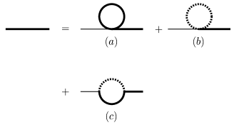
Figure 20: Schematic representation of the selfenergy contribution to pion propagator. Continuous lines correspond to pion propagator, and dashed lines to sigma. The thick line represents the full propagator.

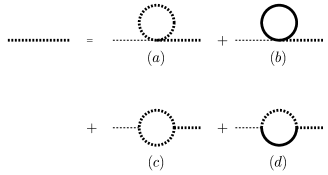
Figure 21: Schematic representation of the self–energy contribution to sigma propagator. Continuous lines correspond to pion propagator, and dashed lines to sigma. Thick line represents the full propagator.

As discussed in the Section I, in the real time formalism, the thermal boson propagator becomes a two by two matrix, but at the level at which we are working we need only the (1,1) component (we ommit the index 11 for simplicity) Leutwyler:1990uq ; Banerjee:1991fu . This is precisely the real time propagator, as given by Dolan and Jackiw Dolan:1974qd . This propagator consists of a sum of two parts: a zero temperature part which corresponds to

$$\mathcal{D}_{0}(k)=\frac{i}{k^{2}-m^{2}+i\epsilon}=i\textbf{P}\frac{1}{k^{2}-m^{2}}+\pi\delta(k^{2}-m^{2})~{},$$ (112)

where P means the principal value, and a thermal part given by

$$\mathcal{D}_{T}(k,T)=2\pi\delta(k^{2}-m^{2})n(k_{0})~{},$$ (113)

where $n(k_{0})$ is the Bose–Einstein distribution function

$$n(k_{0})=\frac{1}{\exp(\beta\;|k_{0}|)-1}~{},$$ (114)

where the factror $\beta=1/T$ defines the inverse temperature while $k_{0}=\sqrt{\textbf{k}^{2}+m^{2}}$ is the energy.

The first part of the propagator is the usual virtual particle exchange, present for all four–momenta $k$. The second term, the thermal part, of the propagator describes real (on shell) particles existing in the hot plasma. These particle particles are present only when $k^{2}=m^{2}$ as the delta fuction constrains Rivers:1994rz . In what follows, we denote the zero temperature part with continuous lines, and the thermal part with lines incorporating a cut “ $|$ ”.

In this part of the work, we cannot follow blindly the same recipe as in the Hartree case using a dressed propagator. The reason is that now the self–energy is momentum dependent as it is obvious from the graph in Fig. 20c, and the ones in Fig. 21c,d . We can avoid this difficulty, if we adopt a “Hartree like” recipe and accept a form of the dressed propagator as

$$G_{\pi/\sigma}(\phi,M)=\frac{1}{K^{2}-M^{2}_{\pi/\sigma}}~{},$$ (115)

where we will consider this effective mass as obtained from the self–energy for zero external momenta.

If we try to distinguish the thermal from the quantum fluctuations, the pion full propagator could be represented by the following set of graphs as is shown in Fig. 22 . On the other hand the full sigma propagator will be represented as is shown in the Fig. 23 .

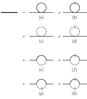
Figure 22: Schematic representation of the self–energy contribution to pion propagator. Continuous lines represent pions, dashed lines are sigmas, and lines with vertical dashes correspond to the thermal propagators.

Figure 23: Schematic representation of the self–energy contribution to sigma propagator. Continuous lines represent pions, dashed lines are sigmas, and lines with vertical dashes correspond to thermal propagators.

IV.3 The pion gap equation

In our attempt to extend the Hartree approximation, our guide is the result of the low–energy theorem which was presented in the first chapter. We have shown that the invariant amplitude of the sum of all four diagrams in Fig. 1 vanishes. This acts as motivation to consider the equivalent in the case where we deal with thermal particles. As a first step, we concetrate at the low–temperature region and mainly on the effects of the sunset diagrams on the effective masses of the pions.

We have shown the sunset diagrams which contribute to the effective potential in Fig. 19. We can redraw these diagrams indicating the thermal propagators with a cut as we did in the graphic representation of the gap equations. These graphs should have the same topology as in Fig. 19, but with one, two or three cut lines representing thermal propagators. There is no graph with 3 thermal sigmas, because of energy conservation at the vertex. We show the complete set of sunset diagrams in Fig. 24 .

Figure 24: Schematic representation of the sunset graphs. Continuous lines represent pions, dashed lines are sigmas, and lines with vertical dashes correspond to thermal propagators.

As a first approximation in the resummation of the subclass of the sunset diagrams, we only consider the sunset diagram with two thermal pions. Our motivation stems from the fact that at zero temperature and in the exact chiral limit, the pions being true Goldstone bosons have vanishing scattering amplitude as was presented in the first chapter. As is shown in Fig. 25, the sunset diagram with two thermal pions corresponds to the case where two real (thermal) pions collide to form a sigma, which afterwards decays into two pions. It also corresponds to pion elastic scattering with sigma exchange.

The sunset diagram with two thermal pions is given in Fig. 25a, and contributes the following term in the effective potential

$$V_{\textrm{s}unset}(\phi,G_{\sigma},G_{\pi})=\frac{\lambda^{2}\phi^{2}}{9}\mathcal{G}_{\pi}^{\theta}(\phi;k)\mathcal{G}_{\pi}^{\theta}(\phi;p)\mathcal{G}_{\sigma}(\phi;k+p)$$ (116)

where $\mathcal{G}$ is an shorthand form of the integral

$$\mathcal{G}_{\pi/\sigma}(\phi;k)=\int_{\beta}G_{\pi/\sigma}(\phi;k)$$ (117)

Propagators indicated as $G^{\theta}$ correspond to the thermal part of the real time propagator given by Eq. (113) .

Figure 25: (a) The sunset diagram with two thermal pions. A line with a dash corresponds to the thermal part of the full propagator. (b)-(d) The equivalent scattering diagrams involving thermal pions.

The full expession corresponding to the diagram in Fig. 25a is

$$I_{\sigma\pi_{\theta}\pi_{\theta}}(M_{\pi},M_{\sigma}) = \int\frac{d^{4}K}{(2\pi)^{4}}\int\frac{d^{4}P}{(2\pi)^{4}}2\pi\,n(k_{0})\;2\pi\,n(p_{0})$$ (118)

$$\times\frac{\delta(K^{2}-M_{\pi}^{2})\,\delta(P^{2}-M_{\pi}^{2})}{(P+K)^{2}-M_{\sigma}^{2}}~{},$$

Following Arnold and Espinosa Arnold:1992rz , we adopt the convenient notation $K^{\mu}=(k_{0},\textbf{k})$, for the four–momenta and, reserve the symbol $k=|\textbf{k}|$, for the magnitude of the three momentum. In this section we have adopted a different formalism than in Sections II and III so the superscripts denote to which particle’s self–energy we are reffered to, while the subscripts denote which particles are running in the loop. A subscript $\theta$ denotes a thermal propagator.

Taking the derivatives of the potential with respect to the full propagator $G_{\pi}$, we get the diagrammatic equation for the pion prapagator given in Fig. 22 . As a first approximation we make a selective summation by including the two graphs as in Hartree (Figs. 22b, d), plus the graph with one thermal pion (Fig. 22f). The topology of this last graph is given in Fig. 26 .

Figure 26: The pion self–energy diagram with one thermal pion.

If we use the real time form of the propagator as in Eqs. (112) and (113), the graph in Fig. 26 contributes with the following expression

$$I^{\pi}_{\sigma\pi_{\theta}}(M_{\pi},M_{\sigma})=\int\frac{d^{4}K}{(2\pi)^{4}}\frac{2\pi n(E_{\pi})\delta(K^{2}-M_{\pi}^{2})}{(P+K)^{2}-M_{\sigma}^{2}+i\epsilon}~{}.$$ (119)

Then using Eq. (112), we can split the above integral into real and imaginary parts. The imaginary part is related to dissipation phenomena that occur as the particles propagate within the thermal plasma. We comment on these matters in Section V where we compare our approach to the chiral phase transition to the work of other investigators.

At the moment, we are interested only in the real part of the above integral, which has the form

$$P(M_{\pi},M_{\sigma})=\int\frac{d^{4}K}{(2\pi)^{4}}\frac{2\pi n(E_{\pi})\delta(K^{2}-M_{\pi}^{2})}{(P+K)^{2}-M_{\sigma}^{2}}~{}.$$ (120)

Evaluation of this integral is given in Appendix D. Then the resulting gap equation for the pions is

$$M_{\pi}^{2} = m^{2}+\frac{1}{6}\lambda\phi^{2}+\frac{\lambda}{6}F(M_{\sigma})+\frac{5\lambda}{6}F(M_{\pi})$$ (121)

$$+\frac{\lambda^{2}\phi^{2}}{9}P(M_{\pi},M_{\sigma})~{}.$$

Taking the derivative of potential with respect to the order parameter results in the following equation

$$0 = m^{2}+\frac{1}{6}\lambda\phi^{2}+\frac{\lambda}{2}F(M_{\sigma})+\frac{\lambda}{2}F(M_{\pi})$$ (122)

$$+\frac{\lambda^{2}}{3}R(M_{\pi},M_{\sigma})~{},$$

where the last term comes from the sunset diagram given in Fig. 25a .

Combining the above equations, we find that the thermal pion mass is given by

$$M_{\pi}^{2} = -\frac{\lambda}{3}F(M_{\sigma})+\frac{\lambda}{3}F(M_{\pi})$$ (123)

$$+\frac{\lambda^{2}\phi^{2}}{9}P(M_{\pi},M_{\sigma})+\frac{\lambda^{2}}{3}R(M_{\pi},M_{\sigma})~{}.$$

As a first step we are interested in the low–temperature phase, and since sigma is very heavy, we do not expect significant changes in the sigma mass, so we can use that $M^{2}_{\sigma}=\frac{1}{3}\lambda\phi^{2}$. Also the contribution from $F(M_{\sigma})$ can be neglected as a first approximation, since it is exponentially supressed. Therefore in order to find out how the pion efective mass evolves with temperature, we need to calculate the terms $R$ and $P$.

Evaluating the integral which corresponds to the pion self–energy graph in Fig. 26, we find

$$P(M_{\pi},M_{\sigma}) = \frac{1}{2\pi^{2}}\int_{0}^{\infty}k^{2}\;dk\frac{n(E_{\pi}^{k})}{E_{\pi}^{k}}$$ (124)

$$\times\frac{2M_{\pi}^{2}-M_{\sigma}^{2}}{(2M_{\pi}^{2}-M_{\sigma}^{2})^{2}-4M_{\pi}^{2}(E_{\sigma}^{k})^{2}}~{}.$$

Details of this calculation can be found in Appendix D. On the other hand, evaluation of the sunset integral in Fig. 25a, results in

$$R(M_{\pi},M_{\sigma}) = -\frac{1}{2(2\pi)^{4}}\int_{0}^{\infty}k\;dk\;g(k,M_{\pi})$$ (125)

$$\times\int_{0}^{\infty}p\;dp\;g(p,M_{\pi})$$

$$\times\ln\frac{X(k,p,M_{\pi},M_{\sigma})}{Y(k,p,M_{\pi},M_{\sigma})}$$

where

$$X(k,p,M_{\pi},M_{\sigma}) = M_{\pi}^{2}(k^{2}+p^{2})+M^{2}_{\sigma}(M_{\pi}^{2}-M^{2}_{\sigma}/4)$$

$$+(2M^{2}_{\pi}-M^{2}_{\sigma})kp~{},$$

$$Y(k,p,M_{\pi},M_{\sigma}) = M_{\pi}^{2}(k^{2}+p^{2})+M^{2}_{\sigma}(M_{\pi}^{2}-M^{2}_{\sigma}/4)$$

$$-(2M^{2}_{\pi}-M^{2}_{\sigma})kp$$

and we have used the abbreviatiated form for $g(p,M)$ introduced by Eq. (68). The exact calculation is given in Appendix F.1 .

It is interesting to see how these integrals behave in the limit of vanishing pion mass. Using a compact notation (introduced in Section I), $F(M)$ can be written as

$$F(M_{\pi/\sigma})=\frac{T^{2}}{2\pi^{2}}f(M_{\pi/\sigma}/T)~{}.$$ (126)

Rescaling the integral as $x=\beta k$, and in the limit of vanishing pion masses, we obtain the following expressions for the real part of the above integral, corresponding to self–energy graph

$$P(M_{\pi},M_{\sigma}) = -\frac{1}{M_{\sigma}^{2}}\frac{T^{2}}{2\pi^{2}}\int_{0}^{\infty}g(x,M_{\pi}/T)$$ (127)

$$= -\frac{1}{M_{\sigma}^{2}}\frac{T^{2}}{2\pi^{2}}f(M_{\pi}/T)~{}.$$

On the other hand, the integral corresponding to sunset graph is given by

$$R(M_{\pi},M_{\sigma}) = -\frac{1}{2(2\pi)^{2}}\frac{8T^{4}}{M_{\sigma}^{2}}\int_{0}^{\infty}x^{2}dx\;g(x,M_{\pi}/T)$$ (128)

$$\times\int_{0}^{\infty}y^{2}dy\;g(y,M_{\pi}/T)~{}.$$

Recall now that the sigma mass is given by

$$M^{2}_{\sigma}=\frac{1}{3}\lambda\phi^{2}~{}.$$ (129)

Inserting these into the pion gap equation, we can observe that $F(M_{\pi})$ and $P(M_{\pi},M_{\sigma})$ cancel exactly, so we end up with an expession where the thermal contribution to the pion mass squared is $\mathcal{O}(T^{4})$. The same result under a different approach has already been reported by Itoyama and Mueller Itoyama:1983up  .

We illustrate the situation with in Fig. 27, where we plot the pion mass as we have calculated above, with the effective pion mass as was calculated in Hartree approximation. As we can observe in Fig. 27, in the Hartree calculation the pion mass is proportional to temperature. In contrast, inclusion of the self–energy graph results in the mass being $\sim T^{2}$ and obviously is small at low temperatures.

Figure 27: The low–temperature pion mass $M_{\pi}$, as a function of temperature. The continuous line corresponds to the Hartree approximation.

IV.4 The sigma gap equation

In our attempts to consider all the self–energy graphs with one thermal particle in the loop, we faced serious numerical difficulties mainly from the pion self–energy graph. Being unable to solve the complete system of equations, we have tried to understand the effects of each one graph individually.

If we add to the potential the sunset with two thermal sigmas, which is given in the Fig. 28, differentiating, we find a gap equation for sigma which contains the contribution of the sigma self–energy graph given in Fig. 29.

Figure 28: The sunset diagram with two thermal sigmas. A line with a dash corresponds to the thermal part of the full propagator.

Figure 29: The sigma self–energy diagram, with one thermal sigma.

We proceed, using the same system of equations as in Hartree, with the only difference being that the sigma gap equation will contain the contribution of this graph. We have also introduced the symmetry breaking term, so the pions are massive. The result, given in Fig. 30, is somehow the one expected. We know that the sigma is heavy so, at low temperatures, there is no significant difference with the Hartree calculation. On the other hand, at high temperatures the masses will approach ideal gas behaviour. Only in the intermediate region of temperatures we can observe a small deviation of the Hartree result.

Figure 30: Solution of the system of gap equations for the sigma and pion effective masses. Dashed lines correspond to the Hartree solution as in Section II. The pion gap equation is as in the Hartree case, while in the equation for the sigma we have included the sigma self–energy graph with one thermal sigma.

There is also no problem in calculating the sigma self–energy graph with one thermal pion given in Fig. 31. However, the addition of the relevant term into the sigma gap equation deviates the sigma mass from $m_{\sigma}=600\;\textrm{MeV}$ as it is clear in Fig. 32 . We suspect that this is due to the fact that we do not include the vacuum graphs.

Figure 31: The sigma self–energy diagram with one thermal pion.

Figure 32: Solution of the system of gap equations for the sigma and pion effective masses. Dashed lines correspond to Hartree solution as in Section II. The pion gap equation is as in the Hartree case, while in the equation for the sigma we have included the sigma self–energy graph with one thermal pion.

V Other approaches

V.1 Propagation of pions in hot plasmas

Self–consistent approximations in many body systems have been tried a long time ago. To our knowledge, these attempts date back to the 1960’s, with early papers such as the ones by Luttinger and Ward Luttinger:1960 , or the ones by Baym Baym:1962 . Recently these ideas have been employed by many people in various contexts as in the recent works by Knoll, Van Hees and others vanHees:2000bp ; Ivanov:2000ma .

Our approach to the chiral phase transition is not, of course, the only one. There have been a lot of studies on the subject since it is related to important phenomena as the formation of quark–gluon plasma, the dilepton emmision etc. People have used various ways to approach these problems, and we are going to outline their success here.

A basic ingredient for the understanding of several physical processes that take place in hadronic plasmas, is the propagation properties of pions. The properties of pions in hot hadronic matter are encoded in the pion propagator. The real part of the pion self energy is related to dispersion and group velocity, while the imaginary part encodes the information about the pion absorption Goity:1989gs ; Schenk:1993ru ; Pisarski:1996mt . In general, the expression which gives the pion mass shift is of the form

$$(p^{0})^{2}=\bm{p}^{2}+M_{\pi}^{2}+\Sigma(p^{0},\bm{p})~{},$$ (130)

where $\Sigma$ is the pion self energy, and it depends on the physical conditions of the medium, in which the pion propagates.

At the one loop level as it is the Hartree approximation there is no imaginary part in the self energy. The effective mass of the particles acquires just thermal contribution. However, when we include the sunset diagrams into the potential the mass gap equations contain terms which are momentum dependent.

A recent work, which uses the linear sigma model in order to study dissipation phenomena in hot matter, is the one by Ayala, Sahu and Napsuciale Ayala:2000ry ; Ayala:2000px ; Ayala:2000bx  . Another work about dissipation properies of the pions, is the one by Rischke Rischke:1998qy . The pion self–energy is calculated at the one–loop level. In order to perform the study, the momentum running in the loop is divided into soft and hard. The model is used to study disoriented chiral condensates.

V.2 Other approaches using the sigma model

The linear sigma model is a rich theory in its own right, however it has been used as an effective theory to QCD transition since direct QCD calculations are very complicated. The model has been used in various approaches of the QCD phase transition, both in and out of equilibrium. It has been especially popular in studies involving the formation of disoriented chiral condensates. The formation of DCC was proposed long ago, as a signal of the chiral phase transition Bjorken:1992xr .

The CJT method and the linear sigma model have been used in other recent investigations, too. Our approach to the chiral phase transition appears to be complementary in most of these approaches. Throughout this report, we have not discussed the issue of renormalization. It is well known that the linear sigma model is renormalizable at zero temperature. However, recent attempts to incorporate renormalization at finite temperature, have not always been successful. An attempt by Amelino–Camelia Amelino-Camelia:1997dd , to examine renormalization of the linear sigma model at finite temperature results in violation of the Goldstone theorem. We have mentioned this already in the third section. A recent successful treatment of the renormalization matters, is the one by Rischke and Lenaghan Lenaghan:2000si .

In the Hartree approximation, we have calculated the effective masses of sigma and the pions. We call them effective masses, since they correspond to the modification of the bare particle masses, which result after their “in medium ” interactions. Of course, they do not correspond to the real observed masses, since in our approach, we have ignored quantum fluctuations throughout this work.

In the work of Chiku and Hatsuda Chiku:1998va ; Chiku:1998kd , the optimal perturbation theory is employed in order to perform the calculations. They obtained gap equations for the effective masses, which go further than our Hartree approximation. They include quantum fluctuations as well. So we cannot really compare our results in full. However, they do not calculate the effective potential.

In the work of Nemoto, Naito and Oka Nemoto:1999qf , there are many similarities to our approach. First of all, the CJT method is used for the calculations, however they renormalize the model, and use a definition for the particle masses as the minimum of the potential.

In the work of Caldas, Mota and Nemes Caldas:2000ic , the main difference is that they do include fermions as well. Their calculation of evolution of the condensate look very similar to our result. The show a first–order phase transition in the chiral limit, and a crossover when there is an explicit breaking of chiral symmetry. In the work of Bilic and Nicolic Bilic:1995ic , they also include fermions, and find a first–order phase transition.

Bochkarev and Kapusta Bochkarev:1996gi , have focused in the differences between the linear and non–linear sigma model. They use the $O(N)$ version, and their result is similar to our large–$N$ approximation, since they found a second–order phase transition as well. They also find that the non–linear sigma model has a second–order phase transition as well.

VI Summary of the results

VI.1 Conclusions

We have studied the chiral phase transition using the linear sigma model. In order to understand the nature of the phase transition and how it could proceed, in the first two sections of this work, we have calculated the finite temperature effective potential of this model in the Hartree and large–$N$ approximations using the CJT formalism of composite operators. This method has the advantage that we actually only need to calculate one type of diagram.

In both cases, we solved the system of gap equations numerically, and found the evolution with temperature of the thermal effective masses. In the Hartree approximation, we find a first–order phase transition but, in contrast, the large $N$ approximation predicts a second–order phase transition. This last observation seems to be in agreement with different approaches to the chiral phase transition based on the argument that the linear sigma model belongs in the same universality class as other models, which are known to exhibit second order phase transitions Rajagopal:1993ah .

However, in the large–$N$ approximation, the sigma contribution is ignored and this, of course, introduces errors when we calculate the critical temperature. We found that the large–$N$ approximation predicts a higher transition temperature than the Hartree one. However, we have concluded that this is an artefact of the calculation, since both Hartree and large–$N$ approximations should have the same high temperature limit. We should recall that, we can calculate the transition temperature by considering the high temperature limit from the mass gap equation, since it is defined as the temperature where the particles become massless. As we have pointed out in Section II, in both cases and at high temperatures the behaviour of the pion–sigma system approches that of the ideal gas.

When we include the symmetry breaking term $\varepsilon\sigma$ which generates the observed pion masses, we found that there is no longer any phase transition, both in Hartree and large–$N$ approximations. Instead, we observe a crossover phenomenon, where the change of the order parameter in the Hartree case occurs more rapidly in contrast to the smoother behaviour exhibited in the large–$N$ approximation. Our observation confirms results reported recently by Chiku and Hatsuda Chiku:1998va ; Chiku:1998kd using the ideas of optimal perturbation theory. In their analysis they also report indication of a first order phase transition in the chiral limit. This observation is closer to the real world, since the pions are only approximately Goldstone bosons.

Of course, as we have already pointed out, the linear sigma model is only an approximation to the real problem which is QCD, but the study of the chiral phase transition in the framework of this model could be a helpful guide to how one could tackle the original problem, and get some insight in the physics involved. For the calculations both in Hartree and large–$N$ approximations, we have used the imaginary time formalism which is adequate for studies at thermal equilibrium but if one is interested in studies of the dynamics of the phase transition, the real time formalism seems to be more convenient Smilga:1997cm . We did not study the system far from equilibrium, however the real time formalism would allow us to extend the investigation, and consider the dynamics of the system. In real time formalism, we have the advantage that the propagator splits into two parts from the beginning, so making it easier to calculate thermal corrections to the effective masses.

However, our attempt to go futher than the Hartree approximation has run into serious difficulties. It is not absolutely clear which class of diagrams we should consider. Our motivation to include only the sunset–type diagrams with two thermal particle only, comes out from conciderations of the low–energy theorem, and our percistence into symmetry principles. This is why we have not tried to renormalise the model as well. It is well known that the linear sigma model is a renormalizable theory at zero temperature, and that finite temperature effects do not indroduce new divergencies – at least at the ultraviolet –, since the temperature acts as a natural cut–off. However, renormalization of the model is investigated in other recent investigations as it was mentioned already.

The fact that near the transition temperature, the effect of higher loops may become important, it is well known for a long time, and suggests that further investigation is needed. We would suggest that an extension of our two loop calculation is tractable, provided one takes into account the efffects of all the loops contributing at the two–loop level, as a first step. However, it is not clear how the CJT method could be used to include the effects of higher loops. Selfconsistent approximations have been used for a long time, but it is not clear how they work beyond the one loop level.

VI.2 Some recent results

We conclude this work reviewing some recent progress on the subject. Since the work which presented in the previous sections was initially written, there has has been quite some progress on similar studies. The linear sigma model has always been a very popular model in studies attempting to mimic the most of the low energy region of QCD.

Perhaps the most interesting result, which is related to this work and has been published recently, is the work of Baacke and Michalski Baacke:2002pi , where the authors examine the $O(N)$ linear sigma model beyond the Hartree approximation. The same authors have also studied the sigma model at non–equilibrium in Baacke:2001zt (see also Michalski:2003fp ). However, it seems that their approach does not suffer from the difficulties that we have faced trying to solve the full system of gap equations at the two loop level of the effective potential. An essential difference between our approach and the one by Baacke and Michalski is the renormalisation of the model. As we have seen already in Section I the CJT method is based on a resummation of the 2PI graphs. The analysis of Baacke:2002pi is based on the a variation of the CJT method, which is called 2PPI resummation. This method has been initiated by Verschelde and Coppens Verschelde:bs and it is presented in a number of papers Verschelde:2000dz ; Verschelde:2000ta ; Smet:2001un .

In order to study the effective potential Baacke and Michalski have calculated the full subset of sunset diagrams. This of course makes their approach more complete. However, our attempt was focused mainly on the sunset with two thermal pions trying to test if the low energy theorem has an analogy at finite temperature, rather than tackling issues like for example renormalization of the model at the full two loop calculation, or attempts to consider the full two loop case.

An alternative approach to the problem of the selfconsistent approximations, is the work of Knoll and van Hees vanHees:2001ik ; VanHees:2001pf ; vanHees:2002bv where they use the $\Phi$ derivable approximation. This method orinates from the work of Baym Baym:1962 and it has essentially many similarities with CJT. However, it seems that renormalisation is controlled better under this calculational scheme.

The CJT method is an attractive framework in order one to perform selfconsistent approximations and has attracted quite some attention. The method is used in a recent paper by Roder et al Roder:2003uz where the authors study restoration of chiral symmetry and the low lying meson spectrum at finite temperature. Also in another recent study of the $O(4)$ linear sigma model Phat et al Phat:2003eh have used the CJT method as well. In their analysis, in contrast to our approach, they have studied the issue of renormalisation while they have incorporated the effects od higher loops. Other recent work on the $O(N)$ linear sigma model, but without using CJT, is the work of Patkos et al Patkos:2002ec ; Patkos:2002vr ; Patkos:2002vq ; Patkos:2002xb where they study the behaviour of the spectal functions, as well as, the position of the sigma pole on the complex energy plane.

Appendix A The potential at one–loop

In this appendix, we review the calculation of the one–loop contribution to the effective potential for a $\lambda\phi^{4}$ theory, using the imaginary time formalism. This is a well presented calculation, and appears in many research papers and textbooks, as for example references Dolan:1974qd ; Kapusta:1989 ; Das:1997gg . However, in order to make this presentation more self–contained, and also compare it with the real time calculation, we will reproduce the basic steps here. The propagator is given by

$$\mathcal{D}^{-1}(\phi;k)=k^{2}+m^{2}~{}.$$ (131)

The one loop contribution to the effective potential is of the form

$$V(\phi,T) = \int_{\beta}d^{4}k\,\ln\mathcal{D}^{-1}(k;\phi)$$ (132)

$$= -\frac{1}{2\beta}\sum_{n}\int\frac{d^{3}\textbf{k}}{(2\pi)^{3}}\ln(k^{2}+m^{2})$$

$$= -\frac{1}{2\beta}\sum_{n}\int\frac{d^{3}\textbf{k}}{(2\pi)^{3}}\ln\left(\frac{4n^{2}\pi^{2}}{\beta^{2}}-E^{2}\right)~{},$$

where $E^{2}=\textbf{k}^{2}+m^{2}$, and we have indicated the sum over the Matsubara frequency $k_{0}=\omega_{n}=2\pi n\beta^{-1}$ explicitly. We should recall that $\beta=1/T$, where $T$ is the temperature.

In order to evaluate this sum we can define

$$u(E)=\sum_{n}\ln\left(\frac{4n^{2}\pi^{2}}{\beta^{2}}+E^{2}\right)$$ (133)

so the derivative is

$$\frac{\partial u(E)}{\partial E}=\sum_{n}\frac{2E}{4n^{2}\pi^{2}/\beta^{2}+E^{2}}~{}.$$ (134)

We can now use the formula Gradshteyn:1980

$$\sum_{n}\frac{x}{x^{2}+n^{2}}=-\frac{1}{2x}+\frac{1}{2}\pi\coth\pi x~{},$$ (135)

to find that

$$\frac{\partial u(E)}{\partial E}=2\beta\left(\frac{1}{2}+\frac{1}{e^{\beta E}-1}\right)~{},$$ (136)

and

$$u(E)=2\beta\left(\frac{E}{2}+\frac{1}{\beta}\ln(1-e^{\beta E})\right)~{}.$$ (137)

The result is summarised as

$$V(\phi,T) = V^{0}(\phi)+V^{\beta}(\phi)$$

$$= \int\frac{d^{3}\textbf{k}}{(2\pi)^{3}}\frac{E}{2}+\frac{1}{\beta}\int\frac{d^{3}\textbf{k}}{(2\pi)^{3}}\ln(1-e^{-\beta E})~{}.$$

Appendix B One loop mass correction

We have seen in n Section I, that the one–loop correction to scalar propagator only causes a mass shift. The relevant graph is shown in Fig. 33 .

Figure 33: The self–energy contribution to scalar propagator.

This graph involves evaluation of the following integral

$$F(m) = -\frac{1}{2\beta}\sum_{n}\int\frac{d^{3}\textbf{k}}{(2\pi)^{3}}\frac{1}{(2n\pi/\beta)^{2}+E^{2}}$$

$$= -\frac{1}{2\beta}\left(\frac{\beta}{2\pi}\right)^{2}\sum_{n}\int\frac{d^{3}\textbf{k}}{(2\pi)^{3}}\frac{1}{n^{2}+(\beta E/2\pi)^{2}}~{}.$$

If we use the formula

$$\sum_{n}\frac{1}{x^{2}+n^{2}}=\frac{\pi}{x}+\coth\pi x~{},$$ (140)

we find that

$$F(m)=-\frac{1}{2}\int\frac{d^{3}\textbf{k}}{(2\pi)^{3}}\frac{1}{2E}\coth\left(\frac{\beta E}{2}\right)~{}.$$ (141)

From the fact that

$$\coth\beta x=1+2n(2x)~{},$$ (142)

where $n(E)$ is the Bose–Einstein distribution function

$$n(E)=\frac{1}{e^{\beta E}-1}~{},$$ (143)

we find that he above integral is written as a sum of two parts

$$F(m) = F_{0}(m)+F_{\beta}(m)$$

$$= \frac{1}{2}\int\frac{d^{3}\textbf{k}}{(2\pi)^{3}}\frac{1}{2E}+\frac{1}{2}\int\frac{d^{3}\textbf{k}}{(2\pi)^{3}}\frac{1}{E}\frac{1}{e^{\beta E}-1}~{}.$$

Appendix C The Keldysh contour

The imaginary time or Matsubara formalism has the disadvantage that if one wants to calculate non equilibrium quantities, an analytic continuation to real time must be performed. In this formalism, we are integrating in the complex plane of the Minkowski time, from $t=0$ to $t-i\beta$. The periodicity of the fields enables us to generalise this interval to, $t_{0}$ to $t_{0}-i\beta$, for any real $t_{0}$.

Alternatively, one can work directly in real time. In this case, we need a different choice of contour with the same endpoints which will contain the real time axis. A choice of contour for time integration, which is called the Keldysh contour, is shown in Fig. 34.

Figure 34: Keldysh contour

As we can see in Fig. 34, the Keldysh contour consists of four pieces. However, there is an alternative choice of contour Evans:1995gb . For analyticity reasons, it can be shown that the contributions from $C_{3}$ and $C_{4}$ can be neglected. Therefore, we are left with two possibilities for both the initial and final points of integration to lie either on $C_{1}$ or $C_{2}$. This gives four different propagators, which are usually written in matrix form. We have given these propagators in Section I.4.

Appendix D The pion self–energy graphs

D.1 The pion self–energy graph with one thermal pion

Although the calculation of the self–energy graphs for $\lambda\phi^{4}$ is a well known subject, and appears in many research papers, we repeat the derivation here, hoping to make the presentation of the calculations more complete. Evaluation of the self–energy can be done using any of the formalisms: imaginary time, real time or thermo–field dynamics LeBellac:1996 ; Contreras:1990gi ; Arnold:1993qy ; Weldon:1983jn ; Fujimoto:1986me . We find the real time convenient at this stage. The pion self–energy graph with one thermal pion in the loop, is given in Fig. 35.

As mentioned already in Section IV, in our case, we need only the (1,1) component of the matrix propagator. This has a zero temperature part

$$\mathcal{D}_{0}(k)=\frac{i}{k^{2}-m^{2}+i\epsilon}=i\textbf{P}\frac{1}{k^{2}-m^{2}}+\pi\delta(k^{2}-m^{2})~{},$$ (145)

where P means the principal value, and a thermal part given by

$$\mathcal{D}_{T}(k,T)=2\pi\delta(k^{2}-m^{2})n(k_{0})$$ (146)

where $n(k_{0})$ is the Bose–Einstein distribution function

$$n(k_{0})=\frac{1}{\exp(\beta\;|k_{0}|)-1}~{},$$ (147)

with $\beta=1/T$ the inverse temperature and $k_{0}=\sqrt{\textbf{k}^{2}+m^{2}}$.

Figure 35: The pion self–energy diagram with one thermal pion.

We use the following convention for 4–momenta $K^{\mu}=(k_{0},\textbf{k})$, and reserve $k$ for the magnitude of the 3-momentum, so $k=|\textbf{k}|$. Since we are interested in the real part of the self–energy graph, we ignore the second part of the vacuum propagator (the one with the delta function). Then the exact expression corresponding to the graph in Fig. 35 is written as

$$I^{\pi}_{\sigma\pi_{\theta}}(M_{\pi},M_{\sigma})=\int\frac{d^{4}K}{(2\pi)^{4}}\frac{2\pi n(k_{0})\delta(K^{2}-M_{\pi}^{2})}{(P+K)^{2}-M_{\sigma}^{2}}~{}.$$ (148)

As we have mentioned earlier, the superscripts denote to which particle’s self–energy we are reffered to, while the subscripts denote which particles are running in the loop. A subscript $\theta$ denotes a thermal propagator.

By using partial fractioning, we can write the above integrand as

$$\frac{1}{(P+K)^{2}-M_{\sigma}^{2}} = \frac{1}{2E_{\sigma}^{k+p}}\bigg{[}\frac{1}{p_{0}+k_{0}-E_{\sigma}^{k+p}}$$

$$-\frac{1}{p_{0}+k_{0}+E_{\sigma}^{k+p}}\bigg{]}~{}.$$

Where the superscript in the expression for the energy has the obvious meaning, $E^{q}_{a}=\sqrt{q^{2}+m^{2}_{a}}$. In order to perform the integration, we use the following property of the Dirac delta function

$$\delta(x^{2}-a^{2})=\frac{1}{2|a|}\bigg{[}\delta(x+a)+\delta(x-a)\bigg{]}~{}.$$ (149)

Inserting everything in the integral, and integrating over the delta function, results in

$$I^{\pi}_{\sigma\pi_{\theta}}(M_{\pi},M_{\sigma}) = \frac{1}{2\pi^{2}}\int_{0}^{\infty}k^{2}dk\frac{n(E_{\pi}^{k})}{2E_{\pi}^{k}E_{\sigma}^{k+p}}$$

$$\;\;\;\;\times\bigg{[}\frac{1}{p_{0}+E_{\pi}^{k}-E_{\sigma}^{k+p}}$$

$$\;\;\;\;\;-\frac{1}{p_{0}+E_{\pi}^{k}+E_{\sigma}^{k+p}}$$

$$\;\;\;\;\;+\frac{1}{p_{0}-E_{\pi}^{p}-E_{\sigma}^{k+p}}$$

$$\,\;\;\;\;-\frac{1}{p_{0}-E_{\pi}^{k}+E_{\sigma}^{k+p}}\bigg{]}~{},$$

or, in a more compact form, as

$$I^{\pi}_{\sigma\pi_{\theta}}(M_{\pi},M_{\sigma}) = \frac{1}{2\pi^{2}}\int_{0}^{\infty}k^{2}dk\frac{n(E_{\pi}^{k})}{E_{\pi}^{k}}$$

$$\times\bigg{[}\frac{1}{(p_{0}+E_{\pi}^{k})^{2}-(E_{\sigma}^{k+p})^{2}}$$

$$\;\;\;\;+\frac{1}{(p_{0}-E_{\pi}^{k})^{2}-(E_{\sigma}^{k+p})^{2}}\bigg{]}~{}.$$

In the case when we consider pions as static, then ${\textbf{p}=0}$ and so $p_{0}=M_{\pi}$, therefore we can write the above as

$$I^{\pi}_{\sigma\pi_{\theta}}(M_{\pi},M_{\sigma}) = \frac{1}{4\pi^{2}}\int_{0}^{\infty}k^{2}\;dk\frac{n(E_{\pi}^{k})}{E_{\pi}^{k}}$$ (150)

$$\times\bigg{[}\frac{1}{(M_{\pi}+E_{\pi}^{k})^{2}-(E_{\sigma}^{k})^{2}}$$

$$\;\;\;\;+\frac{1}{(M_{\pi}-E_{\pi}^{k})^{2}-(E_{\sigma}^{k})^{2}}\bigg{]}~{},$$

or even as

$$I^{\pi}_{\sigma\pi_{\theta}}(M_{\pi},M_{\sigma}) = \frac{1}{2\pi^{2}}\int_{0}^{\infty}k^{2}\;dk\frac{n(E_{\pi}^{k})}{E_{\pi}^{k}}$$ (151)

$$\times\frac{2M_{\pi}^{2}-M_{\sigma}^{2}}{(2M_{\pi}^{2}-M_{\sigma}^{2})^{2}-4M_{\pi}^{2}(E_{\sigma}^{k})^{2}}~{}.$$

D.2 The pion self–energy graph with one thermal sigma

Another graph which contributes to the pion self–energy, is the one given in Fig. 36. As we can easily observe, apart from that the thermal particle is a sigma now, this graph is absolutely analogous to the one presented above. Therefore, following the same procedure as before, we end up with the following expression

Figure 36: The pion self-energy diagram with one thermal sigma.

$$I^{\pi}_{\pi\sigma_{\theta}}(M_{\pi},M_{\sigma}) = \frac{1}{2\pi^{2}}\int_{0}^{\infty}k^{2}\;dk\frac{n(E_{\sigma}^{k})}{E_{\sigma}^{k}}$$ (152)

$$\times\bigg{[}\frac{1}{(M_{\pi}+E_{\sigma}^{k})^{2}-(E_{\pi}^{k})^{2}}$$

$$~{}~{}+\frac{1}{(M_{\pi}-E_{\sigma}^{k})^{2}-(E_{\pi}^{k})^{2}}\bigg{]}$$

Appendix E The sigma self–energy graphs

E.1 The sigma self–energy graph with one thermal sigma

Evaluation of the sigma self–energy graphs can be done in a completely analogous way as to one of the pions. However, since it involves identical particles it is even easier. Therefore,

Figure 37: The sigma self–energy diagram with one thermal sigma.

$$I^{\sigma}_{\sigma\sigma_{\theta}}(M_{\sigma})=\frac{1}{2\pi^{2}}\int_{0}^{\infty}k^{2}\;dk\frac{n(E_{\sigma}^{k})}{E_{\sigma}}\frac{1}{M_{\sigma}^{2}-4E_{\sigma}^{2}}~{}.$$ (153)

E.2 The sigma self–energy graph with one thermal pion

In this case we have the topology as in Fig. 38

Figure 38: The sigma self–energy diagram with one thermal pion.

Evaluating the relevant integral as above, we find

$$I^{\sigma}_{\sigma\pi_{\theta}}(M_{\pi})=\frac{1}{2\pi^{2}}\int_{0}^{\infty}k^{2}\;dk\frac{n(E_{\pi}^{k})}{E_{\pi}}\frac{1}{M_{\pi}^{2}-4E_{\pi}^{2}}~{}.$$ (154)

Appendix F Calculation of sunset graphs

F.1 The sunset with two thermal pions

The sunset diagrams consist of a set of diagrams with the topology given in Fig. 24 . However, in the approximation adopted for this work, we ignore quantum fluctuations, so we do not take into account the graphs with one thermal propagator or none. The graphs with three thermal propagators do not contribute (because of conservation of energy), so we are left only with the graphs containing two thermal propagators.

Figure 39: The sunset diagram, with two thermal pions. A line with a dash corresponds to the thermal part of the full propagator.

In the case of two thermal pions in the sunset as shown in Fig. 39, we deal with the expession

$$I_{\sigma\pi_{\theta}\pi_{\theta}}(M_{\pi},M_{\sigma}) = \int\frac{d^{4}K}{(2\pi)^{4}}\int\frac{d^{4}P}{(2\pi)^{4}}2\pi\,n(k_{0})\;2\pi\,n(p_{0})$$ (155)

$$\times\frac{\delta(K^{2}-M_{\pi}^{2})\,\delta(P^{2}-M_{\pi}^{2})}{(P+K)^{2}-M_{\sigma}^{2}}~{},$$

and in order to evaluate this integral, we use the property of the delta function given by Eq. (149). Then our expression will consist of four terms containing products of delta functions of the form

$$\delta(k_{0}\pm E_{\pi})\delta(p_{0}\pm E_{\pi})~{}.$$ (156)

In order to perform this integration, it is convenient to choose k as defining the polar axis, so then $\theta$ is the angle between the three vectors k and p. Then, the first term of the integral given in Eq. (155) will appear as

$$R_{a}(M_{\pi},M_{\sigma}) = \frac{1}{2(2\pi)^{4}}\int\frac{dk_{0}}{k_{0}}\frac{kdk}{e^{\beta k_{0}}-1}$$

$$\times\int\frac{dp_{0}}{p_{0}}\frac{pdp}{e^{\beta p_{0}}-1}\;\mathcal{A}(k,p,\theta)$$

where we have defined $\mathcal{A}=\mathcal{A}(k,p,\theta)$ as a shorthand of the lengthy expression

$$\mathcal{A}=\frac{kp\sin\theta\;d\theta\;\delta(k_{0}-E_{\pi}^{k})\;\delta(p_{0}-E_{\pi}^{p})}{k_{0}^{2}-k^{2}+p_{0}^{2}-p^{2}+2k_{0}p_{0}-2kp\sin\theta-M_{\sigma}^{2}}~{}.$$

After performing the delta function integration, we end up with the result

$$R_{a}(M_{\pi},M_{\sigma}) = \frac{1}{2(2\pi)^{4}}\int\frac{kdk}{E_{\pi}^{k}}\frac{1}{e^{\beta E_{\pi}^{k}}-1}$$

$$\int\frac{pdp}{E_{\pi}^{p}}\frac{1}{e^{\beta E_{\pi}^{p}}-1}kp\;\mathcal{B}(k,p,\theta)$$

and we have defined again a shorthand expression $\mathcal{B}=\mathcal{B}(k,p,\theta)$ as

$$\mathcal{B}=\frac{kp\sin\theta\;d\theta}{(E_{\pi}^{k}+E_{\pi}^{p})^{2}-k^{2}-p^{2}-2kp\sin\theta-M_{\sigma}^{2}}~{}.$$

Finally, performing the angular intergration, we find

$$R_{a}(M_{\pi},M_{\sigma}) = \frac{1}{2(2\pi)^{4}}\int\frac{kdk}{E_{\pi}^{k}}n(E_{\pi}^{k})\int\frac{pdp}{E_{\pi}^{p}}n(E_{\pi}^{p})$$

$$\times\ln\frac{2\;M_{\pi}^{2}-M^{2}_{\sigma}+2k_{0}\;p_{0}+2kp}{2\;M_{\pi}^{2}-M^{2}_{\sigma}+2k_{0}\;p_{0}-2kp}~{}.$$

In repeating this procedure, there will be four other similar terms, one for each of the combinations of delta functions given by Eq. (156). Then the final result can be written as

$$I_{\sigma\pi_{\theta}\pi_{\theta}}(M_{\pi},M_{\sigma}) = -\frac{1}{2(2\pi)^{4}}\int\frac{kdk}{E_{\pi}^{k}}n(E_{\pi}^{k})\int\frac{pdp}{E_{\pi}^{p}}n(E_{\pi}^{p})$$ (157)

$$\times\ln\frac{A(k,p,M_{\pi},M_{\sigma})}{B(k,p,M_{\pi},M_{\sigma})}$$

where

$$A(k,p,M_{\pi},M_{\sigma}) = M_{\pi}^{2}(k^{2}+p^{2})+M^{2}_{\sigma}(M_{\pi}^{2}-M^{2}_{\sigma}/4)$$

$$+(2M^{2}_{\pi}-M^{2}_{\sigma})kp~{},$$

$$B(k,p,M_{\pi},M_{\sigma}) = M_{\pi}^{2}(k^{2}+p^{2})+M^{2}_{\sigma}(M_{\pi}^{2}-M^{2}_{\sigma}/4)$$

$$-(2M^{2}_{\pi}-M^{2}_{\sigma})kp~{}.$$

F.2 The sunset with two thermal sigmas

In the case when we need to calculate the sunset with two thermal sigmas, the situation will be absolutely analogous to the one presented above for the two pions. The diagram has the topology given in Fig. 40 .

Figure 40: The sunset diagram, with two thermal sigmas. A line with a dash corresponds to the thermal part of the full propagator.

Then the exact expression corresponding to this graph is given by

$$I_{\sigma\sigma_{\theta}\sigma_{\theta}}(M_{\pi},M_{\sigma}) = \int\frac{d^{4}K}{(2\pi)^{4}}\int\frac{d^{4}P}{(2\pi)^{4}}\,2\pi n(k_{0})\;2\pi n(p_{0})$$ (158)

$$\times\frac{\delta(K^{2}-M_{\sigma}^{2})\,\delta(P^{2}-M_{\sigma}^{2})}{(P+K)^{2}-M_{\sigma}^{2}}~{}.$$

In order to evaluate this, we repeat the steps as in case with the two thermal pions. The final result will be of the form

$$I_{\sigma\sigma_{\theta}\sigma_{\theta}}(M_{\pi},M_{\sigma}) = \frac{1}{2(2\pi)^{4}}\int\frac{kdk}{E_{\sigma}^{k}}n(E_{\sigma}^{k})\int\frac{pdp}{E_{\sigma}^{p}}n(E_{\sigma}^{p})$$ (159)

$$\times\ln\frac{4(k+p)^{2}+3M^{2}_{\sigma}+4kp}{4(k+p)^{2}+3M^{2}_{\sigma}-4kp}~{}.$$

References

- (1) L. Mclerran, The Physics Of The Quark Gluon Plasma, Rev. Mod. Phys. 58, 1021 (1986).
- (2) D. J. Gross, R. D. Pisarski and L. G. Yaffe, QCD And Instantons At Finite Temperature, Rev. Mod. Phys. 53, 43 (1981).
- (3) A. V. Smilga, Physics of thermal QCD, Phys. Rept. 291, 1 (1997). [hep-ph/9612347].
- (4) A. D. Linde, Phase Transitions In Gauge Theories And Cosmology, Rept. Prog. Phys. 42, 389 (1979).
- (5) A. D. Linde, Particle Physics and Inflationary Cosmology, Harwood Academic Publishers, (1990).
- (6) K. Rajagopal, The Chiral phase transition in QCD: Critical phenomena and long wavelength pion oscillations, [hep-ph/9504310].
- (7) U. W. Heinz, The little bang: Searching for quark-gluon matter in relativistic heavy-ion collisions, Nucl. Phys. A 685 (2001) 414 [hep-ph/0009170].
- (8) D. H. Rischke, The Quark Gluon Plasma in Equilibrium, [nucl-th/0305030].
- (9) S. B. Ruster and D. H. Rischke, Effect of color superconductivity on the mass and radius of a quark star, [nucl-th/0309022].
- (10) M. C. Birse, Chiral symmetry in nuclei: Partial restoration and its consequences, J. Phys. G G20, 1537 (1994) [nucl-th/9406029].
- (11) L. F. Li, Spontaneous symmetry breaking and chiral symmetry, AIP Conf. Proc. 531 (2000) 16 [hep-ph/0001116].
- (12) T. Hatsuda and T. Kunihiro, Chiral symmetry restoration and the sigma-meson, [hep-ph/0010039].
- (13) T. Kunihiro, Roles of chiral symmetry and the sigma meson in hadron and nuclear physics, [hep-ph/0009116].
- (14) M. Gell-Mann and M. Levy, The Axial Vector Current In Beta Decay, Nuovo Cim. 16, 705 (1960).
- (15) D. A. Kirzhnits, Weinberg Model In The Hot Universe, JETP Lett. 15, 529 (1972).
- (16) D. A. Kirzhnits and A. D. Linde, Macroscopic Consequences Of The Weinberg Model, Phys. Lett. B42, 471 (1972).
- (17) S. Weinberg, Gauge And Global Symmetries At High Temperature, Phys. Rev. D9, 3357 (1974).
- (18) L. Dolan and R. Jackiw, Symmetry Behavior At Finite Temperature, Phys. Rev. D9, 3320 (1974).
- (19) R. J. Rivers, Path Integrals Methods in Quantum Field Theory, Cambridge University Press, Cambridge, (1987).
- (20) J. Kapusta, Finite Temperature Field Theory, Cambridge University Press, Cambridge, (1989).
- (21) M. LeBellac, Thermal Field Theory, Cambridge University Press, Cambridge, (1996).
- (22) A. Das, Finite temperature field theory, Singapore, Singapore: World Scientific (1997).
- (23) J. M. Cornwall, R. Jackiw and E. Tomboulis, Effective Action For Composite Operators, Phys. Rev. D10, 2428 (1974).
- (24) G. Amelino–Camelia and S. Pi, Selfconsistent improvement of the finite temperature effective potential, Phys. Rev. D47, 2356 (1993) [hep-ph/9211211].
- (25) G. Amelino–Camelia, Selfconsistently improved finite temperature effective potential for gauge theories, Phys. Rev. D49, 2740 (1994) [hep-ph/9305222].
- (26) G. Amelino–Camelia, On the CJT Formalism in Multi–Field Theories, Nucl. Phys. B476, 255 (1996) [hep-th/9603135].
- (27) J. M. Luttinger and J. C. Ward, Ground–State Energy of a Many Fermion System, Phys. Rev. 118,1417 (1960)
- (28) G. Baym, Self–Consistent Approximations in Many–Body Systems, Phys. Rev. 127, 1391 (1962).
- (29) H. van Hees and J. Knoll, Finite pion width effects on the rho-meson, Nucl. Phys. A 683 (2000) 369 [arXiv:hep-ph/0007070].
- (30) Y. B. Ivanov, J. Knoll, H. v. Hees and D. N. Voskresensky, Soft Modes, Resonances and Quantum Transport, Phys. Atom. Nucl. 64 (2001) 652 [Yad. Fiz. 64 (2001) 711] [arXiv:nucl-th/0005075].
- (31) Y. Nambu and G. Jona–Lasinio, Dynamical model of elementary particles based on an analogy with superconductivity. I, Phys. Rev. 122, 345 (1961).
- (32) J. Goldstone, Field Theories With ’Superconductor’ Solutions, Nuovo Cim. 19, 154 (1961).
- (33) L. V. Keldysh, Zh. Eksp. Teor. Fiz. 47 (1964) 1515 [Sov. Phys. JETP 20 (1965) 1018].
- (34) A. J. Niemi and G. W. Semenoff, Finite Temperature Quantum Field Theory In Minkowski Space, Annals Phys. 152, 105 (1984).
- (35) A. J. Niemi and G. W. Semenoff, Thermodynamic Calculations In Relativistic Finite Temperature Quantum Field Theories, Nucl. Phys. B230, 181 (1984).
- (36) N. P. Landsman and C. G. van Weert, Real And Imaginary Time Field Theory At Finite Temperature And Density, Phys. Rept. 145, 141 (1987).
- (37) A. K. Das, Topics in finite temperature field theory, [hep-ph/0004125].
- (38) P. V. Landshoff, Introduction to equilibrium thermal field theory, [hep-ph/9808362].
- (39) T. Altherr, Introduction to thermal field theory, Int. J. Mod. Phys. A8, 5605 (1993) [hep-ph/9307277].
- (40) J. D. Bjorken, A Full acceptance detector for SSC physics at low and intermediate mass scales: An Expression of interest to the SSC, Int. J. Mod. Phys. A7, 4189 (1992).
- (41) A. Abada and M. C. Birse, Disoriented chiral condensate formation from tubes of hot quark plasma, Phys. Rev. D57, 292 (1998) [hep-ph/9707245].
- (42) J. Randrup, Mean-field treatment of the linear sigma model in dynamical calculations of DCC observables, Nucl. Phys. A616, 531 (1997) [hep-ph/9612453].
- (43) J. Randrup, Amplification of pionic instabilities in high-energy collisions?, Phys. Rev. Lett. 77, 1226 (1996) [hep-ph/9605223].
- (44) K. Rajagopal and F. Wilczek, Emergence of coherent long wavelength oscillations after a quench: Application to QCD, Nucl. Phys. B404, 577 (1993) [hep-ph/9303281].
- (45) R. J. Rivers and T. S. Evans, The production of strings and monopoles at phase transitions, [astro-ph/9412059].
- (46) G. Amelino-Camelia, Thermal effective potential of the O(N) linear sigma model, Phys. Lett. B407, 268 (1997) [hep-ph/9702403].
- (47) G. Baym and G. Grinstein, Phase Transition In The Sigma Model At Finite Temperature, Phys. Rev. D15, 2897 (1977).
- (48) J. Randrup, Statistical Properties of the Linear Sigma Model, Phys. Rev. D55, 1188 (1997) [hep-ph/9602343].
- (49) H. Roh and T. Matsui, Chiral phase transition at finite temperature in the linear sigma model, Eur. Phys. J. A1, 205 (1998) [nucl-th/9611050].
- (50) A. Larsen, Symmetry Restoration In The Linear Sigma Model At Finite Temperature, Z. Phys. C33, 291 (1986).
- (51) J. T. Lenaghan and D. H. Rischke, The O(N) model at finite temperature: Renormalization of the gap equations in Hartree and large–N approximation, J. Phys. G G26, 431 (2000) [nucl-th/9901049].
- (52) D. Bailin, J. Cleymans and M. D. Scadron, Gap Equation For The Chiral Symmetry Restoration Transition, Phys. Rev. D31, 164 (1984).
- (53) J. Cleymans, A. Kocic and M. D. Scadron, Chiral Symmetry Constraints On The Critical Temperature In QCD, Phys. Rev. D 39 (1989) 323.
- (54) N. Bilic, J. Cleymans and M. D. Scadron, Relating the pion decay constant to the chiral restoration temperature, Int. J. Mod. Phys. A10, 1169 (1995) [hep-ph/9402201].
- (55) S. Chiku and T. Hatsuda, Soft modes associated with chiral transition at finite temperature, Phys. Rev. D57, 6 (1998) [hep-ph/9706453].
- (56) S. Chiku and T. Hatsuda, Optimized perturbation theory at finite temperature, Phys. Rev. D58, 076001 (1998) [hep-ph/9803226].
- (57) K. Rajagopal and F. Wilczek, Static and dynamic critical phenomena at a second order QCD phase transition, Nucl. Phys. B399, 395 (1993) [hep-ph/9210253].
- (58) H. Leutwyler and A. V. Smilga, Nucleons At Finite Temperature, Nucl. Phys. B342, 302 (1990).
- (59) N. Banerjee and S. Mallik, Critical temperature in a Higgs scalar field theory, Phys. Rev. D43, 3368 (1991).
- (60) P. Arnold and O. Espinosa, The Effective potential and first order phase transitions: Beyond leading-order, Phys. Rev. D 47 (1993) 3546 [Erratum-ibid. D 50 (1994) 6662] [arXiv:hep-ph/9212235].
- (61) P. Arnold and C. X. Zhai, The Three Loop Free Energy For Pure Gauge QCD, Phys. Rev. D 50 (1994) 7603 [arXiv:hep-ph/9408276].
- (62) P. Arnold and C. x. Zhai, The Three loop free energy for high temperature QED and QCD with fermions, Phys. Rev. D 51 (1995) 1906 [arXiv:hep-ph/9410360].
- (63) A. Bochkarev and J. Kapusta, Chiral symmetry at finite temperature: linear vs nonlinear models, Phys. Rev. D54, 4066 (1996) [hep-ph/9602405].
- (64) W. A. Bardeen and M. Moshe, Phase Structure Of The O(N) Vector Model, Phys. Rev. D28, 1372 (1983).
- (65) N. Petropoulos, Linear sigma model and chiral symmetry at finite temperature, J. Phys. G G25, 2225 (1999) [hep-ph/9807331].
- (66) N. Petropoulos, Thermal effective potential of the linear sigma model, [hep-ph/9809383].
- (67) H. Itoyama and A. H. Mueller, The Axial Anomaly At Finite Temperature, Nucl. Phys. B218, 349 (1983).
- (68) R. R. Parwani, Resummation in a hot scalar field theory, Phys. Rev. D 45 (1992) 4695 [Erratum-ibid. D 48 (1993) 5965] [hep-ph/9204216].
- (69) J. L. Goity and H. Leutwyler, On The Mean Free Path Of Pions In Hot Matter, Phys. Lett. B228, 517 (1989).
- (70) A. Schenk, Pion propagation at finite temperature, Phys. Rev. D47, 5138 (1993).
- (71) R. D. Pisarski and M. Tytgat, Propagation of Cool Pions, Phys. Rev. D54, 2989 (1996) [hep-ph/9604404].
- (72) A. Ayala, Chiral ward identities and pion propagation at finite temperature in the linear sigma model, [hep-ph/0008176].
- (73) A. Ayala and S. Sahu, Pion propagation in the linear sigma model at finite temperature, Phys. Rev. D62, 056007 (2000) [hep-ph/0003266].
- (74) A. Ayala, S. Sahu and M. Napsuciale, Pion dispersion relation at finite temperature in the linear sigma model from chiral Ward identities, Phys. Lett. B479, 156 (2000) [hep-ph/0001045].
- (75) D. H. Rischke, Forming disoriented chiral condensates through fluctuations, Phys. Rev. C58, 2331 (1998) [nucl-th/9806045].
- (76) Y. Nemoto, K. Naito and M. Oka, Effective potential of O(N) linear sigma model at finite temperature, Eur. Phys. J. A 9 (2000) 245 [hep-ph/9911431].
- (77) H. C. Caldas, A. L. Mota and M. C. Nemes, The chiral fermion meson model at finite temperature, Phys. Rev. D 63 (2001) 056011 [hep-ph/0005180].
- (78) N. Bilic and H. Nikolic, Chiral–symmetry restoration in the linear sigma model at nonzero temperature and baryon density, Eur. Phys. J. C6, 513 (1999) [hep-ph/9711513].
- (79) T. S. Evans and A. C. Pearson, A reexamination of the path ordered approach to real time thermal field theory, Phys. Rev. D52, 4652 (1995) [hep-ph/9412217].
- (80) C. Contreras and M. Loewe, The Linear Sigma Model And Finite Temperature Effects, Int. J. Mod. Phys. A5, 2297 (1990).
- (81) P. Arnold, S. Vokos, P. Bedaque and A. Das, On the analytic structure of the selfenergy for massive gauge bosons at finite temperature, Phys. Rev. D47, 4698 (1993) [hep-ph/9211334].
- (82) H. A. Weldon, Simple Rules For Discontinuities In Finite Temperature Field Theory, Phys. Rev. D28, 2007 (1983).
- (83) Y. Fujimoto, M. Morikawa and M. Sasaki, Imaginary Part In Thermo Field Dynamics, Phys. Rev. D33, 590 (1986).
- (84) J. Baacke and S. Michalski, The O(N) linear sigma model at finite temperature beyond the Hartree approximation, [hep-ph/0210060].
- (85) J. Baacke and S. Michalski, Nonequilibrium evolution in scalar O(N) models with spontaneous symmetry breaking, Phys. Rev. D 65 (2002) 065019 [hep-ph/0109137].
- (86) S. Michalski, Nonequilibrium dynamics of the O(N) linear sigma model in the Hartree approximation, [hep-ph/0301134].
- (87) H. Verschelde and M. Coppens, A Variational Approach To Quantum Field Theory, Phys. Lett. B 287, 133 (1992).
- (88) H. Verschelde, Summation and renormalization of bubble graphs to all orders, Phys. Lett. B 497, 165 (2001) [hep-th/0009123].
- (89) H. Verschelde and J. De Pessemier, Study of the O(N) linear sigma model at finite temperature using the 2PPI expansion, Eur. Phys. J. C 22, 771 (2002) [hep-th/0009241].
- (90) G. Smet, T. Vanzielighem, K. Van Acoleyen and H. Verschelde, A 2 loop 2PPI analysis of lambda phi**4 at finite temperature, Phys. Rev. D 65, 045015 (2002) [hep-th/0108163].
- (91) H. van Hees and J. Knoll, Renormalization in self-consistent approximations schemes at finite temperature. I: Theory, Phys. Rev. D 65, 025010 (2002) [hep-ph/0107200].
- (92) H. Van Hees and J. Knoll, Renormalization of self-consistent approximation schemes. II: Applications to the sunset diagram, Phys. Rev. D 65, 105005 (2002) [hep-ph/0111193].
- (93) H. van Hees and J. Knoll, Renormalization in self-consistent approximation schemes at finite temperature. III: Global symmetries, Phys. Rev. D 66, 025028 (2002) [hep-ph/0203008].
- (94) D. Roder, J. Ruppert and D. H. Rischke, Chiral symmetry restoration in linear sigma models with different numbers of quark flavors, Phys. Rev. D 68 (2003) 016003 [nucl-th/0301085].
- (95) T. H. Phat, N. T. Anh and L. V. Hoa, On the chiral phase transition in the linear sigma model, [hep-ph/0309055].
- (96) A. Patkos, Z. Szep and P. Szepfalusy, The scalar-isoscalar spectral function of strong matter in a large N approximation, [hep-ph/0212310].
- (97) A. Patkos, Z. Szep and P. Szepfalusy, Second sheet sigma-pole and the threshold enhancement of the spectral function in the scalar-isoscalar meson sector, Phys. Rev. D 66 (2002) 116004 [hep-ph/0206040].
- (98) A. Patkos, Z. Szep and P. Szepfalusy, Finite temperature spectral function of the sigma meson from large N expansion, [hep-ph/0206039].
- (99) A. Patkos, Z. Szep and P. Szepfalusy, Finite temperature spectral functions of the linear O(N)-model at large N applied to the pi - sigma system, Phys. Lett. B 537 (2002) 77 [hep-ph/0202261].
- (100) I. S. Gradshteyn and I. M. Ryzhik, Table of Integrals, Series and Products, Academic Press, New York, (1980).