Quintessence and Varying $\alpha$ from Shape Moduli

Abstract

In extra-dimensional models which are compactified on an $n$-torus ($n\geq 2$) there exist moduli associated with the torus volume (which sets the fundamental Planck scale), the ratios of the torus radii, and the angle(s) of periodicity. We consider a model with gravity in the bulk of $n=2$ large extra dimensions with a fixed volume, taking all Standard Model fields to be confined to a “thick” and supersymmetric 3-brane. The Casimir energy of fields in the bulk of the 2-torus accounts for the present dark energy density while the shape moduli begin rolling at late times ($z\sim 1$) and induce a shift in the Kaluza-Klein masses of the Standard Model fields. The low energy value of the fine-structure constant is sensitive at loop level to this shift. For reasonable cosmological initial conditions on the shape moduli we obtain a redshift dependence of the fine-structure constant similar to that reported by Webb et al., which is roughly compatible with Oklo and meteorite bounds. Constraints from coincident variation in the QCD scale are also briefly discussed.

1 Introduction

In recent years the quality and quantity of cosmological and astrophysical data has improved to the point that a precise determination of the fundamental cosmological parameters is now possible. With independent estimates of the cosmological parameters from a variety of sources (WMAP, type Ia supernovae, large-scale structure, etc.), a compelling picture has emerged suggesting that we live in a flat universe: dark energy comprises roughly 70% of the total energy density of the universe, while the remainder is primarily cold, non-baryonic dark matter [1]. With increasing astrophysical data at high redshifts it is also possible to test and constrain temporal deviations of the fundamental constants. There has been a reported variation of the fine-structure constant, $\alpha$, in the range of redshifts $z\approx 0.5-3$. The observed deviation, if averaged over the same timescale, is $4.7\sigma$ from zero: $\delta\alpha/\alpha=(0.543\pm 0.116)\times 10^{-5}$ [2]. We will attempt to explain this deviation, although there are alternative interpretations of the observations which do not require a time-varying $\alpha$ [3].

A variation in $\alpha$ does seem natural from the perspective of string theory, since all coupling constants are in principle set by vacuum expectation values (vevs) of scalar fields. However, one expects that these fields were stabilized at very early times, $t\sim 1/M_{Pl}$ or at least prior to Big-Bang nucleosynthesis, and that their masses are of order the Planck scale. A variation in a gauge coupling at low redshift contradicts this expectation, suggesting that there is at least one moduli which has only recently (or not yet) reached its global minimum.

Heuristically, this sounds very similar to quintessence models which seek to explain the cosmological acceleration by a slowly rolling scalar field. Thus it might seem natural to try to connect models of varying $\alpha$ with models of quintessence. There is even an added bonus when trying to connect these two ideas: the epoch from which the data on varying $\alpha$ is taken is also the epoch during which the quintessence would have begun to dominate the energy density of the universe. Attempts have been made to create a unified picture of quintessence and varying $\alpha$ that make use of this coincidence [4, 5].

However there is a more serious problem. In order to maintain their extraordinarily flat potentials, and in order to avoid large violations of the equivalence principle [6, 7], quintessence fields must have no (or only infinitesimal) couplings to ordinary matter. But the field that generates time-varying $\alpha$ must by necessity have non-negligible couplings to either photons or to electrically-charged matter.

In this paper we will use supersymmetry and extra dimensions together to solve the problems that plague models of quintessence and varying $\alpha$, following the earlier work of Peloso and Poppitz [8] and Pietroni [9], who considered quintessence alone. Both papers made use of a simple result: in a scenario with two large, flat extra dimensions and a TeV gravity scale, the compactification volume is $M_{Pl}^{2}M_{*}^{-4}=V_{(2)}$ which has a mass scale $V_{(2)}^{-1/2}\sim{\cal O}(\,{\rm meV})$. If we identify the quintessence field with a shape modulus of the compactification manifold, then the finite contributions to the self-energy of bulk fields are ${\cal O}(\,{\rm meV}^{4})$, which is the same order of magnitude as the current dark energy density.

We will flesh out our model in the next few sections, but we can summarize it as follows: the quintessence field is identified with a shape modulus of a 2-torus compactification manifold whose volume is kept constant. The Casimir energy of fields in the bulk, whose masses are naturally ${\cal O}(V^{-1/2})$, provide the dark energy density. Assuming natural initial conditions on the shape moduli, the fields are frozen for most of the history of the universe and only very recently ($z\sim 1$) began rolling toward the global minimum of their potential. (This is essentially the model in Ref. [8].) To relate this to a variation in $\alpha$, we suppose that the 3-brane on which the SM lives has a finite thickness out into the bulk. The SM “fat brane” then has a Kaluza-Klein (KK) tower of states whose masses are sensitive to the global topology of the bulk, and in particular, to the angle of periodicity of the 2-torus.

More explicitly, we make the usual assumption that the physics that sets the size of $\alpha$ sits at the gravitational cut-off, $M_{*}$, as one would expect in string theory. The low scale value of $\alpha$ is then derived through use of the renormalization group, which is sensitive at one loop to the masses of the KK excitations which lie between the weak and gravitational cut-off scales (see, e.g., Ref. [10]). Therefore $\alpha$ is sensitive to the topology of the compactification manifold. By itself such a model nicely explains the time evolution of $\alpha$ and is roughly consistent with all known constraints. But in order to simultaneously explain the quintessence, we must assume that the spectrum of excited KK states on the fat brane is supersymmetric; otherwise the Casimir energy associated with the fat brane is ${\cal O}(M_{W}^{4})$ and dominates the cosmological constant. In such a case we expect that boundary conditions are responsible for breaking SUSY so that the zero modes are identified with the SM sector and the nonzero modes form supersymmetric multiplets with degenerate masses.

For reasonable initial conditions on the moduli we find a variation of $\alpha$ similar to that reported in the literature [2]. The predicted deviation is roughly compatible with the constraints from Oklo ($z=0.14$) and meteorite ($z=0.45$) bounds. Section 2 discusses the model in detail, the KK masses of the fields, and briefly summarizes experimental constraints for asymmetric tori with a shift angle. In section 3 we evaluate the change in the low energy value of $\alpha$ from the 1-loop renormalization group equations as a function of the fractional shift in the masses and briefly comment on possible correlations with the time variation of $\Lambda_{QCD}$. In section 4 we solve for the motion of the moduli in an FRW universe and evaluate the time evolution of $\alpha$.

2 General Setup and Toroidal Compactification

We will work in a six dimensional spacetime with coordinates $x^{M}=\{x^{\mu},y_{1},y_{2}\}$ where $\mu$ runs over the usual four dimensional indices and $y_{a}$ are the extra spatial coordinate labels. The two large extra dimensions are compactified on a torus with a shift angle $\theta$ between the axes of periodicity (see Fig. 1). Let $R_{1}$ and $R_{2}$ denote the radii of the torus and such that $R_{2}\geq R_{1}$. We parameterize the torus following Ref. [11]:

Figure 1: Two large extra dimensions compactified on a torus with the Standard Model fields confined to a subspace of area $L^{2}<<4\pi^{2}R_{1}R_{2}\sin{\theta}$.

$$A = 4\pi^{2}R_{1}R_{2}\sin{\theta},$$ (1)

$$\tau = \frac{R_{2}}{R_{1}}e^{i\theta}\equiv\tau_{1}+i\tau_{2}$$ (2)

where $A$ is the area (or volume) modulus and $\tau$ is a complex shape modulus. The background metric for the spacetime is of the form:

$$ds^{2}=g^{\mu\nu}dx_{\mu}dx_{\nu}+h^{ab}dy_{a}dy_{b},$$ (3)

where $y_{1}\in(0,2\pi R_{1})$ and $y_{2}\in(0,2\pi R_{2}\sin{\theta})$. The metric on the torus can be written as [8]:

$$h^{ab}=\frac{1}{\tau_{2}}\left(\begin{array}[]{cc}1&\tau_{1}\\ \tau_{1}&|\tau|^{2}\end{array}\right).$$ (4)

The SM fields are, by assumption, confined to a 3-brane with some finite extent into the bulk. We obtain the four dimensional effective action by integrating over the two extra coordinates. Due to our ignorance of the confinement mechanism we can simply restrict the SM sector to a subspace of the torus by a product of step function terms in the action. However, any smooth functions which generate the confinement should work equally well in this analysis. Thus we can write an action:

$$S=M_{*}^{4}\int d^{4}x\,d^{2}y\,\sqrt{-G}\,\left\{R(G)+\cdots~{}+\left(\overline{\Psi}\Gamma^{M}D_{M}\Psi+\cdots\right)\Theta(L-y_{1})\Theta(L-y_{2})\right\}.$$ (5)

The first ellipses represents fields in addition to gravity which propagate in the bulk while the second ellipses represents the SM sector confined to the fat brane $0\leq y_{1,2}\leq L$. (We will assume for simplicity that the thick brane is symmetric in the 2 extra dimensions.) The fundamental Planck scale is defined by

$$M_{Pl}^{2}=4\pi^{2}R_{1}R_{2}\sin{\theta}M_{*}^{4}$$ (6)

which we hold constant. Due to non-observation of direct KK production or virtual exchange of KK Standard Model modes, the confinement length is constrained to be $L\lower 3.01385pt\hbox{$\;\stackrel{{\scriptstyle\textstyle<}}{{\sim}}\;$}\,{\rm TeV}^{-1}$. Note that the total area ($A$) of the torus is $\sim\,{\rm meV}^{-2}$ in order to give an $M_{*}\sim\,{\rm TeV}$ gravitational scale.

The original eigenfunctions for fields in the bulk are determined by the requirement that the fields are single-valued under the coordinate identifications of the torus: $(y_{1},y_{2})\rightarrow(y_{1}+2\pi R_{2}\cos{\theta},~{}y_{2}+2\pi R_{2}\sin{\theta})$, $(y_{1},y_{2})\to(y_{1}+2\pi R_{1},y_{2})$. This implies for any field $\psi$ in the bulk:

$$\psi(y_{1},y_{2})\propto\exp{~{}i\left(\frac{n_{1}y_{1}}{R_{1}}+\frac{\hat{n}_{2}y_{2}}{R_{2}\sin{\theta}}\right)}$$ (7)

where $n_{1}$ and $n_{2}$ are integers [11] and

$$\hat{n}_{2}=n_{2}\left\{1-\left(\frac{n_{1}}{n_{2}}\right)\left(\frac{R_{2}}{R_{1}}\right)\cos{\theta}\right\}.$$ (8)

For the Standard Model fields which are confined to the thick brane there is one complication. In order to obtain the correct chiral zero mode structure for the fermions, we can apply Dirichlet or Neumann conditions on the fields at the boundaries of the subspace rather than at the boundaries of the bulk, or equivalently we must impose an additional reflection symmetry $(y_{1},y_{2})\rightarrow(-y_{1},-y_{2})$ assigning fields with even or odd parity under this $Z_{2}$ [12]. Then the induced metric on the thick 3-brane ([13]) implies that fields in the subspace have similar eigenfunctions to the bulk fields except that these are either even or odd. For example, a gauge field has the expansion:

$$A_{\mu}(x^{\nu},y_{i}) = \sqrt{\frac{2}{L^{2}}}\left\{A_{\mu}^{(0,0)}(x^{\nu})+\sqrt{2}\sum_{n_{1},n_{2}}A_{\mu}^{(n_{1},n_{2})}(x^{\nu})\cos{\left(\frac{2\pi n_{1}y_{1}}{L}+\frac{2\pi\tilde{n}_{2}y_{2}}{L}\right)}\right\}.$$ (9)

There is an analogous KK expansion for fermions whose non-zero modes are vector-like [12]. More importantly, at tree level and excluding electroweak symmetry-breaking effects, all the KK masses are degenerate since they are determined solely from the boundary conditions.

The masses of the Standard Model KK modes have a functional dependence on $\theta$ from $\tilde{n}_{2}=n_{2}(1-(n_{1}/n_{2})\cot\theta)$. For gauge fields propagating in a square torus the usual mode expansion follows by replacing $L=2\pi R$ and $\theta=\pi/2$. Note that the (dimensionless) zero mode gauge couplings are $g_{4}=g_{6}/L$. Thus as the shape moduli of the bulk roll, we must require that the width, $L$, of the brane stays constant; otherwise $\alpha$ would change too rapidly. We assume that whatever dynamics sets the area of the subspace in which the SM sector lives, the area itself does not depend on the bulk shape moduli. (It could depend on the bulk volume moduli, which is kept fixed.)

There is at least one potentially disastrous consequence of a rolling modulus which alters the KK mass spectrum of fields in the subspace. On general grounds the contribution to the effective cosmological constant from a rolling modulus (in this case the angle) in the subspace will be of order $L^{-4}\,(\delta M/M)$ where $M$ is the mass scale associated with KK states and $\delta M$ is a typical shift in the masses from the motion of the moduli. Since $L\sim\,{\rm TeV}^{-1}$ the change in the effective cosmological constant would be huge unless the typical fractional shift in the masses were very small, $\delta M/M\sim 10^{-15}$. As we will see, a shift in the masses of $O(10^{-3})$ is needed to accommodate the varying-$\alpha$ data. This contribution from dynamical KK modes to the effective cosmological constant, however, is zero if the theory is supersymmetric above the scale $1/L$ and we will assume this for the remainder of the paper. By incorporating exact supersymmetry above the inverse thickness scale, the only dynamical contribution to an effective cosmological constant is from fields in the bulk of the torus.

2.1 Graviton and Standard Model KK Masses

First we consider the gravitational sector. With the area of the torus held constant the KK graviton masses can be expressed in terms of the ratio of the radii ($|\tau|$) and the angle $\theta$:

$$M_{n_{1},n_{2}}^{2}=\frac{4\pi^{2}}{A}\frac{|\tau|}{\sin{\theta}}\left(n_{1}^{2}+\frac{n_{2}^{2}}{|\tau|^{2}}-\frac{2n_{1}n_{2}}{|\tau|}\cos{\theta}\right)$$ (10)

where $n_{1}$ and $n_{2}$ are integers. For simplicity we will absorb the constant factor $4\pi^{2}/A$ into Eq. (10).

There are two distinct classes of constraints which place limits on the masses of the KK gravitons [14]. The first come from processes in which real gravitons are produced; these limits are sensitive to the multiplicity of the KK states below the relevant energy or temperature of the process being studied. The second class arise from searches for deviations in the Newtonian potential at short distances. This latter constraint is dominated by the mass gap of the lightest KK graviton. We will calculate this mass gap now in order to check the consistency of our model with experiment.

In order to calculate the KK graviton mass gap from Eq. (10), we need only consider two cases: $\cos\theta=0$ or not. If $\cos\theta=0$, then the lightest KK mass is obtained for $n_{1}=0$ and $n_{2}=1$ (recall that $|\tau|\geq 1$). Then the lightest KK state has mass $1/|\tau|=1/\tau_{2}$. A KK graviton mass less than $O(\,{\rm meV})$ is inconsistent with short-distance tests of Newton’s laws (see Ref. [15] for reviews). However we will see in Section 4 that both extrema of the Casimir potential lie near $\tau_{2}\sim 1$. As long as the shape moduli are in the neighborhood of their minima, deviations to the gravitational potential will be consistent with experiment.

A mass gap which is inconsistent with experiment can also arise for $\cos\theta\neq 0$ if there is a cancellation between the various terms in Eq. (10). In order to examine this case more carefully, take $|\tau|$ to be irrational (as it generally should be) and write it as a rational part plus an irrational part of unit modulus: $|\tau|=|\tau|_{r}+|\tau|_{ir}$ with $|\tau|_{ir}\leq 1$. The lightest possible states correspond to $n_{2}=|\tau|_{r}\,n_{1}$ where the masses are

$$M_{n}^{2}\sim n_{1}^{2}\frac{|\tau|}{\sin{\theta}}\left\{\left(\frac{|\tau|_{ir}}{|\tau|}\right)^{2}+2\left(1-\cos{\theta}\right)\right\}.$$ (11)

The mass gap approaches zero when $|\tau|_{ir}\to 0$ and $\cos\theta\to 1$. While such a model would be ruled out by searches for deviations in Newton’s force law, neither the limit $|\tau|_{ir}\to 0$ nor $\cos\theta\to 1$ are preferred by the dynamics of the model. Over the great majority of the parameter space in $\theta$, or for typical $|\tau|_{ir}$, the mass gap is ${\cal O}(\,{\rm meV})$ and thus consistent with experiment. So the bounds on the fundamental scale from deviation of the Newtonian potential are typically the same as for the rectangular symmetric torus, except in small regions of parameter space.

The other class of constraints come from direct production of KK gravitons or by exchange of virtual gravitons in SM processes. The strongest constraints come from stellar production in which the gravitons are produced on-shell if their masses are below the typical temperatures in the stellar interior. In models with two extra dimensions compactified on a square torus, constraints from supernova cooling imply $M_{*}\lower 3.01385pt\hbox{$\;\stackrel{{\scriptstyle\textstyle>}}{{\sim}}\;$}50\,{\rm TeV}$  [16]. Given some maximum temperature $T$, Eq. (10) under the constraint $M^{2}_{n_{1},n_{2}}\leq T^{2}$ defines an ellipse of constraint whose area approximates the number of graviton states below $T$; this area is independent of both the shift angle and the ratio of radii. Therefore, most collider, astrophysical, and cosmological constraints on the fundamental scale apply equally well to asymmetric tori as they do for rectangular tori, even though the two induce different mass spectra for the KK gravitons [17].

For states which are charged under the SM symmetries, the KK mass spectrum has a similar form as for the gravitons, though the relevant mass scale is much larger:

$${\cal{M}}_{n_{1},n_{2}}^{2}=\frac{4\pi^{2}}{L^{2}\sin^{2}{\theta}}\left(n_{1}^{2}+n_{2}^{2}\sin^{2}{\theta}-2n_{1}n_{2}\sin{\theta}\cos{\theta}\right).$$ (12)

For $\theta=\pi/2$ we obtain the spectrum usually discussed in the literature. The mass scale $2\pi/L\sin\theta$ must be $\lower 3.01385pt\hbox{$\;\stackrel{{\scriptstyle\textstyle>}}{{\sim}}\;$}{\cal O}(\,{\rm TeV})$ so that the KK states would have avoided detection; a discussion of possible collider phenomenology is beyond the scope of the paper and we refer the reader to Refs. [18, 19]. For future reference note that that Eq. (12) can be written in terms of the global moduli:

$${\cal{M}}_{n_{1},n_{2}}^{2}=\frac{4\pi^{2}}{L^{2}}\left(\frac{|\tau|}{\tau_{2}}\right)^{2}\left[n_{1}^{2}+n_{2}^{2}\left(\frac{\tau_{2}}{|\tau|}\right)^{2}-2n_{1}n_{2}\frac{\tau_{1}\tau_{2}}{|\tau|^{2}}\right].$$ (13)

In section 4 we will evaluate the change in $\tau_{1}$ and $\tau_{2}$ from the relevant equations of motion.

3 Rolling Moduli and Threshold Corrections

It is apparent from the mass spectrum of Eq. (12) that a change in the shift angle $\theta$ will shift the masses of the Standard Model KK fields. In this section we will examine the effect of changing the KK masses on the low energy value of the gauge couplings. Since we fix the thickness of the brane, the gauge couplings are only sensitive at loop level to changes in the KK masses. In particular, the fine structure constant is sensitive to changes in the KK masses of electrically charged states.

The quasar emission and absorption line data are sensitive to the value of the fine-structure constant as measured at $q_{0}^{2}\sim\,{\rm eV}^{2}$. However in theories of fundamental physics, the value of $\alpha$ is set by conditions in the ultraviolet, at some cut-off scale $\Lambda$. In order to go from a fundamental $\alpha(\Lambda)$ to a measured $\alpha(q_{0})$, we use the renormalization group equations (RGEs) (see [10] for a similar analysis):

$$\frac{1}{\alpha(q_{0})}=\frac{1}{\alpha(\Lambda)}+\frac{1}{2\pi}\sum_{n=0}b_{n}\,{\log\frac{m_{n+1}}{m_{n}}}$$ (14)

at one loop. In the above RGE, $m_{n}$ is the mass of the $n$-th KK excitation of the charged SM fields, with $n=0$ representing the zero modes. (In this section, we will consider only one extra dimension, generalizing to two in Section 5.) Each KK level only contributes to the RGEs at scales greater than its mass. With the exception of the zero modes, each KK level contributes equally to the $\beta$-functions, an amount $\tilde{b}$. Thus the $\beta$-function coefficient between the $n$ and $(n+1)$ KK levels is given by

$$b_{n}=b^{SM}+n\tilde{b}.$$ (15)

The infrared value of $\alpha$ is related to the charged KK masses by

$$\frac{1}{\alpha(q_{0})}=\frac{1}{\alpha(\Lambda)}+\frac{b_{SM}}{2\pi}{\log\frac{\Lambda}{q_{0}}}+\frac{\tilde{b}}{2\pi}\sum_{n=1}^{N}n\,\log\frac{m_{n+1}}{m_{n}},$$ (16)

where $m_{N+1}$ should be understood to be equal to $\Lambda$; that is, the summation is terminated when the KK towers reach the ultraviolet cut-off for the theory. The number of levels, $N$, in the KK tower will not be a particularly large number, since the KK states will cause the gauge couplings to run very quickly, reaching a Landau pole at scales below $\Lambda$ unless $N$ is ${\cal O}(10)$ or less. A somewhat stronger limit is obtained by demanding tree-level unitarity up to $\Lambda$ [20].

We are interested in the fractional change in $\alpha$ caused by varying the KK masses while the infrared ($q_{0}$) and ultraviolet ($\Lambda$) scales are held constant:

$$\frac{\delta\alpha}{\alpha}=\frac{\alpha}{2\pi}\tilde{b}\sum_{n=1}^{N}\frac{\delta{\cal{M}}_{n}}{{\cal{M}}_{n}}.$$ (17)

In the simplest model, all of the SM fields will live on the thick brane, and so there will be correlations between the shift in $\alpha$ and corresponding shifts in the strong and weak coupling constants. Following Ref. [21] the variation in the QCD scale is related to the variation in $\alpha$ as:

$$\frac{\delta\Lambda_{QCD}}{\Lambda_{QCD}}=\frac{2\pi}{9\alpha}\,\frac{\tilde{b}_{3}}{\tilde{b}_{1}+\tilde{b}_{2}}\,\frac{\delta\alpha}{\alpha}\equiv\zeta\frac{\delta\alpha}{\alpha}.$$ (18)

The value of $\zeta$ is highly model-dependent. For example, the strongly-interacting states could be confined to a “thin” brane or orbifold fixed points so that there are no colored KK modes for the SM fields and $\zeta=0$. Many other possibilities exist. Because the QCD constraints require imposing another level of model dependence, we will not consider them here.

4 Cosmological Dynamics

As we have seen in the previous sections, and as was first pointed out by Dienes [11], the masses of the bulk KK excitations are functions of the torus shape moduli. Therefore an effective potential is generated for the shape moduli, which can also be thought of as the Casimir potential between the sides of the torus. This potential has been explicitly calculated by Ponton and Poppitz [22]. Those authors found that if the bulk contains gravity alone, the effective potential for the shape moduli would be negative (anti-de Sitter space). Thus it is necessary to put some fermions in the bulk to change the sign of the potential and thereby generate a deSitter solution. Ref. [22] suggested using neutrinos in the bulk, but an identification is not really necessary. We will likewise assume that the spectrum in the bulk contains sufficient fermions to yield $V\geq 0$.

Fig. 2 shows a contour plot of the potential in the region near the extrema and in the range $\tau_{1}\in[0,1)$. The potential has the modular invariance of the torus and is thus periodic under $\tau_{1}\to\tau_{1}+1$. It has a general form:

$$V_{C}=\frac{1}{4\pi^{2}R_{1}R_{2}\sin{\theta}}\,g(\tau_{1},\tau_{2}).$$ (19)

The volume prefactor sets the scale for quintessence, and $g$ is a function which is ${\cal O}(1)$ near the extrema of the potential. The two extrema (the saddle point and the minimum) correspond to the modular invariants of the torus. In our model we will assume that the shape modulus begins its evolution at early times stuck near the saddle point where the potential has the approximate form (there is little dependence on $\phi_{2}$):

$$V\simeq V_{0}\cos{\frac{\sqrt{2}\pi\phi_{1}}{M_{Pl}}}$$ (20)

where $V_{0}$ is ${\cal O}(\,{\rm meV}^{4})$. We can then study its cosmological evolution.

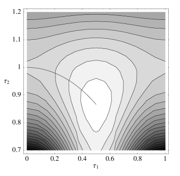
Figure 2: Contour plot of the Casimir potential in the $\tau_{1}$ – $\tau_{2}$ plane. The saddle point where the moduli begin rolling are at $(0,1)$ or $(1,1)$. The minimum is at $(1/2,\sqrt{3}/2)$.

The action for the moduli in an FRW universe has a non-canonical kinetic term:

$$S=\frac{1}{2}M_{Pl}^{2}\int d^{4}x\,\left[a(t)\right]^{3}\left\{\frac{1}{2\tau_{2}^{2}}\left(\dot{\tau_{1}}^{2}+\dot{\tau_{2}}^{2}\right)+V(\tau_{1},\tau_{2})\right\}.$$ (21)

The moduli fields can be defined in terms of the shape parameters:

$$\phi_{1}\equiv\frac{M_{Pl}}{\sqrt{2}}\,\tau_{1},\quad\quad\phi_{2}\equiv\frac{M_{Pl}}{\sqrt{2}}\,\log{\tau_{2}}.$$ (22)

The equation of motion for $\phi_{1}$ (coupled to $\phi_{2}$) is then

$$\ddot{\phi_{1}}+3H\dot{\phi_{1}}-\frac{2\sqrt{2}}{M_{Pl}}\,\dot{\phi_{1}}\dot{\phi_{2}}=\left(-\frac{\partial{V}}{\partial{\phi_{1}}}\right)\,\exp\frac{2\sqrt{2}\,\phi_{2}}{M_{Pl}}.$$ (23)

There is an analogous equation for $\phi_{2}$. Since we are interested in the behavior of the field near the saddle point of the potential, we take $\dot{\phi_{2}}\sim 0$ and the exponential in Eq. (23) to be about one. This can be solved numerically by transforming the coordinates $x\equiv\log{a}=-\log{(1+z)}$ (see [5], for example) which gives an equation of motion:

$$(V+\rho)\,\phi_{1}^{\prime\prime}+3\,(V+\rho)\,\left(1-\phi_{1}^{\prime}{}^{2}/6\right)\phi_{1}^{\prime}+\left(\rho^{\prime}\phi_{1}^{\prime}/2+3\,\partial_{\phi}V\right)\,\left(1-\phi_{1}^{\prime}{}^{2}/6\right)=0.$$ (24)

In the above, $\rho$ is the contribution of matter and radiation to the energy density and a prime indicates a derivative with respect to $x$.

We need to solve Eq. (24) for the time evolution of $\tau_{1}$ given some reasonable “initial” conditions for the field at early redshifts. For this particular form of quintessence the equation of state is almost precisely that of a cosmological constant; that is, $\phi_{1}$ barely rolls over the lifetime of the universe and $w=p/\rho=-1$ to a high accuracy. Thus we simply require that $V_{0}=0.7\rho_{0}$ where $\rho_{0}=1.05\times 10^{-5}h^{2}\,{\rm GeV}\,\mbox{cm}^{-3}$ is the present critical density. The contribution from matter scales as $\rho_{M}=0.3\rho_{0}\,e^{-3x}$ where $x=-\ln(1+z)$. In these variables, big bang nucleosynthesis occurred at $x\approx-20$.

We let the field start near the saddle point at very early redshifts ($z\sim 10^{9}$) with zero initial velocity. The resultant motion is generic and is not sensitive to the initial values specified. In particular, at early times the field is held in place by the large Hubble friction term. Later, as the energy density in the modulus field begins to dominate, the field starts to roll again, providing both quintessence and a change in $\alpha$. Having calculated the evolution of $\tau$ as a function of $z$, we can then calculate the variation of $\alpha$ as a function of $z$, which we do in the next section.

5 Varying Alpha and Constraints

The variation of $\alpha$ as a function of the bulk KK masses was given in Eq. (17) for one extra dimension. This is generalized to:

$$\frac{\alpha_{0}-\alpha(z)}{\alpha_{0}}=\frac{\alpha_{0}}{2\pi}\tilde{b}\sum_{n_{1},n_{2}}^{N}\frac{[{\cal M}_{0}-{\cal M}(z)]_{(n_{1},n_{2})}}{[{\cal M}_{0}]_{(n_{1},n_{2})}}.$$ (25)

where $\alpha_{0}$ and ${\cal M}_{0}$ are present-day values. ${\cal M}$ is implicitly a function of $z$ through its dependence on $\tau_{1}(z)$.

Our ignorance of the fat brane matter content is parameterized by the $\beta$-function coefficient; we assume $\tilde{b}$ is in the range $1\leq\tilde{b}\leq 20$. For models with 2 extra dimensions with sizes in the $\,{\rm meV}^{-1}$ range, the fundamental scale of gravity $M_{*}$ falls in the 10 to $100\,{\rm TeV}$ range. The thickness of the fat brane must be less than roughly $1\,{\rm TeV}^{-1}$ so there is a strict upper bound on the number of KK modes that can lie below the cutoff $M_{*}$. The factor $N$ which cuts off the summation in Eq. (25) parametrizes the number of KK modes allowed and thus the thickness of the fat brane. We assume $N$ is in the range $1\leq N\leq 100$. Because of modular invariance and the need to start near the saddle point, we set $|\tau|=1$ in our numerical work. However we must still choose a value for $\tau_{1}$ at early times; we define $\tau_{0}\equiv\tau_{1}(z=10^{9})$ and vary it near zero.

In Fig. 3 we have plotted $\frac{\delta\alpha}{\alpha}$ (in units of $10^{-5}$) alongside the measurements of Ref. [2] for the several different initial conditions and parameters given in the caption. Note that we define $\delta\alpha(z)=\alpha_{0}-\alpha(z)$. There are a range of initial parameters which fit the data quite well. Each fit has a similar functional behavior, though the amplitude can be quite different. The constraints from big bang nucleosynthesis and WMAP are trivially satisfied because the variation in $\alpha$ is never bigger than it is today – that is, the change in $\alpha$ is a relatively recent phenomenon.

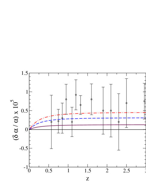
Figure 3: Variation of $\alpha$ for various initial conditions and number of KK modes ($N$) vs. the fiducial sample of Ref. [2]. The solid line corresponds to the values $\tau_{0}=1\times 10^{-5}$, $\tilde{b}=15$, and $N=2$. The dashed line corresponds to the values $\tau_{0}=1\times 10^{-4}$, $\tilde{b}=4$, and $N=8$. The dashed-dot line corresponds to the values $\tau_{0}=1\times 10^{-3}$, $\tilde{b}=1.5$, and $N=3$.

Because the Oklo constraint is of a more recent origin ($z=0.14$), it provides a highly non-trivial constraint on this model. For example, we evaluate the variation in $\alpha$ for the representative examples in the figure. We find:

$$\left\langle\frac{\delta\alpha}{\alpha}\right\rangle_{z=0.14}=(2,6,9)\times 10^{-7}$$ (26)

for the initial conditions shown in the figure. These should be compared with with the $3\,\sigma$ bound $\delta\alpha/\alpha<1.6\times 10^{-7}$ [23]. However more recent work reveals a number of nuclear uncertainties in the calculation of the Oklo bound [24].

A separate constraint arises from measurements of the ¹⁸⁷Re decay rate in the lab and from samples taken from meteorites, which is sensitive to redshifts back to $z\simeq 0.45$. For our three lines, we find:

$$\left\langle\frac{\delta\alpha}{\alpha}\right\rangle_{z=0.45}=(5.8,14,21)\times 10^{-7}$$ (27)

which should be compared with the $3\,\sigma$ bound $\delta\alpha/\alpha<16.0\times 10^{-7}$ [25].

6 Conclusions

A cosmological time variation in the fine structure constant, if verified, presents a difficult theoretical challenge. In this paper we have presented a new mechanism for a late-time variation in a gauge coupling from time-varying charged KK modes. The predicted variation is “soft,” in the sense that only loop effects of charged Kaluza-Klein states contribute to the variation in $\alpha$. This variation does not imply a change in the fundamental Planck scale and relies on the dimensionless shape moduli of the compactification manifold. We have shown that in the case of two large extra dimensions it is possible to interpret both an effective cosmological constant and a varying $\alpha$ in terms of the dynamics of fields sensitive to the shape moduli. In large extra dimensional constructions it is natural that the Standard Model sector has a finite width into the bulk. If the bulk shape moduli are dynamical on cosmological time scales then the Kaluza-Klein mass spectrum of the SM states will be altered. However, this motion typically produces a large change in the vacuum energy; demanding exact supersymmetry above the inverse thickness scale is one possible way of eliminating this potentially dangerous contribution. The only tuning in the model is the initial value of the moduli field at very early redshift. We assume the field starts near a modular invariant of the torus and find that the field begins rolling near redshifts $z\simeq 1$. The post-dicted variation of $\alpha$ is then easily reproduced for reasonable ranges of model parameters.

References

-
[1]
S. Perlmutter et al.,
Ap. J. 517, 565 (1999);
A. G. Riess et al., Astron. J. 116, 1009 (1998);
D. N. Spergel et al., Ap. J. Suppl. 148, 175 (2003). -
[2]
J. K. Webb et al.,
Phys. Rev. Lett. 82, 884 (1999);
M. T. Murphy, J. K. Webb, and V. V. Flambaum, Mon. Not. Roy. Astron. Soc. 345, 609 (2003). -
[3]
J. N. Bahcall, C. L. Steinhardt and D. Schlegel,
Ap. J. 600, 520 (2004);
T. Ashenfelter, G. J. Mathews, and K. A. Olive, Phys. Rev. Lett. 92, 041102 (2004). -
[4]
G. R. Dvali and M. Zaldarriaga,
Phys. Rev. Lett. 88, 091303 (2002);
T. Chiba and K. Kohri, Prog. Theor. Phys. 107, 631 (2002);
E. J. Copeland, N. J. Nunes and M. Pospelov, Phys. Rev. D 69, 023501 (2004). - [5] L. Anchordoqui and H. Goldberg, Phys. Rev. D 68, 083513 (2003).
- [6] S. M. Carroll, Phys. Rev. Lett. 81, 3067 (1998).
- [7] C. F. Kolda and D. H. Lyth, Phys. Lett. B 458, 197 (1999).
- [8] M. Peloso and E. Poppitz, Phys. Rev. D 68, 125009 (2003).
- [9] M. Pietroni, Phys. Rev. D 67, 103523 (2003).
- [10] Z. Chacko, C. Grojean, M. Perelstein, Phys. Lett. B 565, 169 (2003).
- [11] K. R. Dienes, Phys. Rev. Lett. 88, 011601 (2002).
- [12] T. Appelquist, H.-C. Cheng, B. A. Dobrescu, Phys. Rev. D 64, 035002 (2001).
- [13] R. Sundrum, Phys. Rev. D 59, 085009 (1999).
- [14] N. Arkani-Hamed, S. Dimopoulos and G. R. Dvali, Phys. Rev. D 59, 086004 (1999).
-
[15]
J. C. Long and J. C. Price,
Comptes Rendus Physique 4, 337 (2003);
E. G. Adelberger, B. R. Heckel and A. E. Nelson, arXiv:hep-ph/0307284. - [16] S. Cullen and M. Perelstein, Phys. Rev. Lett. 83, 268 (1999).
- [17] M. Byrne and P. Regan, in preparation.
- [18] A. De Rujula, A. Donini, M. B. Gavela and S. Rigolin, Phys. Lett. B 482, 195 (2000).
- [19] C. Macesanu, A. Mitov and S. Nandi, Phys. Rev. D 68, 084008 (2003).
- [20] R. S. Chivukula, D. A. Dicus, H. J. He and S. Nandi, Phys. Lett. B 562, 109 (2003).
-
[21]
T. Banks, M. Dine, M. R. Douglas,
Phys. Rev. Lett. 88, 131301 (2002);
P. Langacker, G. Segre, M. J. Strassler, Phys. Lett. B 528, 121 (2002). - [22] E. Ponton and E. Poppitz, JHEP 0106, 019 (2001).
- [23] T. Damour and F. Dyson, Nucl. Phys. B 480, 37 (1996).
- [24] S. K. Lamoreaux, arXiv:nucl-th/0309048.
- [25] K. A. Olive, M. Pospelov, Y. Z. Qian, G. Manhes, E. Vangioni-Flam, A. Coc and M. Casse, Phys. Rev. D 69, 027701 (2004).