Abstract

It is shown that hypothetical neutrino-majoron coupling can suppress neutrino flavor oscillations in the early universe, in contrast to the usual weak interaction case. This reopens a window for a noticeable cosmological lepton asymmetry which is forbidden for the large mixing angle solution in the case of standard interactions of neutrinos.

1 Introduction

Cosmological lepton asymmetry is not directly measurable, in contrast to baryon asymmetry, but may be observed or restricted through its impact on big bang nucleosynthesis (BBN), large scale structure formation, and the angular spectrum of the cosmic microwave background radiation (CMBR), for a review see e.g. Ref. [1]. At the present time the best bounds follow from the consideration of BBN. Primordial production of light elements is especially sensitive to the value of asymmetry between electronic neutrinos and antineutrinos since they directly influence the neutron-proton transformations in weak reactions $\nu_{e}\,n\leftrightarrow e^{-}p$ and $\bar{\nu}_{e}\,p\leftrightarrow e^{+}n$. The bound on the chemical potential of electronic neutrinos obtained in Ref. [2] reads $|\xi_{e}|\equiv|\mu_{e}/T|<0.1$. The bound on muonic or tauonic asymmetry is noticeably weaker because $\nu_{\mu}$ or $\nu_{\tau}$ produce an effect on BBN only through their impact on the cooling rate of the universe and the degeneracy of these neutrino flavors is equivalent to an addition of

$$\Delta N_{\nu}=\frac{15}{7}\,\left[\left(\frac{\xi_{\mu,\tau}}{\pi}\right)^{4}+2\,\left(\frac{\xi_{\mu,\tau}}{\pi}\right)^{2}\right]$$ (1)

massless neutrino species at the BBN epoch. If the latter is bounded by $\Delta N_{\nu}<1$ (safe bound) then $|\xi_{\mu,\tau}|<1.5$. For less conservative bound, $\Delta N_{\nu}<0.4$ [3], the dimensionless chemical potentials should be below 0.9. Still, asymmetry of the order of unity would have noticeable cosmological effects on large scale structure formation and CMBR. The limits quoted above are valid if the chemical potential of only one kind of neutrino is non-zero. If a conspiracy between different chemical potentials is allowed, such that a positive effect of $\xi_{\mu}$ or $\xi_{\tau}$ is compensated by $\xi_{e}$ or vice versa, the limits would be somewhat weaker. According to Ref. [4] they are: $|\xi_{e}|<0.2$ and $|\xi_{\mu,\tau}|<2.6$.

The bounds on chemical potentials of $\nu_{\mu}$ and $\nu_{\tau}$ can be significantly improved because of the strong mixing between different neutrino flavors [6]. This mixing gives rise to the fast transformation between $\nu_{e}$, $\nu_{\mu}$, and $\nu_{\tau}$ in the early universe and leads to equilibration of asymmetries of all neutrino species. Thus the BBN bound on any chemical potential becomes essentially that obtained for $\nu_{e}$ [7] (see also the papers [8]):

$$|\xi_{e,\mu,\tau}|<0.07.$$ (2)

In this case the cosmological impact of neutrino degeneracy would be negligible. However, a compensation of $\xi_{e}$ by other types of radiation is still possible, which was studied in Ref. [9]. The authors of Ref. [9] put the constraints on $\xi_{e}$ and $\Delta N_{\nu}$ based on WMAP data and BBN:

$$-0.1\mathop{}_{\textstyle\sim}^{\textstyle<}\xi_{e}\mathop{}_{\textstyle\sim}^{\textstyle<}0.3,~{}~{}-2\mathop{}_{\textstyle\sim}^{\textstyle<}\Delta N_{\nu}\mathop{}_{\textstyle\sim}^{\textstyle<}5.$$ (3)

It is interesting to see if one could reasonably modify the standard model to allow large muonic and/or tauonic charge asymmetries, together with a small electronic asymmetry, to avoid conflict with BBN. This is the aim of this work. A natural generalization is to introduce an additional interaction of neutrinos with massless or light (pseudo)Nambu-Goldstone boson, majoron [10]. The idea to invoke majoron to modify neutrino oscillations in primeval plasma was discussed in Refs. [11, 12]. In these papers, two different mechanisms which could block or suppress oscillations between active and hypothetical sterile neutrinos have been considered. We have, however, some concerns about the validity of their results which we will discuss in the next section. Let us note that in this paper we consider an impact of neutrino majoron interactions on the oscillations between active neutrinos and not on active-sterile oscillations, as is done in the mentioned above papers.

2 General discussion and approximate estimates

Neutrino oscillations may be suppressed in medium if the interaction of neutrinos with the medium is sufficiently strong or in other words the refraction index, $n$ (or effective potential, $V=E(n-1)$) of neutrinos is very large. Correspondingly the mixing angle in medium $\theta_{m}$ becomes negligible:

$$\tan^{2}2\theta_{m}={s_{2}^{2}\over\left(c_{2}^{2}+V/\delta E\right)^{2}+\Gamma^{2}/(4\delta E^{2})}$$ (4)

where $s_{2}=\sin 2\theta$, $c_{2}=\cos 2\theta$, $\theta$ is the vacuum mixing angle, $\delta E={\delta m^{2}}/2E$, $E$ is the neutrino energy, and $\Gamma$ is the rate of neutrino interaction with medium given by

$$\Gamma=\frac{80(1+g_{L}^{2}+g_{R}^{2})\,G^{2}_{F}ET^{4}}{3\pi^{3}}$$ (5)

where $T$ is the temperature of the primeval plasma, $G_{F}=1.166\cdot 10^{-11}\,{\rm MeV}^{-2}$ is the Fermi coupling constant, $g_{L}=\sin^{2}\theta_{W}\pm 1/2$ and $g_{R}=\sin^{2}\theta_{W}$ where $\sin^{2}\theta_{W}=0.23$ and the sign ${}^{\prime\prime}+^{\prime\prime}$ stands for $\nu_{e}$ and ${}^{\prime\prime}-^{\prime\prime}$ stands for $\nu_{\mu,\tau}$. The derivation of these equations can be found e.g. in lectures [13].

The diagonal components of the effective potential, created by the standard weak interaction, for the active neutrino species are given by [14]:

$$V_{aa}^{(w)}=\pm C_{1}\eta^{(a)}G_{F}T^{3}-C_{2}^{a}\frac{G^{2}_{F}T^{4}E}{\alpha}$$ (6)

where $a=e,\mu,\tau$ labels the neutrino flavors, $\alpha=1/137$ is the fine structure constant, and the signs “$\pm$” refer to neutrinos and antineutrinos respectively. The first term arises due to a possible charge asymmetry of the primeval plasma, while the second one comes from the non-locality of weak interactions associated with the exchange of $W$ or $Z$ bosons. According to Ref. [14] the coefficients $C_{j}$ are: $C_{1}\approx 0.95$, $C_{2}^{e}\approx 0.62$ and $C_{2}^{\mu,\tau}\approx 0.17$ (for $T<m_{\mu}$). These values are true in the limit of thermal equilibrium, otherwise these coefficients are some integrals from the distribution functions over momenta. The charge asymmetry of plasma is described by the coefficients $\eta^{(a)}$ which are equal to

$$\eta^{(e)} = 2\eta_{\nu_{e}}+\eta_{\nu_{\mu}}+\eta_{\nu_{\tau}}+\eta_{e}-\eta_{n}/2\,\,\,({\rm for}\,\,\nu_{e})~{},$$ (7)

$$\eta^{(\mu)} = 2\eta_{\nu_{\mu}}+\eta_{\nu_{e}}+\eta_{\nu_{\tau}}-\eta_{n}/2\,\,\,({\rm for}\,\,\nu_{\mu})~{},$$ (8)

and $\eta^{(\tau)}$ for $\nu_{\tau}$ is obtained from Eq. (8) by the interchange $\mu\leftrightarrow\tau$. The individual charge asymmetries, $\eta_{X}$, are defined as the ratio of the difference between particle-antiparticle number densities to the number density of photons with the account of the 11/4-factor emerging from the $e^{+}e^{-}$-annihilation:

$$\eta_{X}=\left(N_{X}-N_{\bar{X}}\right)/N_{\gamma}.$$ (9)

For “normal” values of charge asymmetry, i.e. $|\eta|\sim 10^{-9}$ the charge asymmetric term in the potential (6) is subdominant but if the asymmetry is of the order of unity, then the ratio $V_{aa}/{\delta E}$ becomes huge:

$$V_{aa}^{(w)}/{\delta E}\approx 2\cdot 10^{-11}\eta ET^{3}({\delta m^{2}})^{-1}\left({\rm MeV}\right)^{-2}\approx 20\eta\left(T/{\rm MeV}\right)^{4}({\rm eV}^{2}/{\delta m^{2}})$$ (10)

and e.g. for ${\delta m^{2}}=10^{-2}$ eV² and $\eta\sim 1$ the mixing angle in matter would be suppressed more than by three orders of magnitude in the BBN range of temperatures, $T\sim$MeV.

However, this result is valid for mixing between active and sterile neutrinos and is not true for active-active mixing. In the last case the effective potential has large off-diagonal matrix elements [15], $V_{ab}$, with $a\neq b$, which compensate the suppression induced by the diagonal terms. This is the reason for non-suppressed oscillations between active flavors and for the equilibration of all leptonic asymmetries [7].

Possible additional interactions of neutrinos with majoron can be described by the Lagrangian:

$${\cal L}_{int}\sim\chi(g_{ab}\nu_{a}^{T}C\nu_{b}+h.c)$$ (11)

where $\chi$ is the operator of the majoron field, $C$ is the matrix of charge conjugation, and $g_{ab}$ are the coupling constants. We will assume for simplicity, though it is not necessary, that only the flavor-diagonal coupling is non-vanishing, $g_{ab}\sim g_{aa}\delta_{ab}$. We will consider the coupling matrix with more general form later. Let us also assume that the majoron is so light that its decay and inverse decay are not essential at the BBN epoch. Neutrino-(anti)neutrino scattering through majoron exchange gives rise to a contribution to neutrino effective potential (proportional to forward scattering amplitude) which can be estimated as

$$V^{(\chi)}_{ab}\sim g_{aa}g_{bb}T.$$ (12)

The constants $g_{aa}$ should satisfy several constraints to make the mechanism operative. Firstly, the diagonal part of the potential $V^{(\chi)}_{aa}$ should be larger than the weak potential $V^{(w)}$ given by Eq. (6), while its off-diagonal components must be much smaller than the diagonal ones, $V^{(\chi)}_{ab}<<V^{(\chi)}_{aa}$, that is, the flavor symmetry in the neutrino-majoron interactions should be strongly broken. These two conditions would ensure suppression of flavor changing oscillations between active neutrinos. To realize these conditions the following constraints should be imposed:

$$g_{aa}^{2}>10^{-11}\eta^{(a)}\,\left(\frac{T_{ae}}{1{\rm~{}MeV}}\right)^{2}\,\,\,{\rm and}\,\,\,g_{ee}\ll g_{aa}.$$ (13)

Here $a$ labels $\mu$ or $\tau$ and the coupling of majoron to $\nu_{e}$ is assumed to be much weaker than those to $\nu_{\mu}$ and/or $\nu_{\tau}$; $T_{ae}$ is the temperature at which $\nu_{a}$ are effectively transformed into $\nu_{e}$ in the standard theory. According to calculations of Ref. [7] it takes place around $T_{ae}=1$ MeV for the large mixing angle solution to solar neutrino deficit, while the transformation between $\nu_{\mu}$ and $\nu_{\tau}$ in the standard theory takes place somewhat above 10 MeV. In fact, as we see in what follows from numerical calculations, the more accurate bound is much less restrictive than this simple estimate (see Eq. (49) or Figs. 6 and 7 below).

The second inequality (13) implies that the off-diagonal components of the effective potential are suppressed in comparison with the diagonal ones and the oscillations remain blocked. This is not so in the case of the standard weak interactions which are flavor symmetric and the large value of the denominator due to large $V_{aa}$ in Eq. (4) is compensated by the same large off-diagonal components of the effective potential.

Secondly, the coupling constants $g_{aa}$ should not be too large, otherwise flavor non-conserving reactions of the type $\nu_{e}\,\nu_{a}\leftrightarrow\bar{\nu}_{e}\bar{\nu}_{a}$ (or similar) would lead to equilibration of all leptonic charges. To avoid that the rate of these reactions, $\Gamma_{ea}\sim\sigma_{ea}T^{3}$, should be smaller than the cosmological expansion rate $H\sim T^{2}/m_{Pl}$, where $m_{Pl}=1.221\cdot 10^{22}$ MeV is the Planck mass. Thus, to suppress $e-\mu$ or $e-\tau$ transformation through direct reactions one needs

$$g_{aa}^{2}g_{ee}^{2}<10^{-22}\left(\frac{T}{1{\rm~{}MeV}}\right).$$ (14)

This conditions should be satisfied for temperatures above the BBN range, i.e. $T>1$ MeV. Similarly, if we require that $\nu_{a}\,\nu_{a}\leftrightarrow\bar{\nu}_{a}\bar{\nu}_{a}$ should not occur efficiently, the coupling constants must satisfy a similar inequality with $g_{ee}$ replaced with $g_{aa}$.

There are quite strong limits on possible coupling of majoron to neutrinos which follow from astrophysics [16, 17]; discussion and references to earlier works can be found e.g. in the book [18]. Astrophysics allows either very small or quite large coupling constants. The former is quite evident, while the latter appears because strongly interacting majorons, though efficiently produced inside a star, cannot propagate out and carry away the energy, thus opening a window for large values of the coupling. It is not so for the coupling to $\nu_{e}$ because the latter is bounded from above by the data on double beta decay [19], $g_{ee}<3\cdot 10^{-5}$. Together with the supernova bounds, the upper limit is shifted down to $g_{ee}<4\cdot 10^{-7}$ [17], with a small window around $(2-3)\cdot 10^{-5}$. So we assume in the following that $g_{ee}<4\cdot 10^{-7}$. For $\mu$ or $\tau$ the allowed regions are: $g_{aa}<(3-5)\cdot 10^{-6}$ or $g_{aa}>(3-5)\cdot 10^{-5}$. Evidently the conditions specified above can be satisfied. As reference values we may take $g_{ee}=10^{-7}$ and $g_{aa}=5\cdot 10^{-6}$ which satisfy all constraints presented above and would lead to a suppression of the transformation of $\nu_{\mu}$ or $\nu_{\tau}$ into $\nu_{e}$, thus permitting a large muonic or tauonic asymmetry combined with a small electronic one at BBN. Note that it is not necessary to assume a large value of $g_{aa}\mathop{}_{\textstyle\sim}^{\textstyle>}10^{-5}$ to accomplish this. As shown later, such a large coupling constant would change the scenario into something more complex.

If majoron is lighter than the mass difference of neutrinos then a heavier neutrino would decay into a lighter one and majoron. This process might leave traces in the flavor ratios of the high-energy neutrinos from distant astrophysical sources [20], which can be detected by e.g., IceCube [21]. This could be potentially sensitive to very small values of the neutrino-majoron coupling. Existing bound [22] on life-time/mass of decaying neutrinos based on the solar neutrino data, $\tau/m\geq 10^{-4}$ sec/eV, is too weak to be essential for the mechanism discussed in the present paper.

In the subsequent sections we will present more accurate calculations but before turning to a closer examination of the scenario, let us make a few comments on earlier papers where majoron suppression of neutrino oscillations in the early universe have been considered. In Ref. [11] it was assumed that there exists a coupling of an active and sterile neutrinos to majoron. Let us note that in the version of the theory that we consider here no sterile neutrinos are introduced: the negative helicity states are identified with neutrinos, while the positive helicity states are identified with antineutrinos. The coupling considered in Ref. [11] has the form:

$${\cal L}_{as}=ig_{as}\,\chi\bar{\nu}_{a}\nu_{s}+h.c.$$ (15)

where $\nu_{a}$ is an active neutrino flavor and $\nu_{s}$ is a sterile one. The authors argued that the effective potential induced by the interactions of active and sterile neutrinos with majoron strongly suppressed the oscillations. However they omitted off-diagonal $V_{as}$-term in the effective potential which might invalidate their result. Possibly this mechanism of oscillation suppression may operate in a more complicated version of the model.

In Ref. [12] a different mechanism of neutrino oscillation blocking by majoron has been suggested. According to the equation of motion, the total leptonic current including majoron and neutrino contributions is conserved:

$$fD^{2}\chi+D_{\mu}J^{\mu}=0$$ (16)

where $D_{\mu}$ is the covariant derivative in cosmological background, $f$ is the vacuum expectation value of the Higgs field responsible for the spontaneous breaking of leptonic $U_{L}(1)$-symmetry and $J^{\mu}$ is the leptonic currents of fermions. In spatially homogeneous case the solution to this equation is

$$\dot{\chi}(t)=\left[\frac{a_{in}}{a(t)}\right]^{3}\,\left(\dot{\chi}_{in}-J_{in}^{t}/f\right)+J^{t}(t)/f,$$ (17)

where $a(t)$ is the cosmological scale factor and the sub-index “in” indicates initial values. We assume that $\dot{\chi}_{in}=0$. Hence the authors of Ref. [12] concluded that $\dot{\chi}=\eta_{B}n_{\gamma}/f$, where $\eta_{B}=6\cdot 10^{-10}$ is the baryon asymmetry of the universe. The contribution to the neutrino effective potential from this term is $\delta V^{\chi}=\dot{\chi}/f$ and, according to [12], with $f^{2}=(5-9)$ GeV² the potential would be strong enough to suppress the oscillations. However, according to the usual scenarios, baryon asymmetry could be created at much larger temperatures, much higher than this scale. Thus, after spontaneous symmetry breaking, leading to creation of majoron, $J^{t}$ remains constant in comoving volume and $\dot{\chi}=0$. A non-zero $\dot{\chi}$ might be created if lepton asymmetry was generated at spontaneous breaking of leptonic $U_{L}(1)$ or by the neutrino oscillations themselves but both these cases need further and more detailed investigation. So in our considerations we assume that the mechanism of Ref. [12] is not operative.

3 Effective potential induced by neutrino-majoron interactions

In this section we derive the effective potential induced by the neutrino-majoron interactions, which is one of essential ingredients of our paper. The relevant part of the Lagrangian is given by

$${\cal L} = -\frac{1}{2}\partial_{\mu}\chi\partial^{\mu}\chi-\sum_{a}\overline{\nu}_{a}\gamma^{\mu}\partial_{\mu}\nu_{a}+{\cal L}_{int},$$ (18)

$${\cal L}_{int} = \frac{1}{2}\chi\left(g_{ab}\,\Phi_{a}^{T}\sigma_{2}\Phi_{b}+g_{ab}^{*}\,\Phi_{b}^{\dagger}\sigma_{2}\Phi_{a}^{*}\right),$$ (19)

$$= \frac{i}{2}\chi\left(g_{ab}\,\nu_{a}^{T}C\nu_{b}+g_{ab}^{*}\,\nu_{b}^{\dagger}C\nu_{a}^{*}\right),$$

where $\Phi_{a}$ and $\nu_{a}$ are two-component and four-component representations of neutrino of flavor $a$, respectively. They are related to each other as $\nu_{a}^{T}=(\Phi_{a}^{T},0)^{T}$ in the chiral representation (see Appendix A for notations). Here and hereafter $\nu_{a}$ is taken to be the left-handed field. In the following we neglect the effect of small masses of neutrinos, and treat them as massless fields. In this limit, there are three diagrams that contribute to the effective potential (see Figs. 1 and 2 ).

Let us first calculate the effective Hamiltonian corresponding to neutrino-(anti)neutrino scattering processes. For that purpose we integrate out the majoron field using its equation of motion, and substitute the solution into interaction Lagrangian (19). Then we quantize neutrino fields perturbatively. The details of the derivation can be found in the Appendix A. The effective Hamiltonian, which describes the neutrino-(anti)neutrino scattering processes, is given by

$${\cal H}_{\rm eff}^{(\nu\nu)}(t)=-\frac{(2\pi)^{3}}{16}\int d{\bf p}\,d{\bf q}\,d{\bf r}\,d{\bf s}\,\,\frac{\delta^{(3)}({\bf p+q+r+s})\,e^{-iE_{\rm tot}t}F({\bf p},{\bf q})F({\bf r},{\bf s})}{\epsilon_{p}\epsilon_{q}E_{\bf p}E_{\bf q}(1-\epsilon_{p}\epsilon_{q}\cos\theta_{\bf pq})}$$ (20)

with

$$E_{\bf p} \equiv \left|{\bf p}\right|,$$

$$E_{\rm tot} \equiv \epsilon_{p}E_{\bf p}+\epsilon_{q}E_{\bf q}+\epsilon_{r}E_{\bf r}+\epsilon_{s}E_{\bf s},$$

$$\cos\theta_{\bf pq} \equiv \frac{{\bf p}\cdot{\bf q}}{\left|{\bf p}\right|\left|{\bf q}\right|},$$

$$F({\bf p},{\bf q}) \equiv g_{ab}\,\nu_{a}({\bf p})^{T}C\nu_{b}({\bf q})+g_{ab}^{*}\,\nu_{b}({\bf-q})^{\dagger}C\nu_{a}^{*}({\bf-p}),$$ (21)

where $d{\bf p}\equiv d^{3}{\bf p}/(2\pi)^{3}$. The momentum expansion of free neutrino field is

$$\nu_{i}(x) = \int d{\bf p}~{}\nu_{i}({\bf p})\,e^{-ip^{0}t+i{\bf p}\,{\bf x}},$$ (22)

$$= \int d{\bf p}~{}\left(a_{i}({\bf p})u_{\bf p}+b_{i}({\bf-p})^{\dagger}v_{\bf-p}\right)\,e^{-ip^{0}t+i{\bf p}\,{\bf x}}$$

with $p^{0}\equiv\epsilon_{p}\left|{\bf p}\right|=\pm\left|{\bf p}\right|$. The sign of $\epsilon_{p}$ is chosen to reproduce positive or negative energy solution. Here $a_{i}({\bf p})$ ($b_{i}{}^{\dagger}({\bf p})$) is the annihilation (creation) operator for negative (positive)-helicity neutrinos with momentum ${\bf p}$, $u_{\bf p}$($v_{\bf p}$) represents left-handed Dirac spinor of negative (positive)-helicity neutrinos. With thus obtained effective Hamiltonian, the effective potential can be calculated by the technique of Sigl and Raffelt [23]. Although the calculations are lengthy, the procedure is straightforward. The contribution to the effective potential for neutrinos with momentum ${\bf p}$ is given by

$$\left[V_{\bf p}^{(\nu\nu)}\right]_{ab}=\int d{\bf q}~{}~{}\frac{1}{4\left|{\bf p}\right|\left|{\bf q}\right|}\left[g^{\dagger}\left(\rho^{T}_{\bf q}+\overline{\rho}^{T}_{\bf q}\right)g\right]_{ab},$$ (23)

where the density matrices are defined as

$$\left\langle a^{\dagger}_{j}({\bf p})\,a_{i}({\bf p}^{\prime})\right\rangle = (2\pi)^{3}\delta^{(3)}({\bf p}-{\bf p}^{\prime})\left[\rho_{\bf p}\right]_{ij},$$

$$\left\langle b^{\dagger}_{i}({\bf p})\,b_{j}({\bf p}^{\prime})\right\rangle = (2\pi)^{3}\delta^{(3)}({\bf p}-{\bf p}^{\prime})\left[\overline{\rho}_{\bf p}\right]_{ij}.$$ (24)

If we take the coupling constant matrix $g_{ab}$ to be diagonal, the effective potential becomes

$$\left[V_{\bf p}^{(\nu\nu)}\right]_{ab} = g^{*}_{aa}g_{bb}\int d{\bf q}~{}~{}\frac{1}{4\left|{\bf p}\right|\left|{\bf q}\right|}\left(\rho^{T}_{\bf q}+\overline{\rho}^{T}_{\bf q}\right)_{ab}~{}~{}~{}(\rm{no~{}summation}),$$

$$\sim g^{*}_{aa}g_{bb}\frac{T^{2}}{\left|{\bf p}\right|}.$$

This result confirms the rough estimate of the effective potential in the previous section.

The neutrino-majoron scattering shown in Fig. 2 also contributes to the effective potential and can be calculated similarly. The result is

$$\left[V_{\bf p}^{(\nu\chi)}\right]_{ab}=\int d{\bf q}~{}~{}\frac{f_{\chi}({\bf q})}{4\left|{\bf p}\right|\left|{\bf q}\right|}\left[g^{\dagger}g\right]_{ab},$$ (25)

where $f_{\chi}({\bf p})$ is the number density of majorons with momentum $\bf{p}$. Note that this expression vanishes if the abundance of majorons is negligible in comparison with their equilibrium value, i.e. $f_{\chi}({\bf p})\ll f_{\chi}^{(eq)}({\bf{p}})$. Thus the complete effective potential for neutrinos with momentum ${\bf p}$ induced by interactions with majorons is given by

$$\left[V_{\bf p}^{(\chi)}\right]_{ab}=\int d{\bf q}~{}~{}\frac{1}{4\left|{\bf p}\right|\left|{\bf q}\right|}\left[g^{\dagger}\left(\rho^{T}_{\bf q}+\overline{\rho}^{T}_{\bf q}+f_{\chi}({\bf q})\cdot{\bf 1}\right)g\right]_{ab},$$ (26)

where ${\bf 1}$ is the unit matrix in the flavor basis.

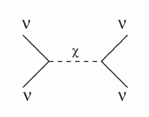
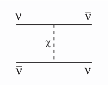
Figure 1: s- and t-channel diagrams of neutrino-(anti)neutrino scattering through majoron exchange. Both diagrams contribute to the off-diagonal component of the effective potential.

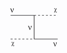
Figure 2: Diagram of neutrino-majoron scattering through neutrino exchange. If majorons are not abundant in the primeval plasma, this diagram gives negligible contribution to the effective potential.

4 Possible role of neutrino-majoron reactions.

As we have already mentioned reactions between neutrinos with an exchange of majorons do not conserve leptonic charge and if they are efficient, lepton asymmetry of the universe would be completely destroyed before BBN. One of the dangerous processes is

$$2\nu\leftrightarrow 2\bar{\nu}.$$ (27)

We assume for simplicity that the diagonal coupling constants $|g_{aa}|$ are larger than non-diagonal ones and that one flavor coupling dominates, e.g. $|g_{\tau\tau}|>|g_{\mu\mu}|>|g_{ee}|$. In this case only three diagrams presented in Fig. 3 contribute into the reaction (27). The amplitude corresponding to any of these three diagram is equal to $|g|^{2}$ and thus the complete amplitude squared is simply $|A(2\nu\leftrightarrow 2\bar{\nu})|^{2}=9|g|^{4}$ (see Appendix B). Here and in what follows we omit the sub-index $aa$ at the coupling constant $g_{aa}$. With the known amplitude of the $L$-nonconserving reaction ($L$ is the leptonic charge), the kinetic equation can be written as

$$\frac{h}{x^{2}}\,x\,\partial_{x}f_{\bar{\nu}}(y_{1})=\frac{1}{2}\cdot\frac{9|g|^{4}}{2^{9}\pi^{5}xy_{1}}\int\frac{d^{3}\bf{y}_{2}}{y_{2}}\frac{d^{3}{\bf y}_{3}}{y_{3}}\frac{d^{3}{\bf y}_{4}}{y_{4}}\,F(f)\,\delta^{(4)}(y_{1}+y_{2}-y_{3}-y_{4})+I_{coll}^{(el)}$$ (28)

where $f$ is the neutrino distribution function, $(y_{i},{\bf y}_{i})=(E_{i}/T,{\bf p}_{i}/T)$, $x=(T/{\rm MeV})^{-1}$, $T$ is the temperature of the cosmic plasma, $(H/{\rm MeV})=h/x^{2}$ is the Hubble parameter with $h\approx 4.5\cdot 10^{-22}$, $I_{coll}^{(el)}$ is the contribution to the collision integral from reactions that conserve leptonic charge, and

$$F(f)=[1-f_{\bar{\nu}}(y_{1})][1-f_{\bar{\nu}}(y_{2})]f_{\nu}(y_{3})f_{\nu}(y_{4})-[1-f_{\nu}(y_{3})][1-f_{\nu}(y_{4})]f_{\bar{\nu}}(y_{1})f_{\bar{\nu}}(y_{2}).$$ (29)

We assumed that the temperature evolved according to $\dot{T}=-HT$. The combinatorial factor $1/2$ in front of the r.h.s. comes from two factors $1/2!$ and one factor 2 because two identical particle are produced (see e.g. Ref. [24]).

The collision integral in Eq. (28) can be easily evaluated in the limit of Boltzmann statistics, when $f\ll 1$ and under assumption of kinetic equilibrium, so the distribution functions have the form $f=\exp(-y+\xi)$, where $\xi=\mu/T$ is the dimensionless chemical potential. To avoid the contribution of $I_{coll}^{(el)}$ to the equation governing the evolution of $\xi$ we take the difference of Eq. (28) and analogous equation for $f_{\nu}$ and integrate it over $d^{3}{\bf y}_{1}$. The contribution of $I_{coll}^{(el)}$ to this integrated difference vanishes. The resulting equation takes the form:

$$\partial_{x}\left(e^{\xi}-e^{\bar{\xi}}\right)=-\frac{9|g|^{4}}{2^{7}\pi^{3}h}\left(e^{2\xi}-e^{2\bar{\xi}}\right),$$ (30)

where we have used the formula presented in Appendix C. It is also assumed above that $\xi=-\bar{\xi}$. Otherwise the contribution from $L$-conserving $\bar{\nu}\nu$-annihilation would not vanish in the collision integral. If $\xi\geq 1$ we may neglect $\exp(-\xi)$ and solve equation (30) as

$$\exp[\xi(x)]=\frac{\exp[\xi(0)]}{1+9|g|^{4}x\exp[\xi(0)]/(128\pi^{3}h)}$$ (31)

The lepton asymmetry would not be destroyed by reaction (27) if

$$|g|<2\cdot 10^{-5}T^{1/4}\exp[-\xi(0)/4].$$ (32)

Here (and in what follows) $T$ is given in MeV. Quantum statistics (Fermi) effects somewhat weaken the bound. Their presence does not allow to solve kinetic equation analytically. Numerical estimates give a similar constraint as shown in Fig. 5.

Muonic or tauonic charge asymmetry should be preserved until the annihilation $\bar{\nu}_{\tau,\mu}\nu_{\tau,\mu}$ into $e^{+}e^{-}$-pairs is frozen. Otherwise we will return to the standard scenario with zero lepton asymmetry. According to the estimates of Ref. [13] made in Boltzmann approximation, the freezing temperature of the annihilation is $T_{f}\approx 5.3$ MeV. Fermi corrections would make its value slightly higher. If muonic and/or tauonic charge asymmetry were erased by the oscillations or L-nonconserving reactions with exchange of majorons below $T_{f}$ then the total number density of $\nu_{\tau}$ plus $\bar{\nu}_{\tau}$ (or $\nu_{\mu}+\bar{\nu}_{\mu}$) would be conserved in the comoving volume and their distribution would be given by

$$f_{\nu_{a}}=f_{\bar{\nu}_{a}}=\left[\exp(E/T-\xi_{a})\right]^{-1}$$ (33)

where $a=\mu,\tau$. So effectively the energy density of these neutrinos would be the same (up to a numerical factor of order of unity) as the energy density of the usual degenerate neutrinos. If the mixing of $\nu_{\tau}$ or $\nu_{\mu}$ with $\nu_{e}$ would not change the distribution of the latter then BBN would allow a large values of $\xi_{a}$ and the degeneracy of $\nu_{a}$ may lead to noticeable cosmological effects.

We make a simplifying assumption of absence of majorons in noticeable amount in the primeval plasma. If majorons would be in equilibrium we should take into account their (4/7)-contribution into the number of effective neutrino species at BBN and modification of neutrino effective potential due to forward elastic scattering $\nu\chi\rightarrow\nu\chi$. Even if majorons are abundantly produced, the main conclusion of our paper remains unchanged but numerical results would be somewhat different. The production of majorons could proceed through the reaction $\nu+\bar{\nu}\rightarrow 2\chi$. The Feynman diagrams describing this process are presented in Fig. 4. The amplitude squared of this process is

$$\left|M_{\rm inv}\right|^{2}=|g|^{4}\left(\frac{p_{1}\cdot p_{3}}{p_{1}\cdot p_{4}}+\frac{p_{1}\cdot p_{4}}{p_{1}\cdot p_{3}}-2\right),$$

where $p_{1(2)}$ and $p_{3,4}$ are four momenta for (anti)neutrino in the initial state and majorons in the final state, and they satisfy the momentum conservation condition, $p_{1}+p_{2}=p_{3}+p_{4}$. Note that the collision integral with this amplitude squared involves an IR logarithmic divergence, therefore we need to input a lower cutoff scale. Taking into account the thermal effects, the dispersion relations for the majoron and the neutrinos change from those at zero temperature. Especially, they obtain finite thermal masses, which provide the desired infra-red cutoff. For $|g|\sim O(10^{-5})$, the thermal effect of the neutrino-majoron interaction dominates over that due to the electroweak interaction, so the IR divergent part is regularized as $\sim\log(4E^{2}/m_{T}^{2})$ with $m_{T}\sim|g|T$.

Kinetic equation governing the production of majorons is similar to Eq. (28), and has the form:

$$\frac{h}{x^{2}}x\partial_{x}f_{\chi}=\frac{|g|^{4}\log(4E^{2}/m_{T}^{2})}{2^{7}\pi^{3}x}\,\frac{\exp(-y)}{y}+...$$ (34)

where we omitted elastic reactions. Integrating this equation we can find for the ratio of the number density of $\chi$ to the equilibrium value:

$$\frac{n_{\chi}}{n_{\chi}^{(eq)}}=\frac{|g|^{4}\log(4E^{2}/m_{T}^{2})~{}x}{2^{8}\zeta(3)\pi^{3}h}$$ (35)

Demanding that $n_{\chi}<n_{\chi}^{(eq)}$ we obtain

$$|g|<2.1\cdot 10^{-5}T^{1/4},$$ (36)

which gives a constra int similar to Eq. (32). However, if we take into account quantum statistics, the bound becomes slightly weaker for large charge asymmetry of neutrinos, as shown in Fig. 5.

So, to summarize, the muonic or tauonic lepton asymmetry would be erased if the neutrino-majoron interaction is sufficiently strong, i.e. $|g|\mathop{}_{\textstyle\sim}^{\textstyle>}10^{-5}$. If we restrict ourselves to a scenario that the majoron-neutrino interactions suppress neutrino oscillations and thereby keep the large lepton asymmetries intact, the largest coupling constant should be smaller than $\sim 10^{-5}$. However this does not necessarily mean that the conspiracy between the speed-up effect of $\xi_{\mu,\tau}$ and a shift of $\beta$ equilibrium due to $\xi_{e}$ is impossible for $|g|\mathop{}_{\textstyle\sim}^{\textstyle>}10^{-5}$. In fact, if the $L$-nonconserving interactions became efficient only after muonic and tauonic neutrinos decoupled from the thermal plasma, then the neutrino degeneracy would still be maintained in muonic or tauonic neutrinos resulting in their larger energy density at BBN. Majorons, as well, can contribute to additional relativistic degrees of freedom at BBN. We will discuss these issues below.

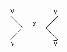
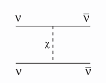
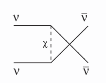
Figure 3: s-, t- and u-channel diagrams of $2\nu\leftrightarrow 2\bar{\nu}$ through majoron exchange.

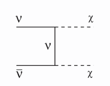
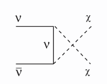
Figure 4: t- and u-channel diagrams of $\nu+\bar{\nu}\leftrightarrow 2\chi$ through neutrino exchange.

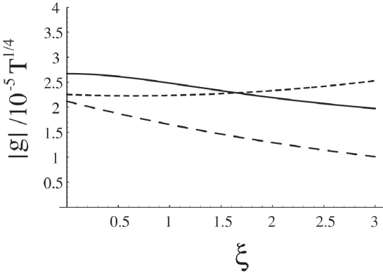
Figure 5: Upper bounds on $|g|$ obtained from the requirement that $L$-violating reactions, $2\nu\leftrightarrow 2\bar{\nu}$ and $\nu+\bar{\nu}\leftrightarrow 2\chi$, are out of equilibrium. Numerical and analytical bounds for the former reaction are shown as solid and long-dashed lines, respectively. The short-dashed line represents the constraint obtained numerically for the latter reaction.

5 Neutrino oscillations in primeval plasma

As is established now, neutrino mass eigenstates are related to the flavor eigenstates through the orthogonal matrix (we neglect a possible CP violation):

$$\nu_{a}=U_{aj}\,\nu_{j}$$ (37)

where $a=e,\mu,\tau$ and $j=1,2,3$. We have chosen the parameters so that in the limit of small mixing $\nu_{e}\approx\nu_{1}$, $\nu_{\mu}\approx\nu_{2}$, $\nu_{\tau}\approx\nu_{3}$. However, the mixing between neutrinos are known to be large and they cannot be taken as a dominant single mass eigenstate.

Kinetic equations for the density matrix of oscillating neutrinos can be written as [25, 23]:

$$i\dot{\rho}=[{\cal H}^{(1)},\rho]-i\{{\cal H}^{(2)},\rho\}$$ (38)

where the first commutator term includes the vacuum Hamiltonian and the effective potential of neutrinos in medium calculated in the first order in Fermi coupling constant, $G_{F}$ (weak interaction part) and in the second order in the coupling to majoron. The latter is given by Eq. (26) and does not contain off-diagonal terms if only one flavor coupling constant dominates. The weak interaction potential contains off-diagonal terms of the same order of magnitude as diagonal ones because of universal coupling of $W$ and $Z$ bosons to all neutrino flavors. Their explicit expressions can be found e.g. in Ref. [7]. In what follows we will skip upper indices $(1)$ and $(2)$ at ${\cal H}$.

The second anti-commutator term in Eq. (38) describes breaking of coherence induced by neutrino scattering and annihilation as well as neutrino production by collisions in primeval plasma. It includes imaginary part of the Hamiltonian calculated in the second order in $G_{F}$ and the fourth order terms in neutrino-majoron coupling $g$ related to neutrino-neutrino scattering through majoron exchange. If majorons were abundant in the primeval plasma the processes of neutrino-majoron scattering should also be included.

Since the “atmospheric” neutrino mass difference is much larger than the “solar” one, we may simplify the problem considering the process in two steps. First, oscillations between $\nu_{\tau}$ and $\nu_{\mu}$ were switched-on. This started at temperatures about 10-15 MeV and might lead to equilibration of tauonic and muonic charge asymmetries if these asymmetries were not erased by reactions (27). Later at $T\leq 3$ MeV, oscillations would start between $\nu_{e}$ and $\nu_{\mu^{\prime}}$, which is a certain mixture of $c\nu_{\tau}+s\nu_{\mu}$. This process is potentially dangerous for BBN because it could change number density and spectrum of $\nu_{e}$ and $\bar{\nu}_{e}$.

If mixing is effective only between two neutrinos, the density matrix is $2\times 2$ and kinetic equations for its components have the form:

$$iHx\partial_{x}\rho_{\mu\mu} = {\cal H}_{\mu\tau}\rho_{\tau\mu}-{\cal H}_{\tau\mu}\rho_{\mu\tau}-iI^{(coll)}_{\mu\mu}$$ (39)

$$iHx\partial_{x}\rho_{\tau\tau} = {\cal H}_{\tau\mu}\rho_{\mu\tau}-{\cal H}_{\mu\tau}\rho_{\tau\mu}-iI^{(coll)}_{\tau\tau}$$ (40)

$$iHx\partial_{x}\rho_{\mu\tau} = \left({\cal H}_{\mu\mu}-{\cal H}_{\tau\tau}\right)\rho_{\mu\tau}+{\cal H}_{\mu\tau}\left(\rho_{\tau\tau}-\rho_{\mu\mu}\right)-i\Gamma_{\mu\tau}\rho_{\mu\tau}$$ (41)

where $H$ and $x$ are defined below Eq. (28), ${\cal H}_{ab}=V_{ab}+\sum_{j=2,3}U_{aj}U_{bj}m^{2}_{j}/2E$, $U_{aj}$ are matrix elements of the mixing matrix; in the case under consideration $U_{\mu 2}=U_{\tau 3}=\cos\theta\equiv c$ and $U_{\mu 3}=-U_{\tau 2}=\sin\theta\equiv s$. The coherence breaking terms are given by the usual collision integrals $I^{(coll)}$ in the equations for the diagonal components and by

$$\Gamma_{\mu\tau}=1.1\cdot 10^{-22}(y/x^{5})\,{\rm MeV}$$ (42)

for the non-diagonal component $\rho_{\mu\tau}=\rho_{\tau\mu}^{*}$. In the expression for $\Gamma_{\mu\tau}$ we neglected the contribution from the majoron related processes. The effective potential $V_{ab}$ contains contributions from the usual weak interactions and from the neutrino-majoron interactions (26). We assume that the weak part is dominated by the charge asymmetric contribution, which is true in the case of a large charge asymmetry:

$$V^{(w)}_{ab}=1.5\,C_{1}\,G_{F}T^{3}\int d{\bf y}\left(\rho_{ab}-\bar{\rho}_{ab}\right)\equiv B\int d{\bf y}\left(\rho_{ab}-\bar{\rho}_{ab}\right).$$ (43)

with $C_{1}$ defined in Eq. (6), $d{\bf y}=d^{3}{\bf y}/(2\pi)^{3}$, $\bar{\rho}$ is the antineutrino density matrix, and the coefficient 1.5 comes from $(11/4)\cdot 2\,\zeta(3)/\pi^{2}$, i.e. from normalization to photon number density.

Equations (39-41) can be solved numerically but we can make reasonable estimates analytically in the following way (for more details see e.g. Refs. [1, 26]). In the case of strong coherence breaking, i.e. $\Gamma_{\mu\tau}\gg H$, Eq. (41) can be formally solved in the stationary point approximation i.e. putting r.h.s. equal zero. In this way we obtain:

$$\rho_{\mu\tau}=\frac{{\cal H}_{\mu\tau}\left(\rho_{\mu\mu}-\rho_{\tau\tau}\right)}{{\cal H}_{\mu\mu}-{\cal H}_{\tau\tau}-i\Gamma_{\mu\tau}}\approx\frac{\rho_{\mu\mu}-\rho_{\tau\tau}}{V_{\mu\mu}-V_{\tau\tau}}\,\left(V_{\mu\tau}+\frac{\delta m_{32}^{2}}{4E}\,s_{2}\right)\,\left(1+\frac{i\Gamma_{\mu\tau}-c_{2}\delta m_{32}^{2}/2E}{V_{\mu\mu}-V_{\tau\tau}}\right)$$ (44)

where $\delta m_{32}^{2}\equiv m_{3}^{2}-m_{2}^{2}$, $s_{2}=\sin 2\theta$ and $c_{2}=\cos 2\theta$.

This expression could be substituted into Eqs. (39) and (40) for the diagonal components but one cannot obtain the closed equations for the latter because the potential $V_{\mu\tau}$ contains an integral from $\rho_{\mu\tau}$ over momentum, see Eq. (43). We assume for simplicity that only weak-interaction potential has noticeable off-diagonal components, i.e. $V_{\mu\tau}\simeq V_{\mu\tau}^{(w)}$. It can be true if e.g. $|g_{\tau\tau}|\gg|g_{\mu\mu}|$. To express $V_{\mu\tau}$ through diagonal components we integrate Eq. (44) and similar equation for $\bar{\rho}_{\mu\tau}$ over momentum and subtract one from the other. To simplify the expressions let us present the diagonal part of the potential as a sum of charge symmetric (majoron) and antisymmetric (weak) parts:

$$V_{\mu\mu}-V_{\tau\tau}\equiv V_{+}^{(\chi)}+V_{-}^{(w)}$$ (45)

where the charge asymmetric part $V_{-}^{(w)}$ can be separated into two terms containing integrals from neutrino and antineutrino elements of the density matrix (see Eq. (43)), $V_{-}^{(w)}=V_{\nu}-\bar{V}_{\nu}$.

After straightforward calculations we obtain:

$$V_{\mu\tau}=\frac{V_{+}^{(\chi)\,2}-(V_{\nu}-\bar{V}_{\nu})^{2}}{V_{+}^{(\chi)}(V_{+}^{(\chi)}-V_{\nu}-\bar{V}_{\nu})}\int d{\bf y}\,\frac{s_{2}\delta m_{32}^{2}B}{4E}\left[\frac{\rho_{\mu\mu}-\rho_{\tau\tau}}{V_{+}^{(\chi)}+V_{\nu}-\bar{V}_{\nu}}\left(1+\frac{i\Gamma_{\mu\tau}-\delta m_{32}^{2}c_{2}/2E}{V_{+}^{(\chi)}+V_{\nu}-\bar{V}_{\nu}}\right)\right.$$

$$\left.-\frac{\bar{\rho}_{\mu\mu}-\bar{\rho}_{\tau\tau}}{V_{+}^{(\chi)}-V_{\nu}+\bar{V}_{\nu}}\left(1+\frac{i\bar{\Gamma}_{\mu\tau}-\delta m_{32}^{2}c_{2}/2E}{V_{+}^{(\chi)}-V_{\nu}+\bar{V}_{\nu}}\right)\right].$$ (46)

This result is valid if $|V_{+}^{(\chi)}|\geq|V_{-}^{(w)}|$. In the case of the usual weak interactions considered e.g. in Refs. [7, 8] the situation is opposite, $|V_{+}^{(\chi)}|\ll|V_{-}^{(w)}|$, and the character of the approximate analytical solution is completely different.

For a rough estimate let us assume that $|V_{+}^{(\chi)}|>|V_{-}^{(w)}|$ and $|V_{+}^{(\chi)}|>|\delta m_{32}^{2}|/2E$, while $|V_{\mu\tau}|<|s_{2}\delta m_{32}^{2}|/2E$, as follows from Eq. (46). In this case we find

$$Hx\partial_{x}\rho_{\mu\mu}=-\left(\frac{\delta m_{32}^{2}}{4E}\,s_{2}\right)^{2}\,\frac{\Gamma_{\mu\tau}(\rho_{\mu\mu}-\rho_{\tau\tau})}{(V_{\mu\mu}^{(\chi)}-V_{\tau\tau}^{(\chi)})^{2}}-I^{(coll)}_{\mu\mu}.$$ (47)

The evolution of the difference of muonic and tauonic charges is determined by

$$L^{(\mu\tau)} \equiv \int d{\bf y}\,L_{\bf y}^{(\mu\tau)}\equiv\int d{\bf y}\left(\rho_{\mu\mu}-\rho_{\tau\tau}-\bar{\rho}_{\mu\mu}+\bar{\rho}_{\tau\tau}\right).$$ (48)

The collision integrals disappear from the time derivative of this difference since weak interactions conserve leptonic charges and majoron induced processes are assumed to be suppressed, see sec. 4 and in particular Eq. (32). The evolution of $L$ is governed by the equation:

$$\frac{dL^{(\mu\tau)}}{dx}\approx\left(\frac{|g|}{1.5\times 10^{-7}}\right)^{-4}\left(\frac{\delta m_{32}^{2}}{2.5\times 10^{-3}{\rm eV}^{2}}\right)^{2}\int\frac{d{\bf y}}{y}\,L_{\bf y}^{(\mu\tau)}$$ (49)

and for the majoron coupling constant bounded by the conditions presented above, $L^{(\mu\tau)}$ remains practically constant till nucleosynthesis epoch, i.e. $x\sim 1$.

We have performed numerical calculations to solve Eqs. (39-41) in a similar way to Ref. [7]. The coupling constant matrix $g_{ab}$ is assumed to take the form: $g_{ab}=g\,\delta_{a\tau}\delta_{b\tau}$, for simplicity. The evolution of dimensionless chemical potentials $\xi_{\mu}$ and $\xi_{\tau}$ for several values of $|g|$ are shown in Fig. 6. One can see that the lepton asymmetries of $\nu_{\mu}$ and $\nu_{\tau}$ equilibrate around $T\sim 12$MeV when $|g|=0$. We have checked that the evolution remains the same for $|g|<10^{-8}$. As $|g|$ increases, the oscillations become less efficient and completely stop for $|g|\mathop{}_{\textstyle\sim}^{\textstyle>}10^{-7}$, which well agrees with the analytical estimates. It should be also noted that the lower bound on $|g|$ obtained from Eq. (49) does not depend on the magnitude of the initial lepton asymmetries. We have checked that the oscillations are similarly stuck for $|g|\mathop{}_{\textstyle\sim}^{\textstyle>}10^{-7}$ even if the initial lepton asymmetries are taken to be smaller. The only difference is the temperature at which the asymmetries equilibrate when $g=0$.

We can repeat the same arguments for oscillations between $\nu_{e}$ and $\nu_{\mu^{\prime}}$. The squared mass difference and mixing angle parameters for the oscillations between $\nu_{e}$ and $\nu_{\mu^{\prime}}$ are $\delta m_{21}^{2}\equiv m_{2}^{2}-m_{1}^{2}=7.3\times 10^{-5}{\rm eV}^{2}$ and $\sin^{2}\theta=0.315$ [27]. The coupling constant matrix $g_{ab}$ is similarly approximated to be $g_{ab}=g\,\delta_{a\mu^{\prime}}\delta_{b\mu^{\prime}}$. Also the effective potential induced by the energy densities of electrons and positrons is taken into account, since here we consider oscillations including $\nu_{e}$. The lower bound of $|g|$ becomes slightly relaxed due to the smaller mass difference, as can be seen from Fig. 7. The reason why the lepton asymmetries of $\nu_{e}$ and $\nu_{\mu^{\prime}}$ are not equilibrated completely when $g=0$ is that the mixing angle we adopt is not maximal.

Lastly, we comment on the form of the coupling matrix, $g_{ab}$, for which the $(\nu_{e}-\nu_{\mu^{\prime}})$-transformations are suppressed and, consequently, a large lepton asymmetry of the universe is allowed. So far we have assumed that $g_{ab}$ is diagonal in order to deal with both $\nu_{\tau}-\nu_{\mu}$ and $\nu_{e}-\nu_{\mu^{\prime}}$ oscillations similarly. However, in fact, a coupling matrix with more generic form works as well. We would like to stress that the equilibration of the muonic and tauonic lepton asymmetries is not harmful to our purpose, as long as these asymmetries are not erased through either oscillations or by the reactions shown in Figs. 3 and 4. Therefore we do not have to assume the hierarchical structure in $g_{\tau\tau}$, $g_{\mu\tau}$, and $g_{\mu\mu}$, and they are constrained only by the astrophysical bounds:

$$|g_{ab}|<5\times 10^{-6}$$ (50)

with $(a,b)=\{(\tau,\tau),(\mu,\tau),(\mu,\mu)\}$. In order to suppress the oscillations between $\nu_{e}$ and $\nu_{\mu^{\prime}}$, at least one of these coupling constants should be larger than $\sim 10^{-7}$, while $|g_{ee}|$, $|g_{e\mu}|$, and $|g_{e\tau}|$ must be much smaller than $\sim 10^{-7}$. Thus we conclude that the coupling matrix suitable for our purpose should satisfy:

$$|g_{ee}|,~{}|g_{e\mu}|,~{}|g_{e\tau}| \ll 10^{-7},$$

$$10^{-7}\mathop{}_{\textstyle\sim}^{\textstyle<} {\rm Max}\,\left[\,|g_{\tau\tau}|,~{}|g_{\mu\tau}|,~{}|g_{\mu\mu}|\,\right] \mathop{}_{\textstyle\sim}^{\textstyle<}5\times 10^{-6}.$$ (51)

In the simplest class of majoron models, the coupling matrix, $g_{ab}$, is proportional to the neutrino mass matrix $(m_{\nu})_{ab}$. In particular, for the normal mass hierarchy, $m_{1}<m_{2}<m_{3}$, the reconstructed mass matrix is often parametrized as [28]

λ11λ11)proportional-to𝑔subscript𝑚𝜈proportional-to00𝜆011𝜆11orfragments 𝜆11𝜆11\displaystyle g\propto m_{\nu}\propto\left(\begin{tabular}[]{lll}0&0&$\lambda$\\ 0&1&1\\ $\lambda$&1&1\end{tabular}\right)~{}{\rm or}~{}\left(\begin{tabular}[]{lll}$\lambda^{2}$&$\lambda$&$\lambda$\\ $\lambda$&1&1\\ $\lambda$&1&1\\ \end{tabular}\right)

λ2λλλ2λλ (58)

with $\lambda\sim 0.2$. Therefore the coupling matrix of this type can satisfy the conditions (51). Of course, in the more involved models, the coupling matrix is not necessarily proportional to the neutrino mass matrix.

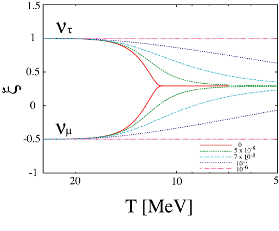
Figure 6: The evolutions of $\xi_{\mu}$ and $\xi_{\tau}$ for several values of $|g|$ for the maximal mixing and $\delta m_{32}^{2}=2.5\times 10^{-3}{\rm eV}^{2}$. The initial conditions are $\xi_{\mu}=-0.5$ and $\xi_{\tau}=1.0$.

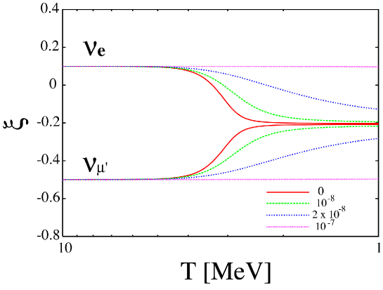
Figure 7: The evolutions of $\xi_{e}$ and $\xi_{\mu^{\prime}}$ for several values of $|g|$ with $\sin^{2}\theta=0.315$ and $\delta m_{21}^{2}=7.3\times 10^{-5}{\rm eV}^{2}$. The initial conditions are $\xi_{e}=0.1$ and $\xi_{\mu^{\prime}}=-0.5$.

6 Discussions and Conclusions

In the preceding sections we have shown that neutrino oscillations in primordial plasma can be blocked by an introduction of the neutrino-majoron interaction with a moderate value of coupling constants, $|g|\mathop{}_{\textstyle\sim}^{\textstyle<}5\cdot 10^{-6}$. Here let us take up the case of $|g|\mathop{}_{\textstyle\sim}^{\textstyle>}10^{-5}$. For a definite discussion, we assume that the elements of coupling constant matrix whose indices involve electronic neutrino are much smaller than the other elements, i.e. $|g_{ee}|,~{}|g_{ea}|\ll|g_{ab}|$ with $(a,b)=\{(\tau,\tau),(\mu,\tau),(\mu,\mu)\}$, so the electron type lepton number conserves during the relevant BBN epoch. As we have seen in section 4, the muonic and/or tauonic lepton number is not conserved for $|g_{ab}|\mathop{}_{\textstyle\sim}^{\textstyle>}10^{-5}$. The fate of the large degeneracy in $\nu_{\mu}$ and $\nu_{\tau}$ depends on whether this $L$-violating interaction reached equilibrium before or after $\nu_{\mu}$ and $\nu_{\tau}$ decoupled from the thermal bath.

First let us consider the former scenario. Since $\nu_{\mu}$ and $\nu_{\tau}$ kept on to be in strong contact with the primeval plasma when the $L$-violating interactions were efficient, the muonic and/or tauonic lepton asymmetry vanished and thereby heated the plasma. At the same time majorons were abundantly produced and contributed to the effective number of neutrino species as $\Delta N_{\nu}=4/7$. The CP asymmetric part of the effective potential of neutrino due to the muonic and tauonic lepton asymmetries vanished, but there would be a similar (but possibly smaller) term due to the charge asymmetry of $\nu_{e}$ (see Eqs. (7) and (8)). Also there exists the contribution the the effective potential due to abundant majorons in the plasma (see Eq. (25)). A further important point is that $L$-violating processes, shown in Fig. 3, induces the effective potential between neutrino and antineutrino, since $\langle a^{\dagger}b\rangle$ no longer vanishes. However, neutrino oscillations between $\nu_{e}$ and $\nu_{\mu^{\prime}}$ can be treated in the same way as before, since electron type lepton number remains a well conserved quantity. Therefore, we can deduce from the previous results that neutrino oscillations between $\nu_{e}$ and $\nu_{\mu^{\prime}}$ are blocked and $\xi_{e}$ remains intact. It should be noted that equilibrium majorons, instead of excessive $\nu_{\mu}$ and $\nu_{\tau}$, contribute to the extra radiation, which speeds up the expansion rate, and that its contribution, $\Delta N_{\nu}=4/7$, well satisfies the constraint shown in Eq. (3).

Next we discuss the other possibility that the $L$-violating interactions come to thermal equilibrium after decoupling of $\nu_{\mu}$ and $\nu_{\tau}$. Majorons are also produced, as in the previous case. However, since $\nu_{\mu}$ and $\nu_{\tau}$ cannot exchange energy with the primeval plasma, the total energy of majorons, $\nu_{\mu}$ and $\nu_{\tau}$ must be conserved. Therefore the excessive energy previously stored in $\nu_{\mu}$ and $\nu_{\tau}$ is redistributed among majorons, $\nu_{\mu}$, and $\nu_{\tau}$, and their distribution would be like Eq. (33) but without any charge asymmetry, i.e. with $\xi=\bar{\xi}$. It is thus clear that $\Delta N_{\nu}$ remains unchanged before and after $L$-violating interaction comes into equilibrium. Our concern here is whether the modified distribution of $\nu_{\mu^{\prime}}$ affects that of $\nu_{e}$ through neutrino oscillations. However, the oscillations are blocked on the same ground.

In connection with the second case, there is an interesting possibility that the majoron-exchange reactions: $\nu_{\mu,\tau}\bar{\nu}_{\mu,\tau}\leftrightarrow\nu_{e}\bar{\nu}_{e}$, $\nu_{\mu,\tau}\nu_{\mu,\tau}\leftrightarrow\nu_{e}\nu_{e}$, $\nu_{\mu,\tau}\nu_{\mu,\tau}\leftrightarrow\bar{\nu}_{e}\bar{\nu}_{e}$, $\bar{\nu}_{\mu,\tau}\bar{\nu}_{\mu,\tau}\leftrightarrow\nu_{e}\nu_{e}$ and $\bar{\nu}_{\mu,\tau}\bar{\nu}_{\mu,\tau}\leftrightarrow\bar{\nu}_{e}\bar{\nu}_{e}$, could produce additional electronic neutrinos and antineutrinos. These processes can proceed if $|g_{ee}|$ and $|g_{ea}|$ with $a=\mu,~{}\tau$ are sizable $\mathop{}_{\textstyle\sim}^{\textstyle>}10^{-5}$. If this is the case, the relative abundance of $\nu_{e}$ and $\bar{\nu}_{e}$ with respect to photons and electrons would be larger than in the standard model. This would lead to a later neutron-proton freezing and to a smaller number density of survived neutrons, which might compensate the effect of additional energy density stored in all species of neutrinos and majorons and even overshoot it. Then we do not need to suppress neutrino oscillations, therefore the coupling constant matrix $g_{ab}$ is allowed to take rather arbitrary values as long as the $L$-violating processes come into equilibrium after decoupling of muonic and tauonic neutrinos.

Thus our examination indicates that a conspiracy between the speed-up effect and the shift of $\beta$ equilibrium is possible for $|g_{ab}|\mathop{}_{\textstyle\sim}^{\textstyle>}10^{-5}$, as long as $|g_{ee}|,~{}|g_{ea}|\ll|g_{ab}|$ with $a,~{}b=\mu,~{}\tau$. Furthermore, even for $|g_{ee}|,~{}|g_{ea}|\mathop{}_{\textstyle\sim}^{\textstyle>}10^{-5}$, such a cancellation might be possible in a somewhat different way. This considerably extends the allowed parameter space, although rigorous study might be necessary to obtain further quantitative results.

In this paper we have shown that the hypothetical neutrino-majoron interaction can suppress neutrino oscillations in the primordial plasma to prevent lepton asymmetries of all neutrino species from being equilibrated. The exact form of the effective potential induced by this interaction is calculated. We have found an allowed range of the coupling constant: $10^{-7}<|g|<5\cdot 10^{-6}$ (more precisely, see Eq. (51)), which satisfies the astrophysical bounds and makes the scenario operative. For the coupling constant in this range, $\nu_{e}-\nu_{\mu^{\prime}}$ oscillation in the early Universe is blocked, thereby keeping the cosmological lepton asymmetry of electron type unchanged. The upper bound comes from the requirement that lepton number is effectively conserved, and the lower bound is obtained from the study of the evolution of the lepton asymmetries both analytically and numerically, in two flavor approximation. The constant matrix in the simplest class of majoron models can satisfy the desired constraints, in the case of the normal mass hierarchy. Furthermore, even for $|g|\mathop{}_{\textstyle\sim}^{\textstyle>}10^{-5}$, the large energy density necessary to cancel the effect of $\xi_{e}$ can be supplied by majorons, $\nu_{\mu}$ and $\nu_{\tau}$, even if muonic and/or tauonic lepton asymmetries were erased. Thus we conclude that an addition of the majoron field to the standard model can reopen a possibility that the effect of $\xi_{e}$ is compensated by large $\xi_{\mu,\tau}$ (or by the extra energy of majoron itself), thereby curing a probable discrepancy between the BBN and CMBR.

Appendix A Derivation of effective potential due to majoron-neutrino interaction

Here we present the derivation of the effective potentials Eqs. (23) and (25). First the notations and conventions that we adopt here, are listed. The metric is taken to be $(-,+,+,+)$. The gamma matrices in the chiral representation are

$$\gamma^{0}=-i\left(\begin{array}[]{cc}0&1\\ 1&0\end{array}\right),~{}~{}~{}\gamma^{i}=-i\left(\begin{array}[]{cc}0&\sigma_{i}\\ -\sigma_{i}&0\end{array}\right),~{}~{}~{}\gamma_{5}=\left(\begin{array}[]{cc}1&0\\ 0&-1\end{array}\right),$$ (65)

where $\sigma_{i}$ are the Pauli matrices. The gamma matrices in the Dirac representation are related to those in the chiral representation as

$$\gamma^{\mu}_{\rm Dirac}=U\gamma^{\mu}_{\rm chiral}U^{\dagger},~{}~{}~{}U=\frac{1}{\sqrt{2}}\left(\begin{array}[]{cc}1&1\\ 1&-1\end{array}\right),$$ (68)

and they are given by

$$\gamma^{0}=-i\left(\begin{array}[]{cc}1&0\\ 0&-1\end{array}\right),~{}~{}~{}\gamma^{i}=i\left(\begin{array}[]{cc}0&\sigma_{i}\\ -\sigma_{i}&0\end{array}\right),~{}~{}~{}\gamma_{5}=\left(\begin{array}[]{cc}0&1\\ 1&0\end{array}\right).$$ (75)

The charge conjugation matrix $C$ is defined as

$$C\equiv i\gamma^{2}\gamma^{0}=\left\{\begin{array}[]{ll}-i\left(\begin{array}[]{cc}\sigma_{2}&0\\ 0&-\sigma_{2}\end{array}\right)&{\rm(chiral)}\\ &\\ -i\left(\begin{array}[]{cc}0&\sigma_{2}\\ \sigma_{2}&0\end{array}\right)&{\rm(Dirac)}\end{array}\right..$$ (83)

Hereafter we work with the gamma matrices in the Dirac representation. The momentum expansion of a free Dirac field $\psi(x)$ with mass $m$ is given by

$$\psi(x) = \sum_{s}\int d{\bf p}\left(a({\bf p},s)u({\bf p},s)e^{-iE_{\bf p}t+i{\bf p}\,{\bf x}}+b^{\dagger}({\bf p},s)v({\bf p},s)e^{iE_{\bf p}t-i{\bf p}\,{\bf x}}\right),$$ (84)

$$= \sum_{s}\int d{\bf p}\left(a({\bf p},s)u({\bf p},s)+b^{\dagger}(-{\bf p},s)v(-{\bf p},s)\right)e^{-ip^{0}t+i{\bf p}\,{\bf x}},$$

where we defined $p^{0}\equiv\epsilon_{p}E_{\bf p}=\epsilon_{p}\sqrt{{\bf p}^{2}+m^{2}}$ with $\epsilon_{p}=\pm 1$. The sign of $\epsilon_{p}$ is chosen so that the positive and negative-energy solutions are reproduced. $s=\pm$ describes the sign of the spin projection eigenvalue, and we have used the notation $d{\bf p}\equiv d^{3}{\bf p}/(2\pi)^{3}$. The Dirac spinors $u({\bf p},s)$ and $v({\bf p},s)$ take the form,

$$u({\bf p},s) = \frac{1}{\sqrt{2E_{\bf p}(E_{\bf p}+m)}}\left(\begin{array}[]{c}E_{\bf p}+m\\ -{\bf p}\cdot{\bf\sigma}\end{array}\right)\chi_{u}(s),$$ (87)

$$v({\bf p},s) = \frac{1}{\sqrt{2E_{\bf p}(E_{\bf p}+m)}}\left(\begin{array}[]{c}-{\bf p}\cdot{\bf\sigma}\\ E_{\bf p}+m\end{array}\right)\chi_{v}(s).$$ (90)

The two-component spinors $\chi_{u}(s)$ and $\chi_{v}(s)$ are not independent but related to each other through: $\chi_{v}(s)=-i\sigma_{2}\chi_{u}(s)^{*}$. If we choose them to be eigenstates of the helicity operator ${\bf p\cdot\sigma}/|{\bf p}|$, they are

$$\chi_{u}(+) = \left(\begin{array}[]{c}e^{-i\varphi/2}\cos{\frac{\theta}{2}}\\ e^{i\varphi/2}\sin{\frac{\theta}{2}}\end{array}\right),~{}~{}~{}\chi_{u}(-)=\left(\begin{array}[]{c}-e^{-i\varphi/2}\sin{\frac{\theta}{2}}\\ e^{i\varphi/2}\cos{\frac{\theta}{2}}\end{array}\right),$$ (95)

$$\chi_{v}(+) = \left(\begin{array}[]{c}-e^{-i\varphi/2}\sin{\frac{\theta}{2}}\\ e^{i\varphi/2}\cos{\frac{\theta}{2}}\end{array}\right),~{}~{}~{}\chi_{v}(-)=\left(\begin{array}[]{c}-e^{-i\varphi/2}\cos{\frac{\theta}{2}}\\ -e^{i\varphi/2}\sin{\frac{\theta}{2}}\end{array}\right),$$ (100)

where $\theta$ and $\varphi$ are defined as ${\bf p}=|{\bf p}|(\sin\theta\cos\varphi,\sin\theta\sin\varphi,\cos\theta)$. For flipped momentum $-{\bf p}$, $\{\theta,\varphi\}$ should be replaced with $\{\pi-\theta,\varphi+\pi\}$.

In deriving the effective potential, the neutrino field $\nu(x)$ is approximated to be a massless left-handed field :

$$\nu_{i}(x) = \int d{\bf p}\left(a_{i}({\bf p})u_{\bf p}+b_{i}({-{\bf p}})^{\dagger}v_{-{\bf p}}\right)e^{-ip^{0}t+i{\bf p}\,{\bf x}},$$ (101)

where

$$u_{\bf p} \equiv \frac{1+\gamma_{5}}{2}u({\bf p},-)=\frac{1}{\sqrt{2}}\left(\begin{array}[]{c}1\\ 1\end{array}\right)\chi_{u}(-),$$ (104)

$$u_{-{\bf p}} \equiv \frac{1+\gamma_{5}}{2}u(-{\bf p},-)=\frac{i}{\sqrt{2}}\left(\begin{array}[]{c}1\\ 1\end{array}\right)\chi_{u}(+),$$ (107)

$$v_{{\bf p}} \equiv \frac{1+\gamma_{5}}{2}v({\bf p},+)=\frac{1}{\sqrt{2}}\left(\begin{array}[]{c}1\\ 1\end{array}\right)\chi_{u}(-),$$ (110)

$$v_{-{\bf p}} \equiv \frac{1+\gamma_{5}}{2}v(-{\bf p},+)=\frac{i}{\sqrt{2}}\left(\begin{array}[]{c}1\\ 1\end{array}\right)\chi_{u}(+).$$ (113)

The annihilation and creation operators $a$, $b$, $a^{\dagger}$ and $b^{\dagger}$ satisfy the anticommutation relations.

$$\left\{a_{i}({\bf p}),\,a_{j}({\bf q})^{\dagger}\right\} = (2\pi)^{3}\delta_{ij}\,\delta^{(3)}({\bf p}-{\bf q}),$$

$$\left\{b_{i}({\bf p}),\,b_{j}({\bf q})^{\dagger}\right\} = (2\pi)^{3}\delta_{ij}\,\delta^{(3)}({\bf p}-{\bf q}),$$

$${\rm others} = 0.$$ (114)

Similarly, the momentum expansion of the free majoron field is

$$\chi(x) = \int d{\bf p}\left(a_{\chi}({\bf p})u_{\chi}({\bf p})+a_{\chi}({-{\bf p}})^{\dagger}v_{\chi}({-{\bf p}})\right)e^{-ip^{0}t+i{\bf p}\,{\bf x}},$$ (115)

where

$$u_{\chi}({\bf p})=v_{\chi}({\bf p})=\frac{1}{\sqrt{2E_{\bf p}}}.$$ (116)

The annihilation and creation operators $a_{\chi}$, $a_{\chi}^{\dagger}$ satisfy the commutation relations:

$$\left[a_{\chi}({\bf p}),\,a_{\chi}({\bf q})^{\dagger}\right] = (2\pi)^{3}\,\delta^{(3)}({\bf p}-{\bf q}),$$

$${\rm others} = 0.$$ (117)

Next we derive the effective Hamiltonian Eq. (20). The equation of motion for the majoron field $\chi$ is

$$\partial_{\mu}\partial^{\mu}\chi=-\frac{i}{2}\left(g_{ab}\,\nu_{a}^{T}C\nu_{b}+g_{ab}^{*}\,\nu_{b}^{\dagger}C\nu_{a}^{*}\right).$$ (118)

To solve this equation, we define the majoron and neutrino fields in momentum space :

$$\chi(x) = \int\frac{d^{4}p}{(2\pi)^{4}}\,\tilde{\chi}(p)\,e^{ipx},$$

$$\nu_{a}(x) = \int\frac{d^{4}p}{(2\pi)^{4}}\,\tilde{\nu}_{a}(p)\,e^{ipx}.$$ (119)

Then the solution of Eq. (118) is

$$\tilde{\chi}(p) = \frac{i}{2p^{2}}\int\frac{d^{4}q}{(2\pi)^{4}}\left\{g_{ab}\,\tilde{\nu}_{a}(p-q)^{T}C\tilde{\nu}_{b}(q)+g_{ab}^{*}\,\tilde{\nu}_{b}(-p+q)^{\dagger}C\tilde{\nu}_{a}^{*}(-q)\right\}.$$ (120)

Thus the effective Hamiltonian is:

$${\cal H}_{\rm eff}^{(\nu\nu)} = -\int d^{3}{\bf x}\,{\cal L}_{\rm eff}^{(\nu\nu)},$$ (121)

$$= -\frac{1}{2}\int d^{3}{\bf x}\,\frac{i}{2}\int\frac{d^{4}p}{(2\pi)^{4}}\,e^{ipx}\frac{i}{2p^{2}}\int\frac{d^{4}q}{(2\pi)^{4}}\left\{g_{ab}\,\tilde{\nu}_{a}(p-q)^{T}C\tilde{\nu}_{b}(q)\right.$$

$$\left.+g_{ab}^{*}\,\tilde{\nu}_{b}(-p+q)^{\dagger}C\tilde{\nu}_{a}^{*}(-q)\right\}\int\frac{d^{4}r}{(2\pi)^{4}}\,e^{irx}\int\frac{d^{4}s}{(2\pi)^{4}}\,e^{isx}$$

$$\times\left\{g_{cd}\,\tilde{\nu}_{c}(r)^{T}C\tilde{\nu}_{d}(s)+g_{cd}^{*}\,\tilde{\nu}_{d}(-s)^{\dagger}C\tilde{\nu}_{c}^{*}(-r)\right\}.$$

where we substituted Eq. (120) into the second equation. Note that the numerical factor $1/2$ is inserted in front of the last equation. In a first-order perturbative approximation the neutrino and majoron fields can be set to be free fields:

$$\tilde{\nu}_{i}(p) = 2\pi\delta(p^{0}-\epsilon_{p}E_{\bf p})\,\nu_{i}({\bf p}),$$

$$\tilde{\chi}(p) = 2\pi\delta(p^{0}-\epsilon_{p}E_{\bf p})\,\chi({\bf p}),$$ (122)

where

$$\nu_{i}({\bf p}) = a_{i}({\bf p})u_{\bf p}+b_{i}(-{\bf p})^{\dagger}v_{-{\bf p}},$$

$$\chi({\bf p}) = a_{\chi}({\bf p})u_{\chi}({\bf p})+a_{\chi}(-{\bf p})^{\dagger}v_{\chi}({-{\bf p}}).$$ (123)

Thus the effective Hamiltonian becomes

$${\cal H}_{\rm eff}^{(\nu\nu)}(t) = -\frac{1}{16}\int d{\bf p}\,d{\bf q}\,d{\bf r}\,d{\bf s}\,\,(2\pi)^{3}\delta^{(3)}({\bf p+q+r+s})\,e^{-iE_{\rm tot}t}$$ (124)

$$~{}~{}~{}~{}~{}~{}~{}~{}\times\frac{F({\bf p},{\bf q})F({\bf r},{\bf s})}{\epsilon_{p}\epsilon_{q}E_{\bf p}E_{\bf q}(1-\epsilon_{p}\epsilon_{q}\cos\theta_{\bf pq})},$$

where

$$E_{\rm tot} = \epsilon_{p}E_{\bf p}+\epsilon_{q}E_{\bf q}+\epsilon_{r}E_{\bf r}+\epsilon_{s}E_{\bf s},$$

$$\cos\theta_{\bf pq} \equiv \frac{{\bf p}\cdot{\bf q}}{\left|{\bf p}\right|\left|{\bf q}\right|},$$

$$F({\bf p},{\bf q}) \equiv g_{ab}\,\nu_{a}({\bf p})^{T}C\nu_{b}({\bf q})+g_{ab}^{*}\,\nu_{b}({\bf-q})^{\dagger}C\nu_{a}^{*}({\bf-p}).$$ (125)

Once the effective Hamiltonian is obtained, we can calculate the effective potential for neutrinos according to Ref. [23]. All we have to do is to evaluate

$$\left\langle\left[{\cal H}_{\rm eff}(t=0),a_{j}({\bf p})^{\dagger}a_{i}({\bf p})\right]\right\rangle = -(2\pi)^{3}\delta^{(3)}(0)\left[V_{\bf p},\rho_{\bf p}\right]_{ij},$$ (126)

where $\left[V_{\bf p}\right]_{ab}$ is the effective potential matrix. Using the anticommutation relations (A), we obtain the final result:

$$\left[V_{\bf p}^{(\nu\nu)}\right]_{ab}=\int d{\bf q}~{}~{}\frac{1}{4\left|{\bf p}\right|\left|{\bf q}\right|}\left[g^{\dagger}\left(\rho^{T}_{\bf q}+\overline{\rho}^{T}_{\bf q}\right)g\right]_{ab}.$$ (127)

Next we derive the effective Hamiltonian, which describes neutrino-majoron scattering. In this case we integrate out the neutrino field instead of majoron field. The equation of motion for the neutrino is

$$-i\gamma^{0}\gamma^{\mu}\partial_{\mu}\nu_{a}+i\chi g_{ab}^{*}C\nu_{b}^{*}=0.$$ (128)

The solution is then

$$\tilde{\nu}_{a}(p)=\frac{ip_{\mu}}{p^{2}}g_{ab}^{*}\int\frac{d^{4}q}{(2\pi)^{4}}\tilde{\chi}(p+q)\gamma^{\mu}\gamma^{0}C\tilde{\nu}_{b}^{*}(q).$$ (129)

Substituting this result into Eq. (19), we obtain the effective Hamiltonian:

$${\cal H}_{\rm eff}^{(\nu\chi)}(t) = -\frac{i}{2}\,g_{ab}g_{bc}^{*}\int d^{3}{\bf x}\int\frac{d^{4}p}{(2\pi)^{4}}\frac{d^{4}q}{(2\pi)^{4}}\frac{d^{4}r}{(2\pi)^{4}}\frac{d^{4}s}{(2\pi)^{4}}\,e^{i(p+q+r+s)x}$$ (130)

$$\times\,\tilde{\chi}(p)\tilde{\chi}(q)\,\overline{\tilde{\nu}}_{c}(-r)\gamma^{\mu}\tilde{\nu}_{a}(s)\,\frac{(q+r)_{\mu}}{(q+r)^{2}},$$

$$= -\frac{i}{2}\,\left[g^{\dagger}g\right]_{ab}\int d{\bf p}\,d{\bf q}\,d{\bf r}\,d{\bf s}\,\,(2\pi)^{3}\delta^{(3)}({\bf p+q+r+s})\,e^{-iE_{\rm tot}t}$$

$$\times\chi({\bf p})\chi({\bf q})\overline{\nu}_{a}(-{\bf r})\gamma^{\mu}\nu_{b}({\bf s})\,\left.\frac{(q+r)_{\mu}}{2q\cdot r}\right|_{q^{0}=\epsilon_{q}E_{\bf q},r^{0}=\epsilon_{r}E_{\bf r}},$$

where we take both neutrino and majoron fields to be on-shell in the second equation. Applying Eq. (126), we obtain the effective potential due to the neutrino-majoron scattering:

$$\left[V_{\bf p}^{(\nu\chi)}\right]_{ab}=\int d{\bf q}~{}~{}\frac{f_{\chi}({\bf q})}{4\left|{\bf p}\right|\left|{\bf q}\right|}\left[g^{\dagger}g\right]_{ab},$$ (131)

where the number density of majorons with momentum ${\bf p}$, $n_{\bf p}^{(\chi)}$, is defined as

$$\left\langle a^{\dagger}_{\chi}({\bf p})\,a_{\chi}({\bf p}^{\prime})\right\rangle = (2\pi)^{3}\delta^{(3)}({\bf p}-{\bf p}^{\prime})\,f_{\chi}({\bf p}).$$ (132)

Appendix B Invariant amplitude squared for $2\nu\leftrightarrow 2\bar{\nu}$

Here we calculate the invariant amplitude squared for the reaction, $2\nu\leftrightarrow 2\bar{\nu}$. Provided that the diagonal coupling constants are larger than the non-diagonal ones, and that one of the diagonal coupling constants dominates, we consider neutrinos of the flavor with the largest coupling. Hereafter we drop the sub-indices for flavor. The diagrams, which contribute to the reaction, are shown in Fig. 3.

The S-matrix and the invariant amplitude squared are related as

$$S_{\beta\alpha} = 2\pi(-i)\delta^{(4)}(p_{\beta}-p_{\alpha}){\cal M}_{\beta\alpha},$$

$$\left|M_{\rm inv}\right|^{2} = (2\pi)^{-6}\prod_{\alpha}\left[(2\pi)^{3}2E_{\alpha}\right]\prod_{\beta}\left[(2\pi)^{3}2E_{\beta}\right]\left|{\cal M}_{\beta\alpha}\right|^{2},$$ (133)

where $\alpha$ and $\beta$ represent symbolically the initial and final states . Each matrix element for s-, t- and u-channel diagrams is given as

$${\cal M}^{(s)}_{p_{3}p_{4},p_{1}p_{2}} = \frac{g^{2}}{(2\pi)^{3}}\frac{1}{(p_{1}+p_{2})^{2}}(u_{{\bf p}_{2}}^{T}Cu_{{\bf p}_{1}})(v_{{\bf p}_{4}}^{T}Cv_{{\bf p}_{3}}),$$

$${\cal M}^{(t)}_{p_{3}p_{4},p_{1}p_{2}} = -\frac{g^{2}}{(2\pi)^{3}}\frac{1}{(p_{1}-p_{3})^{2}}(v_{{\bf p}_{3}}^{T}Cu_{{\bf p}_{1}})(v_{{\bf p}_{4}}^{T}Cu_{{\bf p}_{2}}),$$

$${\cal M}^{(u)}_{p_{3}p_{4},p_{1}p_{2}} = \frac{g^{2}}{(2\pi)^{3}}\frac{1}{(p_{1}-p_{4})^{2}}(v_{{\bf p}_{4}}^{T}Cu_{{\bf p}_{1}})(v_{{\bf p}_{3}}^{T}Cu_{{\bf p}_{2}}),$$ (134)

where the four momenta satisfy the conservation condition, $p_{1}+p_{2}=p_{3}+p_{4}$. If we use the explicit expressions for $u_{\bf p}$ and $v_{\bf p}$ derived in the previous section, we obtain

$${\cal M}^{(s)}_{p_{3}p_{4},p_{1}p_{2}}+{\cal M}^{(t)}_{p_{3}p_{4},p_{1}p_{2}}+{\cal M}^{(u)}_{p_{3}p_{4},p_{1}p_{2}}=\frac{g^{2}}{(2\pi)^{3}}\frac{1}{\sqrt{E_{1}E_{2}E_{3}E_{4}}}\,\frac{3}{4}.$$ (135)

Substituting this result into Eq. (133), the invariant amplitude squared becomes

$$\left|M_{\rm inv}\right|^{2} = 9|g|^{4}.$$ (136)

Appendix C Formulas for the collisional integral in the Boltzmann approximation

Here we write down the formulas for the collisional integral in the Boltzmann approximation for completeness. For the derivation, see Ref. [29].

$$\int\frac{d^{3}{\bf y}_{2}}{y_{2}}\int\frac{d^{3}{\bf y}_{3}}{y_{3}}\int\frac{d^{3}{\bf y}_{4}}{y_{4}}e^{-y_{3}-y_{4}}\delta^{(4)}(y_{1}+y_{2}-y_{3}-y_{4}) = 4\pi^{2}e^{-y_{1}},$$

$$\int\frac{d^{3}{\bf y}_{1}}{y_{1}}\int\frac{d^{3}{\bf y}_{2}}{y_{2}}\int\frac{d^{3}{\bf y}_{3}}{y_{3}}\int\frac{d^{3}{\bf y}_{4}}{y_{4}}e^{-y_{3}-y_{4}}\delta^{(4)}(y_{1}+y_{2}-y_{3}-y_{4}) = 32\pi^{3}.$$ (137)

Acknowledgment

A.D. is grateful to the Research Center for the Early Universe of the University of Tokyo for the hospitality during the time when this work started. F. T. is grateful to M. Kawasaki and K. Ichikawa for useful discussions. F. T. would like to thank the Japan Society for the Promotion of Science for financial support.

References

- [1] A. D. Dolgov, Phys. Rept. 370 (2002) 333.
- [2] K. Kohri, M. Kawasaki and K. Sato, Astrophys. J. 490 (1997) 72.
- [3] V. Barger, J. P. Kneller, H. S. Lee, D. Marfatia and G. Steigman, Phys. Lett. B 566 (2003) 8.
- [4] S.H. Hansen, G. Mangano, A. Melchiorri, G. Miele and O. Pisanti, Phys. Rev. D 65 (2002) 023511.
-
[5]
J. A. Harvey and E. W. Kolb, Phys. Rev. D 24 (1981) 2090;
A.D. Dolgov, D.K. Kirilova, J. Moscow Phys. Soc. 1, (1991), 217;
A.D. Dolgov, Phys. Repts, 222 (1992) No. 6;
A. Casas, W. Y. Cheng and G. Gelmini, Nucl. Phys. B 538 (1999) 297;
J. March-Russell, H. Murayama and A. Riotto, JHEP 9911 (1999) 015;
J. McDonald, Phys. Rev. Lett. 84 (2000) 4798;
M. Kawasaki, F. Takahashi and M. Yamaguchi, Phys. Rev. D 66 (2002) 043516;
M. Yamaguchi, Phys. Rev. D 68 (2003) 063507;
T. Chiba, F. Takahashi and M. Yamaguchi, Phys. Rev. Lett. 92 (2004) 011301;
F. Takahashi and M. Yamaguchi, arXiv:hep-ph/0308173, Phys. Rev. D (to be published). -
[6]
SNO Collaboration, Phys. Rev. Lett. 89 (2002) 011301;
Phys. Rev. Lett. 89 (2002) 011302;
KamLAND Collaboration, Phys. Rev. Lett. 90 (2003) 021802;
S. Fukuda et al., Super-Kamiokande Coll., Phys. Lett. B539 (2002) 179;
B.T. Cleveland et al., Astrophys. J. 496, 505 (1998);
D.N. Abdurashitov et al., SAGE Coll., Phys. Rev. C60, 055801 (1999); astro-ph/0204245;
W. Hampel et al., GALLEX Coll., Phys. Lett. B447, 127 (1999);
C. Cattadori, GNO Coll., Nucl. Phys. B (Proc. Suppl.) 110 (2002) 311.
Super-Kamiokande Coll., Y. Fukuda et al., Phys. Rev. Lett. 81 (1998) 1562;
MACRO Coll., M. Ambrosio et al., Phys. Lett. B434 (1998) 451. - [7] A.D. Dolgov, S.H. Hansen, S. Pastor, S.T. Petcov, G.G. Raffelt, D.V. Semikoz, Nucl.Phys. B632 (2002) 363.
-
[8]
C.Lunardini, A.Yu.Smirnov, Phys. Rev. D64 (2001) 073006;
Y.Y.Y. Wong, Phys.Rev. D66 (2002) 025015;
K.N. Abazajian, J.F. Beacom, N.F. Bell, Phys.Rev. D66 (2002) 013008. - [9] V. Barger, J. P. Kneller, P. Langacker, D. Marfatia and G. Steigman, Phys. Lett. B 569 (2003) 123.
-
[10]
Y. Chikashige, R.N. Mohapatra, R.D. Peccei,
Phys. Rev. Lett. 45 (1980) 1926;
G.B. Gelmini, M. Roncadelli, Phys. Lett. B99 (1981) 411;
H.M. Georgi, S.L. Glashow, S. Nussinov, Nucl. Phys. B193 (1981) 297;
A.Yu. Smirnov, Yad. Fiz. 34 (1981) 1547;
J. Schechter, J.W.F. Valle, Phys. Rev. D25 (1982) 774. - [11] K.S. Babu and I.Z. Rothstein, Phys. Lett. B275 (1992) 112.
- [12] L. Bento and Z. Berezhiani, Phys. Rev. D64 (2001) 115015.
- [13] A.D. Dolgov, Surveys High Energ. Phys. 17 (2002) 91.
- [14] D. Nötzold and G. Raffelt, Nucl. Phys. B307 (1988) 924.
-
[15]
J. Pantaleone, Phys. Lett. B287 (1992) 128;
S. Samuel, Phys. Rev. D48 (1993) 1462;
V.A. Kostelecký, J. Pantaleone, S. Samuel, Phys. Lett. B315 (1993) 46;
V.A. Kostelecký, S. Samuel, Phys. Rev. D49 (1994) 1740;
V.A. Kostelecký, S. Samuel, Phys. Rev. D52 (1995) 3184;
S. Samuel, Phys. Rev. D53 (1996) 5382;
V.A. Kostelecký, S. Samuel, Phys. Lett. B385 (1996) 159;
S. Pastor, G.G. Raffelt, D.V. Semikoz, Phys. Rev. D65 (2002) 053011. - [16] R. Tomas, H. Päs, J.W.F. Valle, Phys. Rev. D64 (2001) 095005.
- [17] Y. Farzan, Phys. Rev. D67 (2003) 073015.
- [18] G.G. Raffelt, Stars as Laboratories for Fundamental Physics, University of Chicago Press, 1996.
- [19] T. Bernatowicz et al, Phys. Rev. Lett. 69 (1992) 2341.
-
[20]
J. F. Beacom, N. F. Bell, D. Hooper, S. Pakvasa and T. J. Weiler,
Phys. Rev. Lett. 90 (2003) 181301;
S. Ando, Phys. Lett. B 570 (2003) 11;
G. L. Fogli, E. Lisi, A. Mirizzi and D. Montanino, arXiv:hep-ph/0401227. - [21] J. Ahrens [IceCube Collaboration], arXiv:astro-ph/0305196.
- [22] J.F. Beacom and N.F. Bell, Phys. Rev. D 65 (2002) 113009.
- [23] G. Sigl and G. Raffelt, Nucl. Phys. B 406, 423 (1993).
- [24] A.D. Dolgov, S. H. Hansen, D. V. Semikoz, Nucl. Phys. B524 (1998) 621.
-
[25]
A.D. Dolgov, Yad.Fiz. 33 (1981) 1309; English translation: Sov. J.
Nucl. Phys. 33 (1981) 700;
M.A. Rudzsky, Astrophys. Space Sci. 165 (1990) 65;
B.H.J. McKellar and M.J. Thomson, Phys. Rev. D 49 (1994) 2710. - [26] A.D. Dolgov, F.L. Villante, Nucl. Phys. B679 (2004) 261.
- [27] G. L. Fogli, E. Lisi, A. Marrone, D. Montanino, A. Palazzo and A. M. Rotunno, eConf C030626 (2003) THAT05 [arXiv:hep-ph/0310012].
- [28] A. Y. Smirnov, arXiv:hep-ph/0311259.
- [29] A. D. Dolgov, S. H. Hansen and D. V. Semikoz, Nucl. Phys. B 503 (1997) 426.