YITP-04-09
Role of Strange Quark Mass
in Pairing Phenomena in QCD

Abstract

We study the dynamical effect of strange quark mass as well as kinematical one on the color-flavor unlocking transition using a NJL model. Paying a special attention to the multiplicity of gap parameters, we derive an exact formula of the effective potential for 5-gap parameters. Based on this, we discuss that the unlocking transition might be of second order rather than of first order as is predicted by a simple kinematical criterion for the unlocking.

1 Introduction

The dynamics which quark-gluon matter exhibits under high baryon density is one of the most challenging and exciting problems in QCD [2, 3, 4]. A number of literatures have revealed the realization of the color-flavor locked (CFL) type of the pairing order [5] for sufficiently large quark number chemical potential [4, 6, 7, 8, 9, 10]. In contrast to this solid fact, however, the phases for large, and realistic value of $M_{s}^{2}/\mu$ are still veiled in mystery, and so many phases and the associated phase transitions have been studied so far [11, 12, 13, 14, 15, 16, 17]. The unlocking transition from the CFL phase to the 2SC state is simplest one of the examples. This transition with increasing the value of $M_{s}^{2}/\mu$ is firstly investigated using Nambu–Jona-Lasinio (NJL) type effective models [11, 12]. Their results show that the 1st order unlocking transition takes place at some critical $M_{s}^{c}$, and a simple kinematical picture for the critical mass works in quite satisfactory way. This criterion is based on the conjecture that the transition occurs when the mismatch of the Fermi momenta of light and strange quark becomes as large as the magnitude of the gap. In Ref. unlock_SW, the expansion in flavor breaking parameter $M_{s}^{2}/\mu$ is used to the construction of the fermionic dispersions and the effective potential. On the other hand, in Ref. unlock_AR, the coupled gap equation is exactly solved with non-perturbative treatment of $M_{s}$. However, their construction of the effective potential is quite ambiguous and, as we shall show, possibly fails because of the multiplicity of gap parameters. Even though their results are in good accordance with each other, there still exist a possibility that the true solution is missed.

In this talk, we revisit the unlocking transition in more complete way than others [11, 12], by making a proper use of the Pauli construction of the effective potential. In particular, we study how the CFL state and other states are realized in the multi-gap parameter space and how the potential gets distorted with increasing the value of $M_{s}^{2}/\mu$. More complete analyses have been made in Ref. HabukiNJ.

2 Coupled Gap Equation and Effective Potential

In this section, we present an outline for obtaining the gap equations and the effective potential with which we can determine the ground state of the system characterized by $(\mu,T,M_{s})$ parameter.

Self-energies.  We first introduce the color-flavor mixed quark base: $q^{\alpha}=\sum_{a,i}{\big{(}\lambda_{\alpha}\big{/}{\sqrt{\mathstrut 2}}\big{)}^{i}_{a}}q^{a}_{i},$ where $\lambda_{\alpha}(\alpha=1\sim 8)$ are the Gell-Mann matrices and we defined $(\lambda^{9})^{a}_{i}=\sqrt{\frac{2}{3}}\delta^{a}_{i}$. Then the Nambu-Gor’kov propagator in the 2-compnent quark field $Q=(q,\bar{q}^{t})$ is written as

$$\mbox{\boldmath$S$}(q_{0},\mbox{\boldmath$q$}) \equiv i\,{\rm F.T.}\langle T\{Q(x)\bar{Q}(0)\}\rangle=\left(\begin{matrix}\hbox to4.8229pt{\hbox to0.0pt{\hbox to4.8229pt{\hss/\hss}\hss}\hbox{$q$}}+\hbox to6.02548pt{\hbox to0.0pt{\hbox to6.02548pt{\hss/\hss}\hss}\hbox{$\mu$}}-{M}&\Sigma(q_{0},\mbox{\boldmath$q$})\cr\gamma_{0}\Sigma(q_{0},\mbox{\boldmath$q$})^{\dagger}\gamma_{0}&\hbox to4.8229pt{\hbox to0.0pt{\hbox to4.8229pt{\hss/\hss}\hss}\hbox{$q$}}^{t}-\hbox to6.02548pt{\hbox to0.0pt{\hbox to6.02548pt{\hss/\hss}\hss}\hbox{$\mu$}}^{t}+{M}\cr\end{matrix}\right)^{-1}.$$ (1)

$\Sigma(q_{0},\mbox{\boldmath$q$})$ is off-diagonal self-energy which gives rise to gaps in the quasi-quark dispersion. $M$ is the quark mass matrix in the color-flavor mixed base $M_{\alpha\beta}={\rm tr}\left[\lambda_{\alpha}\hat{m}\lambda_{\beta}\right]/2$, where $\hat{m}={\rm diag.}(0,0,M_{s})$ is mass matrix in flavor space. The pure CFL ansatz for the off-diagonal self-energy is expressed in the color-flavor mixed base as following,

$$\Sigma^{\rm CFL}_{\alpha\beta}(q_{0},\mbox{\boldmath$q$})=C\gamma_{5}\otimes\left(\begin{matrix}\Delta_{8}{\bf 1}_{8}&\cr&\Delta_{1}\cr\end{matrix}\right).$$ (2)

Here, $C$ is the charge conjugation matrix $C=i\gamma_{2}\gamma_{0}$. $C\gamma_{5}$ guarantees that the pairing takes place in the $J^{P}=0^{+}$ channel. On the other hand, we would have the 2SC state with $u$-$d$ pairing $\Sigma^{{\rm 2SC}_{ud}}=-\epsilon_{ij}\epsilon^{ab3}\Delta_{\rm 2SC}=\Delta_{A}\epsilon_{ij}\epsilon^{ab3}$ for sufficiently large value of $M_{s}$, which is written as

$$\Sigma^{{\rm 2SC}_{ud}}_{\alpha\beta}(q_{0},\mbox{\boldmath$q$})=C\gamma_{5}\otimes\left(\begin{matrix}\Delta_{\rm 2SC}{\bf 1}_{3}&&&\cr&{\bf 0}_{4}&&\cr&&-\frac{1}{3}\Delta_{\rm 2SC}&-\frac{\sqrt{2}}{3}\Delta_{\rm 2SC}\cr&&-\frac{\sqrt{2}}{3}\Delta_{\rm 2SC}&-\frac{2}{3}\Delta_{\rm 2SC}\cr\end{matrix}\right),$$ (3)

in the color-flavor mixed base. From the two expressions for the 2SC and CFL phases, it is quite natural to expect the distorted CFL state ($d$CFL), the minimal interpolating pairing ansatz between those phases, for the small but finite strange quark mass [11, 12],

$$\Sigma^{d\rm CFL}_{\alpha\beta}(q_{0},\mbox{\boldmath$q$})\stackrel{{\scriptstyle M_{s}<M_{s}^{c}}}{{=}}C\gamma_{5}\otimes\left(\begin{matrix}\Delta_{83}{\bf 1}_{3}&&&\cr&\Delta_{82}{\bf 1}_{4}&&\cr&&\Delta_{81}&\Delta\cr&&\Delta&\Delta_{11}\cr\end{matrix}\right).$$ (4)

In this parameterization, the $SU(3)_{C+V}$ symmetric CFL state and the 2SC phase with $SU(2)_{C}\times SU(2)_{L}\times SU(2)_{R}$ symmetry are expressed only as different limits of the $d$CFL phase which is invariant under color flavor simultaneous rotation $SU(2)_{C+V}$. By introducing the 5-dimensional vector $\vec{\Delta}=(\Delta_{83},\Delta_{82},\Delta_{81},\Delta,\Delta_{11})^{t}$, we can express the model space for the pure CFL state as $\vec{\Delta}_{\rm CFL}=(\Delta_{8},\Delta_{8},\Delta_{8},0,\Delta_{1})^{t}$, which spans a 2-dimensional planer section, while the 2SC phase as the 1-parameter vector $\vec{\Delta}_{\rm 2SC}=(\Delta_{\rm 2SC},0,-\Delta_{\rm 2SC}/3,-\sqrt{\mathstrut 2}\Delta_{\rm 2SC}/3,-2\Delta_{\rm 2SC}/3)^{t}$.

Gap equations.  The anomalous propagator is defined by the off-diagonal element of the Nambu-Gor’kov propagator, which takes the following form for our ansatz Eq. (4),

$$S_{12}^{\alpha\beta}(q)=i{\rm F.T.}\langle q^{\alpha}(x)q^{\beta}(0)\rangle=\gamma_{5}C\otimes\left(\begin{matrix}R_{83}{\bf 1}_{3}&&&\cr&R_{82}{\bf 1}_{4}&&\cr&&R_{81}&R\cr&&R&R_{11}\cr\end{matrix}\right).$$ (5)

$\{R_{83},R_{82},R_{81},R,R_{11}\}$ are propagatores, which are complicated functions of $(q,\vec{\Delta},\mu,M_{s})$ [1]. The gap equation is obtained by using Feynman rule for the self consistency between proposed self-energy and the one-loop self-energy. In the case of NJL model with interaction vertex for one-gluon exchange, ${\mathcal{L}}_{\rm int}=(1/2)g^{2}\bar{q}\gamma_{\mu}t^{a}q\bar{q}\gamma^{\mu}t^{a}q$, we obtain

$$\Sigma_{\alpha\beta}=i4g^{2}\int\frac{d^{4}q}{(2\pi)^{4}}(T^{a})_{\gamma\alpha}S^{\gamma\delta}_{12}(q)(T^{a})_{\delta\beta}.$$ (6)

Here, the bare vertex in the color-flavor mixed base is defined by $(T^{a})_{\alpha\beta}={\rm tr}\left[\lambda_{\alpha}\lambda_{a}\lambda_{\beta}\right]/4$. This integral matrix equation contains the following set of five equations.

$$\Delta_{83} = g^{2}\frac{1}{12}\left(5\mbox{\boldmath$\mathcal{R}$}_{83}-\mbox{\boldmath$\mathcal{R}$}_{81}-2\sqrt{2\mathstrut}\mbox{\boldmath$\mathcal{R}$}-2\mbox{\boldmath$\mathcal{R}$}_{11}\right)\equiv g^{2}K_{83}[\vec{\Delta}],$$ (7)

$$\Delta_{82} = g^{2}\frac{1}{12}\left(2\mbox{\boldmath$\mathcal{R}$}_{82}+2\mbox{\boldmath$\mathcal{R}$}_{81}+\sqrt{2\mathstrut}\mbox{\boldmath$\mathcal{R}$}-2\mbox{\boldmath$\mathcal{R}$}_{11}\right)\equiv g^{2}K_{82}[\vec{\Delta}],$$ (8)

$$\Delta_{81} = g^{2}\frac{1}{12}\left(-3\mbox{\boldmath$\mathcal{R}$}_{83}+8\mbox{\boldmath$\mathcal{R}$}_{82}-\mbox{\boldmath$\mathcal{R}$}_{81}+2\sqrt{2\mathstrut}\mbox{\boldmath$\mathcal{R}$}-2\mbox{\boldmath$\mathcal{R}$}_{11}\right)\equiv g^{2}K_{81}[\vec{\Delta}],$$ (9)

$$\Delta = g^{2}\frac{\sqrt{2\mathstrut}}{12}\left(-3\mbox{\boldmath$\mathcal{R}$}_{83}+2\mbox{\boldmath$\mathcal{R}$}_{82}+\mbox{\boldmath$\mathcal{R}$}_{81}-\sqrt{2\mathstrut}\mbox{\boldmath$\mathcal{R}$}\right)\equiv g^{2}K[\vec{\Delta}],$$ (10)

$$\Delta_{11} = g^{2}\frac{1}{6}\Big{(}-3\mbox{\boldmath$\mathcal{R}$}_{83}-4\mbox{\boldmath$\mathcal{R}$}_{82}-\mbox{\boldmath$\mathcal{R}$}_{81}\Big{)}\equiv g^{2}K_{11}[\vec{\Delta}].$$ (11)

Here, we have defined $\mathcal{R}$ by

$$\mbox{\boldmath$\mathcal{R}$}_{i}(\vec{\Delta};M_{s})=i\int\frac{d^{4}q}{(2\pi)^{4}}\frac{1}{4}{\rm tr}\left[C\gamma_{5}R_{i}(q;\vec{\Delta},M_{s})\right].$$ (12)

Effective potential for multi-gap parameters.  Here, we do not attempt to formulate the Pauli-construction of the effective potential, which is exactly done in Ref. HabukiNJ. But instead, we illustrate how we would miss the true effective potential due to the multiplicity of gap parameters when it is constructed by the integration of the gap equation, and only show the correct procedure to obtain true one.

We might think that the derivative of the effective potential is

$$\frac{\partial\Omega_{\rm eff}}{\partial\Delta_{i}}\propto(\mbox{gap equation for $\Delta_{i}$}).$$ (13)

If so, the effective potential is constructed by

$$\Omega_{\rm eff}\big{[}\vec{\Delta}\big{]}\propto\sum_{i}\frac{\Delta_{i}^{2}}{2g^{2}}-\sum_{i}\int_{0}^{1}dt\Delta_{i}K_{i}[t\vec{\Delta}].$$ (14)

But this gives a false formula in the case that the many gap parameters exist and couple each other by different couplings.

Actually, the derivative of the effective potential coincides with some linear combination of the gap equation like

$$g^{2}D^{-1}_{ij}\frac{\partial\Omega_{\rm eff}}{\partial\Delta_{j}}=A_{ij}(\Delta_{j}-g^{2}K_{j}[\vec{\Delta}]),$$ (15)

where the diagonal matrix $D={\rm diag.}(3,4,1,2,1)$ represents the degeneracies of the gap parameters, and the matrix $A$ is relating the gap parameters $\vec{\Delta}=(\Delta_{83},\Delta_{82},\Delta_{81},\Delta,\Delta_{11})$ and the corresponding condensates $\vec{\phi}=(\phi_{83},\phi_{82},\phi_{81},\phi,\phi_{11})$ as $4g^{2}\vec{\phi}=\hat{A}\vec{\Delta}$. For the detail of the definition $\vec{\phi}$ and the form of the matrix $A$, see Ref. HabukiNJ. We can obtain the true formula for the effective potential as

$$\Omega_{\rm eff}[\vec{\Delta}] = \sum_{i,j}\frac{(DA)_{ij}}{2g^{2}}\Delta_{i}\Delta_{j}-\sum_{ij}\int_{0}^{1}dt(DA)_{ij}\Delta_{i}K_{j}[t\vec{\Delta}].$$ (16)

$DA$ is real-valued symmetric matrix, whose eigenvalues are all real.

3 Numerical Results

Here, we present our numerical results. The cutoff parameter is set to $\Lambda=800$MeV, and the coupling parameter $g^{2}$ is tuned to reproduce $400$MeV for the constituent mass of quark at zero chemical potential [12].

3.1 Solution of gap equation

We display the solution of the coupled gap equation Eqs. (7)$\sim$(11). In FIG. 1(a), we show the eigenvalues of the original gap matrix Eq. (4) as functions of $M_{s}$. $(\Delta_{83},\Delta_{82})$ are the gaps for iso-triplet and doublet modes. $(\chi_{1},\chi_{2})$ are the eigenvalues of the iso-singlet mixing sector. According to the values of these parameters, the states are distinguished by

Gap parameters	Global Symmetry	States
$\Delta_{83}=\Delta_{82}=\chi_{2},\,\chi_{1}\neq 0$	$SU(3)_{V}$	CFL for $M_{s}=0$
$\Delta_{83}=\chi_{1},\,\Delta_{82}=\chi_{2}=0$	$SU(2)_{L}\times SU(2)_{R}$	2SC for $M_{s}>M_{s}^{c}$
otherwise	$SU(2)_{V}$	distorted CFL ($d$CFL)

Continuous Color-Flavor Unlocking.  It is surprising that the system seems to undergo continuous transition from the CFL to the 2SC, and actually stays in the distorted CFL ($d$CFL) phase even for $M_{s}>\mu=400$ MeV. We will see later that even in our case, the 2SC is always a solution of the gap equation, but with higher energy than the CFL state.

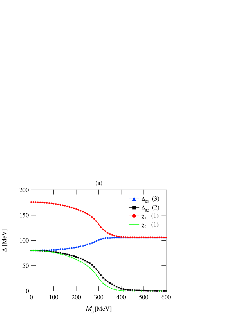
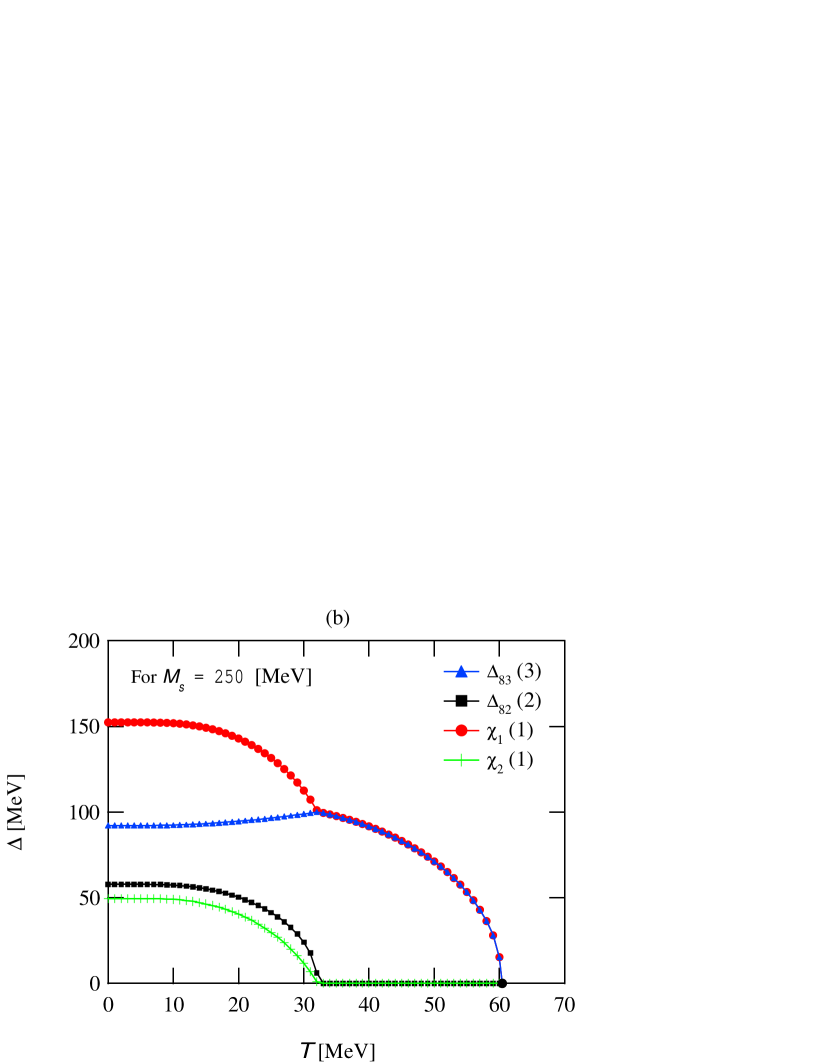
Figure 1: (a) Gaps are plotted as functions of $M_{s}$. (b) The temperature dependence of the gaps for $M_{s}=250$ MeV.

In FIG. 1(b), we display in FIG. 1, the gaps $(\Delta_{83},\Delta_{82},\chi_{1},\chi_{2})$ for $M_{s}=250$ MeV as functions of temperature. We see that as the temperature is raised, the $d$CFL phase encounters the continuous transition to the 2SC state at $T=35$MeV, and eventually the system undergoes 2nd order phase transition to the normal fermi-liquid at $T=60$MeV.

3.2 Effective potential for multi-gap parameter space

We now study how these states are realized in the multi-gap parameter space by computing the effective potential with help of the formula Eq. (16). Let us first introduce the vector

$$\vec{\Delta}(i,j)=\frac{(i-10)\vec{\Delta}_{\rm CFL}+(j-10)\vec{\Delta}_{\rm 2SC}}{50},$$ (17)

with the CFL gap vector $\vec{\Delta}_{\rm CFL}=(80,80,80,80,-175)$ and the 2SC gap vector $\vec{\Delta}_{\rm 2SC}=(106,0,-35,-50,-70)$ for $Ms=0$ (in the chiral limit). Eq. (17) define 2-dimensional planer section in the 5-dimensional gap parameter space, which includes the simple Fermi gas $(10,10)$ with $\vec{\Delta}=\vec{\bf 0}$, the CFL $(60,10)$ and the 2SC $(10,60)$. In FIG. 2, we show the contour plot of the effective potential $\Omega_{\rm eff}[\vec{\Delta}(i,j);M_{s}]$, for $M_{s}=0$ MeV (a), $200$ MeV (b), $300$ MeV (c) and $400$ MeV (d).

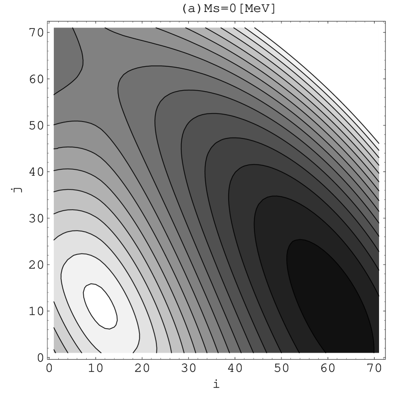
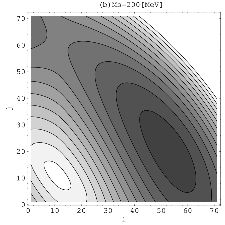
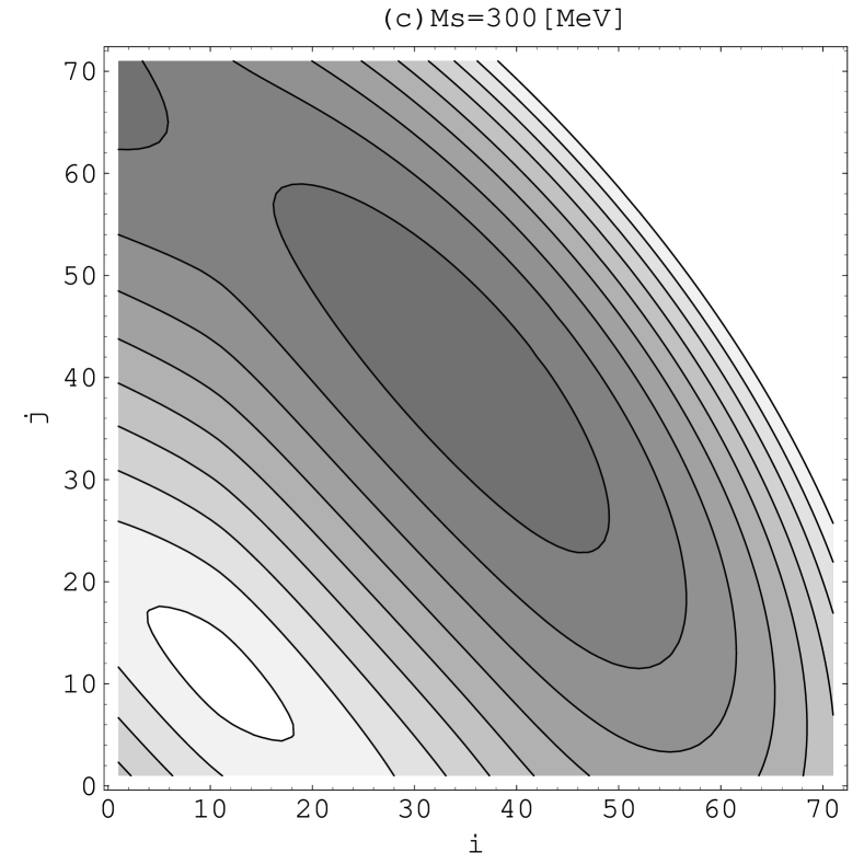
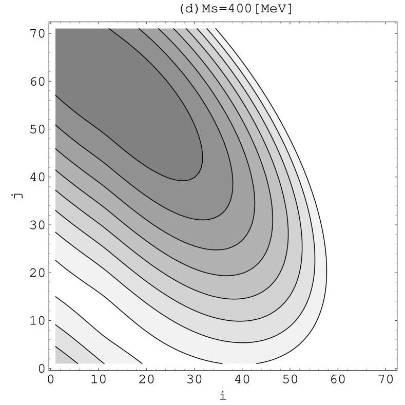
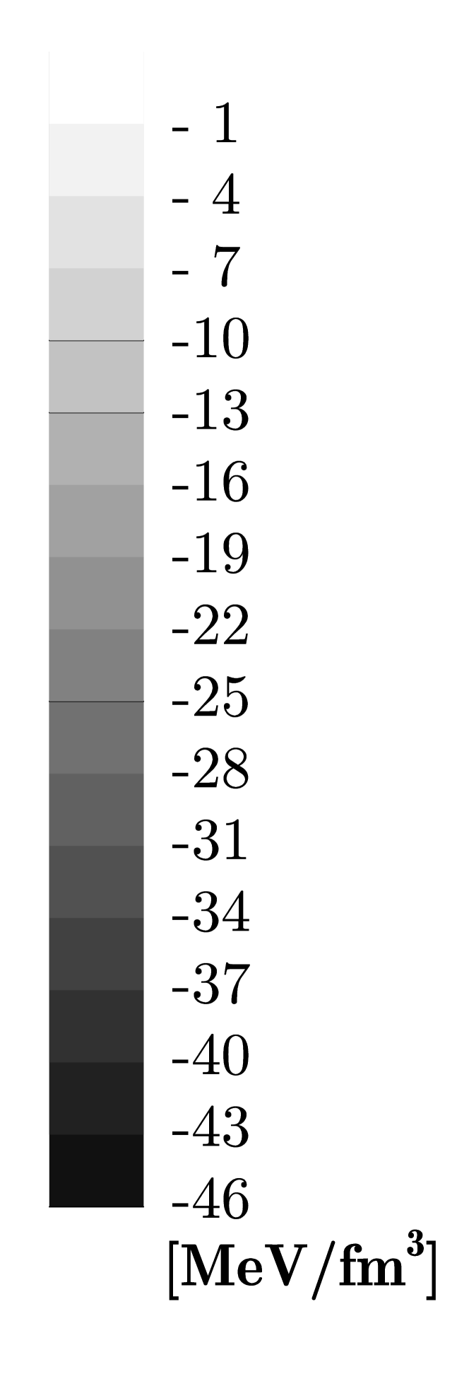
Figure 2: Contour plot of the effective potential $\Omega_{\rm eff}[\Delta(i,j)]$ where $\Delta(i,j)$ is defined by Eq. (17), for $M_{s}=0$ MeV (a), $M_{s}=200$ MeV (b), $M_{s}=300$ MeV (c), and for $M_{s}=400$ MeV (d).

We can see that the CFL state $(60,10)$ looks the global minimum in this 2-parameter space $(i,j)$ for $M_{s}=0$ MeV. On the other hand, the 2SC state $(10,60)$ is realized as a saddle point which is stable in the direction of the simple Fermi gas $(10,10)$, but is unstable in the direction towards the CFL state $(60,10)$. As the strange quark mass is increased to $200$ MeV, the CFL minimum moves towards the 2SC point, and its condensation energy gets reduced, while the position and the energy of the 2SC state is unaffected by $M_{s}$. This minimum point $(55,20)$ is expected to be located close to the distorted CFL $d$CFL state in the full 5-parameter space. The $d$CFL state gets distorted significantly towards the 2SC state at $M_{s}=300$ MeV (FIG. 2(c)), and seems absorbed into the 2SC as the strange quark mass approaches the order of the chemical potential $\sim\mu$ of the system. We can conclude that the unlocking transition is not of 1st order. More detailed analyses made in Ref. HabukiNJ reveals that this transition is of 2nd order and indicates that the $d$CFL satate at low strange quark density is the Bose-Einstein condensation of tightly bound pairs rather than the BCS state [18].

2SC as a solution of gap equation.  What should be stressed here is that the 2SC stays at least a saddle point in the full model space irrespective of the value of $M_{s}$. This means that the 2SC is always a solution of the gap equation, and if we had missed in obtaining the correct effective potential, then we misunderstood it as the true ground state instead of the $d$CFL state for intermediate strange quark mass $M_{s}$.

Unstable CFL state?  In FIG. 3(a), we plot the section of the effective potential surface FIG. 2(a) on the line linking the 2SC $(10,60)$ $\vec{\Delta}_{t=0}=\vec{\Delta}_{\rm 2SC}$ and the CFL $(60,10)$ $\vec{\Delta}_{t=1}=\vec{\Delta}_{\rm CFL}$. Both states are determined by solving the gap equation in 5-gap parameter space for $M_{s}=0$ MeV.

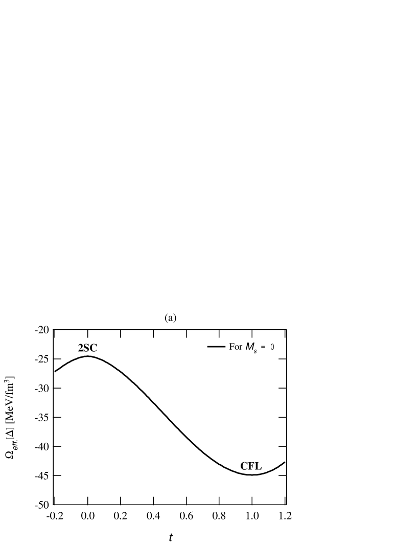
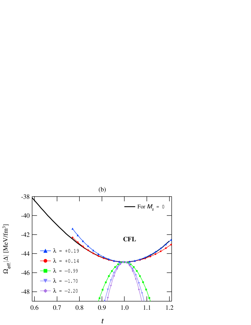
Figure 3: (a) The values of the effective potential on the 1-dimensional line connecting from the 2SC state $t=0$ to the CFL state $t=1$. (b) The bold line is just an enlargement of the potential curve for $M_{s}=0$ in (a), and five set of the points (triangles, bold dots, squares, reflected triangles, lozenges) represent the potential curves in the directions of the eigenvectors belonging to the five eigenvalues $\lambda\cong(0.19,\,0.14,\,-0.99,\,-1.70,\,-2.20)\mu^{2}$ of the Hessian curvature matrix at the CFL.

Now we address the question whether the CFL state is true global minimum even in the full model space or not. FIG. 3(b) shows us the answer for this question. Five potential curves are shown near the pure CFL for $M_{s}=0$, each of which represents the potential curve in the direction of an eigenvector belonging to the corresponding eigenvalue $\lambda$ of the Hessian curvature matrix at the CFL point $\frac{\partial^{2}\Omega}{\partial\Delta_{i}\partial\Delta_{j}}\Big{|}_{\vec{\Delta}=\vec{\Delta}_{\rm CFL}}.$ What is surprising is that the CFL state is not the global minimum in the full model space. It is unstable in three out of five directions. These three directions correspond to the color-flavor sextet channels in which the interaction acts repulsive [1]. Also it should be noted that the color-flavor sextet gap parameters do not break any symmetry, thus are not the order parameter for the unlocking as is anticipated in their critical behaviour $\sim(1-T/T_{c})^{3/2}$ near critical temperature $T_{c}$ in the chiral limit [19]. Anyway, because the effective potential becomes unbound once the sextet condensations are included, it makes no physical sense to include symmetric mean fields contribution [5, 20, 21] in the ansatz for the gap matrix. It is said that the sextet condensations are not induced within the mean field approximation, whereas they might be triggered by higher order fluctuation effects beyond the mean fields.

4 Conclusion

We have adopted the NJL model to study the phases of quark matter under high chemical potential. By making proper use of the Pauli-construction method, we have derived the exact formula for the effective potential for multi-gap parameters. In particular, we have studied the unlocking phase transition from the CFL to the 2SC. We list main results below.

1. Second order phase transition.  The unlocking transition is of continuous weak 2nd order. The 1st order unlocking never appear even at $T=0$. This contradicts the simple kinematical picture for the color-flavor unlocking transition.

2. Toughness of the CFL state.  The CFL state at $T=0$ is much more robust against the increase of $M_{s}$ than is predicted from the kinematical criterion, and the 2SC state is continuously connected from the $d$CFL state at the strange quark mass $M_{s}^{c}>\mu\,(\gg 2\sqrt{\mu\Delta_{8}(\mu,M_{s}=0)})$.

3. The 2SC as a saddle point.  2SC state is always a saddle point, a solution of the gap equation, of the effective potential for any value of $M_{s}$, which is unstable in the direction towards the $d$CFL state, as well as three color-flavor sextet directions. The $d$CFL state, a solution of the gap equation with a larger condensation energy than the 2SC state approaches the 2SC saddle point as $M_{s}$ approaches $M_{s}^{c}$.

4. Role of the sextet gap parameters.  The $d$CFL state is also unstable in the directions for three color-flavor symmetric channels. This is attributed to the fact that the interaction is repulsive in these channels. We should not include the symmetric components of the gap parameter into our ansatz from the beginning, because no Cooper instability is present in these channels due to the absence of the attractive force. However, the effects of the sextet gaps on the anti-triplet sector are very small even if they are included.

In this talk, we completely neglected the electric charge neutrality and also the color neutrality [22]. It would be interesting to include these effect into the gap equation, and to study how our $d$CFL phase is robust or fragile to be withdrawn by the neutrality condition. Also, we have ignored the usual chiral condensates in the vacuum. However, we have to include this effect to discuss the phase transitions in the lower chemical potential region. Studying phase transitions in this regime by improving our model along this line is also an interesting subject to be done in the future.

References

- [1] H. Abuki, arXiv:hep-ph/0401245.
- [2] D. Bailin and A. Love, Phys. Rep. 107, 325 (1984),
- [3] M. Iwasaki and T. Iwado, Phys. Lett. B 350, 163 (1995); M.G. Alford, K. Rajagopal and F. Wilczek, Phys. Lett. B 422, 247 (1998); R. Rapp, T. Schäfer, E.V. Shuryak and M. Velkovsky, Phys. Rev. Lett. 81, 53 (1998).
- [4] For reviews, see K. Rajagopal and F. Wilczek, arXiv:hep-ph/0011333; M.G. Alford, Ann. Rev. Nucl. Part. Sci. 51, 131 (2001); T. Schäfer, arXiv:hep-ph/0304281; D.H. Rischke, arXiv:nucl-th/0305030.
- [5] M.G. Alford, K. Rajagopal and F. Wilczek, Nucl. Phys. B 537, 443 (1999).
- [6] E. Shuster and D.T. Son, Nucl. Phys. B 573, 434 (2000); B. Park, M. Rho, A. Wirzba and I. Zahed, Phys. Rev. D 62, 034015 (2000).
- [7] T. Schäfer, Nucl. Phys. B 575, 269 (2000).
- [8] N. Evans, J. Hormuzdiar, S.D.H. Hsu and M. Schwetz, Nucl. Phys. B 581, 391 (2000).
- [9] S.D.H. Hsu, F. Sannino and M. Schwetz, Mod. Phys. Lett. A 16 1871 (2001).
- [10] D-K. Hong and S.D.H. Hsu, Phys. Rev. D 66, 071501 (2002); D-K. Hong and S.D.H. Hsu, Phys. Rev. D 68, 034011 (2003).
- [11] T. Schäfer and F. Wilczek, Phys. Rev. D 60, 074014 (1999).
- [12] M. Alford, J. Berges and K. Rajagopal, Nucl. Phys. B 558, 219 (1999).
- [13] T. Schäfer, Phys. Rev. Lett. 85, 5531 (2000);
- [14] M.G. Alford, J.A. Bowers and K. Rajagopal, Phys. Rev. D 63, 074016 (2001).
- [15] I. Shovkovy and M. Huang, Phys. Lett. B 564, 205 (2003); M. Huang and I. Shovkovy, arXiv:hep-ph/0307273.
- [16] E. Gubankova, W.V. Liu and F. Wilczek, Phys. Rev. Lett. 91, 032001 (2003); M. Alford, C. Kouvaris and K. Rajagopal, arXiv:hep-ph/0311286.
- [17] K. Iida, T. Matsuura, M. Tachibana and T. Hatsuda, arXiv:hep-ph/0312363.
- [18] M. Matsuzaki, Phys. Rev. D 62, 017501 (2000); H. Abuki, T. Hatsuda and K. Itakura, Phys. Rev. D 65, 074014 (2002).
- [19] H. Abuki, Prog. Theor. Phys. 110, 937 (2003).
- [20] I.A. Shovkovy and L.C.R. Wijewardhana, Phys. Lett. B 470, 189 (1999).
- [21] R. Casalbuoni, R. Gatto, G. Nardulli and M. Ruggieri, Phys. Rev. D 68, 034024 (2003).
- [22] K. Iida and G. Baym, Phys. Rev. D 63, 074018 (2001). M. Alford and K. Rajagopal, JHEP 0206, 031 (2002); A.W. Steiner, S. Reddy and M. Prakash, Phys. Rev. D 66, 094007 (2002); F. Neumann, M. Buballa and M. Oertel, Nucl. Phys. A 714, 481 (2003);