the twist-3 distribution amplitudes in the $B\rightarrow\pi$ transition form factor

Abstract

We derive an expression for the $B\rightarrow\pi$ transition form factor only depending the twist-3 distribution amplitudes by choosing an adequate chiral current correlator in the light-cone QCD sum rules. Our result show that the contribution from the twist-3 distribution amplitudes to the $f_{B\pi}^{+}(q^{2})$ give a constraint on the twist-3 light-cone distribution amplitude.

Key words  transition form factor, distribution amplitudes, Light-cone QCD sum rules

Heavy-to-light exclusive decays are important for understanding and testing the standard model, and it is of crucial interest to make a reliable prediction for these exclusive processes. Theoretically, the precise calculations of heavy-to-light from factors are of a great importance. Especially, it will be helpful for a clear understanding of $B\rightarrow\pi l\bar{v_{l}}(l=e,\mu)$ which provides us with a good chance to extract the CKM matrix element $|V_{ub}|$ from the available data. Recent progress on QCD factorization formula Beneke , which was proposed for $B\rightarrow\pi\pi$, $\pi$K and $\pi D$, show that the amplitudes for these nonleptonic decays can be expressed in terms of the semileptonic form factors, hadronic light-cone distribution amplitudes and hard-scattering functions that are calculated in perturbative QCD(pQCD). For the semileptonic form factors, one can take them as inputs from experimental data directly.

Many papers have tried to confront calculations of the semileptonic form factors. For example, these form factor can be calculated by pQCD Li and by applying the light-cone QCD sum rules Belyaev ; huang . In fact, a considerable long-distance contribution may dominate the heavy-light factors. The pQCD approach adapts the modified hard-scattering amplitude to them by a resummation of Sudakov logarithms, which can suppress the soft contribution beyond naive power counting. In light-cone QCD sum rules, the contribution of nonperturbative dynamics are attributed to the distribution amplitudes which are classified by their twists.

The $B\rightarrow\pi$ transition form factor were calculated in the light-cone QCD sum rules Belyaev . Remarkably, the main uncertainties in these calculations arise from light-cone distribution amplitudes which include not only the twist-2 distribution amplitude but the twist-3 and the twist-4 distribution amplitudes. The later two distribution amplitudes are understood poorly. It was shown that the contribution of the twist-3 distribution amplitudes is about 30-50$\%$ and the contribution of the twist-4 distribution amplitudes is about 5$\%$ to $B\rightarrow\pi$ transition form factor. Thus the great uncertainty, if possible, would be due to the uncertainty in the twist-3 distribution amplitudes in the framework of the light-cone QCD sum rules. In order to reduce the uncertainty Ref. huang takes an adequate chiral current correlator to make the contribution of the twist-3 distribution amplitudes vanish in the $B\rightarrow\pi$ transition form factor. Consequently, the possible pollution by them can be avoided in the $B\rightarrow\pi$ transition form factors.

It is very interesting to ask a similar question if one can derive an expression for the $B\rightarrow\pi$ transition form factor only depending the twist-3 distribution amplitudes by choosing the chiral current correlator. The answer is positive. We will discuss the question in this paper.

Let us start with the following definition of $B\rightarrow\pi$ transition form factor $f_{B\pi}^{+}(q^{2})$,

$$\langle\pi(p)|\bar{u}\gamma_{\mu}b|B(p+q)\rangle=2f_{B\pi}^{+}(q^{2})p_{\mu}+f_{B\pi}^{-}(q^{2})q_{\mu}$$ (1)

with $q$ being the momentum transfer. In order to calculate the form factor we need to construct a correlator. The different correlator gives the different expression (see Ref. Belyaev and Ref. huang ). For example, Ref.huang proposed an improved approach by choosing the chiral current and they got the transition form factor,

$$f_{B\pi}^{+}(q^{2}) =\frac{m_{0}^{2}f_{\pi}}{m_{B}^{2}f_{B}}e^{m_{B}^{2}/M^{2}}\left\{\int_{\Delta}^{1}\frac{du}{u}exp\left[-\frac{m_{b}^{2}-q^{2}(1-u)}{uM^{2}}\right]\cdot\left[\phi_{\pi}(u)-\frac{4m_{b}^{2}}{u^{2}M^{4}}g_{1}(u)\right.\right.$$ (2)

$$\left.\left.+\frac{2}{uM^{2}}\int_{0}^{u}dvg_{2}(v)\left(1+\frac{m_{b}^{2}+q^{2}}{uM^{2}}\right)\right]+\int_{0}^{1}dv\int D\alpha_{i}\frac{\theta(\alpha_{1}+v\alpha_{3}-\Delta)}{(\alpha_{1}+v\alpha_{3})^{2}M^{2}}\right.$$

$$\left.exp\left[-\frac{m_{b}^{2}-(1-\alpha_{1}-v\alpha_{3})q^{2}}{M^{2}(\alpha_{1}+v\alpha_{3})}\right]\left[2\phi_{\bot}(\alpha_{i})+2\widetilde{\phi}_{\bot}(\alpha_{i})-\phi_{\|}(\alpha_{i})-\widetilde{\phi}_{\|}(\alpha_{i})\right]\right.$$

$$\left.-4m_{b}^{2}e^{-s_{0}/M^{2}}\left[\frac{1}{(m_{b}^{2}-q^{2})^{2}}\left(1+\frac{s_{0}-q^{2}}{M^{2}}\right)g_{1}(\Delta)-\frac{1}{(s_{0}-q^{2})(m_{b}^{2}-q^{2})\frac{dg_{1}(\Delta)}{du}}\right]\right.$$

$$\left.-2e^{-s_{0}/M^{2}}\left[\frac{m_{b}^{2}+q^{2}}{(s_{0}-q^{2})(m_{b}^{2}-q^{2})}g_{2}(\Delta)-\frac{1}{m_{b}^{2}-q^{2}}\left(1+\frac{m_{b}^{2}+q^{2}}{m_{b}^{2}-q^{2}}\right)\left(1+\frac{s_{0}-q^{2}}{M^{2}}\right)\right.\right.$$

$$\left.\left.\int_{0}^{\Delta}dvg_{2}(v)\right]\right\}$$

with $D\alpha_{i}=d\alpha_{1}d\alpha_{2}d\alpha_{3}\delta(1-\alpha_{1}-\alpha_{2}-\alpha_{3})$, $m_{0}=\frac{m_{\pi}^{2}}{m_{u}+m_{d}}$ and $\Delta=(m_{b}^{2}-q^{2})/(s_{0}-q^{2})$. Here $\phi_{\pi}$ is $\pi$ meson twist-2 distribution amplitude, $g_{1}(u),g_{2}(u),\phi_{\bot}(\alpha_{i}),\widetilde{\phi}_{\bot}(\alpha_{i}),\phi_{\|}(\alpha_{i}),\widetilde{\phi}_{\|}(\alpha_{i})$ are $\pi$ meson twist-4 distribution amplitudes$,s_{0}$ is the threshold parameter which should be set to the value near the squared mass of the lowest scalar $B^{*}$ meson, and $M$ is the Borel parameter.

Now we propose to chose another chiral current to construct a correlator,

$$\Pi_{\mu}(p,q) =i\int d^{4}xe^{iq\cdot x}\langle\pi(p)|T\left\{\bar{u}(x)\gamma_{\mu}(1+\gamma_{5})b(x);\bar{b}(0)im_{b}(1-\gamma_{5})d(0)\right\}|0\rangle$$ (3)

$$=\Pi(q^{2},(p+q)^{2})p_{\mu}+\widetilde{\Pi}(q^{2},(p+q)^{2})q_{\mu},$$

which is different from that in Ref.huang . Here the chiral limit $p^{2}=m_{\pi}^{2}=0$ is made.

This correlator can be calculated in two ways. First, we discuss the hadronic representation for the correlator by inserting a complete series of intermediate state with the same quantum number as the current operator $\bar{b}~{}i(1-\gamma_{5})d$ in it. Then isolating the pole term of lowest pseudoscalar $B$ meson, we get the result,

$$\Pi_{\mu}^{H}(p,q) =\Pi^{H}(q^{2},(p+q)^{2})p^{\mu}+\widetilde{\Pi}^{H}(q^{2},(p+q)^{2})q_{\mu}$$ (4)

$$=-\frac{m_{b}\langle\pi|\bar{u}\gamma_{\mu}b|B\rangle\langle B|\bar{b}\gamma_{5}d|0\rangle}{m_{B}^{2}-(p+q)^{2}}+\Sigma_{H}\frac{m_{b}\langle\pi|\bar{u}\gamma_{\mu(1+\gamma_{5})}b|B_{H}\rangle\langle B_{H}|\bar{b}(1-\gamma_{5})d|0\rangle}{m_{B_{H}}^{2}-(p+q)^{2}}.$$

Here the intermediate states $B_{H}$ contain not only pseudoscalar resonances of the masses greater than $m_{B}$, but also scalar resonance with $J^{P}=0^{+}$, corresponding to the operator $\bar{b}d$. Substituting Eq.(1) and the definition $m_{b}\langle B|\bar{b}i\gamma_{5}d|0\rangle=m_{B}^{2}f_{B}$ into Eq.(4), the invariant amplitudes $\Pi^{H}$ and $\widetilde{\Pi}^{H}$ become

$$\Pi^{H}[q^{2},(q+p)^{2}]=\frac{-2f_{B\pi}^{+}m_{B}^{2}f_{B}}{m_{B}^{2}-(p+q)^{2}}+\int_{s_{0}}^{\infty}\frac{\rho^{H}(s)}{s-(p+q)^{2}}ds+subtraction$$ (5)

and

$$\tilde{\Pi}^{H}[q^{2},(q+p)^{2}]=\frac{-f_{B\pi}^{-}m_{B}^{2}f_{B}}{m_{B}^{2}-(p+q)^{2}}+\int_{s_{0}}^{\infty}\frac{\tilde{\rho}^{H}(s)}{s-(p+q)^{2}}ds+subtraction.$$ (6)

The terms in the integration are the contribution from higher resonances and continuum states above threshold $s_{0}$. Due to the quark-hadron duality ansatz, the spectral densities $\rho^{H}(s)$ and $\widetilde{\rho}^{H}(s)$ can be approximated by the following expression,

$$\rho^{H}(s)=\rho^{QCD}(s)\theta(s-s_{0})\quad and\quad\tilde{\rho}^{H}(s)=\tilde{\rho}^{QCD}(s)\theta(s-s_{0}).$$ (7)

On the other hand, the correlator can be calculated in QCD theory, to obtain the desired sum rule for $f_{B\pi}^{+}(q^{2})$, we work in the large space-like momentum regions $(p+q)^{2}-m^{2}_{b}\ll 0$ for the $b\bar{d}$ channel, and $q^{2}\ll m_{b}^{2}-0(1GeV^{2})$ for the momentum transfer, which correspond to the light cone region $x^{2}\simeq 0$ and are required by the validity of the operator product expansion(OPE). First we can write down a full $b$-quark propagator,

$$\langle 0\mid T{b(x)\bar{b}(0)}\mid 0\rangle = i\int\frac{d^{4}k}{2\pi}^{4}e^{ik\cdot x}\frac{\hat{k}+m_{b}}{k^{2}-m_{b}^{2}}-ig_{s}\int\frac{d^{4}k}{2\pi}^{4}e^{ik\cdot x}$$ (8)

$$\int_{0}^{1}dv\left[\frac{1}{2}\frac{\hat{k}+m_{b}}{(m_{b}^{2}-k^{2})^{2}}G^{\mu\nu}(vx)\sigma_{\mu\nu}+\frac{1}{m_{b}^{2}-k^{2}}vx_{\mu}G^{\mu\nu}(vx)\gamma_{\nu}\right],$$

where $G_{\mu\nu}$is the gluonic field strength and $g_{s}$ denote the strong-coupling constant. Carrying out the OPE for the correction and making use of Eq.(8), we require several formulas in Ref.Braun

$$\langle\pi(q)\mid\bar{u}(x)i\gamma_{5}d(0)\mid 0\rangle=\frac{f_{\pi}m_{\pi}^{2}}{m_{u}+m_{d}}\int_{0}^{1}due^{iuq\cdot x}\phi_{p}(u)$$

$$\langle\pi(q)\mid\bar{u}(x)\sigma_{\mu\nu}\gamma_{5}d(0)\mid 0\rangle=i(q_{\mu}x_{\nu}-q_{\nu}x_{\mu})\frac{f_{\pi}m_{\pi}^{2}}{6(m_{u}+m_{d})}\int_{0}^{1}due^{iuq\cdot x}\phi_{\sigma}(u)$$

$$\langle\pi(q)\mid\bar{u}(x)g_{s}G_{\mu\nu}(vx)\sigma_{\alpha\beta}\gamma_{5}d(0)\mid 0\rangle$$

$$\quad\quad\quad\quad\quad=if_{3\pi}[(q_{\mu}q_{\alpha}g_{\nu\beta}-q_{\nu}q_{\alpha}g_{\mu\beta})-(\alpha\leftrightarrow\beta)]\int D\alpha_{i}\phi_{3\pi}(\alpha_{i})e^{iq\cdot x(\alpha_{1}+v\alpha_{3})}.$$ (9)

Here $\phi_{p}(u)$ and $\phi_{\sigma}(u)$ are twist-3 distribution amplitudes of $\pi$ meson, $\phi_{3\pi}(\alpha_{i})$ is twist-3 three-particle distribution amplitude of $\pi$ meson. Substituting the above $b$-quark full propagator and the corresponding $\pi$ meson distribution amplitudes into the correlator and completing the integrations over $x$ and $k$ variables, finally we obtain an expression,

$$\Pi^{QCD}[q^{2},(p+q)^{2}] = \frac{-2f_{\pi}m_{\pi}^{2}}{m_{u}+m_{d}}\int_{0}^{1}du\frac{1}{m_{b}^{2}-(p+uq)^{2}}\left[u\phi_{p}(u)+\frac{1}{6}(2+\frac{p^{2}+m_{b}^{2}}{m_{b}^{2}-(p+uq)^{2}})\phi_{\sigma}(u)\right]$$ (10)

$$+\int_{0}^{1}dv\int D\alpha_{i}\frac{-8f_{3\pi}\phi_{3\pi}(\alpha_{i})vq\cdot p}{(m_{b}^{2}-(p+(\alpha_{1}+v\alpha_{3})q)^{2})^{2}}$$

After substituting Eq.(10) into Eq.(5) and performing the Borel transformation with respect to $(p+q)^{2}$, a sum rule for the $B\rightarrow\pi$ transition form factor can be obtained

$$f_{B\pi}^{+}(q^{2}) = \frac{m_{b}f_{\pi}}{m_{B}^{2}f_{B}}\frac{m_{\pi}^{2}}{m_{u}+m_{d}}exp[\frac{m_{B}^{2}}{M^{2}}]\left\{\int_{\Delta}^{1}duexp[-\frac{m_{b}^{2}-q^{2}(1-u)}{uM^{2}}][u\phi_{p}(u)+\frac{1}{6}(2+\frac{m_{b}^{2}+q^{2}}{uM^{2}})\phi_{\sigma}(u)]\right.$$ (11)

$$\left.-\frac{2f_{3\pi}}{f_{\pi}}\frac{m_{u}+m_{d}}{m_{\pi}^{2}}\int_{0}^{1}dv\int D\alpha_{i}\frac{\theta(\alpha_{1}+v\alpha_{3}-\Delta)}{(\alpha_{1}+v\alpha_{3})^{2}}exp[-\frac{m_{b}^{2}-q^{2}(1-\alpha_{1}-v\alpha_{3})}{(\alpha_{1}+v\alpha_{3})M^{2}}]\right.$$

$$\left.\cdot[1-\frac{m_{b}^{2}-q^{2}}{(\alpha_{1}+v\alpha_{3})M^{2}}]\phi_{3\pi}(\alpha_{i})\right\},$$

where M is the Borel parameter. Eq.(11) shows that $f_{B\pi}^{+}(q^{2})$ only depends on the twist-3 distribution amplitudes. It means that the contribution from the twist-3 distribution amplitudes to the $f_{B\pi}^{+}(q^{2})$ has the same order of magnitude as that from the leading twist distribution amplitude.

Now we need to make a choice of input parameters entering the sum rule Eq.(11) for $f_{B\pi}^{+}(q^{2})$. Let us specify the twist-3 model of the pion distribution amplitudes, $\phi_{p}(u)$ ,$\phi_{\sigma}(u)$ and $\phi_{3\pi}(\alpha_{i})$(Ref.Belyaev ; Braun ),

$$\phi_{p}(u)=1+B_{2}\frac{1}{2}(3(2u-1)^{2}-1)+B_{4}\frac{1}{8}(35(2u-1)^{4}-30(2u-1)^{2}+3),$$

$$\phi_{\sigma}(u)=6u(1-u)\left[1+C_{2}\frac{3}{2}(5(2u-1)^{2}-1)+C_{4}\frac{15}{8}(21(2u-1)^{4}-14(2u-1)^{2}+1)\right]$$

and

$$\phi_{3\pi}(\alpha_{i})=360\alpha_{1}\alpha_{2}\alpha_{3}^{2}$$

$$\quad\quad\quad\quad\left[1+\varpi_{1,0}\frac{1}{2}(7\alpha_{3}-3)+\varpi_{2,0}(2-4\alpha_{1}\alpha_{2}-8\alpha_{3}+8\alpha_{3}^{2})+\varpi_{1,1}(3\alpha_{1}\alpha_{2}-2\alpha_{3}+3\alpha_{3}^{2})\right],$$

where $B_{2}=30R$, $B_{4}=\frac{3}{2}(4\varpi_{2,0}-\varpi_{1,1}-2\varpi_{1,0})$, $C_{2}=R(5-\frac{1}{2}\varpi_{1,0})$, $C_{4}=\frac{1}{10}R(4\varpi_{2,0}-\varpi_{1,1})$ with $R=\frac{f_{3\pi}}{m_{0}f_{\pi}}$, $f_{\pi}=133MeV$, $f_{3\pi}=0.0026GeV^{2}$ and $\varpi_{1,0}=-2.18$, $\varpi_{2,0}=8.12$, $\varpi_{1,1}=-2.59$. Other input parameters are taken in the following: $s_{0}=33GeV^{2}$, $M^{2}=16GeV^{2}$, $m_{b}=4.7GeV$, $m_{B}=5.28GeV$ and $f_{B}=165MeV$. With these inputs, we ca carry out the numerical analysis. The form factor Eq.(11) in this paper is depicted by the solid curve in Fig.1. The dashed and dotted curves in Fig.1 are taken from Ref.Belyaev and Ref.huang respectively. It shows that three curves are consistent in the region $q^{2}<16GeV^{2}$. In fact, the applicability of the light cone QCD sum rules is questionable as $q^{2}\geqslant 18GeV^{2}$ huang , and a comparison between the different approaches in the regions is meaningless. Also one can see from Fig.1 that the form factor go up very quickly beyond the region $q^{2}=15GeV^{2}$ as long as the twist-3 distribution amplitudes make contribution to sum rules.

In summary, we show that the different expressions for the $B\rightarrow\pi$ transition form factor by choosing the different adequate current correlator in the light cone QCD sum rules. Especially, we derive the expression for $f_{B\pi}^{+}(q^{2})$ only depending the twist-3 distribution amplitudes. It is consistent with other expressions by employing the present model for the pion distribution amplitudes. Conversely, they provide constraints on the pion distribution amplitudes.

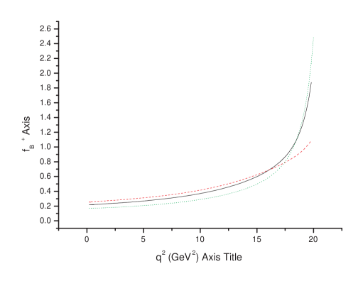
Figure 1: The transition form factor $f_{B\pi}^{+}(q^{2})$ in the light cone QCD sum rules at $M^{2}=16GeV^{2}$ with $s_{0}=33GeV^{2}$, $m_{b}=4.7GeV$, $m_{B}=5.28GeV$, $f_{B}=165MeV$, $f_{\pi}=132MeV$.

References

• (1) M.Beneke, G.Buchalla, M.Neubert and C.T.Sachrajda, Phys.Rev.Lett.83,1914(1999); Nucl.Phys.B591,313(2000);
M.Beneke and M.Neubert, Nucl.Phys.B675:333-415,2003; hep-ph/0308039.
• (2) H.N.Li and H.L.Yu, Phys.Rev.Lett.74,4388(1995).
• (3) V.M.Belyaev, A.Khodjamirian and R.RΓΌckl,Z.Phys.C60, 349(1993);
V.M.Belyaev, V.M.Braun, A.Khodjamirian and R.RΓΌckl, Phys.Rev.D51, 6177(1995).
• (4) Tao Huang, Zuo Hong Li and Xiang Yao Wu, Phys.Rev.D63, 094001(2001);
Zhi-Gang Wang, Ming-Zhen Zhou and Tao Huang, Phys.Rev.D67:094006,2003.
• (5) V.M.Braun and I.E.Filyanov, Z.Physik C 48(1900)239.