LBNL-54488

SN-ATLAS-2004-038

Exploring Little Higgs Models with ATLAS at the LHC

G. Azuelos^a, K. Benslama^a, D. Costanzo^b, G. Couture^a J.E. Garcia^c, I. Hinchliffe^b, N. Kanaya^d, M. Lechowski^e, R. Mehdiyev^a,f G. Polesello^g, E. Ros^c, D. Rousseau^e

^aU. of Montreal, Montreal, Canada

^bLawrence Berkeley National Laboratory, Berkeley, CA

^cIFIC, University of Valencia/CSIC, Spain

^d University of Victoria, Victoria, BC, Canada

^e University of Paris-Sud, IN2P3-CNRS, Orsay, France

^fInstitute of Physics, Academy of Sciences of Azerbaijan, Baku, Azerbaijan

^gINFN, Sezione di Pavia, Pavia, Italy

We discuss possible searches for the new particles predicted by Little Higgs Models at the LHC. By using a simulation of the ATLAS detector, we demonstrate how the predicted quark, gauge bosons and additional Higgs bosons can be found and estimate the mass range over which their properties can be constrained.

1 Introduction

Recently, new models have been proposed as possible solutions to the hierarchy problem of the Standard Model. This problem, also referred to as the fine-tuning problem, is most easily phrased as follows. If radiative corrections to the Higgs mass are computed using an ultra-violet cut off $\Lambda$, the resulting value of the Higgs mass is of order $\Lambda$ unless there is a very delicate cancellation. The “Little Higgs” models  [1, 2] provide just enough new physics to generate cancellations and preserve a light Higgs boson while raising the ultra-violet cut off to a scale of several tens of TeV where constraints on new particles from existing experiments are very weak. In the Standard Model, there are three contributions to radiative corrections to the Higgs mass that dominate the hierarchy problem. In order of importance they are the top quark, the electro-weak gauge bosons, and the Higgs itself. If the loop integrals are cut off at scale $\Lambda=10$ TeV, these corrections are:

• from the top loop $\delta m_{h}^{2}=\frac{3}{8\pi^{2}}\lambda_{t}^{2}\Lambda^{2}\sim(2\hbox{ TeV})^{2}$;

• from the $W/Z$ loops $\delta m_{h}^{2}\sim\alpha_{w}\Lambda^{2}\sim-(750\hbox{ GeV})^{2}$;

• from the Higgs loop $\delta m_{h}^{2}\sim\frac{\lambda}{16\pi^{2}}\Lambda^{2}\sim-(1.25m_{h})^{2}$.

The “Little Higgs” models implement the idea that the Higgs boson is a pseudo-Goldstone boson  [3, 4]. They are constructed by embedding the Standard Model inside a larger group with an enlarged symmetry. The larger symmetry is then broken at some high scale $\Lambda_{H}=4\pi f$, so that the Higgs mass is protected from radiative corrections at one loop that are dependent quadratically on $\Lambda_{H}$. From a phenomenological point of view, the effect of this symmetry is to require the existence of new particles whose couplings ensure that the large contributions to the Higgs mass are canceled. There must be three types of new particles corresponding to the three contributions listed above. In this paper we study the observability, using the ATLAS detector at the LHC, of these new particles. For definiteness we will use the “Littlest Higgs” model  [5, 6] although many of our results can be reinterpreted in other models. In this model, a new charge 2/3 quark, $T$, which is an electroweak singlet is predicted. It mixes with the top quark and decays via this mixing to $Wb$, $th$ and $tZ$ final states. Since this particle is canceling the largest contribution to the Higgs mass, its mass cannot be too large or the fine tuning problem will reappear: $m_{T}<2\hbox{ TeV}(\frac{m_{h}}{200\hbox{ GeV}})^{2}$  [5]. The model is based on an extended gauge group containing the gauged subgroup $[SU(2)_{1}\otimes U(1)_{1}]\otimes[SU(2)_{2}\otimes U(1)_{2}]$ which itself implies, in addition to the $W$, $Z$ and $\gamma$ of the Standard Model, four new gauge bosons $W_{H}^{\pm}$, $A_{H}$ and $Z_{H}$. Since these new gauge bosons are canceling the contributions from $W/Z$ loops, their masses are less strongly constrained: $M_{W_{H}}<6\hbox{ TeV}(\frac{m_{h}}{200\hbox{ GeV}})^{2}$. The model also predicts new Higgs particles forming an $SU(2)_{L}$ triplet ($\phi$) which contains a doubly charged state. As the Higgs contribution to the fine-tuning problem is the smallest, these masses are the least constrained: $m_{\phi}<10$ TeV.

Precision electroweak data severely constrain the model considered here  [7, 8]. We will not take these constraints into account as they can be avoided in other models whose LHC phenomenology is similar to the one we consider  [9, 10].

The rest of this paper is organized as follows. We discuss the channels available for the discovery and measurement of the properties of the $T$ quark in the next section. We then discuss the new gauge bosons and the doubly charged Higgs boson and finally we draw some conclusions regarding the LHC sensitivity to Little Higgs models. Specific masses are chosen for the the simulations shown below. Our main purpose is to assess the potential of ATLAS for the Little Higgs Model, so we have chosen masses that are rather large as observation is more difficult in these cases due to the smaller event rates. In a few cases where we were concerned that the signal to background ratio might get worse with reduced masses, we show a lower mass case to allay this concern. A Higgs mass of 120 GeV was assumed and we comment on the effect of this choice in the conclusion. We further assume that the Higgs boson has been discovered and that its mass is known.

PYTHIA 6.203  [11] with suitably normalized rates was used to generate events which were passed through the ATLAS fast simulation [12] which provides a parametrized response of the ATLAS detector to jets, electrons, muons, isolated photons and missing transverse energy. This fast simulation has been validated using a large number of studies  [13] where it was compared with, and adjusted to agree with, the results of a full, GEANT based, simulation  [14]. The performance for high luminosity environment is assumed. The fast simulation provides a standard definition of isolated leptons and photons that is used throughout. Using these definitions, fake electrons arising from misidentified jets are negligible for our purposes. Jets are reconstructed using a cone algorithm with a cone of size $\Delta R=0.4$. Performance for the high luminosity ($10^{34}$ cm^-2 sec^-1 is assumed. There is one case, that of identifying jets containing $b-$hadrons ($b-$tagging), where the validation was in a kinematic range different from that needed in this study. In this case, a full simulation was performed and its results used to reparametrize the tagging efficiency and the rejection against non$-b$ jets used in fast simulation. (See details in Section 3.3.) The event selections are based on the characteristics of the signal being searched for, and are such that they will pass the ATLAS trigger criteria. The most important triggers arise from the isolated leptons, jets or photons present in the signal. These event selections exploit the experience gained in devising the stratgies for other new physics searches  [13]. The selections have not been optimized in detail for the particular cases under study. In some cases, the cuts have been varied when the particle masses were changed; for example raising the threshold on particular physics objects as the mass of the new particle increases. It is not claimed that the event selections are optimal. Detailed optimization is not wise at this stage due to uncertainties in the background estimates.

PYTHIA was also use for simulation of the backgrounds. In a few cases, discussed explicitly below, other event generators were used if the backgrounds are needed in regions of phase space where PYTHIA is known to be less reliable (mainly for processes with large numbers of well-separated jets). Systematic uncertainties in the level of the backgrounds are, in many cases, difficult to estimate. Since we are only interested in the observability of the signals, but are not, at this stage, attempting to evaluate the precision with which cross-sections can be measured, these uncertainties are not expected to affect significantly the results. Indeed, in most cases, the signals appear as clear peaks above a smooth background. The precision with which masses can be measured will ultimately depend on the calibration of the detector. Previous studies can be consulted for a discussion of these issues  [13].

2 Search for $T$ and determination of its properties

The $T$ quark can be produced at the LHC via two mechanisms: QCD production via the processes $gg\to T\overline{T}$ and $q\overline{q}\to T\overline{T}$ which depend only on the mass of $T$; and production via $W$ exchange $qb\to q^{\prime}T$ which leads to a single $T$ in the final state and therefore falls off much more slowly as $m_{T}$ increases. This latter process depends on the model parameters and, in particular, upon the mixing of the $T$ with the conventional top quark. The Yukawa couplings of the new $T$ are given by two constants $\lambda_{1}$ and $\lambda_{2}$

$$\lambda_{1}(i{Qht_{r}}+f{T_{L}t_{r}}-\frac{1}{2f}{T_{L}t_{r}hh^{\dagger}})+\lambda_{2}f({T_{L}T_{R}})$$

where $h$ is the Standard Model Higgs doublet, $Q$ is a doublet containing the left-handed top and bottom quarks ($t_{L}$, $b_{L}$), and $t_{R}$ is the right-handed top quark; (for details see  [15] whose notation is followed here). The physical top quark mass eigenstate is a mixture of $t$ and $T$. These couplings contain three parameters $\lambda_{1}$, $\lambda_{2}$ and $f$ that determine the masses of $T$ and the top quark as well as their mixings. Two of the parameters can be reinterpreted as the top mass and the $T$ mass. The third can then be taken to be $\lambda_{1}/\lambda_{2}$. This determines the mixings and hence the coupling strength $TbW$ which controls the production rate via the $qb\to q^{\prime}T$ process. The production rates are shown in Figure 1 from  [15]. It can be seen that single production dominates for masses above 700 GeV. As we expect that we are sensitive to masses larger than this, we consider only the single production process in what follows. We assume the following cross-sections: for $m_{T}=0.7,1.0,1.3,1.6$ TeV, $\sigma=1000,200,45,12$ ${\rm fb}$ for $\lambda_{1}/\lambda_{2}=1$. Events generated using PYTHIA were normalized to these values.

The decay rates of $T$ are as follows

$$\Gamma(T\to tZ)={1\over 2}\Gamma(T\to bW)=\Gamma(T\to th)={\kappa^{2}\over 32\pi}M_{T}$$

with $\kappa={\lambda_{1}^{2}/\sqrt{\lambda_{1}^{2}+\lambda_{2}^{2}}}$ implying that $T$ is a narrow resonance. The last of these decays would be expected for a charged 2/3 4^th generation quark; the first two are special to the “Little Higgs Model”. We now discuss the reconstruction in these channels.

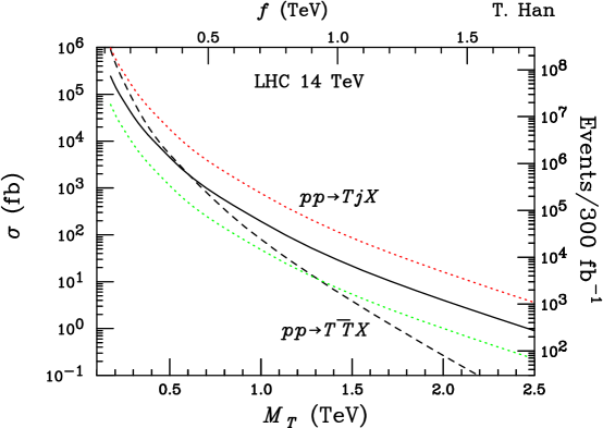
Figure 1: Figure showing the production rate of the $T$ quark at the LHC as a function of its mass  [15]. The heavy dashed line shows the pair production and the solid and two dotted lines the single production rate for three value of $\lambda_{2}/\lambda_{1}$; from highest to lowest $\lambda_{2}/\lambda_{1}=2,1,0,5$. (We are grateful to T. Han for providing this figure.)

2.1 $T\to Zt$

This channel can be observed via the final state $Zt\to\ell^{+}\ell^{-}\ell\nu b$, which implies that the events contain three isolated leptons, a pair of which reconstructs to the $Z$ mass, one $b-$jet and missing transverse energy. The background is dominated by $WZ$, $ZZ$ and $tbZ$. The last cannot be simulated using PYTHIA, and was therefore generated using CompHep  [16]. Events were selected as follows.

• Three isolated leptons (either $e$ or $\mu$) with $p_{T}>$ 40 GeV and $\left|\eta\right|<2.5$. One of these is required to have $p_{T}>$ 100 GeV.

• No other leptons with $p_{T}>$ 15 GeV.

• $\hbox to0.0pt{\hbox to7.95831pt{\hfil/\hfil}\hss}E_{T}>100$ GeV.

• At least one tagged $b-$jet with $p_{T}>$ 30 GeV.

The presence of the leptons ensures that the events are triggered. A pair of leptons of same flavor and opposite sign is required to have an invariant mass within 10 GeV of $Z$ mass. The efficiency of these cuts is 3.3% for $m_{T}=1000$ GeV. The third lepton is then assumed to arise from a $W$ and the $W$’s momentum reconstructed using it and the measured $\hbox to0.0pt{\hbox to7.95831pt{\hfil/\hfil}\hss}E_{T}$.

The invariant mass of the $Zt$ system can then be reconstructed by including the $b-$jet. This is shown in Figure 2 for $m_{T}=1000$ GeV where a clear peak is visible above the background. Following the cuts, the background is dominated by $tbZ$ which is more than 10 times greater than all the others combined. The cuts accept 0.8% of this background  [17].

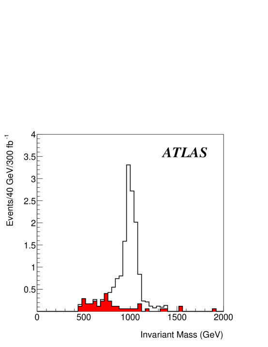
Figure 2: Reconstructed mass of the $Z$ and $t$ (inferred from the measured lepton, $\hbox to0.0pt{\hbox to7.95831pt{\hfil/\hfil}\hss}E_{T}$, and tagged $b-$jet). The signal $T\to Zt$ is shown for a mass of 1000 GeV. The background, shown as the filled histogram, is dominated by $WZ$ and $tbZ$ (the latter is larger) production. The signal event rates correspond to $\lambda_{1}/\lambda_{2}=1$ and a $BR(T\to ht)$ of 25%. More details can be found in Ref  [17].

Using this analysis, the discovery potential in this channel can be estimated. The signal to background ratio is excellent as can be seen from Figure 2. Requiring a peak of at least $5\sigma$ significance containing at least 10 reconstructed events implies that for $\lambda_{1}/\lambda_{2}=1(2)$ and 300 fb^-1 the quark of mass $M_{T}<1050(1400)$ GeV is observable. At these values, the single $T$ production process dominates, justifying a posteriori the neglect of $T\overline{T}$ production in this simulation.

2.2 $T\to Wb$

This channel can be reconstructed via the final state $\ell\nu b$. The following event selection was applied.

• At least one charged lepton with $p_{T}>$100 GeV.

• One $b$-jet with $p_{T}>$ 200 GeV.

• No more than 2 jets with $p_{T}>30$ GeV.

• Mass of the pair of jets with the highest $p_{T}$ is greater than $200$ GeV.

• $\hbox to0.0pt{\hbox to7.95831pt{\hfil/\hfil}\hss}E_{T}>$100 GeV.

The lepton provides a trigger. The efficiency of this selection for a $T$ of mass 1 TeV is 14%. The backgrounds arise from $t\overline{t}$, single top production and QCD production of $Wb\overline{b}$. These are estimated using PYTHIA for the first one, CompHep  [16] for the second and AcerMC  [18] for the last. The requirement of only one tagged $b-$jet and the high $p_{T}$ lepton are effective against all of these backgrounds. The requirement of only two energetic jets is powerful against the dangerous $t\overline{t}$ source where the candidate $b-$jet arises from the $t$ and the lepton from the $\overline{t}$. These cuts reduce the total $t\overline{t}$ and $Wb\overline{b}$ by factors of $2.5\times 10^{-5}$ and $7.5\times 10^{-5}$ respectively. Figure 3 shows the reconstructed mass of the $Wb$ system where the $W$ momentum is inferred from the measured lepton $\hbox to0.0pt{\hbox to7.95831pt{\hfil/\hfil}\hss}E_{T}$ using the $W$ mass as a constraint. The plot shows the signal arising from $T$ of mass 1 TeV as a peak over the remaining background. The signal to background ratio is somewhat worse than in the previous case primarily due to the $t\overline{t}$ contribution.

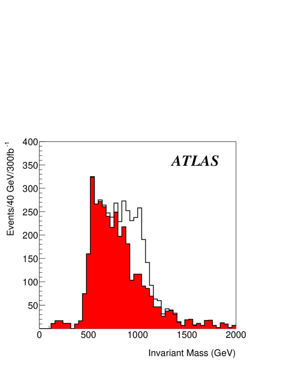
Figure 3: Reconstructed mass of the $W$ (inferred from the measured lepton and $\hbox to0.0pt{\hbox to7.95831pt{\hfil/\hfil}\hss}E_{T}$) and tagged $b-$jet. The signal arises from the decay $T\to Wb$ and is shown a for mass of 1000 GeV. The background, shown separately as the filled histogram, is dominated by $t\overline{t}$ and single top production (the former is larger). The signal event rates correspond to $\lambda_{1}/\lambda_{2}=1$ and a $BR(T\to Wb)$ of 50%. More details can be found in Ref  [17].

From this analysis, the discovery potential in this channel can be estimated. For $\lambda_{1}/\lambda_{2}=1(2)$ and 300 fb^-1 $M_{T}<2000(2500)$ GeV has at least a $5\sigma$ significance.

2.3 $T\to ht$

In this final state, the event topology depends on the Higgs mass. For a Higgs mass of 120 GeV the decay to $b\overline{b}$ dominates. The semileptonic top decay $t\to Wb\to\ell\nu b$ produces a lepton that can provide a trigger. The final state containing of an isolated lepton and several jets then needs to be identified. The initial event selection is as follows.

• One isolated $e$ or $\mu$ with $p_{T}>$ 100 GeV and $\left|\eta\right|<2.5$.

• Three jets with $p_{T}>$ 130 GeV.

• At least one jet tagged as a $b-$jet.

The dijet mass distribution of all pairs of jets in events from $T$ production that pass these cuts is shown in Figure 4. A clear peak at the Higgs mass is visible. It should be noted that the jets in this plot are not required to be tagged as $b-$jets. The requirement of more than one jet tagged as a $b-$jet lowers the efficiency and is not necessary to extract a signal. Events were further selected by requiring that at least one di-jet combination have a mass in the range 110 to 130 GeV. If there is a pair of jets with invariant mass in the range 70 to 90 GeV, the event is rejected; this will help to reduce the $t\overline{t}$ background. The measured missing transverse energy and the lepton were then combined using the assumption that they arise from a $W\to\ell\nu$ decay. Events that are consistent with this are retained and the $W$ momentum inferred. The invariant mass of the reconstructed $W$, $h$ and one more jet is formed and the result shown in Figure 5. For a mass of 1000 GeV, the cuts accept 2.3% of the signal events. The width of the reconstructed $T$ resonance is dominated by experimental resolution.

The signal shown in Figure 5 assumes that $\lambda_{1}/\lambda_{2}=1$. The background is dominated by $t\overline{t}$ events as a semileptonic decay of either $t$ or $\overline{t}$ produces all objects necessary to pass the event selection. Only the different kinematics in the signal and background can distinguish them. For example, the lighter top quark implies that the lepton has a softer $p_{T}$ spectrum than that from the signal. The larger background implies that discovery in this mode is more difficult than the cases discussed above. However once the $T$ has been discovered in another channel, the peak shown in Figure 5, which has a significance above $4\sigma$ that is sufficient to confirm a signal and constrain the branching ratio.

As the mass is reduced towards the top mass, the signal becomes more difficult to extract from the $t\overline{t}$ background as the leptons and jets from the $T$ decay become softer. In order to investigate this posssible difficulty, a $T$ mass of 700 GeV was simulated. The cuts on the jets and leptons must be relaxed, to 90 GeV for the jets and to 70 GeV for the lepton. With these values, the signal efficiency is only reduced to 1.1%. Figure 6 shows the resulting distribution. The larger background results in a less significant signal. The signal shown is approximately $3\sigma$ significance which will not provide a discovery, but would confirm a signal seen in another channel and will enable a constraint on the couplings to be deduced. Of course, a larger value of $\lambda_{1}/\lambda_{2}$ will result in a clearer signal.

Figure 4: Plot showing the dijet mass distribution arising from the decay $T\to ht$. All combinations of jets are shown.

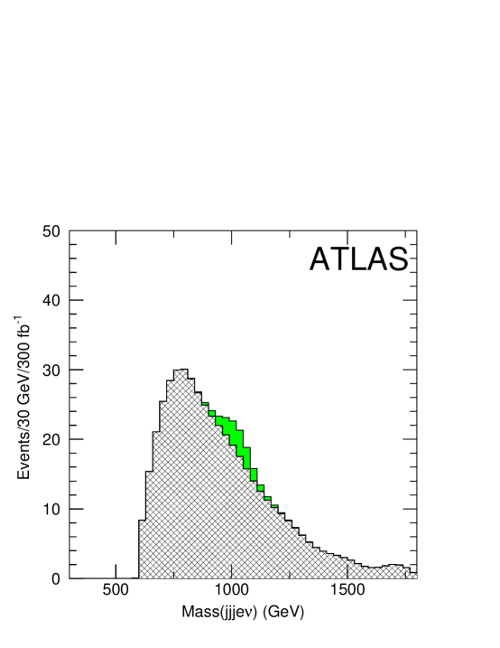
Figure 5: Reconstructed mass of the $W$ (inferred from the isolated lepton and missing transverse energy) and three jets, two of which are required to have an invariant mass consistent with the Higgs mass. The signal arises from the decay $T\to ht$ and is shown for a mass of 1000 GeV. The background, shown in cross-hatching, is dominated by $t\overline{t}$ production. The signal event rates correspond to $\lambda_{1}/\lambda_{2}=1$ and a $BR(T\to ht)$ of 25%.

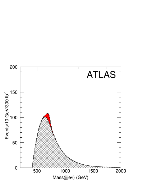
Figure 6: As for Figure 5 except that the $T$ mass is 700 GeV and the cuts are looser (see text).

3 Search for new gauge bosons

The model predicts the existence of one charged $W_{H}$ and two neutral ($Z_{H}$ and $A_{H}$) heavy gauge bosons. $W_{H}$ and $Z_{H}$ are almost degenerate in mass and are typically heavier than $A_{H}$. All these bosons are likely to be discovered via their decays to leptons. However, in order to distinguish these gauge bosons from those that can arise in other models, the characteristic decays $Z_{H}\to Zh$ and $W_{H}\to Wh$ must be observed  [19]. The properties of the new gauge bosons are determined by the couplings of the gauge theory $[SU(2)_{1}\otimes U(1)_{1}]\times[SU(2)_{2}\otimes U(1)_{2}]$ implying two couplings in addition to those of the Standard Model $[SU(2)_{L}\otimes U(1)]$ group. These additional parameters can be taken to be two angles $\theta$ and $\theta^{\prime}$ (somewhat analogous to $\theta_{W}$ of the Standard Model). Once the masses of the new bosons are specified, $\theta$ determines the couplings of $Z_{H}$ and $\theta^{\prime}$ those of $A_{H}$ (if it is assumed that there are no anomalies). In the case of $Z_{H}$, the branching ratio into $e^{+}e^{-}$ and $\mu^{+}\mu^{-}$ rises with $\cot\theta$ to an asymptotic value of 4%.

3.1 Discovery of $Z_{H}$ and $A_{H}$

A search for a peak in the invariant mass distribution of either $e^{+}e^{-}$ or $\mu^{+}\mu^{-}$ is sensitive to the presence of $A_{H}$ or $Z_{H}$. As an example, Figure 7 shows the $e^{+}e^{-}$ mass distribution arising from a $Z_{H}$ of mass of 2 TeV for $\cot\theta=1$ and $\cot\theta=0.2$. The production cross-section for the former (latter) case is 1.2 (0.05) pb  [15]. Events were required to have an isolated $e^{+}$ and $e^{-}$ of $p_{T}>20$ GeV and $\left|\eta\right|<2.5$ which provides a trigger. The Standard Model background shown on the plot arises from the Drell-Yan process. In order to establish a signal we require at least 10 events in the peak of at least $5\sigma$ significance. Figure 8 shows the accessible region as a function of $\cot\theta$ and $M_{Z_{H}}$; a slightly greater reach can be obtained by including the $\mu^{+}\mu^{-}$ channel. Except for very small values of $\cot\theta$, where the leptonic branching ratio is very small, the reach covers the entire region expected in the model. A similar search for $A_{H}$ can be carried out and the accessible region as a function of $\tan\theta^{\prime}$ and $M_{A_{H}}$ is shown in Figure 9. Masses greater than 3 TeV are not shown as these are not allowed in the model. There is a small region around $\tan\theta^{\prime}\sim 1.3$ where the branching ratio to $\mu^{+}\mu^{-}$ and $e^{+}e^{-}$ is very small and the channel is insensitive.

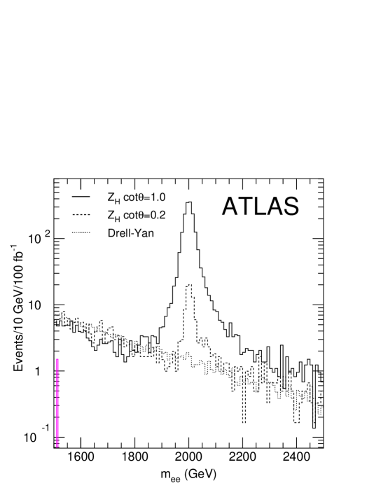
Figure 7: Plot showing the $e^{+}e^{-}$ mass distribution arising from a $Z_{H}$ of mass of 2 TeV for $\cot\theta=1$ (upper, solid, histogram) and $\cot\theta=0.2$ (middle, dashed, histogram). The lowest, dotted. histogram shows the distribution from background only.

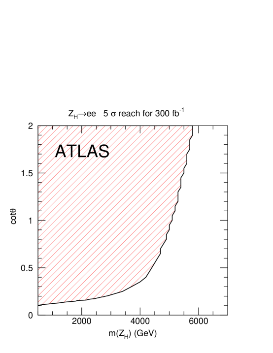
Figure 8: Plot showing the accessible region (shaded) in the channel $Z_{H}\to e^{+}e^{-}$ as a function of the mass and the mixing $\cot\theta^{\prime}$.

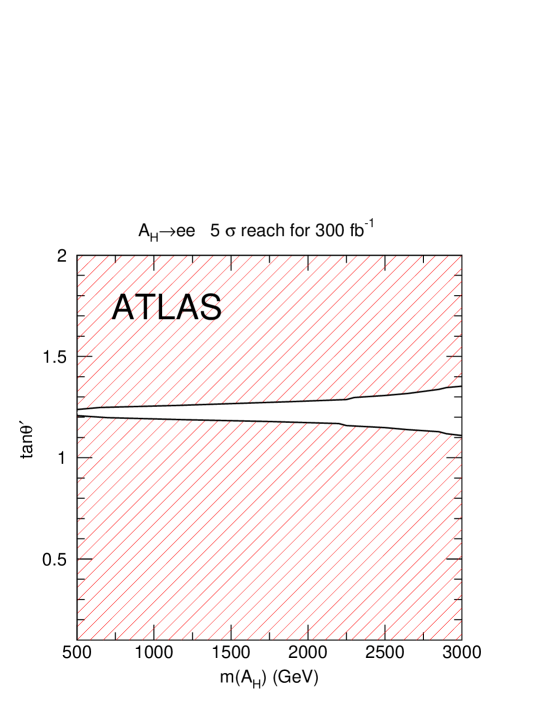
Figure 9: Plot showing the accessible region (shaded) in the channel $A_{H}\to e^{+}e^{-}$ as a function of the mass and the mixing $\tan\theta^{\prime}$. significance.

3.2 Discovery of $W^{\pm}_{H}$

The decay $W^{\pm}_{H}\to\ell\nu$ manifests itself via events that contain an isolated charged lepton and missing transverse energy. Events were selected by requiring an isolated electron with $e^{-}$ or $e^{+}$ of $p_{T}>200$ GeV, $\left|\eta\right|<2.5$ and $\hbox to0.0pt{\hbox to7.95831pt{\hfil/\hfil}\hss}E_{T}>200$ GeV. The transverse mass from $\hbox to0.0pt{\hbox to7.95831pt{\hfil/\hfil}\hss}E_{T}$ and the observed lepton is formed and the signal appears as a peak in the distribution as illustrated in Figure 10. There is a small background from $t\overline{t}$ events as can be seen from the plot; the main background arises from $\ell\nu$ production via a virtual $W$, labeled as Drell-Yan on the figure. In order to establish a signal we require at least 10 events in the signal region of at least $5\sigma$ significance. Figure 11 shows the accessible region as a function of $\cot\theta$ and $M_{W_{H}}$; a slightly greater reach can be obtained by including the $\mu\nu$ channel. Except for very small values of $\cot\theta$, the reach covers the region allowed in the model.

Figure 10: Plot showing the transverse mass distribution from $\hbox to0.0pt{\hbox to7.95831pt{\hfil/\hfil}\hss}E_{T}$ and $e$ arising from a $W_{H}$ of mass 2 TeV for $\cot\theta=0.5$ (upper histogram) and $\cot\theta=0.2$ (second highest histogram). The third highest histogram shows shows the distribution from the Drell-Yan background. The very small background from $t\overline{t}$ is also shown.

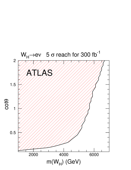
Figure 11: Plot showing the accessible region (shaded) in the channel $W_{H}\to\ell\nu$ as a function of the mass and the mixing $\cot\theta$.

3.3 Measurement of $Z_{H}\to Zh$, $A_{H}\to Zh$ and $W_{H}\to Wh$

Observation of the cascade decays $Z_{H}\to Zh$, $A_{H}\to Zh$, and $W_{H}\to Wh$ provides crucial evidence that an observed new gauge boson is of the type predicted in the Little Higgs Models. We begin by discussing $Z_{H}\to Zh$  [20]. For our choice of Higgs mass, the decay $Zh\to\ell^{+}\ell^{-}b\overline{b}$ results in a final state with two $b-$jets that reconstruct to the Higgs mass and a $\ell^{+}\ell^{-}$ pair that reconstructs to the $Z$ mass. The coupling $Z_{H}Zh$ is proportional to $\cot 2\theta$. When combined with the coupling of $Z_{H}$ to quarks that controls the production cross-section, the $\cot\theta$ dependence of the rate in this channel is shown in Figure 12, which illustrates the difficulty of observation when $\cot\theta\sim 1$.

The transverse momentum of the $b-$jets from this Higgs decay is of order $0.25M_{Z_{H}}$ since the Higgs is boosted. This is larger than the $p_{T}$ of the jets in the full simulation samples of $Wh$ events  [13] that were used for parameterizing the fast simulation. The average transverse momentum of the $h$ is of order its mass in the $Wh$ sample. Therefore a full, GEANT based  [14], simulation was run and the events reconstructed to check the $b-$tagging assumptions in the fast simulation. A sample of events arising from $Z_{H}$ of mass 2 TeV decaying to $Zh$ was produced. The decay of $h$ was forced to either $b\overline{b}$ or $u\overline{u}$ so as to provide a sample of $b-$ and light quark jets in the same kinematic region. Figure 13 shows the efficiency for tagging the $b-$jets as a function of the rejection that the same algorithm obtains for $u-$quark jets in these samples. For comparison, the result is also shown for a sample from $Wh$ production with a Higgs mass of 400 GeV. This latter sample was one of the ones used to obtain the parametrized response for the fast simulation. A comparison of the two curves shows a degradation relative to the existing benchmark. Nevertheless, the rejection against light quark jets is still more than adequate. For the plots in the remainder of this section, we have reparametrized the fast simulation to take account of this degradation. We use a tagging efficiency of 40% and the corresonding rejection of a factor of 100 against light quark jets.

Following this aside, we now extract a signal from the $Z_{H}\to Zh$ state using the following event selection.

• Two leptons of opposite charge and same flavor with $p_{T}>6(5)$ GeV for muons (electrons) and $\left|\eta\right|<2.5$. One of them is required to satisfy $p_{T}>25$ GeV in order to provide a trigger.

• The lepton pair has a mass between 76 and 106 GeV

• Two reconstructed $b-$jets with $p_{T}>25$ GeV and $\left|\eta\right|<2.5$, which are within
  $\Delta R=\sqrt{(\Delta\eta)^{2}+(\Delta\phi)^{2}}<1.5$.

• The $b-$jet pair should have a mass between 60 and 180 GeV.

These cuts accept 35% of the $\ell\ell b\overline{b}$ events. The mass of the reconstructed $Zh$ system is shown in Figures 14 and 15 for $Z_{H}$ masses of 1000 and 2000 GeV and $\cot\theta=0.5$. In the case of Figure 15, the mass of $Z_{H}$ is so large that the two jets from the Higgs decay coalesce into a single jet. In this case, therefore, only one $b-$jet was required with $p_{T}>500$ GeV and the invariant mass of that jet required to be in the Higgs window. The presence of a leptonic $Z$ decay in the signal ensures that the background arises primarily from $Z+jet$ final states. Approximately $10^{-5}$ of the $Z+jet$ events pass the kinematic cuts. The signal shown in Figure 15 corresponds to $S/\sqrt{B}=5$ in a window of width 300 GeV around the peak. There is an uncertainty in the estimate of the background which was generated using PYTHIA. However since a peak is clearly visible, the background can be constrained from the sidebands once data exists.

A similar method can be used to reconstruct the $W_{H}\to Wh\to\ell\nu b\overline{b}$ decay  [20]. The $b-$jet selections were the same as above while the lepton selection is now as follows.

• One isolated $e$ or $\mu$ with $p_{T}>$ 25 GeV and $\left|\eta\right|<2.5$.

• $\hbox to0.0pt{\hbox to7.95831pt{\hfil/\hfil}\hss}E_{T}>25$ GeV.

These cuts accept 38% of the $W_{H}\to Wh\to\ell\nu b\overline{b}$ events. The missing transverse energy is assumed to arise only from the neutrino in the leptonic $W$ decay, and the $W$ momentum is then reconstructed. Figure 16 shows mass of the reconstructed $Wh$ system for $m_{W_{H}}=1000$ GeV and $\cot\theta=0.5$. The background which is dominated by $W+jets$ and $t\overline{t}$ events is larger than in the previous case, nevertheless a clear signal is visible.

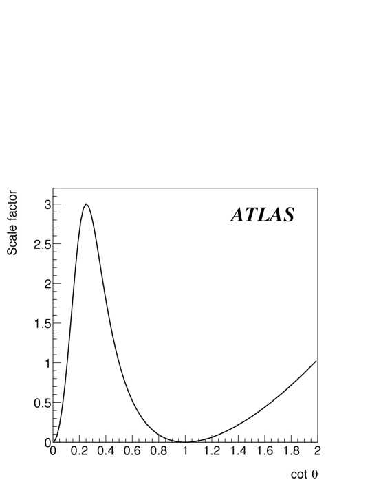
Figure 12: The $\cot\theta$ dependence of the production rate times branching ratio $Z_{H}\to Zh$.

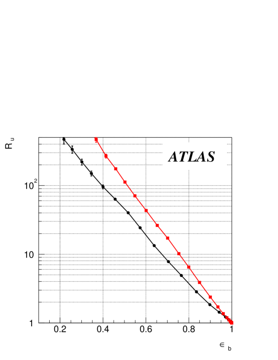
Figure 13: Plot showing the tagging efficiency for $b-$jets as a function of the rejection factor against light quark jets. The upper curve shows the result from the benchmark ATLAS sample of bottom quarks from a Higgs decay of mass 400 GeV produced in association with a $W$  [13]. The lower curve shows the result from the higher energy $b-$quarks from the $Z_{H}\to Zh$ sample.

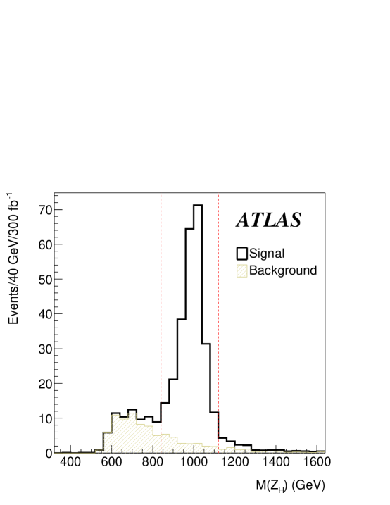
Figure 14: Invariant mass of the $Zh$ system reconstructed from the $\ell^{+}\ell^{-}b\overline{b}$ final state showing the signal from a $Z_{H}$ of mass 1000 GeV with $\cot\theta=0.5$ above the Standard Model background. The vertical lines define the signal region.

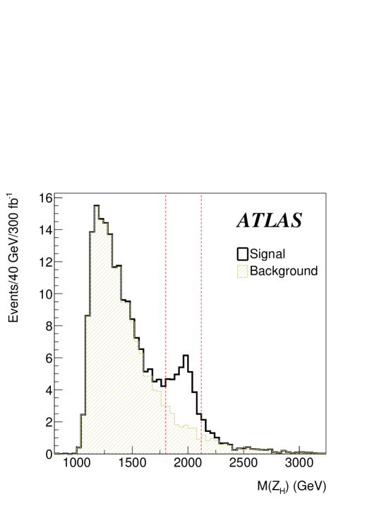
Figure 15: As in Figure 14 except that the $Z_{H}$ mass is 2 TeV.

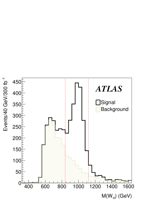
Figure 16: Invariant mass of the $Wh$ system reconstructed from the $\ell^{+}\nu b\overline{b}$ final state showing the signal from a $W_{H}$ of mass 1000 GeV with $\cot\theta=0.5$ above the Standard Model background. The vertical lines define the signal region.

The decay $h\to\gamma\gamma$ has a much smaller rate. Nevertheless it provides a very characteristic signal. A preliminary event selection requiring two isolated photons, one having $p_{T}>25$ GeV and the other $p_{T}>40$ GeV and both with $\left|\eta\right|<2.5$ was made. This requirement ensures that the events are triggered. The invariant mass of the two photon system is required to be within $2\sigma$ of the Higgs mass, $\sigma$ being the measured mass resolution of the diphoton system. The reconstructed jets in the event are then combined in pairs and the pair with invariant mass closest to $M_{W}$ was selected. If this pair has a combined $p_{T}>200$ GeV, its mass was corrected to the $W$ mass and then combined with the $\gamma\gamma$ system. The mass distribution of the resulting system is shown in Figure 17  [20]. The $W$ from the decay of $W_{H}$ is expected to have large $p_{T}$. Consequently it is possible for the jets from the $W$ have coalesced into a single jet. To allow for this possibility, if the jet pair has $p_{T}<200$ GeV it is not used. Rather, the $\gamma\gamma$ system is combined with any jet that has an invariant mass consistent with a $W$ and added to Figure 17. This figure shows a reconstructed mass peak at the common mass of $W_{H}$ and $Z_{H}$ of 1000 GeV; note that the states are expected to be almost degenerate in the model. 50% of the $\gamma\gamma+jet+jet$ signal events are accepted into the figure. The contribution from $W_{H}$ and $Z_{H}$ is shown separately, the former dominates due to its larger production rate. But, the mass resolution in the jet system is not good enough to resolve the $W$ from the $Z$ when both decay hadronically. We cannot, therefore, separate the signals from the $W_{H}$ and $Z_{H}$. The presence of the two photons with a mass comparable to the Higgs mass ensures that the background is small. The background arises from either direct Higgs production or the QCD production of di-photons, these are both shown on the figure. The requirements on the jet system and photon acceptance remove 98% of the Higgs background.

The signal to background ratio is large enough that a signal can also be seen without reconstructing the jet system. Since the $W_{H}$ and $Z_{H}$ are produced singly, with small transverse momentum, there is a “Jacobian” peak in the transverse momentum distribution of the Higgs. This momentum is reconstructed with great precision from its $\gamma\gamma$ decay mode owing to the excellent electromagnetic calorimetry of the ATLAS detector. Of course, this inclusive signal cannot distinguish $W_{H}$ from $Z_{H}$. The inclusive nature of this signal results in a small improvement in the efficiency as the jets from $W$ or $Z$ are not reconstructed. The sensitivity of this inclusive signature is approximately the same as that from reconstructing the hadronic decay of $W/Z$  [20].

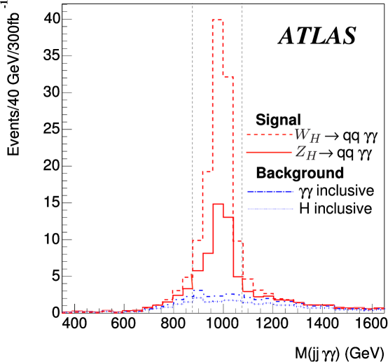
Figure 17: Plot showing the invariant mass of $\gamma\gamma+Jets$ system, where the $\gamma\gamma$ system has a mass consistent with the Higgs mass of 120 GeV and the $Jet$ system is selected as described in the text. The largest histogram arises from $W_{H}\to hW$ and the second largest from $Z_{H}\to hZ$ for $\cot\theta=0.5$ and a $Z_{H}$ and $W_{H}$ mass of 1000 GeV. The backgrounds from Higgs production (dotted) and the QCD production of di-photons (dashed) are also shown. The vertical lines define the signal region.

In the case of $A_{H}$ production and decay to $Zh$, the rates depend on the mixings and so we present the sensitivity in terms of a cross-section that allows reinterpretation of these results to other models. Using the method described above, we show in Figure 18 the value of the production cross-section times branching ratio needed to obtain discovery in the channels $A_{H}\to Zh\to\ell\ell b\overline{b}$ and $A_{H}\to Zh\to\hbox{jets }\gamma\gamma$.

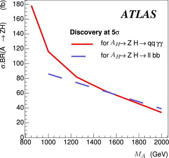
Figure 18: Plot showing the minimum value of the production cross-section times branching ratio needed to obtain discovery in the channels $A_{H}\to Zh\to\ell\ell b\overline{b}$ and $A_{H}\to Zh\to jets\gamma\gamma$ as a function of the $A_{H}$ mass.

4 Search for $\phi^{++}$

The doubly-charged Higgs boson could be produced in pairs and decay into leptonic final states via $q\overline{q}\to\phi^{++}\phi^{--}\to 4\ell$. While this would provide a very clean signature, it will not be considered here since the mass reach in this channel is poor due to the small cross-section. The coupling of $\phi^{++}$ to $W^{+}W^{+}$ allows it to be produced singly via $WW$ fusion processes of the type $dd\to uu\phi^{++}\to uuW^{+}W^{+}$. This can lead to events containing two leptons of the same charge, and missing energy from the decays of the $W$’s. The $\phi WW$ coupling is determined by $v^{\prime}$, the vacuum expectation value (vev) of the neutral member of the triplet. This cannot be too large as its presence causes a violation of custodial SU(2) which is constrained by measurements of the $W$ and $Z$ masses. We have examined the sensitivity of searches at the LHC in terms of $v^{\prime}$ and the mass of $\phi^{++}$. For $v^{\prime}=25$ MeV and a mass of 1000 TeV, the rate for production of $\phi^{++}$ followed by the decay to $WW$ is 4.9 fb if the $W$’s have $\left|\eta\right|<3$ and $p_{T}>200$ GeV.  [15]. The simulation discussed below is normalized to this rate. As in the case of Standard Model Higgs searches using the $WW$ fusion process  [13], the presence of jets at large rapidity must be used to suppress backgrounds. The event selection closely follows that used in searches for a heavy Standard Model Higgs via the $WW$ fusion process  [21] and is as follows.

• Two reconstructed positively charged isolated leptons (electrons or muons) with $\left|\eta\right|<2.5$.

• One of the leptons was required to have $p_{T}>150$ GeV and the other $p_{T}>20$ GeV.

• The leptons are not balanced in transverse momentum: $\left|p_{T1}-p_{T2}\right|>200$ GeV.

• The difference in pseudorapidity of the two leptons $\left|\eta_{1}-\eta_{2}\right|<2$.

• $\hbox to0.0pt{\hbox to7.95831pt{\hfil/\hfil}\hss}E_{T}>50$ GeV.

• Two jets each with $p_{T}>15$ GeV, with rapidities of opposite sign, separated in rapidity $\left|\eta_{1}-\eta_{2}\right|>5$; one jet has $E>200$ GeV and the other $E>100$ GeV.

The presence of the leptons ensures that the events are triggered. The invarient mass of the $WW$ system cannot be reconstructed. The signal can be observed using a mass variable made from the observed leptons (${\bf p_{1}}$ and ${\bf p_{2}}$) and the missing transverse energy as follows.

$$m^{2}_{T}=(E_{1}+E_{2}+\left|\hbox to0.0pt{\hbox to7.95831pt{\hfil/\hfil}\hss}E_{T}\right|)^{2}-({\bf p_{1}}+{\bf p_{2}}+{\bf\hbox to0.0pt{\hbox to7.95831pt{\hfil/\hfil}\hss}E_{T}})^{2}$$

The reconstructed mass distributions are shown in Figures 19 and 20 for masses of 1000 and 1500 GeV. Standard Model backgrounds are shown separately on the figures  [23]. In the region where $m^{2}_{T}>500$ GeV, the above kinematic cuts accept 50% of the $\phi^{++}\to\ell^{+}\nu\ell^{+}\nu$ events for $\phi^{++}$ of mass 1 TeV.

The dominant background is from non-resonant $qqW^{+}W^{+}$ production, including WW scattering as well as QED and QCD processes involving quark scattering where $W$’s are radiated from the quarks. The background from the non-resonant $WW$ scattering, which has the same topology as the signal, was generated using CompHep  [16]. In the region where $m^{2}_{T}>500$ GeV, the above kinematic cuts accept 5% of the $WW\to\ell^{+}\nu\ell^{+}\nu$ process; the leptons being less energetic that those from the signal. For a Higgs mass of 120 GeV, the contribution of longitudinal WW scattering is very small. No $t\overline{t}$ events survive the cuts; the forward jet tag being particularly effective in this case  [23]. The residual background from $WZ$ events is below 10% of that from $qqW^{+}W^{+}$. Note that the rates shown in these figures are small and the signal does not appear as a clear peak. The process is very demanding of luminosity, the ability to detect forward jets at relatively small $p_{T}$, and the ability to control backgrounds. These issues cannot be fully addressed until actual data is available. At this stage, we can only estimate our sensitivity using our current, best estimates, of the these issues. Since the cross-section for a $\phi^{++}$ of a fixed mass is proportional to $(v^{\prime})^{2}$, the simulation can be used to determine the sensitivity. Requiring at least 10 events for $M_{T}>700(1000)$ GeV for $m_{\phi}=1000(1500)$ GeV and a value of $S/\sqrt{B}>5$ implies that discovery is possible if $v^{\prime}>29(54)$ GeV. Such values are larger than the constraint of 15 MeV from electro-weak fits [15].

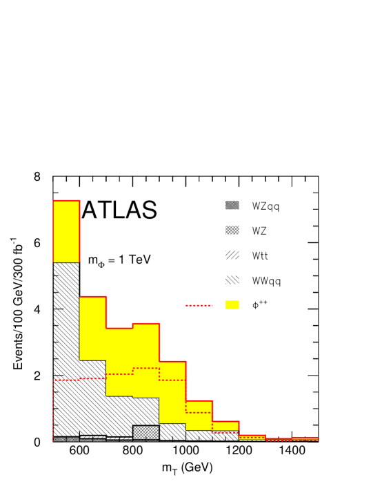
Figure 19: The mass distribution $M_{T}$, see text, for a $\phi^{++}$ of mass 1000 GeV and $v^{\prime}=25$ GeV. The dashed histogram shows the signal alone and the solid shows the sum of signal and backgrounds. The components of the background are also shown separately.

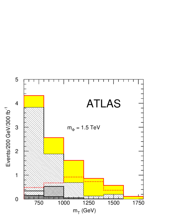
Figure 20: As in Figure 19 except that the mass is 1500 GeV. The legend is the same as on Figure 19.

In view of this rather poor sensitivity, it is worth considering other possible signals for the Higgs sector. The $\phi^{+}$ and $\phi^{0}$ can also be produced by gauge boson fusion leading to $WZ$ and $W^{+}W^{-}$ final states. The latter is similar qualitatively to the production of a heavy Standard Model Higgs boson with reduced couplings. The background in these channels is larger than that for $\phi^{++}$, so observation is likely to be more difficult. Doubly charged Higgs bosons also occur in some left-right symmetric models  [22]. In these models the boson can decay via a lepton flavor violating coupling to $\ell^{+}\ell^{+}$. In the Littlest Higgs model under consideration the decay $\phi^{++}\to\ell^{+}\ell^{+}$ does not occur so this search is not effective.

5 Model Constraints and Conclusions

We have demonstrated, using a series of examples, how measurements using the ATLAS detector at the LHC can be used to reveal the three characteristic particles of the Little Higgs models. The $T$ quark is observable up to masses of approximately 2.5 TeV via its decay to $Wb$. Sensitivity in $Zt$ or $Zh$ is lower but it still extends over the range expected in the model provided that the Higgs mass is not too large. The decays of $T$ to $Wb$ and $Zt$ are, of course, independent of the Higgs mass. In the case of $Zh$ the sensitivity will depend on the Higgs mass. The $h\to b\overline{b}$ channel continues to be effective until Higgs mass exceeds 150 GeV or so when it becomes too small to exploit due to the falling branching ratio for this decay. The studies presented in section 2.3 are valid up to this mass. In this case ATLAS will be able to detect $T$ in its three decay channels and provide a definitive test of the model. For larger Higgs masses, the channels with excellent signal to background ratios such as $h\to\ell^{+}\ell^{-}\ell^{+}\ell^{-}$ and $h\to\ell^{+}\ell^{-}\nu\nu$, have small effective branching ratios which will severely restrict a search using them. However, ATLAS will still be able to detect the $Wb$ and $Zt$ final states which will enable us to distinguish $T$ from a 4^th generation quark.

In the case of the new gauge bosons, the situation is summarized in Figures 21 and 22. The former shows the accessible regions via the $e^{+}e^{-}$ final states of $Z_{H}$ and $A_{H}$ as a function of the mixing angles and the scale $f$ that determines the masses. Except for a small region near $\tan\theta^{\prime}=1.3$ and $f>7.5$ TeV, we are sensitive to the whole range expected in the model. However observation of such a gauge boson will not prove that it is of the type predicted in the Little Higgs Models. In order to do this, the decays to the Standard Model bosons must be observed. Figure 22 shows the sensitive regions for decays of $Z_{H}$ and $W_{H}$ into various final states as a function of $\cot\theta$ and the masses. It can be seen that several decay modes are only observable for smaller masses over a restricted range of $\cot\theta$ where the characteristic decays $Z_{H}\to Zh$ and $W_{H}\to Wh$ can be seen. There is a small region at very small values of $\cot\theta$ where the leptonic decays are too small, and only the decays to $W/Z$ can be seen. One of the channels shown on this plot, the decay to $h$, is sensitive to the Higgs mass. The channel used for this analysis, $h\to\gamma\gamma$ becomes less effective as the Higgs mass increases. At the assumed mass of 120 GeV, the branching ratio is approximately 2%. As the rates shown in Figure 17 scale with this branching ratio, we expect that this mode is not visible for Higgs masses above 150 GeV. Other decays of the Higgs have not yet been investigated. To summarize, the new gauge bosons are observable over the entire mass range predicted. Measurements of more than one final state are possible in certain regions of parameter space.

In the case of $\phi^{++}$ the situation is not so promising. The Higgs sector is the least constrained by fine tuning arguments and this particle’s mass can extend up to 10 TeV. We are only sensitive to masses up to 2 TeV or so provided that $v^{\prime}$ is large enough. Other “Little Higgs” models  [10] have a different Higgs structure that is similar to models with more than one Higgs doublet that have been studied in the past. Work is needed to evaluate the sensitivity of the LHC to these models.

In conclusion, we have investigated the signatures of the Littlest Higgs model using ATLAS at the LHC. We have seen that the LHC, with its full luminosity, is fully sensitive to the new quarks and gauge bosons. The new Higgs particles may be out of reach.

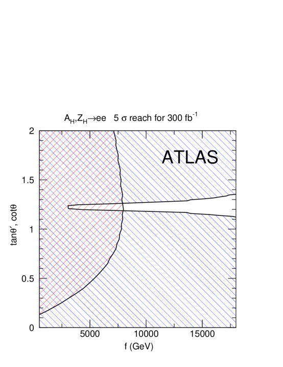
Figure 21: Plot showing the accessible regions for $5\sigma$ discovery of the neutral gauge bosons $A_{H}$ and $Z_{H}$ as a function of the scale $f$ where the additional symmetry is broken. The variable $\cot\theta$ applies to the $Z_{H}$ for which the red region (lines running from bottom-left to top-right) is accessible. The blue region (lines running from top-left to bottom-right) shows the $A_{H}$ accessible region as a function of $\tan\theta^{\prime}$.

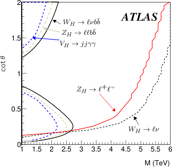
Figure 22: Plot showing the accessible regions for $5\sigma$ discovery of the gauge bosons $W_{H}$ and $Z_{H}$ as a function of the mass and $\cot\theta$ for the various final states. The regions to the left of the lines are accessible with 300 ${\rm fb}^{-1}$.

References

- [1] N. Arkani-Hamed, A. G. Cohen and H. Georgi, JHEP 0207, 020 (2002).
- [2] N. Arkani-Hamed, A. G. Cohen and H. Georgi, Phys. Lett. B 513, 232 (2001).
- [3] H. Georgi and A. Pais, Phys. Rev. D 10, 539 (1974).
- [4] D. B. Kaplan, H. Georgi and S. Dimopoulos, Phys. Lett. B 136, 187 (1984).
- [5] N. Arkani-Hamed, A. G. Cohen, E. Katz and A. E. Nelson, JHEP 0207, 034 (2002).
- [6] N. Arkani-Hamed, A. G. Cohen, E. Katz, A. E. Nelson, T. Gregoire and J. G. Wacker, JHEP 0208, 021 (2002). [arXiv:hep-ph/0206020].
- [7] C. Csaki, J. Hubisz, G. D. Kribs, P. Meade and J. Terning, arXiv:hep-ph/0211124.
- [8] J. L. Hewett, F. J. Petriello and T. G. Rizzo, arXiv:hep-ph/0211218.
- [9] S. Chang, arXiv:hep-ph/0306034.
- [10] D. E. Kaplan and M. Schmaltz, arXiv:hep-ph/0302049.
- [11] T. Sjostrand, L. Lonnblad and S. Mrenna, arXiv:hep-ph/0108264.
- [12] http://www.hep.ucl.ac.uk/atlas/atlfast/UserGuide.html
- [13] ATLAS Collaboration, “ATLAS Physics and Detector Performance Technical Design Report,” LHCC 99-14/15. Chapter 10.
- [14] A. Artamonov et al., ATL-SOFT-95-014; GEANT-3, CERN program library W5013 Geneva, 1994.
- [15] T. Han, H. E. Logan, B. McElrath and L. T. Wang, arXiv:hep-ph/0301040.
- [16] A. Pukhov et al., arXiv:hep-ph/9908288.
- [17] D. Costanzo, ATL-COM-PHYS-2003-036. “Reference to be updated”.
- [18] B. P. Kersevan and E. Richter-Was, arXiv:hep-ph/0201302.
- [19] G. Burdman, M. Perelstein and A. Pierce, arXiv:hep-ph/0212228.
- [20] J. E. Garcia, M. Lechowski, E. Ros, and D. Rousseau, ATL-PHYS-2004-001.
- [21] S. Asai et al., SN-ATLAS-2003-024.
- [22] K. Huitu, J. Maalampi, A. Pietila and M. Raidal, Nucl. Phys. B 487 (1997) 27.
- [23] G. Azuelos, K. Benslama, and G. Coutoure, ATL-PHYS-2004-002.