Supersymmetric virtual effects in heavy quark pair production at LHC

Abstract

We consider the production of heavy ($b,t$) quark pairs at proton colliders in the theoretical framework of the MSSM. Under the assumption of a ”moderately” light SUSY scenario, we first compute the leading logarithmic MSSM contributions at one loop for the elementary processes of production from a quark and from a gluon pair in the 1 TeV c.m. energy region. We show that in the initial gluon pair case (dominant in the chosen situation at LHC energies) the electroweak and the strong SUSY contributions concur to produce an enhanced effect whose relative value in the cross sections could reach the twenty percent size for large $\tan\beta$ values in the realistic proton-proton LHC process.

I Introduction

One of the main goals of the future experiments at hadron colliders will be undoubtedly the search for supersymmetric particles. In the specific theoretical framework of the MSSM, a vast amount of literature already exists showing the expected experimental reaches for the different supersymmetric spectroscopies and parameters, both for the TEVATRON[1] and for the LHC[2] cases. For what concerns the possibility of direct production, nothing has to be added (in our opinion) to the existing studies, leading to the conclusion that, if any supersymmetric particle exists with a not unfairly large mass, it will not escape direct detection and identification.

A nice and special feature of the present and future hadron colliders is the fact that, on top of direct SUSY production, a complementary precision test of the involved model (assuming a preliminary discovery) is also in principle possible. This implies the study of virtual SUSY effects in the production of suitable (not necessarily supersymmetric) final states, in full analogy with the previous memorable analyses performed to test the Standard Model at LEP1, SLC and LEP2 [3]. For what concerns the realistic experimental accuracy requested by a similar search, one expects [4], [5] a possible relative few percent level. In this spirit, the existence of virtual SUSY effects as large as a relative ten percent or more should be carefully examined and investigated.

The aim of this preliminary paper is actually that of showing that the production of a final heavy ($b,t$) quark pair at LHC could be particularly convenient for the search of virtual SUSY effects. This is due to a number of technical features (cancellations of disturbing contributions at high energies, not negligible final quark masses,…) that will be thoroughly illustrated in the following Sections. In this preliminary analysis, we studied the electroweak and the SUSY QCD contributions to the subprocess initiated by $q\bar{q}$ and $gg$ partons and we limited our application to the invariant mass distribution of $PP\to q\bar{q}+...$ at LHC using standard quark and gluon structure functions. The rewarding result was that of finding that the SUSY electroweak and the SUSY QCD terms concur to produce an overall effect that can be as large as a relative twenty percent in the assumed light SUSY scenario. This effect is more due to the electroweak component than to the QCD component, essentially owing to the final heavy quark Yukawa contribution (proportional to the quark squared mass). The picture at one loop is in fact, surprisingly to us, practically the same that one would find in the case of electron-positron annihilation at LC [6], as we shall briefly discuss in this paper for sake of comparison. At the possible few percent experimental accuracy level [5], this effect should not escape a dedicated measurement, and could provide an important test of the (assumedly -and hopefully- discovered) supersymmetric scenario.

Technically speaking, this paper is organized as follows: Section 2 will be devoted to a description of the one-loop analysis for an initial $q\bar{q}$ state; in Section 3, the same description will be given for an initial $gg$ state and a brief comment will be given on the analogy of the results with those obtained for an initial electron-positron state; in Section 4, a numerical analysis of the possibly visible effects on the realistic proton-proton initiated process will be shown and a few conclusions will finally appear in Section 5.

II Initial $q\bar{q}$ state

We begin our analysis at the partonic level considering as initial states the light quark components of the proton (including the bottom component but ignoring the top quark one). At lowest $\alpha_{s}$ order the scattering amplitude is given by the Born terms schematically represented in Fig.1. The $s$-channel diagram of Fig.1a applies to all initial $q\bar{q}$ pair annihilation and leads to:

$$A^{\rm Born}_{s}=\sum_{i,j}a^{\rm Born~{}s}_{ij}[\bar{v}(\bar{q}){\lambda_{l}\gamma^{\mu}\over 2}P_{i}u(q)][\bar{u}(q^{\prime}){\lambda_{l}\gamma_{\mu}\over 2}P_{j}v(\bar{q}^{\prime})]$$ (1)

whereas the $t$-channel diagram will only apply to $b\bar{b}\to b\bar{b}$ scattering (because we shall neglect the $t\bar{t}\to t\bar{t}$ contribution) and writes:

$$A^{\rm Born}_{t}=\sum_{i,j}a^{\rm Born~{}t}_{ij}[\bar{v}(\bar{q}){\lambda_{l}\gamma^{\mu}\over 2}P_{i}v(\bar{q})][\bar{u}(q){\lambda_{l}\gamma_{\mu}\over 2}P_{j}u(q)]$$ (2)

where $i,j$ refer to $R$ or $L$ quark chiralities with $P_{R,L}={1\pm\gamma^{5}\over 2}$; $l$ is the intermediate gluon colour state and

$$a^{\rm Born~{}s}_{ij}={4\pi\alpha_{s}\over s}~{}~{}~{}~{}~{}~{}~{}~{}~{}~{}~{}~{}~{}~{}~{}a^{\rm Born~{}t}_{ij}={4\pi\alpha_{s}\over t}$$ (3)

At the Born level, electroweak contributions only consist in the Drell-Yan process $q\bar{q}\to\gamma,Z\to q^{\prime}\bar{q}^{\prime}$ but the effect in the cross section will be reduced by a factor $\alpha^{2}/\alpha^{2}_{s}\simeq 0.01$ as compared to the QCD one and will be neglected at the expected LHC accuracy.

Our starting assumption, as already stated in the Introduction, will be the discovery of (at least some) supersymmetric particles. In this spirit, we shall examine the possibility of performing a precision test of the candidate model by looking at its higher order virtual effects in the considered heavy quark production at hadron colliders, starting from the determination of these effects at the partonic level. As a first case to be examined, we shall restrict our study to the MSSM framework. For what concerns the higher order diagrams to be retained, we must at this point make our strategy completely clear. In general, the higher order corrections to the considered processes will be of electroweak and of strong nature. We shall begin our analysis with the detailed study of the electroweak components given in the following Section IIa.

A Electroweak corrections

To the first order one-loop level the electroweak corrections will typically correspond to the diagrams schematically represented in Fig.2. Note that we considered in the electroweak sector both the SM components and the genuinely supersymmetric ones, that will be often denoted for simplicity with a (SUSY) apex. In our analysis, we shall not consider higher order (e.g. two loops) electroweak corrections. This (pragmatic) attitude is, at least, supported by the fact (that we showed in a previous paper[7]) that such terms at lepton colliders (LC) are only requested if the available c.m. energy of the process is beyond, roughly, the 1 TeV range. In our investigation of proton colliders, the structure of the leading electroweak corrections is essentially similar to the LC one (with straightforward modifications of the initial vertex contributions). To reproduce the benefit of the absence of hard resummation computations, we shall therefore be limited to c.m. energy values not beyond the 1 TeV limit.

Having fixed the considered energy range, a numerical evaluation at one loop can now be performed in a (reasonably) straightforward way. A great simplification can nonetheless be achieved under the assumption that the c.m. energy is sufficiently larger than all the masses of the (real and virtual) particles involved in the process. In this case, a logarithmic expansion of the so-called Sudakov kind can be adopted. All the details of such an approach for the specific MSSM model have been already exhaustively discussed in previous references for an initial electron-positron state[8],[9], but the results are essentially identical if the initial state is a $q\bar{q}$ pair (as we said, one must only modify in a straightforward way the initial vertex contribution). To avoid loss of space and time, we defer thus the reader to[8],[9] for details. The only relevant point that we want to make is the fact that the ”canonical” logarithmic expansion is given to next-to leading order, i.e. retaining the double and the linear logarithmic terms, and ignoring possible extra (e.g. constant) contributions. To this level, the remarkable simplification for the considered heavy quark final state is that only two SUSY parameters appear in the expansion. One parameter is $\tan\beta$, contained in the coefficient of the linear $ln$ of Yukawa origin; the second one is a (common) SUSY mass scale $M$, to be understood as an ”average” supersymmetric mass involved in the process.

Given the fact that the supersymmetric masses might be not particularly small (the existing limits for squark and gluino masses are at the moment consistent with a lower bound of approximately $300$ GeV[1],[10]) and taking into account the qualitative 1 TeV upper bound on the c.m. energy requested for the validity of a one-loop expansion, we shall adopt in this preliminary analysis a reasonable working compromise. In other words, we shall consider energy values in the 1 TeV range, and a SUSY scenario ”reasonably” light i.e. one in which all the relevant SUSY masses of the process are smaller than, approximately, $350-400$ GeV. This will encourage us to trust a conventional Sudakov expansion, supported by previous detailed numerical analyses given for electron-positron accelerators[11].

The previous discussion was related to the SUSY electroweak effects. Our attitude will be in conclusion that of considering both the SM and the SUSY components at the same one loop level. Strictly speaking, since we are only interested in the SUSY effect, we could even ignore the SM contribution. The reason why we retain it is simply that it is easy to estimate it and interesting to show the ”SUSY enhancement” in the MSSM overall correction.

After this long but, we hope, sufficiently clear discussion, we are now ready to illustrate the one-loop numerical details. With this aim, we shall start from the electroweak diagrams of Fig.2 and write, following our previous notations [7, 8, 9]:

Electroweak logarithmic corrections on the amplitudes

For each $q\bar{q}\to q^{\prime}\bar{q}^{\prime}$ amplitude we can write, following ref.[9]:

$$A^{\rm 1~{}loop~{}ew}=A^{Born}[1+c^{\rm ew}]$$ (4)

with

$$c^{\rm ew}\equiv c_{in,~{}gauge}+c_{in,~{}Yuk}+c_{fin~{}gauge}+c_{fin,~{}Yuk}+c_{ang}$$ (5)

where $c_{in}$ refers to the universal (i.e. process independent) corrections due to the initial $q\bar{q}$ pair, $c_{fin}$ to the universal corrections due to the final $b\bar{b}$ or $t\bar{t}$ pair and $c_{ang}$ is a process and angular dependent correction typical of each $q\bar{q}\to q^{\prime}\bar{q}^{\prime}$ case. The Yukawa contributions are sizable only for $q$ (or $q^{\prime}$) being $b$ or $t$ quarks. The coefficients $c^{\rm ew}$ receive SM and SUSY contributions, depending on the quark chirality. The SM contributions are ($u$ represents both up and charmed quarks, and $d$ both down and strange quarks):

$$c^{u\bar{u}~{}SM}_{in,~{}gauge~{}L}=c^{t\bar{t}~{}SM}_{fin,~{}gauge~{}L}={\alpha(1+26c^{2}_{W})\over 144\pi s^{2}_{W}c^{2}_{W}}[3ln{s\over M^{2}_{W}}-ln^{2}{s\over M^{2}_{W}}]$$ (6)

$$c^{u\bar{u}~{}SM}_{in,~{}gauge~{}R}=c^{t\bar{t}~{}SM}_{fin,~{}gauge~{}R}={\alpha\over 9\pi c^{2}_{W}}[3ln{s\over M^{2}_{W}}-ln^{2}{s\over M^{2}_{W}}]$$ (7)

$$c^{d\bar{d}~{}SM}_{in,~{}gauge~{}L}=c^{b\bar{b}~{}SM}_{fin,~{}gauge~{}L}={\alpha(1+26c^{2}_{W})\over 144\pi s^{2}_{W}c^{2}_{W}}[3ln{s\over M^{2}_{W}}-ln^{2}{s\over M^{2}_{W}}]$$ (8)

$$c^{d\bar{d}~{}SM}_{in,~{}gauge~{}R}=c^{b\bar{b}~{}SM}_{fin,~{}gauge~{}R}={\alpha\over 36\pi c^{2}_{W}}[3ln{s\over M^{2}_{W}}-ln^{2}{s\over M^{2}_{W}}]$$ (9)

$$c^{b\bar{b}~{}SM}_{in,fin,~{}Yuk~{}L}=c^{t\bar{t}~{}SM}_{in,fin,~{}Yuk~{}L}=-~{}{\alpha\over 16\pi s^{2}_{W}}[{m^{2}_{t}\over M^{2}_{W}}+{m^{2}_{b}\over M^{2}_{W}}][ln{s\over M^{2}_{W}}]$$ (10)

$$c^{b\bar{b}~{}SM}_{in,fin,~{}Yuk~{}R}=-~{}{\alpha\over 8\pi s^{2}_{W}}[{m^{2}_{b}\over M^{2}_{W}}][ln{s\over M^{2}_{W}}]$$ (11)

$$c^{t\bar{t}~{}SM}_{in,fin,~{}Yuk~{}R}=-~{}{\alpha\over 8\pi s^{2}_{W}}[{m^{2}_{t}\over M^{2}_{W}}][ln{s\over M^{2}_{W}}]$$ (12)

$$c^{q\bar{q}~{}q^{\prime}\bar{q}^{\prime}~{}SM}_{ang~{}ij}=-~{}{\alpha\over 4\pi}[ln{1-cos\theta\over 1+cos\theta}][8Q_{q}Q_{q^{\prime}}+2{g^{Z}_{qi}g^{Z}_{fj}\over s^{2}_{W}c^{2}_{W}}][ln{s\over M^{2}_{W}}]$$ (13)

This last angular dependent term refers to chirality states $(ij)=(LL,LR,RL,RR)$ and involves the quark charges $Q_{q}$ and the $Zq\bar{q}$ couplings $g^{Z}_{qL}=I^{3}_{qL}(2-4|Q_{q}|s^{2}_{W})$, $g^{Z}_{qR}=-2Q_{q}s^{2}_{W}$.

The additional SUSY contributions affect only the universal parts:

$$c^{u\bar{u}~{}SUSY}_{in,~{}gauge~{}L}=c^{t\bar{t}~{}SUSY}_{fin,~{}gauge~{}L}=-~{}{\alpha(1+26c^{2}_{W})\over 144\pi s^{2}_{W}c^{2}_{W}}[ln{s\over M^{2}}]$$ (14)

$$c^{u\bar{u}~{}SUSY}_{in,~{}gauge~{}R}=c^{t\bar{t}~{}SUSY}_{fin,~{}gauge~{}R}=-~{}{\alpha\over 9\pi c^{2}_{W}}[ln{s\over M^{2}}]$$ (15)

$$c^{d\bar{d}~{}SUSY}_{in,~{}gauge~{}L}=c^{b\bar{b}~{}SUSY}_{fin,~{}gauge~{}L}=-~{}{\alpha(1+26c^{2}_{W})\over 144\pi s^{2}_{W}c^{2}_{W}}[ln{s\over M^{2}}]$$ (16)

$$c^{d\bar{d}~{}SUSY}_{in,~{}gauge~{}R}=c^{b\bar{b}~{}SUSY}_{fin,~{}gauge~{}R}=-~{}{\alpha\over 36\pi c^{2}_{W}}[ln{s\over M^{2}}]$$ (17)

$$c^{b\bar{b}~{}SUSY}_{in,fin,~{}Yuk~{}L}=c^{t\bar{t}~{}SUSY}_{in,fin,~{}Yuk~{}L}=-~{}{\alpha\over 16\pi s^{2}_{W}}[{m^{2}_{t}\over M^{2}_{W}}(1+2\cot^{2}\beta)+{m^{2}_{b}\over M^{2}_{W}}(1+2\tan^{2}\beta)][ln{s\over M^{2}}]$$ (18)

$$c^{b\bar{b}~{}SUSY}_{in,fin,~{}Yuk~{}R}=-~{}{\alpha\over 8\pi s^{2}_{W}}[{m^{2}_{b}\over M^{2}_{W}}(1+2\tan^{2}\beta)][ln{s\over M^{2}}]$$ (19)

$$c^{t\bar{t}~{}SUSY}_{in,fin,~{}Yuk~{}R}=-~{}{\alpha\over 8\pi s^{2}_{W}}[{m^{2}_{t}\over M^{2}_{W}}(1+2\cot^{2}\beta)][ln{s\over M^{2}}]$$ (20)

One can see (as emphasized in ref.[9]) that the total MSSM gauge correction is quite simply obtained by replacing the logarithmic SM factor $[3ln{s\over M^{2}_{W}}-ln^{2}{s\over M^{2}_{W}}]$ by $[2ln{s\over M^{2}_{W}}-ln^{2}{s\over M^{2}_{W}}]$ and the total MSSM Yukawa correction by replacing the SM $m^{2}_{t}$ by $2m^{2}_{t}(1+\cot^{2}\beta)$ and $m^{2}_{b}$ by $2m^{2}_{b}(1+\tan^{2}\beta)$.

Results for angular distributions, averaged over initial, summed over final polarizations

We now list explicitely the complete MSSM results for each subprocess. According to the rules given just above it is easy to separate the pure SM and the additional SUSY parts. We first consider the subprocesses involving only the annihilation channel of Fig.1a and Fig.2, and write:

$${d\sigma^{1~{}loop}\over dcos\theta}={d\sigma^{Born}\over dcos\theta}+{\pi\alpha^{2}_{s}\over 18s}\{~{}(1+\cos^{2}\theta)~{}[S]+2\cos\theta~{}[D]~{}\}$$ (21)

with

$${d\sigma^{Born}(q\bar{q}\to q^{\prime}\bar{q}^{\prime})\over dcos\theta}={\pi\alpha^{2}_{s}\over 9s}(1+\cos^{2}\theta)$$ (22)

and

For $u\bar{u}\to b\bar{b}$

$$S_{u\bar{u}b\bar{b}} = {\alpha\over 72\pi s^{2}_{W}c^{2}_{W}}(54-32s^{2}_{W})[2ln{s\over M^{2}_{W}}-ln^{2}{s\over M^{2}_{W}}]$$ (25)

$$-{\alpha\over 4\pi s^{2}_{W}}[{m^{2}_{t}\over M^{2}_{W}}(1+\cot^{2}\beta)+{3m^{2}_{b}\over M^{2}_{W}}(1+\tan^{2}\beta)][ln{s\over M^{2}_{W}}]$$

$$-~{}{\alpha(4s^{2}_{W}-9)\over 18\pi s^{2}_{W}c^{2}_{W}}ln{1-\cos\theta\over 1+\cos\theta}[ln{s\over M^{2}_{W}}]$$

$$D_{u\bar{u}b\bar{b}} = {\alpha\over 2\pi s^{2}_{W}c^{2}_{W}}ln{1-\cos\theta\over 1+\cos\theta}[ln{s\over M^{2}_{W}}]$$ (26)

For $d\bar{d}\to b\bar{b}$

$$S_{d\bar{d}b\bar{b}} = {\alpha\over 72\pi s^{2}_{W}c^{2}_{W}}(54-44s^{2}_{W})[2ln{s\over M^{2}_{W}}-ln^{2}{s\over M^{2}_{W}}]$$ (29)

$$-~{}{\alpha\over 4\pi s^{2}_{W}}[{m^{2}_{t}\over M^{2}_{W}}(1+\cot^{2}\beta)+{3m^{2}_{b}\over M^{2}_{W}}(1+\tan^{2}\beta)][ln{s\over M^{2}_{W}}]$$

$$+{\alpha(8s^{2}_{W}-9)\over 18\pi s^{2}_{W}c^{2}_{W}}ln{1-\cos\theta\over 1+\cos\theta}[ln{s\over M^{2}_{W}}]$$

$$D_{d\bar{d}b\bar{b}} = -~{}{\alpha\over 2\pi s^{2}_{W}c^{2}_{W}}ln{1-\cos\theta\over 1+\cos\theta}[ln{s\over M^{2}_{W}}]$$ (30)

For $u\bar{u}\to t\bar{t}$

$$S_{u\bar{u}t\bar{t}} = {\alpha\over 36\pi s^{2}_{W}c^{2}_{W}}(27-10s^{2}_{W})[2ln{s\over M^{2}_{W}}-ln^{2}{s\over M^{2}_{W}}]$$ (33)

$$-{\alpha\over 4\pi s^{2}_{W}}[{3m^{2}_{t}\over M^{2}_{W}}(1+\cot^{2}\beta)+{m^{2}_{b}\over M^{2}_{W}}(1+\tan^{2}\beta)][ln{s\over M^{2}_{W}}]$$

$$-~{}{\alpha(16s^{2}_{W}+9)\over 18\pi s^{2}_{W}c^{2}_{W}}ln{1-\cos\theta\over 1+\cos\theta}[ln{s\over M^{2}_{W}}]$$

$$D_{u\bar{u}t\bar{t}} = -~{}{\alpha\over 2\pi s^{2}_{W}c^{2}_{W}}ln{1-\cos\theta\over 1+\cos\theta}[ln{s\over M^{2}_{W}}]$$ (34)

For $d\bar{d}\to t\bar{t}$

$$S_{d\bar{d}t\bar{t}} = {\alpha\over 36\pi s^{2}_{W}c^{2}_{W}}(27-16s^{2}_{W})[2ln{s\over M^{2}_{W}}-ln^{2}{s\over M^{2}_{W}}]$$ (37)

$$-~{}{\alpha\over 4\pi s^{2}_{W}}[{3m^{2}_{t}\over M^{2}_{W}}(1+\cot^{2}\beta)+{m^{2}_{b}\over M^{2}_{W}}(1+\tan^{2}\beta)][ln{s\over M^{2}_{W}}]$$

$$-{\alpha(4s^{2}_{W}-9)\over 18\pi s^{2}_{W}c^{2}_{W}}ln{1-\cos\theta\over 1+\cos\theta}[ln{s\over M^{2}_{W}}]$$

$$D_{d\bar{d}t\bar{t}} = ~{}{\alpha\over 2\pi s^{2}_{W}c^{2}_{W}}ln{1-\cos\theta\over 1+\cos\theta}[ln{s\over M^{2}_{W}}]$$ (38)

For $b\bar{b}\to t\bar{t}$

$$S_{b\bar{b}t\bar{t}} = {\alpha\over 36\pi s^{2}_{W}c^{2}_{W}}(27-16s^{2}_{W})[2ln{s\over M^{2}_{W}}-ln^{2}{s\over M^{2}_{W}}]$$ (41)

$$-~{}{\alpha\over 4\pi s^{2}_{W}}[{4m^{2}_{t}\over M^{2}_{W}}(1+\cot^{2}\beta)+{4m^{2}_{b}\over M^{2}_{W}}(1+\tan^{2}\beta)][ln{s\over M^{2}_{W}}]$$

$$-{\alpha(4s^{2}_{W}-9)\over 18\pi s^{2}_{W}c^{2}_{W}}ln{1-\cos\theta\over 1+\cos\theta}[ln{s\over M^{2}_{W}}]$$

$$D_{b\bar{b}t\bar{t}} = ~{}{\alpha\over 2\pi s^{2}_{W}c^{2}_{W}}ln{1-\cos\theta\over 1+\cos\theta}[ln{s\over M^{2}_{W}}]$$ (42)

In the special case of $b\bar{b}\to b\bar{b}$ we have to add the annihilation amplitude of Fig.1a and of Fig.2, and the scattering amplitude of Fig.1b and of the $s\to t$ crossed diagrams of Fig.2. This leads to the result

$${d\sigma^{1~{}loop}(b\bar{b}\to b\bar{b})\over dcos\theta} = {d\sigma^{Born}(b\bar{b}\to b\bar{b})\over dcos\theta}\{~{}1+{\alpha\over 72\pi s^{2}_{W}c^{2}_{W}}(27-22s^{2}_{W})[2ln{s\over M^{2}_{W}}-ln^{2}{s\over M^{2}_{W}}]$$ (47)

$$-~{}{\alpha\over 4\pi s^{2}_{W}}[{m^{2}_{t}\over M^{2}_{W}}(1+\cot^{2}\beta)+{3m^{2}_{b}\over M^{2}_{W}}(1+\tan^{2}\beta)][ln{s\over M^{2}_{W}}]~{}\}$$

$$-~{}{\alpha^{2}_{s}\alpha\over 18s}[ln{s\over M^{2}_{W}}]~{}\{~{}({18-8s^{2}_{W}\over 9s^{2}_{W}c^{2}_{W}})(~{}[{u^{2}\over s^{2}}-~{}{u^{2}\over 3st}]ln{1-\cos\theta\over 1+\cos\theta}$$

$$-[{u^{2}\over t^{2}}-~{}{u^{2}\over 3st}]ln{1+\cos\theta\over 2})~{}+{27-22s^{2}_{W}\over 9s^{2}_{W}c^{2}_{W}}[{u^{2}+s^{2}\over t^{2}}-~{}{u^{2}\over 3st}]ln{1-\cos\theta\over 2}$$

$$-~{}({4s^{2}_{W}\over 9s^{2}_{W}c^{2}_{W}})(~{}{2t^{2}\over s^{2}}ln{1-\cos\theta\over 1+\cos\theta}-~{}{2s^{2}\over t^{2}}~{}ln{1+\cos\theta\over 2}~{})~{}\}$$

with

$${d\sigma^{Born}(b\bar{b}\to b\bar{b})\over dcos\theta}={2\pi\alpha^{2}_{s}\over 9s}~{}[{u^{2}+t^{2}\over s^{2}}+{u^{2}+s^{2}\over t^{2}}-{2u^{2}\over 3st}]$$ (48)

In the expression (47), the first part (which factorizes the Born term) is the universal effect including the gauge term and the double Yukawa effect, whereas the second part is the angular dependent effect from s and from t channels (one can check, restricting to the $1/s^{2}$ terms, that one recovers the previous $d\bar{d}\to b\bar{b}$ case); the $s\to t$ crossing relation between annihilation and scattering contributions is also clearly satisfied.

Having completed the discussion of the electroweak SUSY effect, we now move in the following subsection IIb to the discussion of the strong (QCD) SUSY correction.

B QCD SUSY correction

A preliminary statement to be made before entering the discussion of the QCD SUSY corrections is that we shall treat this effect under the same assumptions that we adopted for the electroweak sector, subsection IIa. In other words, we shall still concentrate our analysis on c.m. energy values in the 1 TeV region, assuming the previously considered ”reasonably” light SUSY scenario. This will allow us to use the same kind of simple logarithmic expansion that was exploited in the electroweak case, at the one loop level.

For what concerns the expected validity of a one-loop perturbative expansion, the situation is now, though, drastically different from that of subsection IIa, and requires a precise subtle choice of strategy. It is actually well-known[12] that, in the SM domain, the one-loop QCD correction is not accurate enough and higher order terms seem to be fundamental. This is understandable in an extremely simplified fashion as a consequence of the small scale which enters the SM running of $\alpha_{s}$. In this qualitative picture, one would expect that the corresponding SUSY effects do not share this dramatic problem, owing to the much larger mass scale involved. This would justify the expectation that, for the restricted subset of SUSY QCD corrections, a one-loop calculation can be sufficient.

Another essential difference between the SM QCD and the SUSY QCD corrections is that in the SM part the infrared logarithms arising from virtual gluon contributions cancel against those occurring in soft real gluon emission, leaving only ”constant” terms. In the SUSY case, large logarithms of virtual origin and scaled by the average SUSY mass will remain. A practical attitude seems to be therefore that of isolating the SM higher order QCD effects, considering them as a ”known” quantity, much in analogy with what is done for the canonical QED corrections, and to factorize an explicit one-loop term containing the genuine SUSY QCD correction, to be added in the usual one-loop philosophy to the electroweak one. This is the approach that we shall follow in the rest of the paper, which is, as we said, only interested in the evaluation of the genuine overall SUSY effect.

Having made this preliminary statement, we move now to the evaluation of the QCD SUSY effects at one loop. These are represented schematically in Fig.3, and can be classified in two quite different sectors, respectively of vertex kind and of RG origin. The first ones are essentially similar to analogous electroweak vertices of Sudakov kind, with a simple replacement of gauginos by gluinos. They produce, in the adopted ”Sudakov regime”, the following effect on the amplitude for each external $q\bar{q}$ pair

$$c^{q\bar{q}~{}SUSY~{}QCD}_{L,R}=-~{}{\alpha_{s}\over 3\pi}ln{s\over M^{2}}$$ (49)

which leads to an additional coefficient in the series eq.(4,5) equal to twice this value for a $q\bar{q}\to q^{\prime}\bar{q}^{\prime}$ annihilation amplitude or for a $q\bar{q}\to q\bar{q}$ scattering amplitude, i.e. eq.(4) is replaced by

$$A^{Born}[1+c^{\rm ew}-~{}{2\alpha_{s}\over 3\pi}ln{s\over M^{2}}]$$ (50)

From eq.(50) a rather important (in our opinion) feature can be stressed. Numerically, one sees that for ”reasonable” values of the squark and gluino masses, the QCD SUSY vertex effect has a numerical value of approximately 5 percent at 1 TeV c.m. energy. This supports our assumption that higher order terms can be neglected, as we shall do in this paper. Note also that the size of the effect is smaller than that of the analogous electroweak component, particularly for large $\tan\beta$ values in the Yukawa couplings. In other words, at the one loop level, electroweak SUSY corrections appear to be ”stronger” than the corresponding QCD ones, in full analogy with a similar feature first stressed in the electron-positron case[13].

From a practical point of view, the very welcome feature that characterizes the QCD SUSY vertex is the fact that the sign of the one-loop effect is the same (negative) as that of the corresponding electroweak one. As a consequence of this rewarding concurrence, the overall SUSY vertex effect at one loop gets an enhancement that will improve the possibility of experimental detection, and we shall return to this point in the final discussion.

The next term to be computed corresponds to the RG diagram of Fig.(3e). Following our previous discussion, we shall only consider the genuine SUSY effect on the intermediate gluon bubble. This is given at one loop from standard formulae[12]. In a super-simplified attitude of considering the relevant c.m. energy beyond all SUSY scales, it would lead to the following modification:

$$\delta\alpha_{s}^{SUSY}(s)=\alpha_{s}(M^{2})[-B_{SUSY}{\alpha_{s}(M^{2})\over 2\pi}ln{s\over M^{2}}]$$ (51)

The SUSY contribution arising in the MSSM for $s>M^{2}$ is obtained using $B_{SUSY}=-2$. This leads effectively to one more additional coefficient in the series of corrections eq.(4,5) to the annihilation amplitude

$$c^{q\bar{q},SUSYQCD}_{RG}=-B_{SUSY}{\alpha_{s}(M^{2})\over 2\pi}ln{s\over M^{2}}$$ (52)

and a similar correction to the scattering amplitude with $ln(s/M^{2})$ replaced by $ln(-t/M^{2})$.

Note that, in a less optimistic situation of larger SUSY masses, the effect would be reduced and should be computed more carefully. But, independently of this, we notice a less pleasant feature of eq.(52) compared to eq.(50) i.e. the fact that it produces an effect of opposite sign with respect to that of the electroweak one, thus reducing the overall SUSY correction:

$$A^{\rm 1~{}loop~{}SUSY}=A^{Born}[c^{\rm SUSY~{}ew}+c^{\rm SUSY~{}QCD}]$$ (53)

with

$$c^{\rm SUSY~{}QCD}\simeq-~{}{2\alpha_{s}\over 3\pi}ln{s\over M^{2}}+{\alpha_{s}\over\pi}ln{s\over M^{2}}={\alpha_{s}\over 3\pi}ln{s\over M^{2}}$$ (54)

From this point of view, the $q\bar{q}$ initial state exhibits a ”disturbing” feature for the detection of SUSY effects. This feature will not affect the determination of the SUSY correction for the initial gluon gluon state at high c.m. energies, as we shall show in the following Section 3 which will be devoted to the study of that process.

III Initial gg state

The amplitude for the process $g^{i}g^{j}\to q^{\prime}\bar{q}^{\prime}$ (where $i,j$ denote the gluon color states) is obtained by summing the 2 diagrams of Fig.4a,b and the crossed diagram of Fig.4b:

$$A^{Born}_{s}=-i~{}{g^{2}_{s}\over s}f^{ijl}(\epsilon^{i}.\epsilon^{j})[\bar{u}(q^{\prime}){\lambda^{l}\over 2}\gamma^{\mu}(k^{i}-k^{j})_{\mu}v(\bar{q}^{\prime})]$$ (55)

$$A^{Born}_{t}=-~{}{g^{2}_{s}\over t}[\bar{u}(q^{\prime}){\lambda^{i}\lambda^{j}\over 4}(\gamma^{\mu}\epsilon^{i}_{\mu})(\gamma^{\rho}(k^{i}-p^{q^{\prime}})_{\rho})(\gamma^{\nu}\epsilon^{j}_{\nu})v(\bar{q}^{\prime})]$$ (56)

$$A^{Born}_{u}=-~{}{g^{2}_{s}\over u}[\bar{u}(q^{\prime}){\lambda^{j}\lambda^{i}\over 4}(\gamma^{\mu}\epsilon^{j}_{\mu})(\gamma^{\rho}(k^{i}-p^{\bar{q}^{\prime}})_{\rho})(\gamma^{\nu}\epsilon^{i}_{\nu})v(\bar{q}^{\prime})]$$ (57)

where $s=(k^{i}+k^{j})^{2}=(p^{q^{\prime}}+p^{\bar{q}^{\prime}})^{2}$, $t=(k^{i}-p^{q^{\prime}})^{2}$, $u=(k^{i}-p^{\bar{q}^{\prime}})^{2}$, and $(\epsilon^{i},k^{i})$, $(\epsilon^{j},k^{j})$ are the polarization vectors and four-momenta of the gluons.

It is important to notice the gauge cancellations occurring at high energies. From the above expressions one can immediately compute the helicity amplitudes $F(\tau^{i},\tau^{j},\lambda^{q^{\prime}},\lambda^{\bar{q}^{\prime}})$ with $\tau^{i}=\pm 1$, $\tau^{j}=\pm 1$, $\lambda^{q^{\prime}}=\pm 1/2$, $\lambda^{\bar{q}^{\prime}}=\pm 1/2$ being the gluons and quark helicities. At high energy, neglecting quark masses, one obtains only chirality conserving terms with $\lambda^{q^{\prime}}=-\lambda^{\bar{q}^{\prime}}\equiv\lambda=\pm 1/2$. The contribution to the amplitudes with $\tau^{i}=-\tau^{j}\equiv\tau=\pm 1$ arises from $t$ and $u$ channel terms:

$$F^{Born}(\tau,-\tau,\lambda,-\lambda)=g^{2}_{s}({\lambda^{i}\lambda^{j}\over 4}){2\lambda\cos\theta+\tau\over 1-\cos\theta}\sin\theta+g^{2}_{s}({\lambda^{j}\lambda^{i}\over 4}){2\lambda\cos\theta+\tau\over 1+\cos\theta}\sin\theta$$ (58)

whereas the $\tau^{i}=\tau^{j}\equiv\tau=\pm 1$ amplitudes get contributions from $s$, $t$ and $u$ channel terms:

$$F^{Born}(\tau,\tau,\lambda,-\lambda)=-ig^{2}_{s}f^{ijk}{\lambda^{k}\over 2}(2\lambda)\sin\theta+g^{2}_{s}({\lambda^{i}\lambda^{j}\over 4})(2\lambda)\sin\theta-g^{2}_{s}({\lambda^{j}\lambda^{i}\over 4})(2\lambda)\sin\theta$$ (59)

and totally cancel as ${\lambda^{i}\lambda^{j}\over 4}-{\lambda^{j}\lambda^{i}\over 4}=if^{ijk}{\lambda^{k}\over 2}$.

So, at high energy, we are only left with contributions to $F^{Born}(\tau,-\tau,\lambda,-\lambda)$ arising from the $t$ and $u$ channel quark exchange diagrams, $\lambda=\pm 1/2$ corresponding to $R,L$ chiralities respectively.

The electroweak corrections are then extremely simple. At first order no electroweak correction arises for gluons. Only the universal gauge and Yukawa terms appear for the final $b$ or $t$ quark pair: $c^{q^{\prime}\bar{q}^{\prime}}_{fin,~{}gauge~{}L,R}$ and $c^{q^{\prime}\bar{q}^{\prime}}_{fin,Yuk~{}L,R}$ from eq.(5).

The SUSY QCD corrections turn out to be also extremely simple. Because of the gauge cancellation of the $s$ channel term, at first order we can ignore the SUSY QCD corrections to this part and only consider the $t$ and $u$ channel quark exchange diagrams, Fig.1b and Fig.5. There is no SUSY QCD correction to the external gluon lines because of the cancellation between the gluon splitting function and the gluon coupling Parameter Renormalization (this fact is similar to the one occurring for electroweak gauge bosons as noticed in ref.[14, 15]). Only the universal SUSY QCD correction to the external quark lines appear, given by $c^{q^{\prime}\bar{q}^{\prime}~{}SUSY~{}QCD}_{L,R}$ of eq.(49).

The angular distributions averaged over initial $gg$, summed over final $b,\bar{b}$ or $t,\bar{t}$ polarizations are then given by

$${d\sigma^{1~{}loop}(gg\to b\bar{b})\over dcos\theta}={d\sigma^{Born}(gg\to b\bar{b})\over dcos\theta}~{}\{~{}1+{\alpha\over 144\pi s^{2}_{W}c^{2}_{W}}(27-22s^{2}_{W})[2ln{s\over M^{2}_{W}}-ln^{2}{s\over M^{2}_{W}}]$$ (60)

$$-~{}{\alpha\over 8\pi s^{2}_{W}}[{m^{2}_{t}\over M^{2}_{W}}(1+cot^{2}\beta)+{3m^{2}_{b}\over M^{2}_{W}}(1+tan^{2}\beta)][ln{s\over M^{2}_{W}}]-~{}{2\alpha_{s}\over 3\pi}[ln{s\over M^{2}}]~{}\}$$ (61)

$${d\sigma^{1~{}loop}(gg\to t\bar{t})\over dcos\theta}={d\sigma^{Born}(gg\to t\bar{t})\over dcos\theta}~{}\{~{}1+{\alpha\over 144\pi s^{2}_{W}c^{2}_{W}}(27-10s^{2}_{W})[2ln{s\over M^{2}_{W}}-ln^{2}{s\over M^{2}_{W}}]$$ (62)

$$-~{}{\alpha\over 8\pi s^{2}_{W}}[{3m^{2}_{t}\over M^{2}_{W}}(1+cot^{2}\beta)+{m^{2}_{b}\over M^{2}_{W}}(1+tan^{2}\beta)][ln{s\over M^{2}_{W}}]-~{}{2\alpha_{s}\over 3\pi}[ln{s\over M^{2}}]~{}\}$$ (63)

In the above expression we have written the complete MSSM electroweak correction and the SUSY QCD correction. In the MSSM electroweak part one can easily separate the pure SM and the SUSY components using the rules already stated in the previous section. In particular, the SUSY modification of the universal terms consists of replacing the linear SM $\simeq 3ln$ term by $2ln$, thus leading to a negative $-ln$ effect, while the Yukawa term produces a substantial negative contribution due to the $\tan\beta$ parameter.

The Born part for $q^{\prime}=b$ or $t$ is given by

$${d\sigma^{Born}(gg\to q^{\prime}\bar{q}^{\prime})\over dcos\theta}={\pi\alpha^{2}_{s}\over 4s}[{u^{2}+t^{2}\over 3ut}-{3(u^{2}+t^{2})\over 4s^{2}}]$$ (64)

and in a complete computation the SM QCD corrections will have to be added.

As one sees from eq.(61,63), as a ”technical” consequence of the $t,u$ channel diagrams dominance in the chosen configuration, the SUSY electroweak and QCD effects concur at their (expectedly accurate) one-loop level to produce an overall negative effect that can be sizable, particularly for large $\tan\beta$ values where it could reach a relative twenty percent size, as we shall show in detail in the following Section. In this sense, and within the special scenario of large c.m. energies and ”reasonably” light SUSY masses that we have fixed in this simplified preliminary analysis, the chances of detecting a virtual SUSY effect in heavy quark production appear thus to be more promising for an experimental situation such that the considered initial gluon-gluon state gives (via its t and u channel diagrams) the dominant contributions to the cross section. From the available [16] luminosity pictures, we deduce that this request indicates the LHC experiments. Therefore, from now on we shall concentrate our investigation on this special machine, keeping in mind that for a different scenario, whose analysis might be performed in a less simple way, the role of TEVATRON might be relevant, or dominant, as well.

As a final comment to this Section, we would like to remark the fact that the overall relative ”genuine” SUSY correction at one loop, in the chosen LHC scenario, is almost identical with that which one one would find, for the same heavy quark pair production in the identical c.m. energy and SUSY scenario, at a lepton collider (LC). Without writing additional explicit formulae, we can simply explain this statement with the observation that, in the relevant gluon-gluon initiated process, the surviving SUSY effect is of purely universal (i.e. process independent) kind and due to the heavy quark final state, both for the electroweak and for the QCD SUSY components, the latter ones being entirely of vertex kind owing to the previously shown RG suppression. These contributions factorize in the same way and therefore produce the same relative SUSY effect for initial gluon-gluon and electron-positron state, even if the relative Standard Model corrections may be different for the two cases e.g. when non universal angular dependent terms appear. The only (small) differences are due to the universal (non Yukawa) SUSY contribution (i.e. the $-ln(s/M^{2})$ term) arising from the initial $e^{+}e^{-}$ state.

Our analysis of the simple partonic processes is thus completed. The next step is now that of considering to which amount the features that we have underlined will survive in the real process of production from a proton-proton state. This will be done in the forthcoming Section.

IV Cross section for heavy quark pair production in $PP$ collisions

We now consider proton-proton collisions with inclusive production of a pair of heavy quarks $PP\to q^{\prime}\bar{q}^{\prime}+.....$ . In this preliminary analysis we just want to show the role of the SUSY corrections on both quark-antiquark and gluon-gluon subprocesses. With this purpose we will concentrate our attention on the invariant mass distributions of final $b\bar{b}$ or $t\bar{t}$ quarks. Future works may consider other types of distributions (like $p_{T}$ distributions of the quarks or of their decay products) using the subprocess amplitudes that we have established in Sect.II and III, and the corresponding parton model kinematical tools.

For a total c.m. squared energy $S$, the $q^{\prime}\bar{q}^{\prime}$ squared invariant mass ($s$) distribution is given by

$${d\sigma(PP\to q^{\prime}\bar{q}^{\prime}+...)\over ds} = {1\over S}~{}\int^{\cos\theta_{max}}_{\cos\theta_{min}}d\cos\theta~{}[~{}\sum_{ij}~{}L_{ij}(\tau,\cos\theta){d\sigma_{ij\to q^{\prime}\bar{q}^{\prime}}\over d\cos\theta}(s)~{}]$$ (65)

where $\tau={s\over S}$, and $(ij)$ represent all initial $q\bar{q}$ pairs with $q=u,d,s,c,b$ and the initial $gg$ pairs, with the corresponding luminosities

$$L_{ij}(\tau,\cos\theta)={1\over 1+\delta_{ij}}\int^{\bar{y}_{max}}_{\bar{y}_{min}}d\bar{y}~{}~{}[~{}i(x)j({\tau\over x})+j(x)i({\tau\over x})~{}]$$ (66)

$i(x)$ being the distributions of the parton $i$ inside the proton with a momentum fraction, $x={\sqrt{s\over S}}~{}e^{\bar{y}}$, related to the rapidity $\bar{y}$ of the $q^{\prime}\bar{q}^{\prime}$ system. The limits of integrations for $\bar{y}$ can be written

$$\bar{y}_{max}=\max\{0,\min\{Y-{1\over 2}ln\chi,~{}Y+{1\over 2}ln\chi,~{}-ln(\sqrt{\tau})\}\}$$ (67)

$$\bar{y}_{min}=-\bar{y}_{max}$$ (68)

where the maximal rapidity is $Y=2$, the quantity $\chi$ is related to the scattering angle in the $q^{\prime}\bar{q}^{\prime}$ c.m.

$$\chi={1+\cos\theta\over 1-\cos\theta}$$ (69)

and

$$\cos\theta_{min,max}=\mp\sqrt{1-{4p^{2}_{T,min}\over s}}$$ (70)

expressed in terms of the chosen value for $p_{T,min}$.

We have evaluated numerically the above expression of the differential cross section in the LHC case with $\sqrt{S}=14$ TeV, a fixed SUSY mass scale $M_{SUSY}=350$ GeV and an angular cut corresponding to $p_{T,min}=10$ GeV. Concerning the parton distributions, we must stress that in principle we should consider their evolution up to the desired energy scale $\sqrt{s}$ in the framework of SUSY QCD. However, the supersymmetric corrections to the evolution should be negligible in a first approximate treatment if the masses of the supersymmetric particles are large enough, still not spoiling the applicability of the Sudakov expansion. With these remarks in mind, we have used the 2003 NNLO MRST set of evolved parton distribution functions available on [16].

A summary of our numerical analysis is shown in Figs. (6-8). In Fig. (6), we show the percentual effect on the cross sections for production of final bottom or top quarks at two representative values $\tan\beta=10,40$ in the c.m. energy range 0.7-1 TeV (the lower limit corresponds, qualitatively, to a value $s=4M_{SUSY}^{2}$ where we can still hope from our experience in $H^{+}H^{-}$ study [11] that our logarithmic expansion is “reasonable”). For the higher value, the effect reaches the remarkable 20 % level. An analysis of the relative weights of the various subprocesses contributing the total cross section shows that the dominant subprocess is the $gg$ one. This is due to the low values of the ratio $s/S$ at LHC in the considered range for the final state invariant mass. Indeed, at low $s/S$ the fraction $x$ is also typically small and the rapid rise of the gluon distribution function overwhelms the role of the other subprocesses; see for example the illustrations for $gg$ and $q\bar{q}$ luminosities given in ref.[12]. To give some numerical examples one can check that for $\sqrt{s}$ = 1 TeV the contribution of the $gg$ subprocess represents about $80\%\ (88\%)$ of the total Born cross section for final bottom (top). At the smaller $\sqrt{s}$ = 700 GeV, the effect is even larger with the $gg$ subprocess being now $85\%\ (92\%)$ for final bottom (top). Since the process is dominated by the $gg$ subprocess, the features of Figs. (6-8) can be explained in terms of Eqs. (61,63). In particular at the special value $\tan\beta=40$ the two Yukawa combinations proportional to $m_{t}^{2}$ and $m_{b}^{2}$ appearing in Eqs. (61,63) happen to be equal explaining the almost superposed lines in the plot .

In Fig. (7), we show the comparison between the effects in the Standard Model and those that we find in the MSSM at $\tan\beta=40$, a value that has the ”advantage” of providing a large correction due to the Yukawa terms. Indeed, it is precisely this kind of contribution that is responsible for the significant enhancement of the effect compared with the Standard Model case. The reason is the amplification of the coefficient of the $m_{t}^{2}$ term by more than a factor 2 due to the replacement $m_{t}^{2}\to 2m_{t}^{2}(1+\cot^{2}\beta)$ as well as the additional large correction $\tan^{2}\beta$ introduced by the analogous replacement $m_{b}^{2}\to 2m_{b}^{2}(1+\tan^{2}\beta)$. As a comment about the numerics we remark that in the Standard Model the Yukawa effect for final top is larger than in the case of final bottom by the factor $(3m_{t}^{2}+m_{b}^{2})/(m_{t}^{2}+m_{b}^{2})\simeq 3$ explaining why the Standard Model full effect is larger for final top. In the MSSM at $\tan\beta\simeq 40$ we already discussed the equivalence of the Yukawa effect for the final top or bottom.

Finally, in Fig. (8), we show the relative weights of the genuine SUSY contributions that are not present in the Standard Model. They are three, i.e. (i) the SUSY component of the QCD correction (we already mentioned the genuine Standard Model QCD correction and we simply remark that is shared by both the Standard Model and the MSSM), (ii) the SUSY gauge electroweak Sudakov (linear) logarithmic term, (iii) the additional $\tan\beta$ dependent Yukawa terms. The dominant effects are the Yukawa and the SUSY QCD correction, the first one being, as anticipated in the Introduction, the largest. In agreement with the previous Figure (7), the Yukawa part of the difference “MSSM - SM” is larger for final bottom (at $\tan\beta=40$). Indeed, as we remarked, we have MSSM(top) $\simeq$ MSSM(bottom) and SM(top) $>$ SM(bottom) leading to MSSM-SM(top) $<$ MSSM-SM(bottom). Notice also that minor numerical differences between the curves for final bottom or top must be traced back to the fact that for final bottom the cross section contains a small, but non negligible, component from the subprocess $b\bar{b}\to b\bar{b}$ whose Born angular dependence is totally different than the counterpart $b\bar{b}\to t\bar{t}$ in the case of final top.

Figures (6-8) show the main result of our paper. One sees that the relative overall SUSY effect could be large, varying from approximately ten percent to approximately twenty percent in the range $\tan\beta=10-40$. This effect is definitely larger than the corresponding SM one, as shown by Fig. (7). In particular, one notices that the enhancement is less due to the SUSY QCD contribution, and is mostly coming from the SUSY Yukawa term, which would be absent in the case of light quark production. For an experimental and theoretical precision at the few percent level (i.e. summing statistics, detection efficiencies and uncertainties in quark and gluon distributions), the presence of such a SUSY correction represents therefore, in our opinion, a feature of the process that cannot be ignored, and could provide a rather stringent test of the Supersymmetric model to be investigated. In this sense, the production of heavy quark pairs at LHC appears to us to be particularly interesting.

V Conclusions

A number of realistic statements must be made when drawing some possible conclusions from this paper. Our analysis has undoubtedly been specific, since it has assumed a combination of events i.e. a previous discovery of Supersymmetric particles and a ”reasonably light ” nature of the SUSY scenario. In this particular case, we have shown that in the production of heavy quark pairs at c.m. energies in the one TeV range, where quite reasonably a one-loop logarithmic Sudakov expansion should provide an accurate description of the virtual SUSY MSSM correction, the latter could reach values in the twenty percent range for large $\tan\beta$ and might be therefore detectable at proton colliders, in particular at the LHC which seems to us to be, for the specific c.m. energy configuration that we have chosen, the more suitable machine. Of the relevant logarithmic expansion we have computed the leading (quadratic) and next to leading (linear)term, the SUSY genuine effect being simply of linear kind. We have performed this computation leaving undetermined a possible next-to-next-to leading term, in practice a constant one. In a complete treatment, the latter term should be computed or at least estimated. This is not trivial since in this quantity a large number of parameters of the supersymmetric model will generally appear, and several extra assumptions should be made concerning their values that are, we believe, beyond the realistic purposes of this first preliminary analysis . With this premise, it seems to us that a relevant feature that emerges is that the relative size of the genuine SUSY correction could be large, definitely larger that in the SM case, mostly owing to the role of the Yukawa correction.

Another comment is related to the possibility that the SUSY scenario is not as ”reasonably” light as we assumed. In the case for which the relevant masses are not huge, we feel, though, that the SUSY virtual effect, to be computed in a less simple way i.e. without logarithmic expansions, should still be numerically similar to the one that we computed, i.e. should not depend dramatically on the values of the SUSY masses of the process and should still be computable in a one loop approximation, and we will devote a future investigation to this special (negative) situation.

For what concerns a comparison with other similar work, we remark that our conclusions concerning a large virtual effect in the MSSM are in line (but with SUSY enhanced contributions) with those of an analysis of WW production in the Standard Model framework [18]. It should also be recalled that, again within the Standard Model framework, the production of b pairs appears to be promising for the detection of virtual effects in precision measurements [4]. In this sense, we believe to have shown that this conclusion could still be valid (and even more spectacular) for a more general class of final pairs, in a (hopefully valid) Supersymmetric picture.

FIG. 1.: Born diagrams for $q\bar{q}\to q^{\prime}\bar{q}^{\prime}$ annihilation (a) and $q\bar{q}\to q\bar{q}$ scattering (b).

FIG. 2.: Diagrams for electroweak corrections to the annihilation amplitude $q\bar{q}\to q^{\prime}\bar{q}^{\prime}$; Standard Model (a,b,c), where solid lines represent quarks, in (a,b) dashed lines represent gauge or Higgs bosons and in (c) the wavy line is a photon or a $Z$; SUSY diagrams (d,e,f), where in (d,e) the internal solid line is a gaugino and the dashed line is a squark, and in (f) solid lines represent quarks and the dashed line is a SUSY Higgs boson.

FIG. 3.: Diagrams for SUSY QCD corrections to the $q\bar{q}\to q^{\prime}\bar{q}^{\prime}$ annihilation amplitude (a,b,c,d), in which the internal solid lines are gluinos and the dashed lines are squarks, and diagram for gluon self-energy diagrams (e).

FIG. 4.: Born diagrams for $gg\to q^{\prime}\bar{q}^{\prime}$, s-channel gluon exchange(a) and t-,u- channel quark exchanges (b).

FIG. 5.: Diagrams for SUSY QCD corrections to $gg\to q^{\prime}\bar{q}^{\prime}$ in the t-,u- channels (a,b) (one should add similar diagrams to (a,b) with down triangles) and in s-channel (c,d); in (a,c) the triangles contains squark (dashed) and gluino (solid) lines; in (b,d) they contains quarks (solid) and SUSY Higgs bosons (dashed) lines.

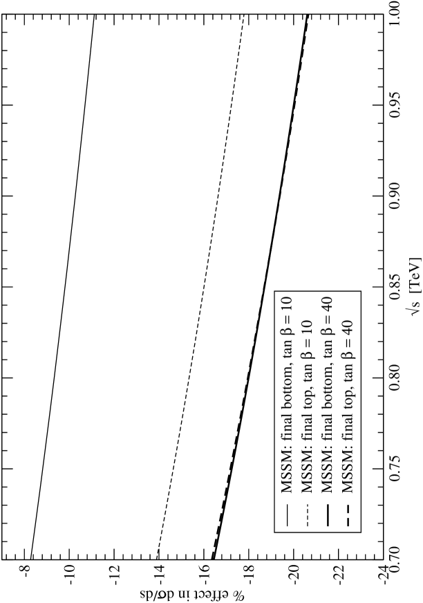
FIG. 6.: Effect of the combined electroweak and SUSY QCD corrections in the cross section for final bottom or top pairs at LHC. The various parameters are $\sqrt{S}$ = 14 TeV, $M_{SUSY}$ = 350 GeV and $p_{T,min}$ = 10 GeV. We show the results obtained with two values of the MSSM parameters $\tan\beta$.

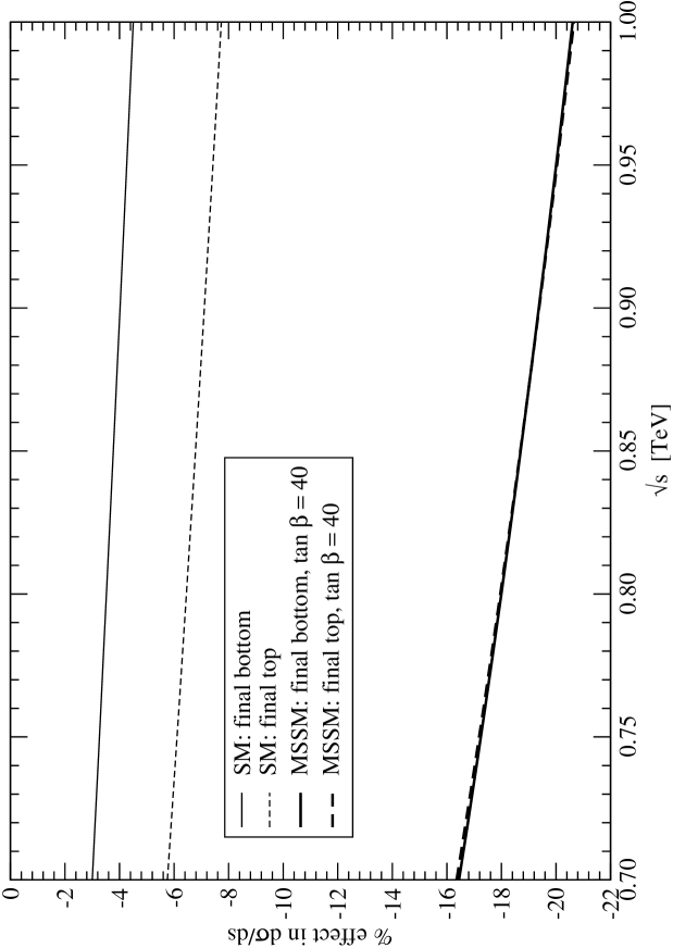
FIG. 7.: Comparison of the full effect in the Standard Model and in the MSSM. We show the correction to the cross section for final bottom or top pairs at LHC in the Standard Model and in the MSSM with $\tan\beta=40$. The other parameters are as in previous Figure: $\sqrt{S}$ = 14 TeV, $M_{SUSY}$ = 350 GeV and $p_{T,min}$ = 10 GeV.

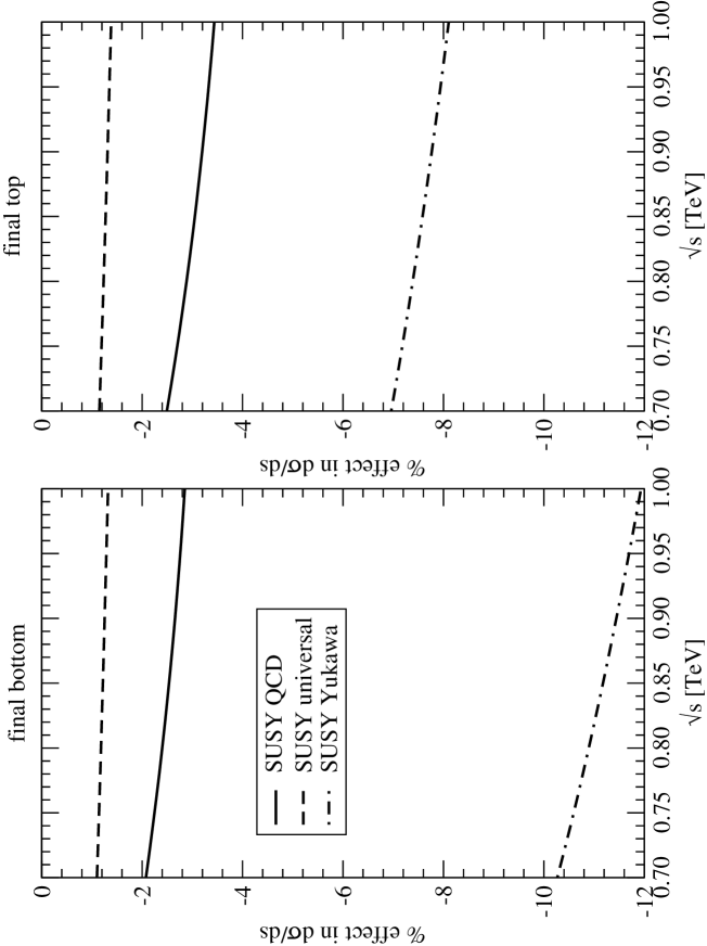
FIG. 8.: Separate SUSY effects. We show the three extra SUSY effects that are present in the MSSM with respect to the Standard Model. They are the SUSY component of the QCD correction, the universal SUSY electroweak terms and the $\tan\beta$ dependent SUSY Yukawa terms computed at $\tan\beta=40$. We recall that these genuine SUSY contributions grow like $\log s$. The other parameters are $\sqrt{S}$ = 14 TeV, $M_{SUSY}$ = 350 GeV and $p_{T,min}$ = 10 GeV.

REFERENCES

- [1] see e.g. R. Ströhmer, Acta Physica Polonica B33(2002)3887; T.Kamon, hep-ex/0301019, published in SUSY02, ”Hamburg 2002, Supersymmetry and Unification of fundamental Interactions, vol.1, p.138.
- [2] see e.g. D.P. Roy, hep-ph/0303106 and F.E. Paige, hep-ph/0307342.
- [3] The LEP Collaborations: ALEPH Coll, DELPHI Coll., L3 Coll., OPAL Coll., the LEP Electroweak Working Group, the SLD Heavy Flavor Working Group, hep-ex/0212036.
- [4] E. Maina, S. Moretti, M.R. Nolten and D.A. Ross, hep-ph/0307021, Phys .Lett. B570, (2003) 205.
- [5] P.Nason, G. Ridolfi, O. Schneider, G.F. Tartarelli and P. Vikas (conveners), in proceedings of the workshop on ”Standard Model Physics (and more) at the LHC”, Geneva 1999 (p.231-304) and references therein.
- [6] M. Beccaria, F. M. Renard and C. Verzegnassi, Phys. Rev. D64, 073008 (2001).
- [7] M. Beccaria, M. Melles, F. M. Renard and C. Verzegnassi, Phys.Rev.D65, 093007 (2002).
- [8] M. Beccaria, F.M. Renard and C. Verzegnassi, Phys. Rev. D63, 095010 (2001); Phys.Rev.D63, 053013 (2001);
- [9] M. Beccaria, M. Melles, F.M. Renard, S. Trimarchi, C. Verzegnassi, Int.Jour.Mod.Phys.A18,5069 (2003).
- [10] A. Castro, FERMILAB-CONF-02/213E(2002).
- [11] M. Beccaria, F.M. Renard, S. Trimarchi, C. Verzegnassi, Phys. Rev. D 68,035014 (2003).
- [12] see e.g. R.K. Ellis, W.J. Stirling and B.R. Webber, ”QCD and Colliders Physics”, Cambridge University Press, eds. T.Ericson and P.V. Landshoff (1996).
- [13] M. Ciafaloni, P. Ciafaloni and D. Comelli, Nucl.Phys.B589,359 (2000).
- [14] A. Denner, S. Pozzorini, Eur. Phys. J. C18,461 (2001.
- [15] M. Beccaria, F. M. Renard, C. Verzegnassi, Nucl.Phys. B663,394 (2003).
- [16] General information and updated numerical routines for parton distribution functions can be found on the www site http://durpdg.dur.ac.uk/hepdata/. The set we used is described in A.D. Martin, R.G. Roberts, W.J. Stirling, R.S. Thorne, “MRST partons and uncertainties”, contribution to XI International Workshop on Deep Inelastic Scattering, St. Petersburg, 23-27 April 2003, hep-ph/0307262.
- [17] M. Beccaria, P. Ciafaloni, D. Comelli, F.M. Renard, C. Verzegnassi, Phys. Rev. D 61,11301 (2000).
- [18] E. Accomando, A.R. Denner, S. Pozzorini, Phys. Rev. D65,073003 (2002).