Neutrino Masses and Oscillations:
Triumphs and Challenges

Abstract

The recent progress in establishing the existence of finite neutrino masses and mixing between generations of neutrinos has been remarkable, if not astounding. The combined results from studies of atmospheric neutrinos, solar neutrinos, and reactor antineutrinos paint an intriguing picture for theorists and provide clear motivation for future experimental studies. In this review, we summarize the status of experimental and theoretical work in this field and explore the future opportunities that emerge in light of recent discoveries.

1 Introduction and Historical Perpective

For almost 70 years, neutrinos have played a pivotal role in the the quest to understand elementary particles and their interactions. The neutrino was actually the first particle proposed by a theorist to guarantee the validity of a symmetry principle: Pauli boldly suggested [1] that neutrinos (invisible then and remaining so for another twenty five years) are emitted together with electrons in nuclear beta decay to salvage both energy and angular momentum conservation in the beta decay process. Experimental confirmation of Pauli’s hypothesis required many decades of experimental effort, but the discovery of the antineutrino in the fifties by Reines and Cowan [2] and subsequent experiments in the early sixties ultimately led to the Nobel Prizes for Reines (1995) and Lederman, Schwartz and Steinberger (1988). More recently, the 2002 Nobel prize was awarded to Davis and Koshiba for their seminal roles in the development of neutrino astrophysics (along with Giaconni for x-ray astrophysics).

The standard model of electroweak interactions, developed in the late 1960’s, provided a theoretical framework to incorporate the neutrinos as left-handed partners to the charged leptons, organized in two generations along with the quarks. The subsequent discovery of charmed quarks and the third generation of quarks and leptons completed the modern view of the standard model of electroweak interactions. This version possessed additional richness to incorporate CP violation, and further efforts to unify the strong interaction led to the development of Grand Unified Theories (GUTs). These GUTs provided a natural framework for nucleon decay and for neutrino masses, and motivated many experiments in the field.

Following on the successes of big-bang nucleosynthesis (BBN) and the discovery of the cosmic microwave background, it also became clear that neutrinos were potentially major players in the history of the early universe. The increasing evidence for the existence (and then dominance) of dark matter in the universe then led to the economical and seductive hypothesis that neutrinos, with small but finite mass, could provide the mass to explain the dark matter. This set the stage for a major experimental assault on the issue of neutrino mass and its role in cosmology, and provided substantial impetus to a worldwide program of experiments addressing the issues of finite neutrino mass and the possibility of mixing between generations.

Although it now appears that neutrinos are not likely the source of dark matter in the universe, the experimental evidence obtained in the last decade for finite neutrino masses and mixing between generations is strong and irrefutable. The pattern of masses and mixing angles emerging from the experiments provides an intriguing glimpse into the fundamental source of particle mass and the role of flavor in the scheme of particles and their interactions. The scale of neutrino mass differences motivates new experimental searches for double beta decay and end-point anomalies in beta decay, as well as new studies of oscillation phenomena using accelerators, nuclear reactors, and astrophysical sources of neutrinos.

In this review, we attempt to synthesize these themes, present a concise and coherent view of the experimental and theoretical developments leading to the current picture, and motivate the future explorations necessary to resolve the remaining issues . We begin with a summary of the theoretical motivation for studying neutrino masses and mixing, along with a development of the phenomenological framework for interpreting the experiments. This includes neutrino oscillations in vacuum as well as in matter, CP violation, ordinary beta decay, and double beta decay. We then review the recent experimental data that contribute to our present knowledge of these neutrino properties. We discuss the successful neutrino oscillation measurements, including the key contributions from various solar neutrino experiments, cosmic ray-induced atmospheric neutrino studies, and the recent dramatic results from the Sudbury Neutrino Observatory and the KamLAND reactor neutrino experiment. Important additional information is obtained from the experimental attempts that have thus far only yielded limits on neutrino masses such as double beta decay and tritium beta decay. We also will briefly discuss the role of massive neutrinos in cosmology, and the corresponding constraints.

The discussion of the future experimental program is separated into two different time scales. In the near-term future, the planned experiments will focus on a better determination of the mixing matrix parameters, in particular $\theta_{13}$, and resolution of the LSND puzzle (right or wrong). Further studies in the longer-term will of course depend on the outcome of these measurements, but there is substantial interest in pursuing the search for CP violation, the possibility that neutrinos are Majorana particles and other issues related to the mechanism(s) responsible for the observed phenomena.

2 Theoretical Framework

It is natural to expect that neutrinos have nonvanishing masses, since they are not required to be massless by gauge invariance or other symmetry principles. Moreover, all other known fermions, quarks and charged leptons, are massive. Nevertheless, neutrinos are very light, much lighter than the other fermions, and this striking qualitative feature needs to be understood, even though we do not know why e.g. the electron mass is what it is known to be, and why muons and taus are heavier than electrons.

The most popular explanation of the small neutrino masses is the “see-saw mechanism” [3] in which the neutrino masses are inversely proportional to some large mass scale $M_{\mathcal{H}}$. Simply put, if neutrinos are Majorana particles, i.e., indistiguishable from their own antiparticles, they have only two states, corresponding to the two possible spin orientations. On the other hand, Dirac particles, distinct from their antiparticles, have four states, two spin orientations for the particle and antiparticle. In the “see-saw mechanism” there are still four states for each neutrino family, but they are widely split by the “Majorana mass term” (explained later) into the two-component light neutrinos with masses $M_{\mathcal{L}}$ and the very heavy (sterile) two-component neutrinos with the mass $M_{\mathcal{H}}$, in such a way that $M_{\mathcal{L}}M_{\mathcal{H}}\cong M_{\mathcal{D}}^{2}$. Further, if we assume that the “Dirac mass” $M_{\mathcal{D}}$ is of the same order of magnitude as the Dirac fermion masses (masses of quarks and charged leptons), we can understand why $M_{\mathcal{L}}$ is so small, provided $M_{\mathcal{H}}$ is very large. If that explanation of the small neutrino mass is true, then the experimentally observed neutrinos are Majorana particles, and hence the total lepton number is not conserved. Observation of the violation of the total lepton number conservation (we explain further why it is difficult to observe it) would be a signal that neutrinos are indeed Majorana particles.

Neutrinos interact with other particles only by weak interactions (at least as far as we know); they do not have electromagnetic or color charges. That further distinguishes them from the other fermions which also interact electromagnetically (charged leptons and quarks) and strongly (quarks).

It is well known that the weak charged currents of quarks do not couple to a definite flavor state (or mass state), but to linear combinations of quark states. This phenomenon is described by the Cabibbo-Kobayashi-Maskawa (CKM) matrix, which by convention describes linear combinations of the charge $-e/3$ quark mass eigenstates $d,s,b$. The mixed states $d^{\prime},s^{\prime},b^{\prime}$, form weak doublets with the $u,c,t$ quark mass eigenstates. Consequently, the three generations of quark doublets are not independently preserved in charged-current weak processes.

An analogous situation is encountered with neutrinos. There, however, one can directly observe only the ‘weak eigenstates’, i.e., neutrinos forming weak charged currents with electrons, muons or tau . Information on the neutrino mixing matrix is best obtained by the study of neutrino oscillation, a quantum mechanical interference effect resulting from the mixing. As a consequence, like in quarks, the flavor (or family) is not conserved and, for example, a beam of electron neutrinos could, after travelling a certain distance, acquire a component of muon or tau flavor neutrinos. We describe the physics and formalism of the oscillations next. The formalism has been covered in great detail in numerous books and reviews. Thus, we restrict ourselves only to the most essential points. The interested reader can find more details in the monographs [4, 5, 6, 7, 8, 9, 10] and recent reviews [11, 12, 13, 14, 15, 16, 17, 18].

2.1 Neutrinos in the standard electroweak model

In the standard model individual lepton charges ($L_{e}=1$ for $e^{-}$ and $\nu_{e}$ and $L_{e}=-1$ for $e^{+}$, and $\bar{\nu}_{e}$ and analogously for $L_{\mu}$ and $L_{\tau}$) are conserved. Thus, processes such as $\mu^{+}\rightarrow e^{+}+\gamma$, or $K_{L}\rightarrow e^{\pm}+\mu^{\mp}$ are forbidden. Indeed, such processes have not been observed so far, and small upper limits for their branching ratios have been established.

Based on these empirical facts, the standard model places the left-handed components of the charged lepton and neutrino fields into the doublets of the group $SU(2)_{L}$,

$$\psi_{\ell L}=\left(\begin{array}[]{c}\nu_{\ell L}\\ \ell_{L}\end{array}\right)~{},~{}\ell=e,\mu,\tau~{},$$ (1)

while the right-handed components of the charged lepton fields are singlets. The right-handed components of the neutrino fields are absent in the standard electroweak model by definition.

As a consequence of this assignment, neutrinos are deemed to be massless, and the individual lepton numbers, as well as the total one, are strictly conserved. Note that with these assignments neutrino masses do not arise even from loop corrections. Thus, observation of neutrino oscillations, leading to the neutrino flavor nonconservation, signals deviations from this simple picture, and to the ‘physics beyond the standard model’.

Note also that studies of $e^{+}e^{-}$ annihilation at the $Z$-resonance peak have determined the invisible width of the $Z$ boson, caused by its decay into unobservable channels. Interpreting this width as a measure of the number of neutrino active flavors, one obtains $N_{\nu}=2.984\pm 0.008$ from the four LEP experiments [20]. We can, therefore, quite confidently conclude that there are just three active neutrinos with masses of less than $M_{Z}/2$. (The relation of this finding to the fact that there are also three flavors of quarks is suggestive, but so far not really understood.) Besides these three active neutrino flavors there could be other neutrinos which do not partipate in weak interactions. Such neutrinos are called ‘sterile’. In general, the active and sterile neutrinos can mix, and thus the sterile neutrino can interact, albeit with a reduced strength.

Big Bang Nucleosynthesis (BBN) is sensitive to the number of neutrino flavors which are ultrarelativistic at the ‘freezeout’ when the $n\leftrightarrow p$ reactions are no longer in equilibrium and therefore it is perhaps sensitive to (almost) sterile neutrinos. However, analysis of BBN (i.e., of the abundances of ⁴He, $d$, ³He, and ⁷Li) are consistent with 3 neutrinos, and disfavors $N_{\nu}=4$ for fully thermalized neutrinos [19].

2.2 Neutrino mass terms

In a field theory of neutrinos the mass is determined by the mass term in the Langrangian. Since the right-handed neutrinos are absent in the standard electroweak model, one can either generalize the model and define the mass term by using the ideas of the see-saw mechanism, or one can add more possibilities by adding to the three known neutrino fields $\nu_{\ell L}$ new fields, corresponding to possibly heavy right-handed neutrinos $\nu_{jR}$. The mass term is then constructed out of the fields $\nu_{\ell L}$, their charge-conjugated and thus right-handed fields $(\nu_{\ell L})^{c}$ and from the fields $\nu_{jR},(\nu_{jR})^{c}$. There are, in general, two types of mass terms,

$$-L_{M}={\mathcal{M}}_{i\ell}^{D}\bar{\nu}_{iR}\nu_{\ell L}+\frac{1}{2}{\mathcal{M}}_{ij}^{M}(\bar{\nu}_{iR})(\nu_{jR})^{c}+{\rm H.c.}~{}.$$ (2)

(The term with $\bar{\nu^{c}}_{\ell^{\prime}L}\nu_{\ell L}$ is left out assuming that the corresponding coefficients are vanishing or negligibly small.)

The first term is a Dirac mass term, analogous to the mass term of charged leptons. It conserves the total lepton number, but might violate the individual lepton flavor numbers.

The second term is a Majorana mass term which breaks the total lepton number conservation by two units. It is allowed only if the neutrinos have no additive conserved charges of any kind.

If there are 3 left handed neutrinos $\nu_{\ell L}$, and $n$ additional sterile neutrinos $\nu_{jR}$ it is convenient to define

$$\nu=\left(\begin{array}[]{c}\nu_{\ell L}\\ (\nu_{jR})^{c}\end{array}\right)~{},~{}~{}-L_{M}=\frac{1}{2}\bar{\nu^{c}}M_{\nu}\nu+{\rm H.c.}~{},~{}~{}M_{\nu}=\left(\begin{array}[]{cc}0&{\mathcal{M}}^{D}\\ ({\mathcal{M}}^{D})^{T}&{\mathcal{M}}^{M}\end{array}\right)~{}.$$ (3)

The matrix $M_{\nu}$ is a symmetric complex matrix and $\mathcal{M}^{T}$ is the transposed matrix. After diagonalization it has $3+n$ mass eigenstates $\nu_{k}$ that represent Majorana neutrinos $(\nu_{k}^{c}=\nu_{k})$.

From the point of view of phenomenology, there are several cases to be discussed. The seesaw mechanism corresponds to the case when the scale of ${\mathcal{M}}^{M}$ is very large. There are three light active Majorana neutrinos in that case.

On the other hand, if the scale of ${\mathcal{M}}^{M}$ is not too high when compared to the electroweak symmetry breaking scale, there could be more than three light Majorana neutrinos, mixtures of active and sterile. Finally, when ${\mathcal{M}}^{M}=0$ there are six massive Majorana neutrinos that merge to form three massive Dirac neutrinos. The unitary matrix diagonalizing the mass term is a $3\times 3$ matrix in that case. In these latter cases the ‘natural’ explanation of the lightness of neutrinos is missing.

We shall not speculate further on the pattern of the mass matrix, even though a vast literature exists on that subject (see e.g. [13] for a partial list of recent references). In the interesting case of $N$ light left-handed Majorana neutrinos, the mass matrix is determined by $N$ neutrino masses, $N(N-1)/2$ mixing angles, $(N-1)(N-2)/2$ CP violating phases common to Dirac and Majorana neutrinos, and $(N-1)$ Majorana phases that affect only processes which violate the total lepton number (for the discussion of these Majorana phases see e.g. [21]).

2.3 Neutrino oscillation in vacuum

As stated earlier, the neutrinos participating in the charged current weak interactions (the usual way neutrinos are observed and the only way their flavor can be discerned) are characterized by the flavor ($e,\mu,\tau$). But the neutrinos of definite flavor are not necessarily states of a definite mass. Instead, they are generally coherent superpositions of such states,

$$|\nu_{\ell}\rangle=\sum_{i}U_{\ell i}|\nu_{i}\rangle~{}.$$ (4)

When the standard model is extended to include neutrino mass, the mixing matrix $U$ is unitary.

In vacuum, the mass eigenstates propagate as plane waves. Leaving out the common phase, a beam of ultrarelativistic neutrinos $|\nu_{i}\rangle$ with energy $E$ at the distance $L$ acquires a phase

$$|\nu_{i}(L)\rangle\sim|\nu_{i}(L=0)\rangle\exp(-i\frac{m_{i}^{2}}{2}\frac{L}{E})$$ (5)

Given that, the amplitude of the process $\nu_{\ell}\rightarrow\nu_{\ell^{\prime}}$ is

$$A(\nu_{\ell}\rightarrow\nu_{\ell^{\prime}})=\sum_{i}U_{\ell i}e^{-i\frac{m_{i}^{2}L}{2E}}U_{\ell^{\prime}i}^{*}~{},$$ (6)

and the probability of the flavor change for $\ell\neq\ell^{\prime}$ is the square of this amplitude. It is obvious that due to the unitarity of $U$ there is no flavor change if all masses vanish or are exactly degenerate. The existence of the oscillations is a simple consequence of the coherence in Eq. (4). The detailed description of the quantum mechanics of the oscillations in terms of wave packets is subtle and a bit involved (see, e.g. the reviews [22] and references therein). It includes, among ather things, the concept of coherence length, a distance after which there is no longer coherence in Eq. (4). For the purpose of this review such issues are irrelevant, and will not be discussed further.

The idea of oscillations was discussed early on by Pontecorvo [23, 24] and by Maki, Nakagawa and Sakata [25]. Hence, the mixing matrix $U$ is often associated with these names and the notation $U_{MNS}$ or $U_{PMNS}$ is used.

The formula for the probability is particularly simple when only two neutrino flavors, $\nu_{\ell}$ and $\nu_{\ell^{\prime}}$, mix appreciably, since only one mixing angle is then relevant,

$$P(\nu_{\ell}\rightarrow\nu_{\ell^{\prime}\neq\ell})=\sin^{2}2\theta\sin^{2}\left[1.27\Delta m^{2}({\rm eV^{2}})\frac{L({\rm km})}{E_{\nu}({\rm GeV})}\right]~{},$$ (7)

where the appropriate factors of $\hbar$ and $c$ were included (the same is obtained when the length is in meters and energy in MeV). Here $\Delta m^{2}\equiv|m_{2}^{2}-m_{1}^{2}|$ (note that the sign is irrelevant) is the mass squared difference.

Thus, the oscillations in this simple case are characterized by the oscillation length

$$L_{osc}({\rm km})=\frac{2.48E_{\nu}{\rm(GeV)}}{\Delta m^{2}{\rm(eV^{2})}}~{},$$ (8)

and by the amplitude $\sin^{2}2\theta$.

For obvious reasons the oscillation studies are optimally performed at distances $L\sim L_{osc}$ from the neutrino source. At shorter distances the oscillation amplitude is reduced and at larger distances the neutrino flux is reduced making the experiment more difficult. Note that at distance $L\gg L_{osc}$ the oscillation pattern is smeared out and the oscillation probability (7) approaches $(\sin^{2}2\theta/2)$ and becomes independent of $\Delta m^{2}$.

The mixing matrix of 3 neutrinos is parametrized by three angles, conventionally denoted as $\theta_{12},\theta_{13},\theta_{23}$, one $CP$ violating phase $\delta$ and two Majorana phases $\alpha_{1},\alpha_{2}$. Using $c$ for the cosine and $s$ for the sine, we write $U$ as

$$\left(\begin{array}[]{c}\nu_{e}\\ \nu_{\mu}\\ \nu_{\tau}\end{array}\right)=\left(\begin{array}[]{ccc}c_{12}c_{13}&s_{12}c_{13}&s_{13}e^{-i\delta}\\ -s_{12}c_{23}-c_{12}s_{23}s_{13}e^{i\delta}&c_{12}c_{23}-s_{12}s_{23}s_{13}e^{i\delta}&s_{23}c_{13}\\ s_{12}s_{23}-c_{12}c_{23}s_{13}e^{i\delta}&-c_{12}s_{23}-s_{12}c_{23}s_{13}e^{i\delta}&c_{23}c_{13}\end{array}\right)\left(\begin{array}[]{r}e^{i\alpha_{1}/2}~{}\nu_{1}\\ e^{i\alpha_{2}/2}~{}\nu_{2}\\ \nu_{3}\end{array}\right)~{}.$$ (18)

By convention the mixing angle $\theta_{12}$ is associated with the solar neutrino oscillations, hence the masses $m_{1}$ and $m_{2}$ are separated by the smaller interval $\Delta m_{sol}^{2}$ (we shall assume, again by convention, that $m_{2}>m_{1}$) while $m_{3}$ is separated from the 1,2 pair by the larger interval $\Delta m_{atm}^{2}$, and can be either lighter or heavier than $m_{1}$ and $m_{2}$. The situation where $m_{3}>m_{2}$ is called ‘normal hierarchy’, while the ‘inverse hierarchy’ has $m_{3}<m_{1}$. Not everybody follows these conventions, so caution should be used when comparing the various results appearing in the literature.

The general formula for the probability that the “transition” $\ell\rightarrow\ell^{\prime}$ happens at $L$ is

$$P(\nu_{\ell}\rightarrow\nu_{\ell^{\prime}}) = |\sum_{i}U_{\ell i}U_{\ell^{\prime}i}^{*}e^{-i(m_{i}^{2}/2E)L}|^{2}$$ (19)

$$= \sum_{i}|U_{\ell i}U_{\ell^{\prime}i}^{*}|^{2}+\Re\sum_{i}\sum_{j\neq i}U_{\ell i}U_{\ell^{\prime}i}^{*}U_{\ell j}^{*}U_{\ell^{\prime}j}e^{i\frac{|m_{i}^{2}-m_{j}^{2}|L}{2E}}~{}.$$

Clearly, the probability (19) is independent of the Majorana phases $\alpha$. The oscillations described by the Eq.(19) violate the individual flavor lepton numbers, but conserve the total lepton number. The oscillation pattern is identical for Dirac or Majorana neutrinos.

The general formula can be simplified in several cases of practical importance. For 3 neutrino flavors, using the empirical fact that $\Delta m_{atm}^{2}\gg\Delta m_{sol}^{2}$ and considering distances comparable to the atmospheric neutrino oscillation length, only three parameters are relevant in the zeroth order, the angles $\theta_{23}$ and $\theta_{13}$ and $\Delta_{atm}\equiv\Delta m_{atm}^{2}L/4E_{\nu}$. However, corrections of the first order in $\Delta_{sol}\equiv\Delta m_{sol}^{2}L/4E_{\nu}$ should be also considered and are included below (some of the terms with $\Delta_{sol}$ are further reduced by the presence of the emipirically small $\sin^{2}2\theta_{13}$):

$$P(\nu_{\mu}\rightarrow\nu_{\tau}) \simeq \cos^{4}\theta_{13}\sin^{2}2\theta_{23}\sin^{2}\Delta_{atm}$$

$$- \Delta_{sol}\cos^{2}\theta_{13}\sin^{2}2\theta_{23}(\cos^{2}\theta_{12}-\sin^{2}\theta_{13}\sin^{2}\theta_{12})\sin 2\Delta_{atm}$$

$$- \Delta_{sol}\cos\delta\cos\theta_{13}\sin 2\theta_{12}\sin 2\theta_{13}\sin 2\theta_{23}\cos 2\theta_{23}\sin 2\Delta_{atm}/2$$

$$+ \Delta_{sol}\sin\delta\cos\theta_{13}\sin 2\theta_{12}\sin 2\theta_{13}\sin 2\theta_{23}\sin^{2}\Delta_{atm}~{},$$

$$P(\nu_{\mu}\rightarrow\nu_{e}) \simeq \sin^{2}2\theta_{13}\sin^{2}\theta_{23}\sin^{2}\Delta_{atm}$$

$$- \Delta_{sol}\sin^{2}\theta_{23}\sin^{2}\theta_{12}\sin^{2}2\theta_{13}\sin 2\Delta_{atm}$$

$$+ \Delta_{sol}\cos\delta\cos\theta_{13}\sin 2\theta_{13}\sin 2\theta_{23}\sin 2\theta_{12}\sin 2\Delta_{atm}/2$$

$$- \Delta_{sol}\sin\delta\cos\theta_{13}\sin 2\theta_{12}\sin 2\theta_{13}\sin 2\theta_{23}\sin^{2}\Delta_{atm}~{},$$

$$P(\nu_{\mu}\rightarrow\nu_{\mu})=1-P(\nu_{\mu}\rightarrow\nu_{e})-P(\nu_{\mu}\rightarrow\nu_{\tau})~{},$$ (22)

where $\delta$ is the $CP$ phase of Eq. (18) and

$$P(\nu_{e}\rightarrow\nu_{x}) \simeq \sin^{2}2\theta_{13}\left[\sin^{2}\Delta_{atm}-\Delta_{sol}\sin^{2}\theta_{12}\sin 2\Delta_{atm}\right]$$ (23)

$$+ \Delta^{2}_{sol}\cos^{4}\theta_{13}\sin^{2}2\theta_{12}~{},$$

where the term linear in $\Delta_{sol}$ is suppressed by the factor $\sin^{2}2\theta_{13}$ and therefore the quadratic term is also included. The $\nu_{e}$ disappearance probability is independent of the $CP$ phase $\delta$.

Note that the terms of first order in $\Delta_{sol}$ depend on the sign of $\Delta_{atm}$, i.e., on the hierarchy.

On the other hand, at distances much larger than the atmospheric neutrino oscillation length, the electron neutrino and antineutrino disappearance is governed by

$$P(\nu_{e}\rightarrow\nu_{x})\simeq 1-\sin^{4}\theta_{13}-\cos^{4}\theta_{13}\left[1-\sin^{2}2\theta_{12}\sin^{2}\Delta_{sol}\right]~{},$$ (24)

In both of the latter cases $\nu_{x}$ denotes any neutrino except $\nu_{e}$. (General expressions for mixing of three neutrinos in vacuum can be found in Eqs. (7)-(12) of Ref. [13].)

In the mixing matrix (18) the presence of the phase $\delta$ signifies the possibility of $CP$ violation, the expectation that

$$P(\nu_{\ell^{\prime}}\rightarrow\nu_{\ell})\neq P(\bar{\nu}_{\ell^{\prime}}\rightarrow\bar{\nu}_{\ell})~{},$$ (25)

i.e., that for example the probability of $\nu_{\mu}$ oscillating into $\nu_{e}$ is different from the probability of $\bar{\nu}_{\mu}$ oscillating into $\bar{\nu}_{e}$.

The magnitude of the $T$ or $CP$ violation is characterized by the differences

$$P(\bar{\nu}_{\mu}\rightarrow\bar{\nu}_{e})-P(\nu_{\mu}\rightarrow\nu_{e})=-[P(\bar{\nu}_{\mu}\rightarrow\bar{\nu}_{\tau})-P(\nu_{\mu}\rightarrow\nu_{\tau})]$$

$$= P(\nu_{e}\rightarrow\nu_{\tau})-P(\bar{\nu}_{e}\rightarrow\bar{\nu}_{\tau})$$

$$= -4c_{13}^{2}s_{13}c_{23}s_{23}c_{12}s_{12}\sin\delta[\sin 2\Delta_{12}+\sin 2\Delta_{23}+\sin 2\Delta_{31}]$$

$$= 16c_{13}^{2}s_{13}c_{23}s_{23}c_{12}s_{12}\sin\Delta_{12}\sin\Delta_{23}\sin\Delta_{31}~{},$$

where, as before, $\Delta_{ij}=(m_{i}^{2}-m_{j}^{2})\times L/4E$. Thus, the size of the effect is the same in all three channels, and $CP$ violation is observable only if all three masses are different (i.e., nondegenerate), and all three angles are nonvanishing. The possibility of $CP$ violation in the lepton sector was first discussed in [26, 27].

2.4 Neutrino oscillations in matter

The oscillation phenomenon has its origin in the phase difference between the coherent components of the neutrino flavor eigenstates described by Eq. (5). When neutrinos propagate in matter additional contributions to the phase appear, besides the one caused by the nonvanishing mass of the state $\nu_{i}$. To see the origin of such phase, consider the effective Hamiltonian of neutrinos in presence of matter. Obviously, only phase differences are of importance.

Without invoking any nonstandard interactions two effects are present. All active neutrinos interact with quarks and electrons by the neutral current weak interactions ($Z$ exchange), but only electron neutrinos and antineutrinos interact with electrons by the exchange of $W$. The corresponding effective potential is ($V_{C}$ stands for the charged current)

$$V_{C}(\nu_{e})=\sqrt{2}G_{F}N_{e}~{},~{}~{}{\rm and}~{}V_{C}(\bar{\nu}_{e})=-\sqrt{2}G_{F}N_{e}~{},$$ (27)

where $N_{e}$ is the electron number density. (There are no $\mu$ or $\tau$ leptons in normal matter, hence there is no analogous potential for $\nu_{\mu}$ or $\nu_{\tau}$.) In practical units

$$V_{C}=7.6Y_{e}\frac{\rho}{10^{14}{\rm(g/cm^{3})}}{\rm(eV)},~{}~{}Y_{e}=\frac{N_{e}}{N_{p}+N_{n}}~{}.$$ (28)

Similarly, any active neutrino acquires an effective potential due to the neutral-current interaction $V_{N}=-G_{F}N_{n}/\sqrt{2}$. The corresponding effective potential is absent for sterile neutrinos.

Given the effective potential, Eq.(27), electron neutrinos travelling distance $L$ in matter of constant density $N_{e}$ acquire an additional phase

$$\nu_{e}(L)=\nu_{e}(0)e^{-i\sqrt{2}G_{F}N_{e}L}~{}.$$ (29)

The corresponding matter oscillation length [28] is therefore

$$L_{0}=\frac{2\pi}{\sqrt{2}G_{F}N_{e}}~{}~{}\simeq\frac{1.7\times 10^{7}{\rm(m)}}{\rho{\rm(g/cm^{3})}~{}Y_{e}}~{}.$$ (30)

Unlike the vacuum oscillation length, Eq.(8), the matter oscillation length $L_{0}$ is independent of the neutrino energy. Note that the matter oscillation length in rock is $L_{0}\approx 10^{4}$ km, and in the center of the Sun $L_{0}\approx$ 200 km.

Considering for simplicity just two mass eigenstates $\nu_{1}$ and $\nu_{2}$ that are components of the flavor eigenstates $\nu_{e}$ and $\nu_{\alpha}$ with the mixing angle $\theta$, we obtain the time (or space) development Schrödinger equation

$$i\frac{d}{dt}\left(\begin{array}[]{c}\nu_{1}\\ \nu_{2}\end{array}\right)=\left(\begin{array}[]{cc}\frac{m_{1}^{2}}{2E}+V_{C}c^{2}&~{}~{}~{}~{}V_{C}sc\\ V_{C}sc&~{}~{}~{}~{}\frac{m_{2}^{2}}{2E}+V_{C}s^{2}\end{array}\right)\left(\begin{array}[]{c}\nu_{1}\\ \nu_{2}\end{array}\right)~{},$$ (37)

where, as before $c=\cos\theta$ and $s=\sin\theta$.

The $2\times 2$ matrix above can be brought to the diagonal form by the transformation

$$\nu_{1m} = \nu_{e}\cos\theta_{m}-\nu_{\alpha}\sin\theta_{m}$$ (38)

$$\nu_{2m} = \nu_{e}\sin\theta_{m}+\nu_{\alpha}\cos\theta_{m}~{},$$

where the new mixing angle in matter, $\theta_{m}$, depends on the vacuum mixing angle $\theta$ and on the vacuum and matter oscillation lengths $L_{osc}$ and $L_{0}$,

$$\tan 2\theta_{m}=\tan 2\theta\left(1-\frac{L_{osc}}{L_{0}\cos 2\theta}\right)^{-1}~{}.$$ (39)

The effective oscillation length in matter is then

$$L_{m}=L_{osc}\frac{\sin 2\theta_{m}}{\sin 2\theta}=L_{osc}\left[1+\left(\frac{L_{osc}}{L_{0}}\right)^{2}-\frac{2L_{osc}}{L_{0}}\cos 2\theta\right]^{-1/2}~{},$$ (40)

and the probability of detecting $\nu_{e}$ at a distance $L$ from the $\nu_{e}$ source has the usual form, but with $\theta\rightarrow\theta_{m}$ and $L_{osc}\rightarrow L_{m}$,

$$P(E_{\nu},L,\theta,\Delta m^{2})=1-\sin^{2}2\theta_{m}\sin^{2}\frac{\pi L}{L_{m}}~{}.$$ (41)

When considering oscillations with two flavors, the mixing angle $\theta$ can be restricted to the interval $(0,\pi/2)$. In vacuum, only $\sin^{2}2\theta$ is relevant, and hence only half of that interval, $(0,\pi/4)$ could be used. However, once matter oscillations are present, also the $\cos 2\theta$ becomes relevant, and thus the whole $(0,\pi/2)$ interval might be needed. The part of the parameter space corresponding to the $(\pi/4,\pi/2)$ angles was called the “dark” side in Ref.[32], who suggested using $\tan^{2}\theta$ in the plots instead of $\sin^{2}2\theta$. (The advantage of $\tan^{2}\theta$ is that when plotted on the log scale, the reflection symmetry around $\tan^{2}\theta=1$ for vacuum oscillations is maintained.) The importance of allowing the full range of the mixing angles in the three flavor analysis was stressed earlier, see e.g. Ref. [33].

With our convention $m_{2}>m_{1}$ mixing angles in the interval $(\pi/4,\pi/2)$ would mean that $\nu_{e}$ contains dominantly the heavier component $\nu_{2}$. (This is not the case in practice, see Sect. 3.1.) It appears now that at least two of the three mixing angle are large (and $\leq\pi/4$), and the constraint on the third one, $\theta_{13}$ are still such that linear plots are more revealing. Therefore, in the following we use the traditional plots with $\sin^{2}2\theta$.

The same results can be obtained, naturally, by rewriting the equation of motion in the flavor basis

$$i\frac{d}{dx}\left(\begin{array}[]{c}\nu_{e}\\ \nu_{\alpha}\end{array}\right)=2\pi\left(\begin{array}[]{cc}-\frac{\cos 2\theta}{L_{osc}}+\frac{1}{L_{0}}&\hskip 22.76228pt\frac{\sin 2\theta}{2L_{osc}}\\ \frac{\sin 2\theta}{2L_{osc}}&\hskip 22.76228pt0\end{array}\right)\left(\begin{array}[]{c}\nu_{e}\\ \nu_{\alpha}\end{array}\right)~{},$$ (48)

Here one can see clearly that in matter, unlike in vacuum, the oscillation pattern depends on whether the mixing angle $\theta$ is smaller or larger than $\pi/4$. (For antineutrinos the sign in front of $1/L_{0}$ is reversed.)

In matter of a constant density we can now consider several special cases:

• Low density limit, $L_{osc}\ll L_{0}$. In this case matter has a rather small effect. On Earth, one is able to observe oscillations only provided $L_{osc}<$ Earth diameter, and therefore this limit applies. The matter effects could be perhaps observed as small day-night variation in the solar neutrino signal. In long baseline oscillation experiments matter effects could cause difference in the oscillation probability of neutrinos and antineutrinos, hence these effects, together with the hierarchy problem (i.e., whether $m_{3}>m_{2}$ or $m_{3}<m_{1}$) are crucial in the search for $CP$ violation and its interpretation.

• High density limit, $L_{osc}\gg L_{0}$. The oscillation amplitude is suppressed by the factor $L_{0}/|L_{osc}|$. For $m_{2}^{2}>m_{1}^{2}$ the matter mixing angle is $\theta_{m}\rightarrow 90^{0}$ and thus $\nu_{e}\rightarrow\nu_{2}$.

• $|L_{osc}|\approx L_{0}$. In this case the matter effects can be enhanced. In particular, for $L_{osc}/L_{0}=\cos 2\theta$ one has $\sin^{2}2\theta_{m}=1$, i.e. the maximum mixing, even for small vacuum mixing angle $\theta$. This is the basis of the Mikheyev-Smirnov-Wolfenstein (MSW) effect [28, 34].

When neutrinos propagate in matter of varying density, the equations of motion (37) or (48) must be solved. There is a vast literature on the subject, in particular on the application to the solar neutrinos. There, the $\nu_{e}$ are often created at densities above the resonance density, and therefore are dominantly in the higher mass eigenstate. When the resonance density is reached, the two instantaneous eigenvalues are almost degenerate. In the adiabatic regime, the neutrino will remain in the upper eigenstate, and when it reaches vacuum it will be (for small vacuum mixing angle $\theta$) dominantly in the state that we denoted above as $\nu_{\alpha}$. In the general case, there is a finite probability $P_{x}$ for jumping from one eigenstate to the other one, and the conversion might be incomplete. The average survival probability is [35]

$$\langle P(\nu_{e}\rightarrow\nu_{e})\rangle=\frac{1}{2}[1+(1-2P_{x})\cos 2\theta_{m}(\rho_{max})\cos 2\theta]~{},$$ (49)

Usually $\cos 2\theta_{m}(\rho_{max})\simeq-1$ and thus $\langle P(\nu_{e}\rightarrow\nu_{e})\rangle\simeq\sin^{2}\theta+P_{x}\cos 2\theta$.

The transition point between the regime of vacuum and matter oscillations is determined by the ratio

$$\frac{L_{osc}}{L_{0}}=\frac{2\sqrt{2}G_{F}N_{e}E_{\nu}}{\Delta m^{2}}=0.22\left[\frac{E_{\nu}}{{\rm 1~{}MeV}}\right]\left[\frac{\rho Y_{e}}{{\rm 100g/cm^{3}}}\right]\left[\frac{7\times 10^{-5}{\rm eV^{2}}}{\Delta m^{2}}\right]$$ (50)

If this fraction is larger than unity, the matter oscillations dominate, and when this ratio is less than $\cos 2\theta$ the vacuum oscillations dominate. Generally, there is a smooth transition in between these two regimes.

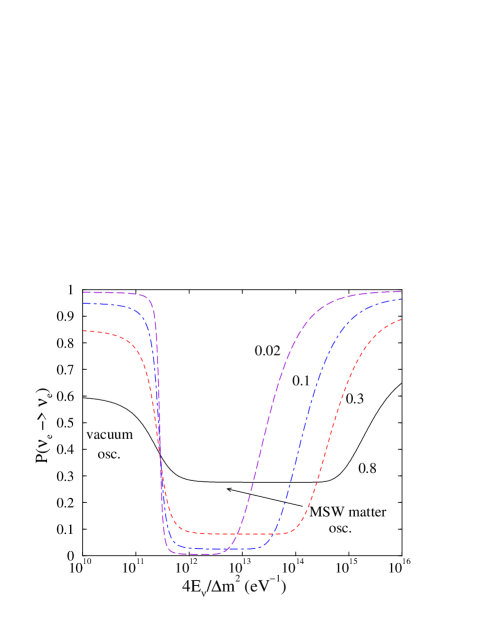
Figure 1: Schematic illustration of the survival probability of $\nu_{e}$ created at the solar center. The curves are labelled by the $\sin^{2}2\theta$ values.

The electron neutrino survival probability is illustrated in Fig. 1, where it is plotted against $4E_{\nu}/\Delta m^{2}$, see Eq.(50). In Fig. 1 it was assumed that the neutrinos originated in the center of the Sun, hence the relatively sharp feature at $4E_{\nu}/\Delta m^{2}\sim 2.6\times 10^{11}$ eV^-1 where according to the Eq.((50) $L_{osc}/L_{0}=1$ for the central density of the Sun. Note that below and above this dividing line the survival probability is almost independent of the neutrino energy, hence no spectrum distortion is expected. The subsequent increase in the neutrino survival probability for larger values of $4E_{\nu}/\Delta m^{2}$ is caused by the ‘nonadiabatic’ transition, i.e. by the gradual increase of the jump probability towards the limiting value $P_{x}\rightarrow 1$.

For the parameters corresponding to the preferred solar solution ($\sin^{2}2\theta\simeq 0.83$ and $\Delta m^{2}\sim 7\times 10^{-5}$ eV²) the $pp$ neutrinos with $4E_{\nu}/\Delta m^{2}<2.4\times 10^{10}$ eV^-1 and the ⁷Be neutrinos with $4E_{\nu}/\Delta m^{2}=4.9\times 10^{10}$ eV^-1 undergo vacuum oscillations, while the ⁸B neutrinos with $4E_{\nu}/\Delta m^{2}>2.55\times 10^{11}$ eV^-1 undergo MSW matter oscillations. (Clearly, that must be the case since otherwise it would be impossible to understand the $\sim$ 0.3 suppression of the ⁸B neutrino $\nu_{e}$ flux observed in the charged current reactions, see 3.1.)

2.5 Tests of CP, T and CPT invariance

In vacuum $CP$ conservation implies that $P(\nu_{\ell}\rightarrow\nu_{\ell^{\prime}})=P(\bar{\nu}_{\ell}\rightarrow\bar{\nu}_{\ell^{\prime}})$ (see Eq.(2.3). Violation of this inequality thus would mean that $CP$ is not conserved in the lepton sector. Substantial effort is devoted to the $CP$ tests. Matter effects can induce inequality between $P(\nu_{\ell}\rightarrow\nu_{\ell^{\prime}})$ and $P(\bar{\nu}_{\ell}\rightarrow\bar{\nu}_{\ell}^{\prime})$ and so the analysis must carefully account for them.

If $CP$ is not conserved, but $CPT$ invariance holds, then $T$ invariance will be also violated, i.e. $P(\nu_{\ell}\rightarrow\nu_{\ell^{\prime}})-P(\nu_{\ell^{\prime}}\rightarrow\nu_{\ell})$ need not vanish. Here matter effects cannot mimic the apparent $T$ invariance violation.

Finally, if $CPT$ is not conserved, then $P(\nu_{\ell}\rightarrow\nu_{\ell^{\prime}})-P(\bar{\nu}_{\ell^{\prime}}\rightarrow\bar{\nu}_{\ell})$ might be nonvanishing. Many tests of the $CPT$ invariance in the neutrino sector have been suggested, see e.g. [36] or references listed in [13].

$CPT$ invariance is based on Lorentz invariance, hermiticity of the Hamiltonian and locality. Its violation would have, naturally, enormous consequences. Yet there are many proposed scenarios of $CPT$ violation, in particular in the neutrino sector (for a whole series of papers on that topic see e.g. [37]).

$CPT$ invariance implies that neutrino and antineutrino masses are equal. If that is not true, then the $\Delta m^{2}$ as determined in the solar neutrino experiments (thus involving $\nu_{e}$) might not be the same as the $\Delta m^{2}$ needed to explain the LSND result which involves $\bar{\nu}_{\mu}\rightarrow\bar{\nu}_{e}$ oscillations, see 3.1.4 below. That was the gist of the phenomenological proposal in Ref. [38]. (See also further elaboration in [39].)

With the demonstration of the consistency between the observed solar $\nu_{e}$ deficit and the disappearance of reactor $\bar{\nu}_{e}$ by the KamLAND collaboration (see 3.1.3 below), this possibility seems unlikely, even though a proposal has been made to accommodate $CPT$ violation in that context [40], see also [42]. As has been shown in [41], the consistency of the solar $\nu$ oscillation solution and the KamLAND reactor result can be interpreted as a test of $CPT$ giving

$$|\Delta m_{\nu}^{2}-\Delta m_{\bar{\nu}}^{2}|<1.3\times 10^{-3}{\rm~{}eV^{2}}~{}~{}90\%{\rm~{}CL}~{},$$ (51)

where $\Delta m^{2}_{\nu}$ and $\Delta m^{2}_{\bar{\nu}}$ refer to the mass eigenstates $\nu_{1}$ and $\nu_{2}$ involved in the observed solar and reactor neutrino oscillations.

To test for the $CP$ invariance violation experimentally, one would compare the probabilities $P(\nu_{\mu}\rightarrow\nu_{e})$ and $P(\bar{\nu}_{\mu}\rightarrow\bar{\nu}_{e})$. This could be done realistically with $\sim$ 1 GeV $\nu_{\mu}$ beams at a distance $L\sim E_{\nu}/\Delta m_{atm}^{2}$ such that the contribution involving $\Delta m_{sol}^{2}$ are small. The effect of matter, however, must be included. Using the notation

$$s_{ij}=\sin\theta_{ij},~{}c_{ij}=\cos\theta_{ij},~{}\Delta_{ij}=\Delta m_{ij}^{2}L/4E_{\nu}$$ (52)

we obtain the formula

$$P(\nu_{\mu} \rightarrow \nu_{e})=4c_{13}^{2}s_{13}^{2}s_{23}^{2}\sin^{2}\Delta_{31}\hskip 199.16928pt$$ (53)

$$+ 8c_{13}^{2}s_{13}s_{23}c_{23}s_{12}c_{12}\sin\Delta_{31}[\cos\Delta_{32}\cos\delta-\sin\Delta_{32}\sin\delta]\sin\Delta_{21}$$

$$- 8c_{13}^{2}s_{13}^{2}s_{23}^{2}s_{12}^{2}\cos\Delta_{32}\sin\Delta_{31}\sin\Delta_{21}$$

$$+ 4c_{13}^{2}s_{12}^{2}[c_{12}^{2}c_{23}^{2}+s_{12}^{2}s_{23}^{2}s_{13}^{2}-2c_{12}c_{23}s_{12}s_{23}s_{13}\cos\delta]\sin^{2}\Delta_{21}$$

$$- 8c_{13}^{2}s_{13}^{2}s_{23}^{2}(1-2s_{13}^{2})\frac{aL}{4E_{\nu}}\sin\Delta_{31}\left[\cos\Delta_{32}-\frac{\sin\Delta_{31}}{\Delta_{31}}\right]~{}.$$

Here the first term gives the largest effect, while the terms in the third and fourth line represent small $CP$ conserving corrections (proportional to $\sin\Delta_{21}$ and $\sin^{2}\Delta_{21}$. The term with $\sin\delta$ in the second line violates $CP$ symmetry, while the term with $\cos\delta$ preserves it. Finally, the term with $aL/4E_{\nu}$ in the last line represents the matter effects.

The matter effects are characterized by

$$a=2\sqrt{2}G_{F}N_{e}E_{\nu}=1.54\times 10^{-4}Y_{e}\rho({\rm g/cm^{3}})E_{\nu}({\rm GeV})~{}(a~{}{\rm is~{}in~{}(eV^{2}))}.$$ (54)

The probability $P(\bar{\nu}_{\mu}\rightarrow\bar{\nu}_{e})$ is obtained by the substitution $\delta\rightarrow-\delta$ and $a\rightarrow-a$.

To test for $CP$ symmetry, one would determine

$$A_{CP} = \frac{P(\nu_{\mu}\rightarrow\nu_{e})-P(\bar{\nu}_{\mu}\rightarrow\bar{\nu}_{e})}{P(\nu_{\mu}\rightarrow\nu_{e})+P(\bar{\nu}_{\mu}\rightarrow\bar{\nu}_{e})}$$ (55)

$$\simeq -\Delta_{21}\frac{\sin 2\theta_{12}}{\sin\theta_{13}}\sin\delta-\frac{aL}{2E_{\nu}}\frac{\cos\Delta_{32}}{\sin\Delta_{31}}~{},$$

where we used the empirical fact that $\cos\theta_{23}\sim\sin\theta_{23}$ and $\sin(\Delta_{21})\sim\Delta_{21}$ for the distances and energies usually considered. Since $\theta_{13}$ is small, the $CP$ asymmetry can be enhanced. However, the individual terms in Eq. (55) depend on $\theta_{13}$, so for smaller $\theta_{13}$ it is more difficult to reach the required statistical precision.

There are several parameter degeneracies in Eq. (55) when separate measurements of $P(\nu_{\mu}\rightarrow\nu_{e})$ and $P(\bar{\nu}_{\mu}\rightarrow\bar{\nu}_{e})$ are made at given $L$ and $E_{\nu}$. ($i$) There can be two values $\delta,\theta_{13}$ and $\delta^{\prime},\theta_{13}^{\prime}$ leading to the same probabilities. $(ii)$ Sign of $\Delta_{31}$ and $\Delta_{32}$ (i.e. the normal or inverted hierarchy), where one set $\delta,\theta_{13}$ gives the same oscillation probabilities with one sign, as another set $\delta^{\prime},\theta_{13}^{\prime}$ with the opposite sign of $\Delta_{31}$.($iii$) Since the mixing angle $\theta_{23}$ is determined in experiments sensitive only to $\sin^{2}2\theta_{23}$ there is an ambiguity between $\theta_{23}$ and $\pi/2-\theta_{23}$. However, for the preferred value $\theta_{23}\sim\pi/4$ this ambiguity is essentially irrelevant. Various strategies to overcome the parameter degeneracies have been proposed. The choice of the neutrino energy $E_{\nu}$ (and whether a wide or narrow beam is used) and the distance $L$ play essential role. Clearly, if some of the so far unknown parameters (e.g. $\theta_{13}$ or the sign of the hierarchy) could be determined independently, some of these ambiguities would be diminished. (For some of the suggestions how to overcome the parameter degeneracy see e.g. [43, 44].)

2.6 Violation of the total lepton number conservation

Neutrino oscillations described so far are insensitive to the transformation properties under charge conjugation, i.e., whether neutrinos are Dirac or Majorana particles. However, if the mass eigenstates $\nu_{i}$ are Majorana particles, then $\nu\rightarrow\bar{\nu}$ oscillations that violate the total lepton number conservation are possible. There are two kinds of such processes.

Recall that in the standard Model charged current processes the neutrino $\nu_{\ell}$ produces the negatively charged lepton $\ell^{-}$ while antineutrino $\bar{\nu}_{\ell}$ produces the positively charged antilepton $\ell^{+}$. The standard model also requires that in order to produce the lepton $\ell^{-}$ the neutrino $\nu_{\ell}$ must have (almost) purely negative helicity, and similarly for $\ell^{+}$ the $\bar{\nu}_{\ell}$ must have (almost) purely positive helicity. The amplitudes for the ‘wrong’, i.e., suppressed helicity component is only of the order $m_{\nu}/E_{\nu}$ and therefore vanishes for massless neutrinos. But we know now that neutrinos are massive, although light, and the therefore ‘wrong’ helicity states are present.

When neutrinos are Majorana particles, the total lepton number may not be conserved. Thus, neutrinos $\nu_{\ell}$ born together with the leptons $\ell^{+}$ can create leptons $\ell^{+}$ (or even a different flavor $\ell^{\prime+}$) as long as the helicity rules are obeyed. The amplitude of this process is of the order $m_{\nu}/E_{\nu}$, thus small, independent of the distance the neutrinos travel. Therefore, this first kind of the $\nu\rightarrow\bar{\nu}$ transformation should not be really called oscillations. When such a transformation happens inside a nucleus, it leads to the process of neutrinoless double beta decay discussed in more detail below.

For Majorana neutrinos, there are several nonstandard processes involving helicity flip in which left-handed neutrinos $\nu_{L}$ are converted into right-handed (anti)neutrinos $\nu_{R}^{c}$. This can happen for Majorana neutrinos with a transition magnetic moment $\mu_{ij}$. In a transverse magnetic field $B_{\bot}$, $\nu_{iL}$ can be connected to $\nu_{jR}^{c}$. However, the transition probability is proportional to the small quantity $|\mu_{\nu}B|$ that vanishes for massless neutrinos. There are also models that predict neutrino decay involving a helicity-flip and a Majoron $\chi$ production. Again, the decay rate is expected to be small. If such processes exist one expects, among other things, that solar $\nu_{e}$ could be subdominantly converted into $\bar{\nu}_{e}$. The recent limit on the solar $\bar{\nu}_{e}$ flux, expressed as a fraction of the Standard Solar Model ⁸B $\nu_{e}$ flux is $2.8\times 10^{-3}$ [45]. (See also [45] for references to some of the theoretical model expectations for such $\nu\rightarrow\bar{\nu}$ conversion.)

In addition, there could be also transitions without helicity flip, which require that both Dirac and Majorana mass terms are present. These second class oscillations [46] involve transitions $\nu_{L}\rightarrow\nu^{c}_{L}$, i.e., the final neutrino is sterile and therefore unobservable. Estimates of the experimental observation possibilities of the neutrino-antineutrino oscillations are not encouraging [47].

Study of the neutrinoless double beta decay ($0\nu\beta\beta$) appears to be the best way to establish the Majorana nature of the neutrino, and at the same time gain valuable information about the absolute scale of the neutrino masses. Double beta decay is a rare transition between two nuclei with the same mass number $A$ involving change of the nuclear charge $Z$ by two units. The decay can proceed only if the initial nucleus is less bound than the final one, and both must be more bound than the intermediate nucleus. These conditions are fulfilled in nature for many even-even nuclei, and only for them. Typically, the decay can proceed from the ground state (spin and parity always $0^{+}$) of the initial nucleus to the ground state (also $0^{+}$) of the final nucleus, although the decay into excited states ($0^{+}$ or $2^{+}$) is in some cases also energetically possible. In Fig. 2 we show a typical situation for $A=136$. There are 11 candidate nuclei (all for the $\beta^{-}\beta^{-}$ decay) with $Q$ value above 2 MeV, thus potentially useful for the study of the $0\nu\beta\beta$ decay. (Large $Q$ values are preferable since the rate scales like $Q^{5}$ and the background suppression is typically easier for larger $Q$.)

Figure 2: Masses of nuclei with $A$ = 136. The even-even and odd-odd nuclei are connected by dotted lines. ¹³⁶Xe is stable against ordinary $\beta$ decay, but unstable against $\beta^{-}\beta^{-}$ decay. The same is true for ¹³⁶Ce, however, the $\beta^{+}\beta^{+}$ decay is expected to be slower than the $\beta^{-}\beta^{-}$ decay.

There are two modes of the double beta decay. The two-neutrino decay, $2\nu\beta\beta$,

$$(Z,A)\rightarrow(Z+2,A)+e_{1}^{-}+e_{2}^{-}+\bar{\nu}_{e1}+\bar{\nu}_{e2}$$ (56)

conserves not only electric charge but also lepton number. On the other hand, the neutrinoless decay,

$$(Z,A)\rightarrow(Z+2,A)+e_{1}^{-}+e_{2}^{-}$$ (57)

violates lepton number conservation. One can distinguish the two decay modes by the shape of the electron sum energy spectra, which are determined by the phase space of the outgoing light particles. Since the nuclear masses are so much larger than the decay $Q$ value, the nuclear recoil energy is negligible, and the electron sum energy of the $0\nu\beta\beta$ is simply a peak at $T_{e1}+T_{e2}=Q$ smeared only by the detector resolution.

The $2\nu\beta\beta$ decay is an allowed process with a very long lifetime $\sim 10^{20}$ years. It has been observed now in a number of cases [12]. Observing the $2\nu\beta\beta$ decay is important not only as a proof that the necessary background suppression has been achieved, but also allows one to constrain the nuclear models needed to evaluate the corresponding nuclear matrix elements.

The $0\nu\beta\beta$ decay involves a vertex changing two neutrons into two protons with the emission of two electrons and nothing else. One can visualize it by assuming that the process involves the exchange of various virtual particles, e.g. light or heavy Majorana neutrinos, right-handed current mediating $W_{R}$ boson, SUSY particles, etc. No matter what the vertex is, the $0\nu\beta\beta$ decay can proceed only when neutrinos are massive Majorana particles [48]. In the following we concentrate on the case when the $0\nu\beta\beta$ decay is mediated by the exchange of light Majorana neutrinos interacting through the left-handed $V-A$ weak currents. The decay rate is then,

$$[T_{1/2}^{0\nu}(0^{+}\rightarrow 0^{+})]^{-1}~{}=~{}G^{0\nu}(E_{0},Z)\left|M_{GT}^{0\nu}-\frac{g_{V}^{2}}{g_{A}^{2}}M_{F}^{0\nu}\right|^{2}\langle m_{\beta\beta}\rangle^{2}~{},$$ (58)

where $G^{0\nu}$ is the exactly calculable phase space integral, $\langle m_{\beta\beta}\rangle$ is the effective neutrino mass and $M_{GT}^{0\nu}$, $M_{F}^{0\nu}$ are the nuclear matrix elements.

The effective neutrino mass is

$$\langle m_{\beta\beta}\rangle=|\sum_{i}|U_{ei}|^{2}m_{\nu_{i}}e^{i\alpha_{i}}|~{},$$ (59)

where the sum is only over light neutrinos ($m_{i}<10$ MeV). The Majorana phases $\alpha_{i}$ were defined earlier in Eq.(18). If the neutrinos $\nu_{i}$ are $CP$ eigenstates, $\alpha_{i}$ is either 0 or $\pi$. Due to the presence of these unknown phases, cancellation of terms in the sum in Eq.(59) is possible, and $\langle m_{\beta\beta}\rangle$ could be smaller than any of the $m_{\nu_{i}}$.

The nuclear matrix elements, Gamow-Teller and Fermi, appear in the combination

$$M_{GT}^{0\nu}-\frac{g_{V}^{2}}{g_{A}^{2}}M_{F}^{0\nu}\equiv\langle f|\sum_{lk}H(r_{lk},\bar{E}_{m})\tau_{l}^{+}\tau_{k}^{+}\left(\vec{\sigma}_{l}\cdot\vec{\sigma}_{k}-\frac{g_{V}^{2}}{g_{A}^{2}}|i\rangle\right)~{}.$$ (60)

The summation is over all nucleons, $|i\rangle,(|f\rangle)$ are the initial (final) nuclear states, and $H(r_{lk},\bar{E}_{m})$ is the ‘neutrino potential’ (Fourier transform of the neutrino propagator) that depends (essentially as $1/r$) on the internucleon distance. When evaluating these matrix elements the short-range nucleon-nucleon repulsion must be taken into account due to the mild emphasis on small nucleon separations.

There is a vast literature devoted to the evaluation of these nuclear matrix elements, going back several decades. It is beyond the scope of the present review to describe this effort in detail. The interested reader can consult various reviews on the subject, e.g. [12, 49, 50].

Obviously, any uncertainty in the nuclear matrix elements is reflected as a corresponding uncertainty in the $\langle m_{\beta\beta}\rangle$. There is, at present, no model independent way to estimate the uncertainty, and to check which of the calculated values are correct. Good agreement with the known $2\nu\beta\beta$ is a necessary but insufficient condition. The usual guess of the uncertainty is the spread, by a factor of $\sim 3$, of the matrix elements calculated by different authors. Clearly, more reliable evaluation of the nuclear matrix element is a matter of considerable importance. (For a recent attempt to reduce and understand the spread of the calculated values, see [51].)

The $0\nu\beta\beta$ decay is not the only possible observable manifestation of lepton number violation. Muon-positron conversion,

$$\mu^{-}+(A,Z)\rightarrow e^{+}+(A,Z-2)~{},$$ (61)

or rare kaon decays $K_{\mu\mu\pi},~{}K_{ee\pi}$ and $K_{\mu e\pi}$,

$$K^{+}\rightarrow\mu^{+}\mu^{+}\pi^{-}~{},K^{+}\rightarrow e^{+}e^{+}\pi^{-}~{},K^{+}\rightarrow\mu^{+}e^{+}\pi^{-}~{},$$ (62)

are examples of processes that violate total lepton number conservation and where good limits on the corresponding branching ratios exist. (See Ref. [52] for a more complete discussion.) However, it appears that the $0\nu\beta\beta$ decay is, at present, the most sensitive tool for the study of the Majorana nature of neutrinos.

2.7 Direct measurement of neutrino mass

Conceptually the simplest way to explore the neutrino mass is to determine its effect on the momenta and energies of charged particles emitted in weak decays.

In two-body decays, e.g. $\pi^{+}\rightarrow\mu^{+}+\nu_{\mu}$ the analysis is particularly straightforward, at least in principle. In the system where the decaying pion is at rest, the energy and momentum conservation requirements mean that

$$m_{\nu}^{2}=m_{\pi}^{2}+m_{\mu}^{2}-2m_{\pi}\sqrt{m_{\mu}^{2}+p_{\mu}^{2}}~{}.$$ (63)

However, the neutrino mass squared appears as a difference of two very large numbers. Hence the uncertainties in $m_{\pi},p_{\mu}$ and even $m_{\mu}$ mean that the corresponding mass limit is only $m_{\nu}<170$ keV.

This problem can be avoided by studying the three body decays, in particular the nuclear beta decay. Near the endpoint of the beta spectrum a massive neutrino has so little kinetic energy that the effects of its finite mass become more visible. The electron spectrum of an allowed beta decay is given by the corresponding phase-space factor

$$\frac{dN}{dE}\sim F(Z,E_{e})p_{e}E_{e}(E_{0}-E_{e})[(E_{0}-E_{e})^{2}-m_{\nu}^{2}]^{1/2}~{},$$ (64)

where $E_{e},p_{e}$ is the electron energy and momentum and $F(Z,E_{e})$ describes the Coulomb effect on the outgoing electron. The quantity $E_{0}$ is the endpoint energy, the difference of total energies of the initial and final systems. Clearly, the effect of finite neutrino mass becomes visible if $(E_{0}-E_{e})\sim m_{\nu}$, i.e. very near the threshold.

For the case of several massive neutrinos with mixing, the beta decay spectrum is an incoherent superposition of spectra like (64) with corresponding weights $|U_{ei}|^{2}$ for each mass eigenstate $m_{\nu_{i}}^{2}$. If the experiment has insufficient energy resolution the quantity

$$m_{\nu_{e}}^{2{\rm(eff)}}=\sum_{i}|U_{ei}|^{2}m_{\nu_{i}}^{2}$$ (65)

(using the RPP notation [20]) could be determined from the electron spectrum near its endpoint, where the sum is over all the experimentally unresolved neutrino masses $m_{\nu_{i}}$.

Based on an upper limit for the $m_{\nu_{e}}^{2{\rm(eff)}}$ one can deduce several limits that do not depend on the mixing parameters $|U_{ei}|^{2}$. First, at least one of the neutrinos (i.e. the one with the smallest mass) has a mass less or equal to that limit, $m^{2}_{\nu_{min}}\leq m^{2{\rm(eff)}}_{\nu_{e}}$. Moreover, if all (with an emphasis on all) $|\Delta m_{ij}^{2}|$ values are known, an upper limit of all neutrino masses is $m_{\nu_{max}}^{2}\leq m^{2{\rm(eff)}}_{\nu_{e}}+\sum_{i<j}|\Delta m_{ij}^{2}|$. Thus, if we assume that the $|\Delta m_{ij}^{2}|$ values deduced from the experiments on solar (and reactor) and atmospheric oscillation studies (and include also the LSND result) cover all possibilities, and combine that knowledge with the $m_{\nu_{e}}^{2{\rm(eff)}}$ limit from tritium beta decay, we may conclude that no active neutrinos with mass more than ‘a few’ eV exists.

3 Experimental Results and Interpretation

Positive evidence for neutrino mass has so far been obtained only in measurements of neutrino oscillations. As noted above in 2.3, the neutrino masses enter only through the differences in squared masses (i.e., $\Delta m_{ij}^{2}=m_{i}^{2}-m_{j}^{2}$), so although these measurements provide lower limits to the mass values (e.g., $m_{i}^{2}\geq\Delta m_{ij}^{2}$) they do not actually determine the masses. As discussed in 2.6 and 2.7, direct neutrino mass measurements and neutrinoless double beta decay allow determination of quantities related to the values of the masses themselves (as opposed to differences). However, these experiments have so far yielded only limits. Finally, additional constraints have been derived from measurements of the cosmic microwave background radiation and galaxy distribution surveys through the effect of neutrinos on the distribution of matter in the early universe. In this section, we summarize the positive observations from oscillation measurements followed by brief discussion of the direct measurements, double beta decay searches, and recent constraints from cosmology.

3.1 Neutrino Oscillation Results

The first hints that neutrino oscillations actually occur were serendipitously obtained through early studies of solar neutrinos and neutrinos produced in the atmosphere by cosmic rays (“atmospheric neutrinos”). In fact, the atmospheric neutrino measurements were a byproduct of the search for proton decay using large water Čerenkov detectors. So it is somewhat ironic that although there was substantial interest in searching for neutrino oscillations, the first evidence for this phenomena came from experiments designed for very different purposes.

As shown below, recent studies definitively establish that the solar neutrino flux is reduced due to flavor oscillations, and so it is now clear that the first real signal of neutrino oscillations was the long-standing deficit of solar neutrinos observed by Ray Davis and collaborators using the Chlorine radiochemical experiment in the Homestake mine. While it took almost three decades to demonstrate the real origin of this deficit, the persistent observations by Davis et al. and many other subsequent solar-$\nu$ experiments were actually indications of neutrino oscillations. We will discuss this subject in more detail below.

3.1.1 Atmospheric Neutrinos

The Kamiokande experiment in Japan [53] and the IMB experiment in the US [54]were pioneering experimental projects to develop large volume water Čerenkov detectors with the primary goal of detecting nucleon decay, as predicted by Grand Unified Theories developed in the 1970’s [55]. Although these detectors were located deep underground to avoid cosmic ray-induced background, they both encountered the potential background events produced by atmospheric neutrinos (both $\nu_{e}$ and $\nu_{\mu}$) that easily penetrated to these subterranean labs and (rarely) produced energetic events in the huge detectors. And indeed, both experiments [56, 57, 58] (along with the Soudan experiment [59]) observed that the ratio of $\nu_{\mu}$-induced events to $\nu_{e}$-induced events was substantially reduced from the expected value of $\sim 2$. The decay chain of $\pi^{\pm}$ produced in the upper atmosphere would produce (through the subsequent $\mu$-decay) a $\nu_{\mu}$, $\bar{\nu}_{\mu}$, and a $\nu_{e}$ (or $\bar{\nu}_{e}$). Thus, based on rather simple basic arguments one expects the ratio of $\nu_{\mu}$/$\nu_{e}$ events to be about $\sim 2$ - and this is supported by more detailed Monte Carlo simulations. The observed values were closer to $\sim 1$, which was viewed as an anomaly for many years. Here again, although $\nu$-oscillations could clearly cause this anomaly there was not enough corroborative evidence to substantiate this explanation.

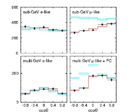
Figure 3: Distribution of observed atmospheric neutrino events vs. zenith angle from the SuperKamiokande experiment, compared with Monte Carlo simulations [60]. The blue hatched region represents the prediction without neutrino oscillations and the red line includes the effect neutrino oscillations. (PC means ‘partially contained’ events.)

However, the situation dramatically changed in 1998 when the larger experiment, Super-Kamiokande, reported a clearly anomalous zenith angle dependence of the $\nu_{\mu}$ events [61]. The measurements indicated a deficit of upward-going $\nu_{\mu}$-induced events (produced $\sim 10^{4}$ km away at the opposite side of the earth) relative to the downward-going events (produced $\sim 20$ km above). The $\nu_{e}$ events displayed a normal zenith angle behavior consistent with Monte Carlo simulations. Since at that time (1998) the solar-$\nu$ problem was still unresolved, these data represent the first really solid evidence for $\nu$-oscillations. More recent measurements [60] are displayed in Fig. 3, and the conclusion that flavor oscillations are responsible is essentially inescapable. Moreover, the deduced values of $\sin^{2}2\theta>0.90$ (90% C.L.) indicate a surprisingly strong mixing scenario where the muon-type neutrino seems to be a fully-mixed superposition of all three mass eigenstates. (This situation is completely contrary to the quark sector, where the mixing between generations is generally small.) The most recently reported value of $\Delta m^{2}$ derived from the Super-Kamiokande results is 0.0020 eV² [62] (for the error bars, see Table 1).

The observation of the angular distribution of upward-going muons produced by atmospheric neutrinos in the rock below the MACRO detector [63] supports the conclusion that the observed effect is due to the $\nu_{\mu}\rightarrow\nu_{\tau}$ oscillations, and disfavors $\nu_{\mu}\rightarrow\nu_{sterile}$ assignment.

Although the parallel effort to detect neutrino disappearance at nuclear reactors had made steady progress (setting upper limits and establishing exclusion plots) for many years, these experiments made a strong contribution at this point: the failure to observe $\bar{\nu}_{e}$ disappearance at CHOOZ [64] and Palo Verde [65] in the region near $\Delta m^{2}\simeq 0.0020~{}$eV² implies that the $\nu_{\mu}$ disappearance observed by Super-Kamiokande does not involve substantial $\nu_{e}$ appearance. (This inference assumes that $m_{\nu}=m_{\bar{\nu}}$ for each eigenstate as required by $CPT$ invariance.) Thus, it would seem that the $\nu_{\mu}$’s must be oscillating into $\nu_{\tau}$ or other more exotic particles, such as “sterile” neutrinos.

3.1.2 Solar Neutrinos

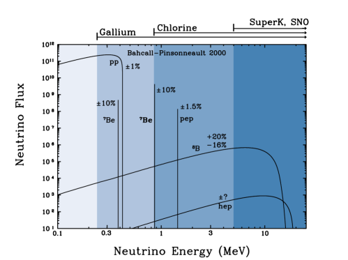
Figure 4: Energy distribution of the flux of solar neutrinos predicted by the standard solar model [66], as computed by J. Bahcall [67]. The ranges of energies associated with the various experiments are indicated at the top of the figure.

The interpretation of solar neutrino measurements involves substantial input from solar physics and the nuclear physics involved in the complex chain of reactions that together are termed the “Standard Solar Model” (SSM) [66] . The predicted flux of solar neutrinos from the SSM is shown in Fig. 4 as a function of neutrino energy. The low energy $p$-$p$ neutrinos are the most abundant and, since they arise from reactions that are responsible for most of the energy output of the sun, the predicted flux of these neutrinos is constrained very precisely ($\pm 2\%$) by the solar luminosity. The higher energy neutrinos are more accessible experimentally, but the fluxes are less certain due to uncertainties in the nuclear and solar physics required to compute them.

The early measurements included radiochemical experiments sensitive to integrated $\nu_{e}$ flux such as the Chlorine [68] (threshold energy 0.814 Mev) and Gallium [69] (0.233 MeV) experiments. Live counting was developed by the Kamiokande [70] and then the SuperKamiokande [71] experiments, based on neutrino-electron scattering, enabling measurements of both the flux and energy spectrum. Together these experiments sampled the solar neutrino flux over a wide range of energies. As can be seen in Fig. 8 below, all these experiments reported a substantial deficit in neutrino flux relative to the SSM. While it was realized that neutrino oscillations could be an attractive solution to this problem, it was problematic to establish this explanation with certainty due to the dependence on the SSM, its assumptions, and sensitivity to input from nuclear and solar physics.

However, it is now clear that the precise measurements of solar neutrino fluxes over a range of energies coupled with the amazing flavor transformation properties of neutrinos validates the SSM in a beautiful and satisfying manner. The solar-$\nu$ experiments and the SSM have been reviewed in detail elsewhere [20], and so it is not appropriate to repeat the details here. We present these solar neutrino flux measurements together in Fig. 8, where we also display the excellent agreement with the best fit solution to the combined solar-$\nu$ and KamLAND reactor data [72] to demonstrate the remarkably coherent picture that is strongly supported by these impressive experimental measurements and the associated SSM input.

3.1.3 SNO and KamLAND

With the advent of the new millenium, the stage was set for a synthesis of the study of solar neutrinos using a powerful new water Čerenkov detector (Sudbury Neutrino Observatory, SNO) with the study of the disappearance of reactor antineutrinos using a large scintillation detector located deep underground (KamLAND). The results of these experiments provide definitive evidence that the solar deficit is indeed due to flavor oscillations, and that this effect is demonstrable in a “laboratory” experiment on earth.

The SNO experiment combines the now high-developed capability of water Čerenkov detectors with the unique opportunities afforded by using deuterium to detect the solar neutrinos [73, 74]. Low energy neutrinos can dissociate deuterium via the charged current (CC) reaction

$$\nu_{e}+d\rightarrow e^{-}+2p$$ (66)

or the neutral current (NC) reaction

$$\nu_{\ell}+d\rightarrow\nu_{\ell}+p+n\>.$$ (67)

Only $\nu_{e}$ can produce the CC reaction, but all flavors $\ell=e,\mu,\tau$ can contribute to the NC rate. The CC reaction is detected via the energetic spectrum of $e^{-}$ which closely follows the ⁸B solar $\nu_{e}$ spectrum. The NC reaction involves three methods for detection of the produced neutron: (a) capture on deuterium and detection of the 6.25 MeV $\gamma$-ray, (b) capture on Cl (due to salt added to the D₂O) and detection of the 8.6 MeV $\gamma$-ray, or (c) capture in ³He proportional counters immersed in the detector. There are also some events associated with the elastic scattering of the solar-$\nu$ on $e^{-}$ in the detector which is dominated by the charged current reaction (again only $\nu_{e}$) but has some $\sim 20\%$ contribution from neutral currents (all flavors equally contribute).

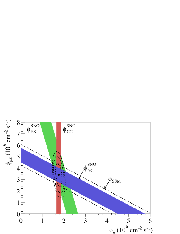
Figure 5: Measured solar neutrino fluxes from SNO for the NC and CC processes [74], along with elastic scattering events (ES) and the SSM prediction [66].

The SNO collaboration has published data on the CC and NC rate (from processes (a) and (b)). Additional data from the NC process (c) will be forthcoming in the future. Nevertheless, the reported results (see Fig. 5) demonstrate very clearly that the total neutrino flux ($\nu_{e}+\nu_{\mu}+\nu_{\tau}$ as determined from NC) is in good agreement with the SSM, but that the $\nu_{e}$ flux is suppressed (as determined from CC). This represents rather definitive evidence that the $\nu_{e}$ suppression is due to flavor-changing processes that convert the $\nu_{e}$ to the other flavors, as expected from $\nu$-oscillations. Furthermore, the observed value of $\nu_{e}$ flux and the observed energy spectrum, when combined with the other solar-$\nu$ measurements strongly favor another large mixing angle scenario at a lower value of $\Delta m^{2}\sim 10^{-5}$ eV².

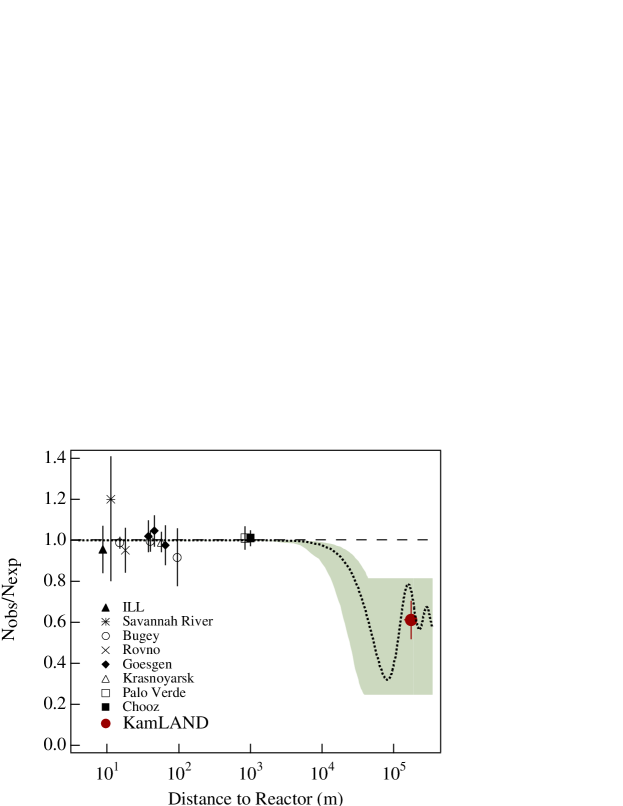
Figure 6: Ratio of observed to expected rates (without neutrino oscillations) for reactor neutrino experiments as a function of distance, including the recent result from the KamLAND experiment [75]. The shaded region is that expected due to neutrino oscillations with large mixing angle parameters as determined from solar neutrino data.

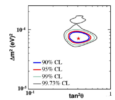
Figure 7: Region of parameter space constrained by simultaneous fit to solar-$\nu$ and KamLAND data, from [72]. The best fit values are $\Delta m^{2}=7.1\times 10^{-5}$ eV² and $\tan^{2}\theta=0.41$.

The KamLAND experiment [75] represents a major advance in the development of reactor $\bar{\nu}_{e}$ measurements. In order to reach the low values of $\Delta m^{2}\sim 10^{-5}$ eV² indicated by the solar-$\nu$ data, distances of order $\sim 200$ km are necessary (given the fixed range of $\bar{\nu}_{e}$ energies from reactors). The loss of rate due to $1/r^{2}$ scaling is severe, which requires substantial increases in source strength (i.e., reactor power) and detector size. Such a huge detector, sensitive to low-energy inverse beta-decay events from reactor $\bar{\nu}_{e}$, would be very susceptible to background from cosmic radiation and so must be located deep underground. By fortunate coincidence, the old Kamiokande site in Japan is very deep ($\sim 1000$ mwe) and located an average distance of $\sim 200$ km from a substantial number of large nuclear power reactors. Thus the KamLAND experiment, a large liquid scintillator detector, was built at this site to study the disappearance of $\bar{\nu}_{e}$ from nuclear reactors. For the first time in the long history of reactor $\bar{\nu}_{e}$ experiments (dating back to the original discovery of the $\bar{\nu}_{e}$ by Reines and Cowan [2]) a substantial deficit in event rate was observed (Fig. 6). In fact this deficit is just as predicted by the solar solution to the solar-$\nu$ oscillation solution, and the more precisely constrained values of $\Delta m^{2}$ and $\sin^{2}2\theta$ from a global analysis of the solar-$\nu$ and KamLAND data are shown in Fig. 7.

As mentioned previously, Fig. 8 shows a summary of the solar-$\nu$ data compared with the SSM with and without neutrino oscillations. The plotted experiments are: Ga, combined Gallium measurements from GALLEX and SAGE [69]; Cl, Chlorine measurement from Homestake mine [68]; SNO, Sudbury Neutrino Observatory (CC and NC)[72, 73, 74]; and SK, Super-Kamiokande[71]. In this plot one can clearly see the decreasing survival fraction with increasing energy in the progression Ga$\rightarrow$Cl$\rightarrow$SNO_CC (all sensitive only to the $\nu_{e}$ component). The SNO_NC measurement shows no suppression, whereas the SK data exhibit the intermediate suppression due to the partial contribution of NC events to their elastic scattering signal.

In summary, the experimental studies of solar neutrinos, atmospheric neutrinos, and reactor antineutrinos have established neutrino oscillations with two different mass scales, $\Delta m^{2}\sim 2.0\times 10^{-3}$ eV² and $\Delta m^{2}\sim 7.1\times 10^{-5}$ eV², both with large associated mixing angles. The allowed regions are shown in Fig. 9, and together these experiments constrain many of the matrix elements in the $3\times 3$ mixing matrix for the neutrinos along with the mass differences $\Delta m_{12}^{2}$ and $\Delta m_{32}^{2}$. The results for these parameters are listed in Table 1.

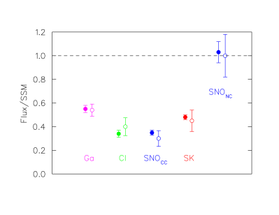
Figure 8: Ratio of solar neutrino flux to SSM (without neutrino oscillations) for various experiments (see text). Filled circles are experimental data (with experimental uncertainties only) and open circles are theoretical expectations based on SSM with best fit parameters to KamLAND and solar-$\nu$ data (uncertainties from SSM and oscillation fit combined). All charged current experiments show a substantial deficit and all are in excellent agreement with the expected values.

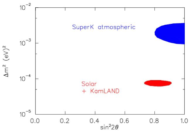
Figure 9: Allowed regions of parameter space (90% C.L.) determined by atmospheric neutrino measurements [62] ($2\leftrightarrow 3$ mixing) and by solar-$\nu$ and reactor-$\bar{\nu}$ measurements [72] ($1\leftrightarrow 2$ mixing).

Table 1: Neutrino Oscillation Parameters Determined From Various Experiments (2003)

Parameter	Value $\pm 1\sigma$	Reference	Comment
$\Delta m_{12}^{2}$	$7.1^{+1.2}_{-0.6}\times 10^{-5}$ eV2	[72]
$\theta_{12}$	${32.5^{\circ+2.4}_{-2.3}}$	[72]	For $\theta_{13}=0$
$\Delta m_{32}^{2}$	$2.0^{+0.6}_{-0.4}\times 10^{-3}$ eV2	[62]
$\sin^{2}2\theta_{23}$	$>0.94$	[62]	For $\theta_{13}=0$
$\sin^{2}2\theta_{13}$	$<0.11$	[64]	For $\Delta m^{2}_{atm}=2\times 10^{-3}$ eV2

3.1.4 LSND

There is one other experiment that claims to observe neutrino oscillations: the Liquid Scintillator Neutrino Detector (LSND) [76] at Los Alamos. In this experiment, the neutrino source was the beam dump of an intense 800 MeV proton beam where a large number of charged pions were created and stopped. Since the $\pi^{-}$ capture on nuclei with very high probability, essentially only the $\pi^{+}$ decay, producing $\nu_{\mu}$ and then $\bar{\nu}_{\mu}$ and $\nu_{e}$ (from $\mu^{+}$ decay). These neutrinos all have very well defined energy spectra (from decays of particles at rest) and note that there are no $\bar{\nu}_{e}$ produced in this process. The 160 ton detector is then used to search for $\bar{\nu}_{e}$ events via inverse beta decay on protons at a distance of 30 m from the neutrino source. The experiment detected an excess of $87.9\pm 22.4\pm 6.0$ events corresponding to an oscillation probability of $0.264\pm 0.067\pm 0.45$%. (Note that such an appearance experiment affords access to very small mixing parameters.) The observed spectrum of events is shown in Fig. 10. Other experiments, especially the KARMEN accelerator experiment [77] and the Bugey reactor experiment [78], rule out much of the allowed region of parameter space but there is a small region remaining at 90% confidence in the mass range $0.2<\Delta m^{2}<10$ eV², indicating a minimum mass of $m_{\nu}>0.4$ eV (see Fig. 12). It is also significant that the KARMEN experiment studied a shorter baseline, which seems to rule out the possibility that the $\bar{\nu}_{e}$ are produced at the source.

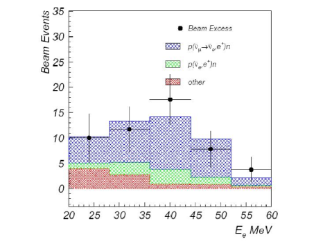
Figure 10: Observed spectrum of positron energy from beam-induced events in the LSND experiment [76]. The black dots are the experimental data, the lower histogram is the estimate of various backgrounds, the middle histogram includes the estimated $\bar{\nu}_{e}$ contamination from the source, and the top histogram includes the neutrino oscillation hypothesis.

Given the well established values of $\Delta m^{2}$ in Table 1, it is not possible to form a third value of $\Delta m^{2}$ consistent with the LSND data (note that $\Delta m_{12}^{2}+\Delta m_{23}^{2}+\Delta m_{31}^{2}=0$). So one would need to either break CPT invariance (allowing $m_{\nu}\neq m_{\bar{\nu}}$), or invoke additional “sterile” neutrinos that do not have the normal weak interactions. In addition, the LSND range of $\Delta m^{2}$ is marginally at variance with recent studies of the cosmic microwave background (see below). Therefore, it is of great importance to attempt to obtain independent verification of this result (see 4.1 below).

3.2 Direct Mass Measurements

Beta decays with low endpoints, in particular tritium $(Q=18.6$ keV), have been used for a long time in attempts to measure or constrain neutrino mass. (¹⁸⁷Re with $Q=2.5$ keV has been also explored recently [79], but the sensitivity is still only 21.7 eV, a factor of about ten worse than for tritium.)

There are several difficulties one has to overcome to reach sensitivities to small neutrino masses in the study of the electron spectrum of $\beta$ decay. Obviously, the mass sensitivity can be only as good as the energy resolution of the electron spectrometer. Also, since by definition the energy spectrum vanishes at the endpoint, the fraction of events in the interval $\Delta E$ near the $Q=E_{0}-m_{e}$ kinetic energy endpoint decreases rapidly, as $(\Delta E/Q)^{3}$. Finally, since the decaying system is a molecule or at best an atom, one has to take into account the possibility that the sudden change of the nuclear charge causes excitations or ionization of the electron cloud, i.e., the presence of multiple endpoints.

Although there are as yet no positive results from direct neutrino mass measurements, these efforts have made (and continue to make) substantial progress (see Fig. 11). Curiously, many past experiments have been apparently plagued by systematic effects that tended to mimic a negative $m_{\bar{\nu}_{e}}^{{\rm(eff)}\ 2}$. As the experiments were improved, it seems that these problems have been largely overcome. Two recent tritium $\beta$ decay experiments have reached impressive results [80, 81] quoting 95% upper limits for the effective mass parameter $m_{\bar{\nu}_{e}}^{{\rm(eff)}}=\sqrt{\sum_{i}|U_{ei}|^{2}m_{i}^{2}}$ of 2.5 eV and 2.8 eV. However, these values are now at the level where atomic and chemical effects on the phase space distributions are significant, and it seems that some of these experiments [81] still occasionally observe anomalous structures near the endpoint. This will likely be a substantial challenge for future measurements of this type.

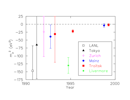
Figure 11: Results of measurements of $m_{\bar{\nu}_{e}}^{2{\rm(eff)}}$ from tritium $\beta$-decay experiments since 1990 [20], showing the steady improvement in the achieved precision.

Constraints from direct mass measurements also exist on $m_{\nu_{\mu}}$ and $m_{\nu_{\tau}}$, but these are much larger (see Section 2.7 for explanation). Given reasonable assumptions, it seems that the oscillation results discussed above and the constraints from tritium decay would imply that the mass values are far below the direct measurements for $\nu_{\mu}$ and $\nu_{\tau}$ so we do not dicuss them in detail here.

3.3 Double Beta Decay

Over the last decade, the methodology for double beta decay experiments has markedly improved. Larger volumes of high-purity enriched materials are being utilized, and careful selection of materials along with deep-underground siting have lowered backgrounds and increased sensitivity. The most sensitive experiments use the isotopes ⁷⁶Ge, ¹⁰⁰Mo, ¹¹⁶Cd, ¹³⁰Te, and ¹³⁶Xe. For ⁷⁶Ge, the lifetime limit has reached an impressive value exceeding $10^{25}$ years. (The experimental results are listed in [20], for the latest review of the field, see [12].) The conversion of the observed lifetime limits to effective neutrino mass values requires use of calculated nuclear matrix elements, and there is some uncertainty associated with them. Nevertheless, the experimental lifetime limits have been interpreted to yield effective mass limits of typically a few eV and in ⁷⁶Ge of 0.3-1.0 eV. One recent report [82], analyzing the ⁷⁶Ge data from the Moscow-Heidelberg experiment, claims to observe a positive signal corresponding to the effective mass $\langle m_{\beta\beta}\rangle=0.39^{+0.17}_{-0.28}$ eV. That report has been followed by a lively discussion [83, 84, 85, 86]. If this finding were to be confirmed then it would be a major advance in our knowledge of neutrino properties, and in particular it would not only prove that neutrinos are Majorana particles, but it would also strongly indicate that neutrinos follow a degenerate mass pattern, where $\Delta m^{2}/m^{2}\ll 1$.

3.4 Cosmological Constraints

In the early universe, when the temperature was $T>1$ MeV, the high density of particles allowed weak interactions to occur prolifically leading to a substantial density of neutrinos. As the universe cooled to $T<1$ MeV, these reactions became much slower than the expansion rate and the neutrinos decoupled from the remaining ionized plasma and radiation (photons). Much later ($\sim 100,000$ years), the universe cooled enough that atoms formed and the radiation decoupled from the matter. The cosmic microwave background (CMB) is the further cooled (through expansion) relic of this period, and contains information on the distribution of matter at that time in the history of the universe. The presently observed distribution of matter (through high resolution galaxy surveys) and distribution of radiation (CMB) would both be affected by the presence of massive neutrinos in the early universe. Although the power spectra of the CMB and the density fluctuations are both sensitive to massive neutrinos, a combined analysis of both observables is especially effective in addressing the existence of massive neutrinos [17, 87]. Thus comparison of the power spectrum of CMB with the observed distribution of galaxies can provide information on the sum (over all flavors) of light neutrino masses. An analysis of the recent WMAP data [88] yields the result $\sum_{f}m_{\nu_{f}}<0.7$ eV (95% confidence). It is interesting to note that this significantly constrains the remaining region of parameter space allowed by LSND. (In addition, interpretation of the LSND result in light of cosmological constraints requires careful consideration of issues related to the behavior (e.g. thermalization) of sterile neutrinos in the early universe. [89]) However, it has been argued that the obtained limit also relies upon input from Lyman-$\alpha$ forest measurements, and that a somewhat less restrictive limit should be quoted [90, 91] Other recent work [92] also obtains a less restrictive limit without the use of strong prior on galaxy bias.

4 Near-term Future

The recent discoveries and revolutionary breakthroughs in the study of neutrino properties have motivated a new generation of experimental efforts aimed at resolving the remaining issues and establishing new launching points for future explorations. These near-term plans and proposals are, for the most part, initiatives that advance the themes we have emphasized above. Neutrino oscillation studies are planned to address the LSND result, higher precision measurements of $\theta_{23}$ and $\Delta m_{23}^{2}$, and determination of $\theta_{13}$. Direct mass measurements are aimed at reducing (or discovering) the absolute value of neutrino masses and establishing the hierarchical nature of the neutrino mass spectrum. And future experiments in double beta decay hope to demonstrate the Majorana nature of neutrinos and constrain (or discover) the mass scale. Finally, the ever increasing precision of cosmological constraints from measurements of the cosmic micowave background promise to provide tighter limits on neutrino masses.

4.1 MiniBooNE

A major near-term priority for the field is to resolve the issue of the validity of the results of the LSND experiment. To this end, the Mini-Boone experiment [93] has been built at FermiLab with the main goal to explore the same region of parameter space with higher sensitivity. This experiment uses a new 0.5-1.5 GeV high-intensity neutrino source and a 800 ton mineral oil-based Čerenkov detector located at 500 m from the source to search for the oscillation modes $\nu_{\mu}\rightarrow\nu_{e}$ and at a later stage $\bar{\nu}_{\mu}\rightarrow\bar{\nu}_{e}$. The projected sensitivity for 2 years running at full beam intensity in each mode is shown in Fig. 12. This experiment has the potential to test the validity of the LSND results with high sensitivity and to explore the possible role of $CPT$ violation by studying both $\nu_{e}$ and $\bar{\nu}_{e}$ appearance. If an effect is seen the collaboration plans to mount another detector at further distance for additional studies. The initial run with the $\nu_{\mu}$ beam began in the Fall of 2002 and first results on oscillations are expected in 2005.

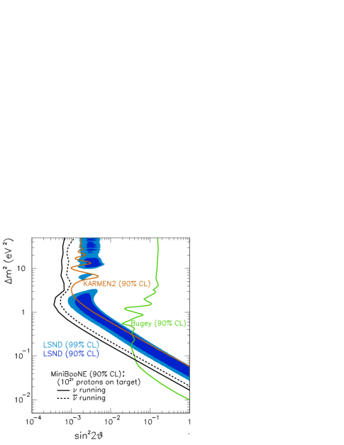
Figure 12: Projected sensitivity [93] of the MiniBooNE experiment compared with LSND and other previous experiments.

4.2 Determination of $\Delta m_{32}^{2}$ and $\theta_{23}$

The phenomenon of neutrino oscillation observed by Super-Kamiokande in the atmospheric neutrino experiment requires further study to precisely determine the mixing parameters $\Delta m_{32}^{2}$ and $\theta_{23}$. There are two long baseline accelerator experiments with prospects for results in the near term: K2K in Japan and MINOS in the US.

The K2K experiment utilizes the 12 GeV proton beam at KEK to produce a $\nu_{\mu}$ beam with average energy 1.3 GeV which is directed at the Super-Kamiokande detector a distance of 250 km [94]. Use of GPS receivers enables clean selection of events with the proper time relative to the beam spill. Careful monitoring of the muons in the $\pi^{+}$-decay region ensures proper aiming of the beam over the long baseline to the detector. In addition, a combination of detectors located 300 m downstream of the $\pi^{+}$ production target is used to measure the flux and energy spectrum of the $\nu_{\mu}$ beam. During the first data run in 1999-2001, the experiment detected 56 fully-contained $\nu_{\mu}$ events, compared to the expected $80.1^{+6.2}_{-5.4}$ events without neutrino oscillations. Thus, so far the K2K experiment appears to confirm the oscillation interpetation of the observed anomaly in the atmospheric neutrino distribution with high probability. By combining the observed energy spectrum and the reduced event rate, the allowed regions shown in Fig. 13 are obtained. The experimental plan is to continue running and roughly double this data sample.

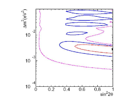
Figure 13: Allowed regions from analysis of the first results from the K2K [94] experiment, representing about 1/2 of the expected total future luminosity. Dashed, solid and dot-dashed lines are 68.4%, 90% and 99% C.L. contours, respectively. The best fit point is indicated by the star.

The MINOS experiment uses the Main Injector proton beam at Fermilab to produce a $\nu_{\mu}$ beam in the energy range 3-18 GeV directed at a large detector located in the Soudan mine at a distance of 735 km [95]. The lowest energy neutrino beam will be optimal for studying the region of $\Delta m_{32}^{2}\simeq 2.0\times 10^{-3}$ eV². This experiment also uses a near detector (1 kton) in addition to the far detector (5.4 kton). The large far detector consists of 486 layers of alternating steel plates with finely (4 cm) segmented plastic scintillator planes. The steel is magnetized by the return flux of a coil located on the detector axis, which enables measurement of muon momentum. With 10 kton-years of exposure at full luminosity, the MINOS experiment should easily confirm the $\nu_{\mu}$ disappearance observed with atmospheric neutrinos and determine the mass parameter $\Delta m_{32}^{2}$ to about 10%. By searching for $\nu_{e}$ appearance the MINOS experiment will be sensitive to $\theta_{13}$ in the region $\sin^{2}\theta_{13}>0.15$ over the presently allowed range of $\Delta m_{32}^{2}$, a factor of $\sim 2$ lower than the CHOOZ limit. The far detector is complete and operating. It is expected that the MINOS experiment will receive the neutrino beam and start operation in 2005.

There is also a long baseline facility from CERN to the Gran Sasso Laboratory ($L\simeq 730$ km). This is a higher energy beam ($\bar{E}_{\nu}\simeq 17$ GeV), suitable for production of $\tau$’s associated with $\nu_{\mu}\rightarrow\nu_{\tau}$ oscillations. There will be two detectors at Gran Sasso for this study: OPERA and ICARUS [96]. The OPERA experiment will employ photographic emulsion to identify the ‘kinks’ associated with the short (few $\mu$m) $\tau$ decays. The ICARUS experiment utilizes a liquid argon time projection chamber to kinematically reconstruct the $\tau$ leptons. Both experiments expect 1-5 events per year to firmly establish this oscillation mode, and will begin operation in 2006. Future experiments providing precision measurements of the corresponding parameters are highly desirable.

4.3 Studies of $\theta_{13}$, Neutrino Mass Hierarchy, and $CP$ Violation

The role of mixing between the first and third generation neutrino mass eigenstates is pivotal in terms of the phenomenological consequences. The possibility of $CP$ violation and implications for leptogenesis scenarios in generating the matter-antimatter asymmetry in the universe require mixing between these two states. Therefore, establishment of non-vanishing mixing (i.e., $\theta_{13}\neq 0$) is of paramount importance and substantial experimental efforts are planned to address this issue.

4.3.1 High-precision Reactor Neutrino Experiments

When completed, the KamLAND experiment will significantly reduce the allowed region for $\Delta m_{12}^{2}$ and $\tan^{2}\theta_{12}$ relative to the present results shown in Fig. 7. The next major goal for the reactor neutrino program will be to attempt a measurement of $\sin^{2}\theta_{13}$. As can be seen from Eq. (23) and as discussed in section 2 above, such experiments have the potential to determine $\theta_{13}$ without ambiguity from $CP$ violation or matter effects. The strategy is to capitalize on the success of CHOOZ and KamLAND to build a new experiment at the $1.5-2$ km distance now indicated by the Super-Kamiokande atmospheric neutrino results. Obtaining the necessary statistical precision on this challenging disappearance experiment will require large reactor power ($>5$ GWth) and large detector size (probably $\sim 100$ ton). Systematic errors must be carefully controlled through reduced background and utilization of a two detector scheme (probably in a configuration with a near detector at a close $\sim 100-200$ m distance from the reactor(s) in addition to the far detector at $\sim 2$ km). Backgrounds must be controlled through sufficient depth underground ($>300$ m to reduce cosmic ray induced spallation products), careful choice of detector materials, and passive shielding (e.g., buffer of water or mineral oil) to reduce events due to radioactive decays in the surrounding rock and other material. Comparison of the rates and observed spectral shapes in the two detectors will reduce the sensitivity to reactor source uncertainties and provide substantial improvements in the sensitivity to reactor antineutrino disappearance in this region. With the anticipated statistical and systematic uncertainties held to a total of order 1%, the sensitivity will reach about $\sin^{2}2\theta_{13}\simeq 0.01-0.02$ at the optimal value of $\Delta m^{2}\sim 2.0\times 10^{-3}$ eV² derived from the Super-Kamiokande results. Significant efforts are presently underway to optimize the experimental design and select appropriate sites for this future experiment. [97, 98, 99]

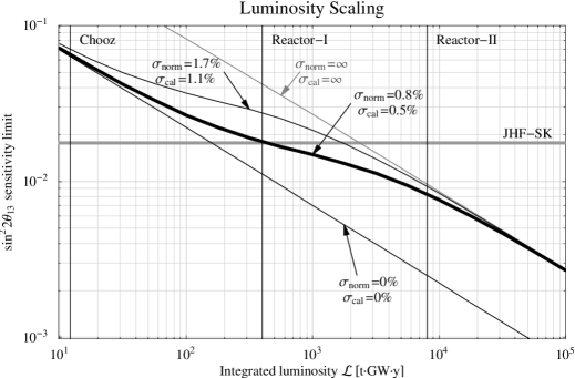
Figure 14: Projected sensitivity (90% C.L.) of future reactor neutrino experiements to $\theta_{13}$ as a function of integrated luminosity [97]. The authors assumed $\Delta m_{31}^{2}=3.0\times 10^{-3}$ eV² and studied scenarios with various systematic errors for flux normalization ($\sigma_{\rm norm}$) and energy calibration ($\sigma_{\rm cal}$). The JHF-SK line is the projected sensitivity of the future JPARC-SK experiment (see 4.3.2 below), Reactor-I scenario is 400 GW-ton-years, and Reactor-II scenario is 8000 GW-ton-years.

Fig. 14 shows the results of a general study of the potential of such experiments [97]. With reasonable systematic errors ($<1\%$) for normalization and energy calibration it is apparent that about 400 GW-ton-years of luminosity would provide a determination of $\sin^{2}2\theta_{13}$ with sensitivity better than 0.02. In addition, the figure shows interesting behavior at higher luminosity ($\sim 8000$ GW-ton-years) where the sensitivity improves as $1/\sqrt{\mathcal{L}}$ due to the high statistical precision in determination of the relative spectral shapes at the near and far detectors. (The curve with $\sigma_{norm}$ and $\sigma_{cal}=\infty$ describes the situation where the absolute efficiency and energy calibration of the near and far detectors becomes irrelevant, but the relative efficiencies and energy calibrations must be still tightly controlled.) Although the realization of siting KamLAND-scale detectors near large power reactor plants would be very challenging, the increased sensitivity to $\sin^{2}2\theta_{13}$ at such high luminosities would be of great interest.

4.3.2 Long Baseline Accelerator Experiments

While the reactor neutrino studies at $\sim 2$ km have the potential to establish a non-vanishing mixing and a numerical value for $\theta_{13}$, further studies related to the neutrino mass hierarchy and the role of $CP$ violation will require mounting new long baseline accelerator experiments (see Sections 2.4 and 2.5). The potential for studying these phenomena is evident in Eq. (53) and illustrated in Fig. 15 where one can see the effects of varying the CP-violation parameters and changing the mass hierarchy. There is a great deal of activity in this subject at the moment, and a variety of proposed scenarios are under discussion.

The main features of the next generation long baseline accelerator experiments include:

• ability to detect the $\nu_{\mu}\rightarrow\nu_{e}$ process as the major goal,

• $L/E_{\nu}\sim 500$ km/GeV to optimize the oscillation probability for $\Delta m_{23}^{2}\sim 3\times 10^{-3}$ eV²,

• propagation of the $\nu$ beam through the earth, resulting in sensitivity to matter effects,

• possibility to vary $L/E_{\nu}$ by adjusting the focusing horn, target position, and/or detector location,

• possibility to switch to $\bar{\nu}_{\mu}$.

A significant new concept, the “off-axis” neutrino beam [100] (combined with a substantial increase in the neutrino flux and often referred to as a “super-beam”), appears to be a very attractive option for these experiments. By positioning the detector off the symmetry axis (at a so-called “magic” angle), the neutrino energy becomes stationary with respect to the pion energy and an essentially monoenergetic neutrino beam is obtained. Although generally some loss of flux results from the off-axis geometry, the advantages include a tuneable narrow-band beam with significant suppression of the higher energy tail and very low $\nu_{e}$ contamination. Thus one can selectively scan a range of $\Delta m^{2}$ to measure the dependence of the oscillation probability with reduced background rates (both due to the low $\nu_{e}$ flux and the suppressed $\pi^{0}$ production from higher energy neutral current events). This method has been adopted for both the JPARC-SK experiment and the Fermilab NUMI proposal.

The JPARC facility [101] will be a high luminosity (0.77 MW beam power) 50 GeV proton synchrotron with neutrino production facility aimed about $2^{\circ}$ off-axis from the Super-Kamiokande detector ($L\simeq 295$ km). The resulting low-energy ($\sim 0.7$ GeV) neutrino beam at the Super-K site will enable sensitivity to $\sin^{2}2\theta_{13}\sim 6\times 10^{-3}$ after about 5 years running. It is expected that the experiment would start in 2008, and upgrades involving siting a 1Mt detector and increased beam intensity are envisioned for the future, with potential sensitivity to $\sin^{2}2\theta_{13}<1.5\times 10^{-3}$ and $CP$-violating phase $\delta\sim\pm 20^{\circ}$.

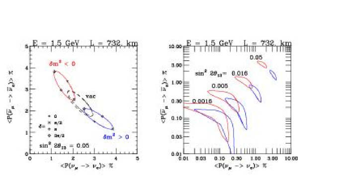
Figure 15: Oscillation probabilities for neutrino and antineutrino oscillations [103] for the NUMI experiment parameters [102]. The different loops correspond to various values of $\sin^{2}\theta_{13}$ and normal and inverted hierarchy. The variation of the CP-violating phase $\delta$ traces the loops.

The “Off-axis NUMI” proposal [102] is to site a new detector either near Soudan at $L\sim 715$ km or at a further site in Canada at $L\sim 950$ km, at an angle of about 14 mrad with respect to the beam axis. The neutrino beam energy will be about 2 GeV, and with a 20 kt detector (still under development) the sensitivity would be comparable to the JPARC-SK experiment, but the higher energy of this neutrino beam improves the sensitivity to the sign of $\Delta m_{23}^{2}$ (i.e., normal vs. inverted hierarchy).

There is also discussion of a plan [104] to upgrade the AGS at Brookhaven to higher beam power and construct a neutrino beam aimed at the proposed new underground laboratory (NUSL) in Lead, South Dakota or some other underground location at a similar distance. This would afford the opportunity to perform measurements with a large ($~{}0.5$ Mt) detector at a distance of $L\sim 2500$ km, as well as with a closer off-axis detector ($L\sim 400$ km). Such measurements could convincingly demonstrate the oscillatory behavior of the flavor transformations with high statistics.

4.4 Future Direct Mass Measurements

A new experiment to study the tritium $\beta$-endpoint spectrum, KATRIN, is under development [105]. In order to improve the sensitivity to neutrino masses by an order of magnitude it is necessary to both reduce the energy resolution of the spectrometer (to $\sim 1$ eV) and increase the tritium source strength (to improve statistical precision). The basic strategy for achieving these goals is to scale up the previous spectrometer design used in the successful Mainz and Troitsk experiments to a larger physical size, as shown in Fig. 16. The larger size enables a higher ratio of magnetic fields $B_{\rm max}/B_{\rm min}$ to improve the energy resolution and a larger source acceptance to increase the luminosity. The previous spectrometers were 1-1.5 m in diameter and the new KATRIN design is 7 m diameter. Both a windowless gaseous tritium source and a condensed source will be utilized to enable studies of potential systematic effects associated with the different source methods. The goal for the tritium source is a column density of $5\times 10^{17}$ molecules/cm² and a maximum accepted take-off angle of $\theta_{\rm max}=51^{\circ}$. These parameters will enable sensitivity to neutrino masses in the sub-eV range, hopefully down to $\sim 0.35$ eV.

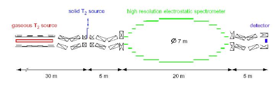
Figure 16: Conceptual design for the KATRIN experiment for higher-precision measurements of the neutrino mass using the endpoint of the tritium $\beta$-decay spectrum.

4.5 Plans for Double Beta Decay

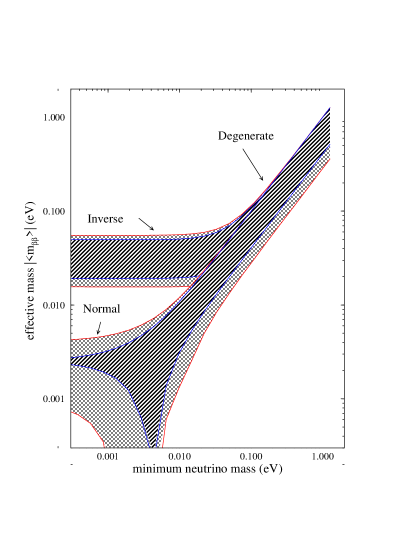
Figure 17: Dependence of the effective Majorana mass $\langle m_{\beta\beta}\rangle$ derived from the rate of neutrinoless double beta decay ($1/T_{1/2}^{0\nu}\sim\langle m_{\beta\beta}\rangle^{2}$) on the absolute mass of the lightest neutrino. The stripes region indicates the range related to the unknown Majorana phases, while the cross hatched region is covered if one $\sigma$ errors on the oscillation parameters are also included. The arrows indicate the three possible neutrino mass patterns or “hierarchies”.

In contrast to the future direct neutrino mass measurements described above in 4.4, the next generation of double beta decay searches is poised to address the mass scale indicated by the atmospheric $\nu$ measurements of Super-Kamiokande ($\Delta m_{32}^{2}\simeq 2.0\times 10^{-3}$ eV²) and perhaps even approach the scale of the solar $\nu$ solution ($\Delta m_{12}^{2}\simeq 1\times 10^{-4}$ eV²). For the case of normal hierarchy ($m_{1}\sim m_{2}\ll m_{3}$), there is a rather firm prediction for the effective mass relevant to $\beta\beta$ decay:

$$m_{\beta\beta}^{2}\simeq{\rm Max}\left[|U_{e3}^{2}m_{3}|^{2},~{}|\sin\theta_{12}^{2}m_{2}|^{2}\right]\sim 10^{-5}{\rm eV}^{2}~{}.$$ (68)

This mass scale of less than 3 meV is difficult to address in the near future, but if nature actually chooses the inverted hierarchy ($m_{1}\sim m_{2}\gg m_{3}$), then the $\beta\beta$ prediction becomes

$$m_{\beta\beta}^{2}\simeq|U_{e1}^{2}m_{1}|^{2}+|U_{e2}^{2}m_{2}|^{2}\sim m_{1}^{2}\sim 10^{-3}{\rm eV}^{2},$$ (69)

corresponding to an effective mass scale of about 30 meV. For the degenerate neutrino mass pattern ($m_{1}\sim m_{2}\sim m_{3}\gg\sqrt{\Delta m_{32}^{2}}$) the effective mass is larger than $\sim$ 50 meV, constrained from above by the mass limit from the tritium beta decay.

The relation between the effective mass in $\beta\beta$ decay and the mass of the lightest neutrino, evaluated for the solar $\nu$ solution (see Table 1), is shown in Fig. 17.

Table 2: Proposed or suggested future $0\nu\beta\beta$ experiments separated into two groups based on the magnitude of the proposed isotope mass^a.

			Sensitivity to	range of
Experiment	Source	Detector Description	$T_{1/2}^{0\nu}$ (y)	$\langle m_{\beta\beta}\rangle$ (meV)
COBRA[106]	130Te	10 kg CdTe semicond.	$1\times 10^{24}$	700-2400
DCBA[107]	150Nd	20 kg enrNd layers	$2\times 10^{25}$	35-50
		between tracking chambers
NEMO 3[108]	100Mo	10 kg of $0\nu\beta\beta$ isotopes	$4\times 10^{24}$	270-1000
		(7 kg Mo) with tracking
CAMEO[109]	116Cd	1 t CdWO4 crystals	$>10^{26}$	$>$ (70-220)
		in liq. scint.
CANDLES[110]	48Ca	several tons of CaF2	$1\times 10^{26}$	160-300
		crystals in liq. scint.
CUORE[111]	130Te	750 kg TeO2 bolom.	$2\times 10^{26}$	50-170
EXO[112]	136Xe	1 t enrXe TPC	$8\times 10^{26}$	50-120
GEM[113]	76Ge	1 t enrGe diodes	$7\times 10^{27}$	15-50
		in liq. nitrogen
GENIUS[114]	76Ge	1 t 86% enrGe diodes	$1\times 10^{28}$	13-42
		in liq. nitrogen
GSO[115, 116]	160Gd	2 t Gd2SiO5:Ce crystal	$2\times 10^{26}$	65
		scint. in liq. scint.
Majorana[117]	76Ge	0.5 t 86% segmented	$3\times 10^{27}$	24-77
		enrGe diodes
MOON[118]	100Mo	34 t natMo sheets	$1\times 10^{27}$	17-60
		between plastic scint.
Xe[119]	136Xe	1.56 t of enrXe	$5\times 10^{26}$	60-150
		in liq. scint.
XMASS[120]	136Xe	10 t of liq. Xe	$3\times 10^{26}$	80-200

^a Adopted from [12]. The $T_{1/2}^{0\nu}$ sensitivities are those estimated by the collaborators but scaled for 5 years of data taking. These anticipated limits should be used with caution since they are based on assumptions about backgrounds for experiments that do not yet exist. Since some proposals are more conservative than others in their background estimates, one should refrain from using this table to contrast the experiments. The range of the effective masses $\langle m_{\beta\beta}\rangle$ reflects the range of the calculated nuclear matrix elements (see Table 2 of Ref. [12]). Again, caution should be used since for some nuclei, in particular the deformed ¹⁵⁰Nd and ¹⁶⁰Gd, only few calculations exist and the approximations are even more severe than in the other cases.

Present estimates of the nuclear matrix elements [12] involved in the $\beta\beta$ process indicate that, with of order several tons of enriched material, experiments could reach this interesting mass range.

There are many proposed experiments to address this issue in the near future. Most are still in the development stage, and of course the issue of backgrounds is critical in every case. Since the source mass is $\sim$ 100 times larger than in the present experiments, the background per unit mass must be correspondingly smaller. Different proposals approach this issue differently, and in all cases substantial R&D is required. Nevertheless, it appears that several experiments will be mounted during the next decade with the goal of studying $0\nu\beta\beta$ with sensitivity below 30 meV. The Table 2 lists the proposed experiments we are aware of, together with the claimed sensitivity to the $0\nu\beta\beta$ halflife, and its crude translation into the sensitivity to the Majorana mass.

Among the listed experiments, a few relatively small scale searches are actually running (COBRA, NEMO3). Others, particularly the ‘ton size’, will be mounted in stages with prototypes of 50-200 kg approved and funded at the present time for several of them (one, CUORICINO, the prototype of CUORE, with 40 kg of natural Te, is already running in Gran Sasso). Clearly, the final decision as to which of these many ideas will be realized depends on the outcome of these prototype installations. Nevertheless, since they are still $\sim$ 10 times larger than the present experiments, we can expect substantial improvement in sensitivity relatively soon.

4.6 Cosmological Input

In the near-term future, substantial additional information from cosmological observations will become available that will further constrain the sum of light neutrino masses $\sum_{f}m_{\nu_{f}}$ compared to the limits quoted in 3.4. Already in progress is the Sloan Digital Sky Survey (SDSS) [121] that will map over $10^{6}$ galaxy redshifts and provide relative sensitivity in the relevant region of the power spectrum of $\sim 1\%$. When combined with the WMAP CMB data, this should provide sensitivity to $\sum_{f}m_{\nu_{f}}\sim 0.3$ eV [87]. Further in the future, higher precision measurements of the CMB anisotropies are expected from the PLANCK mission (now expected to be launched in 2007) [122]. An estimate of the combined sensitivity ($1\sigma$) of the expected PLANCK data and the SDSS observations to neutrino masses gives the result $\sum_{f}m_{\nu_{f}}\sim 0.06$ eV [123].

5 Longer-term Outlook

It is difficult to envision what direction the study of neutrino mass and oscillations will take in the longer-term. Thus, we can only offer educated guesses.

Some of the future research will, obviously, depend on the results of the near-term future described in the preceding section. Among the results that might force a revision of the experimental program are the MiniBooNE tests of the LSND evidence for the $\bar{\nu}_{\mu}\rightarrow\bar{\nu}_{e}$ oscillations corresponding to $\delta m^{2}>0.2$ eV², and the attempts to determine the mixing angle $\theta_{13}$.

If MiniBooNE confirms the LSND observation, many more experiments will be needed because the nature of the neutrino mixing matrix would be much richer (more than just three active neutrinos or $CPT$ invariance violation) than envisioned so far and summarized in Table 1. Also, if it turns out that the mixing angle $\theta_{13}$ is relatively large, perhaps close to the present upper limit, the study of the possible $CP$ invariance violation in the neutrino sector will become considerably easier and will proceed faster than if $\theta_{13}$ is very small.

In addition, neutrino astrophysics will undoubtedly advance. Further studies of the solar neutrino spectrum will be conducted, and in particular the low energy part, the flux of the ⁷Be and $pp$ neutrinos, will be likely determined in live counting experiments. These measurements will be valuable not only for the further refinement of the determination of the oscillation parameters $\Delta m_{12}^{2}$ and $\theta_{12}$, but also for better understanding of solar energy production.

Moreover, with several experiments on-line, we can hope that in the near future the next galactic core collapse supernova will be observed by a variety of neutrino detectors. If that happens, the observation of SN1987A [124] which launched this field of neutrino astrophysics, will be exceeded many times, and all components of the supernova neutrino spectrum will be observed. Again, such observations would not only advance our knowledge of neutrino physics, but will offer a unique insight in the physics of the stellar core collapse.

We also anticipate that during the next decade other applications of neutrino physics will become reality. For example, the observation of ‘geoneutrinos’, i.e. the $\bar{\nu}_{e}$ emitted by the decay of radioactive U and Th series in the Earth crust [75, 125, 126] would enable determination of the corresponding radiogenic heat generation and provide an important contribution to geophysics. Another application is the measurement of the relic supernova flux: the diffuse flux resulting from past supernovae in the surrounding space, roughly up to redshift $z=1$. By measuring this flux one can determine the average supernova rate over a substantial part of the visible universe (for an estimate of the rate see e.g. [127]).

At present, neutrino telescopes have not yet seen the TeV and higher energy neutrinos which likely accompany the production of cosmic rays with such energies. This might change in near future when the relatively small underground detectors are supplemented by much larger ones in open water or ice. Observation of the direction of high energy neutrinos would considerably advance the study of the origin of high energy cosmic rays [128]. It will also make it possible to search for neutrinos from annihilation of the so far hypothetical dark matter particles (WIMPs). It is beyond the scope of this review to describe the projects being built or proposed (see [129] for a recent review).

Naturally, the whole field of particle physics will advance at the same time. With the launch of LHC one can imagine that the existence of the Higgs boson will be experimentally confirmed, and its properties will be, at least crudely, determined. One can also hope that the quest for the understanding of the two main paradigm of present day physics, the nature of the ‘dark matter’ and ‘dark energy’, responsible for most of the energy density of the Universe, will be advanced.

These more general areas of particle physics could be, in fact, intimately related to the quest for neutrino mass and oscillations. Taking the see-saw formula ${\mathcal{M}_{L}=\mathcal{M}_{D}}^{2}/{\mathcal{M}_{H}}$, and using for ${\mathcal{M}_{L}}$ the neutrino mass scale $\sim$10 meV and for ${\mathcal{M}_{D}}$ the electroweak symmetry breaking mass scale $\sim$ 100 GeV, we arrive at ${\mathcal{M}_{L}}\sim 10^{15}$ GeV, i.e. close to the GUT unification mass scale. If that relation could be firmed up, we will arrive at another determination of that important mass scale. The relation of the neutrino mass scale to the ‘dark energy’ is based on the, perhaps accidental, numerical coincidence. Remembering that the energy density of the ‘dark energy’ is about $0.7\Omega_{c}\sim 3.5\times 10^{3}$ eV/cm³ and rewriting it in the ‘natural units’ as $\epsilon^{4}/(\hbar c)^{3}$ we arrive at the dark energy mass scale $\epsilon\sim$ 2 meV, close to the neutrino mass scale, and unlike any other mass scale in particle physics. (For recent attempts to relate these two mass scales see e.g., [130].)

Future large scale projects to generate powerful new beams of neutrinos are already envisioned. To explore the possibility of $CP$ violation in the lepton sector one would like to have a well-understood and collimated neutrino beam of a well defined flavor and energy spectrum. Such a beam could be aimed at a distant large detector. Recently it has been pointed out that technology exists to construct pure $\nu_{e}$ and $\bar{\nu}_{e}$ beams of the required properties. Accelerating radioactive ions, ⁶He ($E_{0}=3.5$ MeV, $T_{1/2}=0.8$s, produces $\bar{\nu}_{e}$) or ¹⁸Ne ($E_{0}=4.45$ MeV, $T_{1/2}=0.8$s, produces $\nu_{e}$) to $\gamma\simeq 100$, would produce beams of precisely known energy profile extending to $2\gamma E_{0}$, and collimated to $1/\gamma$. The oscillation signature in the far away detector would be the appearance of $\mu^{+}$ or $\mu^{-}$ [131]. It is expected that $O(10^{18})$ decays per year can be achieved.

The beams of $\nu_{\mu}$ and $\bar{\nu}_{\mu}$ as well as $\nu_{e}$ and $\bar{\nu}_{e}$ neutrinos could be obtained in a neutrino factory where accelerated muons are stored in a ring with long straight sections. Such a beam will produce neutrino beams with equal mixtures of $\bar{\nu}_{\mu}$ and $\nu_{e}$ if $\mu^{+}$ are stored, and $\nu_{\mu}$ with $\bar{\nu}_{e}$ if $\mu^{-}$ are stored. It is expected that neutrino factories could provide $O(10^{20})$ useful muon decays per year. Neutrino factories would thus provide beams with small systematic uncertainties in the beam flux and spectrum. $CP$ violation, and determination of $\sin^{2}2\theta_{13}$ even if it is as small as $10^{-4}-10^{-5}$ can be achieved with such beams and baselines of several thousand km [132].

One indication of the importance of the study of neutrinos is the recent report “Facilities for the Future Science, A Twenty-Year Outlook” (see http://www.sc.doe.gov/). It lists two projects, among the 28 listed in all fields supported by the US Department of Energy, relevant to the present topic, the study of double beta decay in underground detectors treated among the mid-term projects and Super Neutrino Beam treated as a far-term project.

Clearly there are high expectations in the community of particle physicists that experiments with neutrinos will continue to provide new insights and substantial progress in the coming decades. Construction and operation of the required facilities will be challenging, but the potential rewards are great, and a large and talented community of physicists is poised to embark on this unique and interesting journey.

6 Acknowledgements

We would like to thank Felix Boehm for encouragement and inspiration resulting from his long and pioneering search for neutrino oscillations at nuclear reactors. We thank John Beacom and Gerry Garvey for reading the manuscript and for helpful comments. This work was supported in part by the US DOE Grant DE-FG03-88ER40397.

References

- [1] W. Pauli, letter to a physicist’s gathering at Tubingen, December 4, 1930. Reprinted in Wolfgang Pauli, Collected Scientific Papers, ed. R. Kronig and V. Weisskopf, Vol. 2, p.1313 (Interscience: New York, 1964).
- [2] C. L. Cowan, Jr., F. Reines, F. B. Harrison, H. W. Kruse, and A. D. McGuire, Science 124, 103 (1956); F. Reines and C. L. Cowan, Phys. Rev. 92, 830 (1953).
- [3] M. Gell-Mann, P. Ramond and R. Slansky, in Supergravity, D. Freedman and P. van Nieuwenhuizen eds., North Holland, Amsterdam 1979; T. Yanagida, in Proc. of the Workshop on Unified Theory amd Baryon Number of the Universe, O. Sawada and A. Sugamoto eds., KEK, Japan (1979); R. N. Mohapatra and G. Senjanovic, Phys. Rev. Lett. 44, 912 (1980).
- [4] F. Boehm and P. Vogel, Physics of Massive Neutrinos, 2nd ed., Cambridge Univ. Press, Cambridge 1992.
- [5] B. Kayser, F. Gibrat-debut and F. Perrier, Massive Neutrinos, World Scientific, Singapore 1989.
- [6] R. N. Mohapatra and P. B. Pal, Massive Neutrinos and Physics and Astrophysics 2nd ed. World Scientific, Singapore 1998.
- [7] D. O. Caldwell (ed), Current Aspects of Neutrino Physics, Springer, Heidelberg, 2001.
- [8] J. N. Bahcall, Neutrino Astrophysics, Cambridge Univ. Press, Cambridge 1989.
- [9] K. Winter, Neutrino Physics, 2nd ed. Cambridge Univ. Press, Cambridge 2000.
- [10] G. Raffelt, Stars as Laboratories for Fundamental Physics, University of Chicago Press, Chicago, 1995.
- [11] P. Fisher, B. Kayser and K. S. McFarland, Ann. Rev. Nucl. Part. Sci. 49, 481 (1999).
- [12] S. R. Elliott and P. Vogel, Ann. Rev. Nucl. Part. Sci. 52, 481 (2002).
- [13] V. Barger, D. Marfatia and K. Whisnant, hep-ph/0308123
- [14] M. C, Gonzales-Garcia and Y. Nir, Rev. Mod. Phys. 75, 345 (2003).
- [15] C. Bemporad, G. Gratta and P. Vogel, Rev. Mod. Phys. 74, 297 (2002).
- [16] G. Altarelli and F. Feruglio, Phys. Rep. 320, 295 (1999).
- [17] S. M. Bilenky, C. Giunti, J. A. Grifols, and E. Masso, Phys. Rep. 379, 69 (2003).
- [18] S. F. King, hep-ph/0310204.
- [19] V. Barger et al., Phys. Lett. B566, 8 (2003); R. H Cyburt, B. D. Fields, and K. A. Olive, Phys. Lett. B567, 227 (2003)
- [20] Particle Data Group, “Review of Particle Properties”, Phys. Rev. D66, 010001-381 (2002).
- [21] A. de Gouvêa, B. Kayser, R. N. Mohapatra, Phys.Rev.D 67, 053004 (2003).
- [22] C. Giunti, Phys. Scripta 67, 29 (2003); M. Beuthe, Phys. Rept. 375, 105 (2003).
- [23] B. Pontecorvo, Sov. Phys. JETP 6, 429 (1958).
- [24] B. Pontecorvo, Sov. Phys. JETP 33, 549 (1967).
- [25] Z. Maki, M. Nakagawa and S. Sakata, Prog. Theor. Phys. 28, 870 (1962).
- [26] N. Cabibbo, Phys. Lett. 72B, 333 (1978).
- [27] V. Barger, K. Whisnant, and R. J. N. Phillips, Phys.Rev.Lett. 45, 2084 (1980).
- [28] L. Wolfenstein, Phys. Rev. D 17, 2369 (1978).
- [29] V. Barger, K. Whisnant, S. Pakvasa, and R. J. N. Phillips, Phys. Rev. D 22, 2718 (1980).
- [30] R. R. Lewis, Phys. Rev. D 21, 663 (1980).
- [31] P. Langacker, J. P. Leveillé and J. Sheiman, Phys. Rev. D 27, 1228 (1983).
- [32] A. de Gouvêa, A. Friedland and H. Murayama, Phys. Lett. B490, 125 (2002).
- [33] G. L. Fogli, E. Lisi and D. Montanino, Phys. Rev. D 54 2048 (1996).
- [34] S. P. Mikheyev and A. Yu. Smirnov, Sov. J. Nucl. Phys. 42, 913 (1986); Sov. Phys. JETP 64, 4 (1986); Nuovo Cim. 9C, 17 (1986).
- [35] S. J. Parke, Phys. Rev. Lett. 57, 1275 (1986).
- [36] V. Barger, S. Pakvasa, T. J. Weiler and K. Whisnant, Phys.Rev.Lett. 85, 5055 (2000).
- [37] V. A. Kostelecky and M. Mewes, hep-ph/0309025 and references therein.
- [38] H. Murayama and T. Yanagida, Phys. Lett. B520, 263 (2001).
- [39] G. Barenboim, L. Borissov, J. Lykken and A. Y. Smirnov JHEP 0210, 001 (2002); G. Barenboim, L. Borissov and J. Lykken Phys. Lett. B534, 106 (2002); G. Barenboim, J. F. Beacom, L. Borissov and B. Kayser, Phys. Lett. B537, 227 (2002).
- [40] G. Barenboim, L. Borissov and J. Lykken, hep-ph/0212116.
- [41] H. Murayama, hep-ph/0307127.
- [42] M. C. Gonzalez-Garcia, M. Maltoni and T. Schwetz, Phys. Rev. D68, 053007 (2003).
- [43] M. W. Diwan et al., Phys. Rev. D68, 012002(2003).
- [44] V. Barger, D. Marfatia and K. Whisnant, Phys. Rev. D65, 073023 (2002).
- [45] K. Eguchi et al., hep-ex/0310047
- [46] S. Bilenky and B. Pontecorvo, Lett. Nuovo Cim. 17, 569 (1976).
- [47] P. Langacker and J. Wang, Phys. Rev. D58, 093004 (1998) and references therein.
- [48] J. Schechter and J. Valle, Phys. Rev. D25, 2951 (1982).
- [49] A. Faessler and F. Šimkovic, J. Phys. G24,2139 (1998).
- [50] J. Suhonen and O. Civitarese, Phys. Rep. 300, 123 (1998).
- [51] V. Rodin, A. Faessler, F. Šimkovic and P. Vogel, Phys. Rev. c68, 044302 (2003).
- [52] K. Zuber, hep-ph/0008080.
- [53] K. Arisaka, et al., J. Phys. Soc. Jpn. 54, 3213 (1985); K. S. Hirata, et al., Phys. Rev. D38, 448 (1988).
- [54] R. Bionta, et al., Phys. Rev. Lett. 54, 22 (1985).
- [55] H. Georgi and S. L. Glashow, Phys. Rev. Lett. 32, 438 (1974).
- [56] K.S. Hirata, et al., Phys. Lett. B280, 146 (1992).
- [57] R. A. Becker-Szendy, et al., Phys. Rev. D46, 3720 (1992).
- [58] E. W. Beier, et al., Phys. Lett. B283, 446 (1992).
- [59] W. W. M. Allison et al., Phys. Lett. B391, 491 (1997).
- [60] K. Scholberg, et al., Proceedings of 8th International Workshop on Neutrino Telescopes, Venice, February 23-26 1999 (hep-ex/9905016).
- [61] Y. Fukuda, et al., Phys. Rev. Lett. 81, 1562 (1998).
- [62] K. Nishikawa, Lepton-Photon Conference 2003 (http://conferences.fnal.gov/lp2003/program/S10/).
- [63] M. Ambrosio et al., Phys. Lett. B517, 59 (2001).
- [64] M. Appolonio, et al., Phys. Lett. B466, 415 (1999).
- [65] F. Boehm, et al., Phys. Rev. D64, 112001 (2001).
- [66] John N. Bahcall, M. H. Pinsonneault, and Sarbani Basu, Astrophys. J. 555, 990 (2001).
- [67] John N. Bahcall, Astrophys. J. 467, 475 (1996); John N. Bahcall, Sarbani Basu, and M. H. Pinsonneault, Phys. Lett. B433, 1 (1998).
- [68] B. T. Cleveland, et al., Astrophys. J. 496, 505 (1998).
- [69] J. N. Abdurashitov, et al., Phys. Rev. C60, 055801 (1999); W. Hampel, et al., Phys. Lett. B447, 127 (1999).
- [70] Y. Fukuda, et al., Phys. Rev. Lett. 77, 1683 (1996).
- [71] Y. Fukuda, et al., Phys. Rev. Lett. 81, 1158 (1998); S. Fukuda, et al., Phys. Lett. B539, 179 (2002).
- [72] S. N. Ahmed, et al., nucl-ex/0309004.
- [73] Q. R. Ahmad, et al., Phys. Rev. Lett. 87, 071301 (2001).
- [74] Q. R. Ahmad et al., Phys. Rev. Lett. 89, 011301 (2002).
- [75] K. Eguchi et al., Phys. Rev. Lett. 90, 021802 (2003).
- [76] A. Aguilar et al., Phys. Rev. D64, 112007 (2001).
- [77] B. Armbruster et al., Phys. Rev. D65, 112001 (2002).
- [78] B. Achkar et al., Phys. Lett. B374, 243 (1996).
- [79] C. Amalboldi et al., hep-ex/0302006.
- [80] Ch. Weinheimer et al., Phys. Lett. B460, 219 (1999); Ch. Weinheimer et al., Phys. Lett. B464, 352 (1999).
- [81] V. M. Lobashev et al., Phys. Lett. B460, 227 (1999).
- [82] H. V. Klapdor-Kleingrothaus et al., Mod. Phys. Lett. 16, 2409 (2001).
- [83] C. E. Aalseth et al., Mod. Phys. Lett. 17, 1475 (2002).
- [84] F. Feruglio, A. Strumia and F. Vissani, Nucl. Phys. B637, 345 (2002).
- [85] H. V. Klapdor-Kleingrothaus, A. Dietz and I. Krivosheina, Found.Phys. 32, 1181 (2002).
- [86] A. M. Bakalyarov et al., hep-ph/0309016.
- [87] Wayne Hu, Daniel J. Eisenstein, and Max Tegmark, Phys. Rev. Lett. 80, 5255 (1998
- [88] D. N. Spergel, et al., Astrophys. J. Suppl. 148 175 (2003).
- [89] J. Beacom, private communication.
- [90] O. Elgaroy and O. Lahev, JCAP 0304, 004 (2003); astro-ph/030389.
- [91] S. Hannestead, JCAP 0305, 004 (2003); astro-ph/030376.
- [92] M. Tegmark, et al., astro-ph/0310723.
- [93] A. O. Bazarko, et al., hep-ex/0210020.
- [94] M. H. Ahn, et al., Phys. Rev. Lett. bf 90 041801 (2003).
- [95] M. V. Diwan, hep-ex/0211026.
- [96] F. Arneodo, talk at TAUP2003; http://int.phys.washington.edu/taup2003.
- [97] P. Huber et al., Nucl.Phys. B665 487 (2003).
- [98] F. Suekane, et al., proceedings of 4th Workshop on Neutrino Oscillations and their Origin (NOON2003), Kanazawa, Japan, 10-14 Feb 2003.
- [99] “White Paper on Measuring With a Reactor Experiment”, (http://www.hep.anl.gov/minos/reactor13/white.html).
- [100] D. Beavis et al., BNL AGS proposal E889 (1995).
- [101] “Accelerator Technical Design Report for High-Intensity Proton Accelerator Facility Project”, J-PARCKEK Report 2002-13 (http://hadron.kek.jp/member/onishi/tdr/index.html).
- [102] D. Ayres et al., Letter of Intent P929 to Fermilab, 2002 (http://www-off-axis.fnal.gov/).
- [103] H. Minakata and H. Nunokawa, JHEP 0110, 001 (2001). [hep-ph/0108085]
- [104] D. Beavis et al., Letter of Intent to Brookhaven National Laboratory, 2002 (http://www.neutrino.bnl.gov/).
- [105] A. Osipowicz et al.,, hep-ex/0109033; L. Bornschein for KATRIN collaboration, hep-ex/0309007
- [106] Zuber K, Phys.Lett. B519:1 (2001)
- [107] Ishihara N, et al., Nucl. Instrum. Meth. A443:101 (2000)
- [108] Sarazin X, et al., hep-ex/0006031
- [109] Bellini G, et al., Eur. Phys. J. C19:43 (2001)
- [110] Kishimoto T et al., Osaka University Laboratory for Nuclear Studies Annual Report
- [111] Avignone FT, et al., hep-ex/0201038
- [112] Danilov M, et al., Phys. Lett. B480:12 (2000)
- [113] Zdesenko YuG, Ponkratenko OA, and Tretyak VI, J. Phys. G27:2129 (2001)
- [114] Klapdor-Kleingrothaus HV, hep-ph/0103074
- [115] Danevich FA, et al., Nucl.Phys. A694:375 (2001)
- [116] Wang SC, Wong HT, and Fujiwara M, hep-ex/0009014, submitted to Astropart. Phys.
- [117] Aalseth CE, et al., hep-ex/0201021
- [118] Ejiri H, et al. Phys. Rev. Lett. 85:2917 (2000)
- [119] Caccianiga B, and Giammarchi MG, Astropart. Phys. 14:15 (2001)
- [120] Moriyama S, et al., Presented at XENON01 workshop, December 2001, Tokyo, Japan
- [121] http://www/sdss/org.
- [122] http://astro.estec.esa.nl/SA-general/Projects/Planck/.
- [123] Steen Hannestead, Phys. Rev. D67, 085017 (2003).
- [124] K. Hirata et al., Phys. Rev. Lett. 58, 1490 (1987); R. Bionta et al., Phys. Rev. Lett. 58, 1494 (1987).
- [125] R. S. Raghavan et al., Phys. Rev. Lett. 80, 635 (1998).
- [126] F. Mantovani et al., hep-ph/0309013.
- [127] M. Kaplinghat, G. Steigman and T. P. Walker, Phys. Rev. D62, 043001 (2000); S. Ando, K. Sato and T. Totani, Astrop. Phys. 18, 307 (2003); M. Fukugita and M. Kawasaki, Mon. Not. Roy. Astron. Soc. 340, L7 (2003) [astro-ph/0204376]; J. Beacom and M. Vagins, hep-ph/0309300; L. E. Strigari, et al., astro-ph/0312346.
- [128] J. G. Learned ans K. Mannheim, Annu. Rev. Part. Nucl. Phys. 50, 679 (2000).
- [129] Ch. Spiering, J. Phys. G 29, 843 (2003).
- [130] R. Fardom, A. E. Nelson, and N. Weiner, astro-ph/0309800; D. B. Kaplan, A. E. Nelson, and N. Weiner, hep-ph/0401099.
- [131] P. Zucchelli, Phys. Lett. B532, 166 (2002); M. Mezzetto, hep-ex/0302007.
- [132] J. J. Gomez-Cadenas and D. A. Harris, Ann. Rev. Nucl. Part. Sci. 52, 253 (2002); P. Huber, M. Lindner and W. Winter, Nucl. Phys. B645, 3 (2002); V. Barger et al., Phys. Rev. D62, 073002 (2000); S. Geer, J. Phys. G. 29, 1485 (2003).