Hadron Liquid with a Small Baryon Chemical Potential at Finite Temperature

Abstract

We discuss general properties of a system of heavy fermions (including antiparticles) interacting with rather light bosons. First, we consider one diagram of $\Phi$. The fermion chemical potential is assumed to be small, $\mu_{f}\stackrel{{\scriptstyle\scriptstyle<}}{{\phantom{}{}_{\sim}}}T$. Already for the low temperature, $T\ll\mbox{min}(T_{\rm bl.f},m_{b})$, the fermion mass shell proves to be partially blurred due to multiple fermion rescatterings on virtual bosons, $m_{b}$ is the boson mass, $T_{\rm bl.f}$ $(\ll m_{f})$ is the typical temperature corresponding to a complete blurring of the gap between fermion-antifermion continua, $m_{f}$ is the fermion mass. As the result, the ratio of the number of fermion-antifermion pairs to the number provided by the ordinary Boltzmann distribution becomes larger than unity ($R_{N}>1$). For $T\stackrel{{\scriptstyle\scriptstyle>}}{{\phantom{}{}_{\sim}}}m_{b}^{*}(T)$ (hot hadron liquid, blurred boson continuum), $m_{b}^{*}(T)$ is the effective boson mass, the abundance of all particles dramatically increases. Bosons behave as quasi-static impurities, on which heavy fermions undergo multiple rescatterings. The soft thermal loop approximation solves the problem. The effective fermion mass $m_{f}^{*}(T)$ decreases with the temperature increase. For $T\stackrel{{\scriptstyle\scriptstyle>}}{{\phantom{}{}_{\sim}}}T_{\rm bl.f}$ fermions are essentially relativistic particles. Due to the interaction of the boson with fermion-antifermion pairs, $m_{b}^{*}(T)$ decreases leading to the possibility of the “hot Bose condensation” for $T>T_{\rm cb}$. The phase transition might be of the second order or of the first order depending on the species under consideration. We study in detail properties of the system of spin $1/2$ heavy fermions interacting with substantially lighter scalar neutral bosons (e.g., $N\sigma$ system). Correlation effects of higher order diagrams of $\Phi$ are evaluated resulting in a suppression of vertices for $T\stackrel{{\scriptstyle\scriptstyle>}}{{\phantom{}{}_{\sim}}}m_{b}^{*}(T)$. The abundance of high-lying baryon resonances proves to be of the same order, as the nucleon-antinucleon abundance, or might be even higher for some species. Further we discuss the system of heavy fermions interacting with more light vector bosons (e.g., $N\omega$ and $N\rho$) and then, with pseudo-scalar bosons (e.g., $N\pi$). For the fermion – vector boson system correlation effects are incorporated by keeping the Ward identity. In case of the fermion – pseudo-scalar boson system correlation effects are rather small. Finally, we allow for all interactions. We estimate $R_{N}\sim 1.5$ for $T\sim m_{\pi}/2$; $T_{\rm bl.f}$ proves to be near $T_{\rm cb}$; both values are in the vicinity of the pion mass $m_{\pi}$.

¹Gesellschaft für Schwerionenforschung mbH, Planckstr. 1, 64291 Darmstadt, Germany
²Moscow Institute for Physics and Engineering, Kashirskoe sh. 31, Moscow 115409, Russia

PACS number(s): 25.65.+f, 25.75.Nq, 25.75.-q, 25.70.Lm

keywords: hadron matter, medium effects, temperature, heavy ion collisions

1  Introduction

In heavy ion collisions at ultra-high energies a huge amount of secondary particles is produced, cf. [1]. At $\sqrt{s}\simeq 130$ GeV at RHIC the ratio of produced negative pions to protons is $\pi^{-}/p\simeq 9.5$, the ratio of negative kaons to negative pions is $K^{-}/\pi^{-}\simeq 0.15$, the ratio of antiprotons to protons is $\bar{p}/p\simeq 0.71$, and at $\sqrt{s}\simeq 200$ GeV at RHIC $\pi^{-}/p\simeq 9.3$, $K^{-}/\pi^{-}\simeq 0.16$, $\bar{p}/p\simeq 0.74$. The set of available data is summarized in tables in [2].

Heavy ion collisions at RHIC create a non-equilibrium fireball consisting of strongly interacting secondary particles. Due to multiple collisions of particles the system rapidly reaches a quasi-equilibrium. Then, the fireball is characterized by a temperature $T(t,\vec{r})$ in the center of mass frame and by a velocity. It is commonly believed that at an initial stage a produced fireball is constructed of quarks and gluons. Then during the expansion of the fireball there occurs a process of hadronization. The hadronized fireball contains mainly pions and also heavier particles like kaons, $\sigma$ ($f_{0}(600~{}\mbox{MeV})$), $\rho(769~{}\mbox{MeV})$, $\omega(782~{}\mbox{MeV})$ and other mesons, and nucleons, $\Lambda(1116~{}\mbox{MeV})$, $\Sigma(1192~{}\mbox{MeV})$ hyperons, $\Delta(1232~{}\mbox{MeV})$ isobars and heavier baryon and antibaryon resonances in a smaller amount. At the so called freeze-out stage resonances decouple, their momentum distributions freeze and with these distributions one observes particles at infinity. Statistical equilibrium ideal resonance gas model, cf. [3] and refs therein, and somewhat different models, e.g. [2], that introduces effective non-equilibrium occupancy parameters, being applied to the fireball break up stage, allow to fit well observed particle ratios. Typical values of the non-strange baryon chemical potential used to fit mentioned RHIC data vary in the range $\mu_{\rm bar}\simeq 20\div 40$ MeV, and the break up temperature varies in the interval $T\simeq 140\div 170$ MeV. At LHC ($\sqrt{s}\simeq 5500$ GeV) one expects a tiny baryon chemical potential ($\sim 1$ MeV), cf. [3]. This system can already be called the hot vacuum.

Since secondary particle production rates are very large inside the fireball, one may expect an importance of effects, which are beyond the scope of the usually used simple approximation of elastic collisions of free particles and even of a more involved quasiparticle approximation. To describe a system of strongly coupled resonances one needs to develop an approach including both particle widths and the dispersion, taking into account particle feed-back effects. Although the kinetic description of resonances within the self-consistent so called $\Phi$-derivable scheme has been constructed (cf. refs [4] and refs therein) it looks very complex. Therefore, in order to understand most important signatures of processes one needs further simplifications.

The problem of the behavior of the heated pion-nucleon vacuum (zero total baryon charge) was risen by Dyugaev in ref. [5]. A very intuitive consideration was sketched in an analogy with the description of the electron-phonon interaction in doped semiconductors. Even at zero temperature the tail of the electron wave function penetrates deeply into the band gap due to multiple electron-phonon collisions [6]. Dyugaev conjectured that in the nuclear problem nucleons may play the same role as electrons, and pions, as phonons. Within the given analogy, in order to construct a qualitative picture of the phenomenon, ref. [5] considered nucleons and antinucleons, as non-relativistic particles interacting with pions by the non-relativistic pion-nucleon coupling, $f_{\pi N}\bar{\psi}\vec{\sigma}\vec{q}\cdot\vec{\tau}\vec{\pi}\psi$. Ref. [5] also conjectured existence of the ending temperature for the hadron world, above which the system can’t be anymore in the hadron state due to anomalous production of fermion-antifermion pairs (cf. Hagedorn picture, its recent application to RHIC energies see in [7]). This critical temperature ($T_{\rm dec}$) was estimated to be $\stackrel{{\scriptstyle\scriptstyle<}}{{\phantom{}{}_{\sim}}}250$ MeV.

In this paper we focus on the description of the heated quasi-equilibrium hadron liquid having a small or even zero total baryon charge (the hadron vacuum). More precisely we will exploit that the net baryon density is much less than the density of produced baryons (and antibaryons). This allows us to neglect particle-hole effects compared to particle-antiparticle effects, that essentially simplifies the consideration. The limit is safely fulfilled for $\mu_{f}\stackrel{{\scriptstyle\scriptstyle<}}{{\phantom{}{}_{\sim}}}T$, where $\mu_{f}$ is the fermion chemical potential. We develop a general relativistic approach and match it to the non-relativistic one. We use the term “hadron liquid” rather than “hadron gas” to stress crucial role of strong coupling. Besides we will see that the pion-nucleon-antinucleon attraction is essentially enhanced in the p-wave. Thereby a short range correlation naturally comes into play.

To better understand the physics of the phenomenon we first consider properties of an idealized hadron liquid consisting of strongly interacting fermions of one kind and bosons of one kind. It is assumed that fermions are essentially heavier particles than bosons. We argue for the following qualitative picture.

There are several temperature regimes. The regime $T\ll{\mbox{min}}\{m_{b}^{2}/m_{f},T_{\rm bl.f}\}$ corresponds to a slightly heated hadron liquid (or the hadron vacuum, if the fermion chemical potential $\mu_{f}=0$). $T_{\rm bl.f}$ is the temperature, at which the gap between fermion-antifermion continua becomes completely blurred. Typically $T_{\rm bl.f}(g)$ is of the order of $\sim m_{\pi}$ for relevant values of the fermion-boson coupling constant $g$, $m_{\pi}=140$ MeV is the pion mass. Bosons are almost free particles in this temperature regime. Fermion distributions begin to deviate from Boltzmann distributions due to multiple collisions of each fermion on bosons. This deviation increases with the temperature increase.

If there exists a temperature interval $m_{b}^{2}/m_{f}\stackrel{{\scriptstyle\scriptstyle<}}{{\phantom{}{}_{\sim}}}T\ll\mbox{min}\{T_{\rm bl.f},m_{b}\}$ (a warm hadron liquid, partially blurred fermion continuum), then the fermion mass shell is already partially blurred due to multiple rescatterings of the fermion on bosons. The quasiparticle approximation for fermions fails, if the fermion-boson coupling constant $g$ is rather large (e.g., $g\sim 10$ for $\sigma$, $\omega$ and $\rho$ meson – nucleon ($N$) interaction). As the result, fermion distributions become essentially enhanced compared to the ordinary Boltzmann distribution. For realistic hadron parameters the regime of a warm hadron liquid can be realized only for pions, not for $\sigma$, $\omega$ and $\rho$ due to their large masses. However the enhancement is not too strong for pions, since $g\sim 1$ (rather than $\gg 1$) in the latter case.

With further increase of the temperature, hadron effective masses substantially decrease. For $m_{f}\gg T\stackrel{{\scriptstyle\scriptstyle>}}{{\phantom{}{}_{\sim}}}m_{b}^{*}(T)$ (hot hadron liquid, blurred boson continuum), where $m_{b}^{*}(T,g)$ is the effective boson mass depending on $g$, heavy rather rapid fermions abundantly produce effectively less massive and slower virtual (off shell) bosons (boson tadpole diagram) and undergo multiple rescatterings on them, as on quasi-static impurities. Due to the width effect (from multiple quasielastic rescatterings) the fermion propagator completely looses the former quasiparticle pole shape it had in a dilute medium. For $m_{f}\gg T\stackrel{{\scriptstyle\scriptstyle>}}{{\phantom{}{}_{\sim}}}T_{\rm bl.f}$ fermions become essentially relativistic particles. The hot hadron liquid comes to the regime of the blurred fermion continuum. The fermion sub-system represents then a rather dense packing of fermion-antifermion pairs. Since also $T>m_{b}^{*}(T)$, this state is the state of the blurred hadron continuum (blurred continua for both boson and fermion sub-systems). The fermion-antifermion density, $\rho_{f,\bar{f}}$ grows exponentially with the temperature in a wide temperature interval. Bosons rescatter on fermion-antifermion pairs (fermion-antifermion loop diagram) and due to that decrease their effective masses. At a temperature $T>T_{\rm cb}$, the effective scalar boson mass may vanish and a hot Bose condensation (HBC) may set in by the second order phase transition. We call it HBC, since the condensate appears for the temperature larger than a critical temperature. For vector and pseudo-scalar bosons (if the latter interact with fermions via pseudo-vector coupling) the HBC may arise by the first order phase transition at finite value of $m^{*}_{b}(T_{\rm cb})$. Moreover, for scalar and vector bosons HBC occurs in the s-wave state, whereas for pseudo-scalar bosons with the pseudo-vector coupling to fermions the HBC may arise in the p-wave state. For realistic values of hadron parameters, the problem of the determination of $T_{\rm bl.f}$, $T_{\rm cb}$ and $m^{*}_{b}(T)$ is the coupled-channel problem. As the result of its solution, $T_{\rm cb}$ proves to be close to $T_{\rm bl.f}$. In spite of large values of bare masses of $\sigma$, $\omega$, $\rho$ mesons and nucleons, numerically both values $T_{\rm bl.f}$ and $T_{\rm cb}$ prove to be in the vicinity of the pion mass $m_{\pi}$. At such a temperature the resulting density of fermion-antifermion pairs is estimated as $\stackrel{{\scriptstyle\scriptstyle<}}{{\phantom{}{}_{\sim}}}\rho_{0}$, where $\rho_{0}\simeq 0.5m_{\pi}^{3}$ is the nuclear saturation density, $\hbar=c=1$.

With subsequent increase of the temperature, for $T>T_{\rm bl.f}$ the baryon-antibaryon density continues to increase, then it reaches a maximum (the value $\rho^{max}$ may several times exceed $\rho_{0}$) and then may even begin to drop down.

The strange particle production, as well as the production of other baryon resonances, are significantly enhanced with the increase of the temperature. It is known that at high energies of heavy ion collisions the experimentally observed kaon to pion ratio becomes energy independent. It is usually associated with the quark deconfinement, cf. [8, 3]. However such a behavior can be also naturally explained within the pure hadron picture. In this sense one may speak about a quark-hadron duality: observable can be explained in terms of both the quark-gluon degrees of freedom, cf. [9], and only hadron degrees of freedom [10]. Taking into account multiple scattering effects, the number of hadron degrees of freedom is significantly enhanced simulating the same effects, as from deconfined quarks.

In reality hadron and quark-gluon degrees of freedom may interact. Incorporating the quark structure of hadrons and the possibility of hadron states in the quark matter, one may expect strong thermal fluctuation effects of the quark-gluon origin in the hadron phase, and strong fluctuation effects of the hadron origin in the quark-qluon state. Thereby, instead of a sharp first or second order hadron-quark phase transition one may expect the existence of a broad region of a hadron-quark continuity, cf. arguments for the crossover from lattice simulations [12]. Thus, more likely, at such conditions the system state represents a strongly correlated boiled hadron-quark-gluon porridge (HQGP) rather than the pure hadron or pure quark-gluon state. The pure quark-gluon phase probably occurs at a higher temperature, $T\stackrel{{\scriptstyle\scriptstyle>}}{{\phantom{}{}_{\sim}}}(1.5\div 2)m_{\pi}$, and a pure hadron phase, at $T\stackrel{{\scriptstyle\scriptstyle<}}{{\phantom{}{}_{\sim}}}(0.7\div 1)m_{\pi}$. Below, discussing a high temperature regime we artificially disregard the quark-gluon effects postponing their study to the future work.

In the low temperature regime, $T\ll\mbox{min}(m_{b},T_{\rm bl.f})$, fermion energies of our interest are $p_{0}-m_{f}\simeq-m_{b}-O(m_{f}T/m_{b},\sqrt{m_{f}T})$, virtual boson energies are $q_{0}\simeq m_{b}+O(m_{f}T/m_{b},\sqrt{m_{f}T})$, and fermion and virtual boson momenta are of the same order $|\vec{p}|\sim|\vec{q}|\sim\sqrt{2m_{f}T}$. In the high temperature regime, $T\stackrel{{\scriptstyle\scriptstyle>}}{{\phantom{}{}_{\sim}}}m_{b}^{*}(T)$, the quantity $J$, which we further call the intensity of the multiple scattering, is much larger than the temperature squared, if the coupling constant $g$ is rather high (e.g., $g\simeq 10$ for the $N\sigma$ interaction). Then, typical departures of fermion energies from the mass shell are substantially higher than those for bosons. Typical fermion momenta increase with the temperature from non-relativistic values ($|\vec{p}|\sim\sqrt{2Tm_{f}}$) to relativistic ones ($|\vec{p}|\sim m_{f}$). These values are significantly higher than typical boson momenta $|\vec{q}|\sim\{\sqrt{2Tm_{b}^{*}(T)},T\}$. It allows one to consider fermions, as hard particles, and bosons, as soft ones, that greatly simplifies the analysis and, actually, solves the problem. We call such an approximation the soft thermal loop (STL) approximation.

We argue for a huge stopping power in the course of highly energetic heavy ion collisions due to mentioned above multiple collisions. After a short non-equilibrium stage the system continues to live rather long at a quasi-equilibrium in the center of mass frame undergoing a slow expansion into vacuum. Due to a large hadron density and a softening of the vector meson spectrum the dilepton production is expected to be enhanced, that can be measured. Distributions of particles radiating at the break up stage of the fireball are also enhanced compared to Boltzmann distributions at given temperature, since at least a part of a large number of virtual particle degrees of freedom concentrated in the fireball before its break up can be transformed into distributions of particles measured at infinity (however the value of the enhancement depends on the dynamical mechanism of the break up, cf. [13, 14]).

The paper is organized as follows. In sect. 2 we introduce a $\Phi$ approach of Baym [15] and its application to the description of the system of coupled fermions and bosons. Technical details of the formalism: relations between Green functions and self-energies and the scheme of the particle-antiparticle separation are deferred to the Appendix A. Sects 3 and 4 are key sections of our study. In sect. 3 we construct the description of the coupled fermion – boson system within the simplest diagram of $\Phi$-functional. The main approximation we use is that fermions are assumed to be effectively significantly heavier than relevant bosons. We first focus our discussion on the low temperature limit $T\ll(m_{b},T_{\rm bl.f})$ and then on a high temperature limit $m_{f}\gg T\stackrel{{\scriptstyle\scriptstyle>}}{{\phantom{}{}_{\sim}}}m_{b}^{*}(T)$. In sect. 4 we study an example of a fermion – boson system coupled by the Yukawa (spin $\frac{1}{2}$-fermion – scalar neutral boson – fermion) interaction. We include higher baryon resonances into consideration and evaluate correlation effects. The scheme is then applied to other interactions, between fermions and vector bosons (sect. 5), and fermions and pseudo-scalar bosons coupled by the pseudo-vector coupling (sect. 6). In sect. 7 we schematically discuss the behavior of the state of the hadron porridge, when all interactions between different particle species are included. In Appendix B we present relevant non-relativistic limit formulas for heavy fermions.

Throughout the paper we use units $\hbar=c=1$ and the temperature is measured in energetic units.

2 $\Phi$-derivable Approach

2.1 Dyson equation

Let us consider a system of interacting fermions and bosons. It is described by a coupled channel system of Dyson equations for the fermion ($f$) and boson ($b$) Green functions

$$\widehat{G}_{i}=\widehat{G}_{i}^{0}+\widehat{G}_{i}^{0}\widehat{\Sigma}_{i}\widehat{G}_{i},\,\,\,i=\{f,b\}.$$ (1)

Here $\widehat{G}_{i}^{0}$ are free fermion and boson Green functions, $\widehat{G}_{i}$ are full Green functions, and $\widehat{\Sigma}_{i}$ are fermion and boson self-energies. All quantities are operators in the spin space. For the description of an arbitrary non-equilibrium system all the values in (1) are expressed in terms of the non-equilibrium diagram technique. For that aim one may use contour, or matrix $\{-,+\}$ notations, cf. [16, 4]. For the further convenience we prefer the latter. For the sake of brevity we will often suppress tensor indices and sometimes sign $\{-,+\}$ indices using symbolic hat-operator notation.

2.2 $\Phi$ functional and self-energies

As it is known, perturbation theory fails to describe collective phenomena. On the other hand, coupled Dyson equations (1) can’t be solved exactly and approximation schemes are required. Among different approximation approaches the self-consistent $\Phi$-derivable method seems to be promising. It keeps exact conservation laws and exact sum rules. For the quark-gluon plasma it provides the quantitative prediction of thermodynamic characteristics, which match lattice results down to 3 times deconfinement critical temperature, $T\sim 3T_{\rm dec}$, cf. [17].

Assume that fermions are coupled to bosons with the help of a two-fermion – one-boson interaction. Then, the $\Phi$-functional is given by the series of diagrams

(2)

where the bold solid line corresponds to the fermion/antifermion full Green function and the bold wavy line, to the boson/antiboson full Green function, small dots denote free vertices.

Fermion and boson self-energies are obtained by the variation of the functional $\Phi$ over the corresponding Green function (the cut of the line in (2))

$$-i\widehat{\Sigma}_{f,b}=\mp\frac{\delta i\Phi}{\delta(i\widehat{G}_{f,b})}\times\left\{\begin{array}[]{ll}2&\mbox{for neutral bosons,}\\[4.2679pt] 1&\mbox{for fermions and charged bosons.}\end{array}\right.$$ (5)

The fermion self-energy is determined by the diagram

(6)

and the boson self-energy is given by the diagram

(7)

The fat dot in (6), (7) symbolizes the full vertex. In case of the $\Phi$-derivable approximation, that deals with finite number of diagrams in (2), the fat vertex symbolizes the full vertex related to the given $\Phi$.

2.3 The simplest $\Phi$-diagram

Let us restrict ourselves by the consideration of the simplest $\Phi$ (the first diagram (2)). Then the fermion self-energy takes the form

(8)

and the boson self-energy reads

(9)

All the multi-particle rescattering processes

(10)

are then included, whereas processes with the crossing of boson lines (correlation effects) like

(11)

are not incorporated.

Using diagrammatic rules and relations of Appendix A between “$\{-,+\}$” and retarded (“$R$”) and advanced (“$A$”) Green functions (A.1), for the self-energy we find

$$-i\widehat{\Sigma}_{f}^{R}(p) = \int\widehat{V}_{0}(q)\widehat{G}_{f}^{-+}(p+q)\widehat{V}_{0}(-q)\widehat{G}_{b}^{R}(q)\frac{d^{4}q}{(2\pi)^{4}}$$ (12)

$$+ \int\widehat{V}_{0}(q)\widehat{G}_{f}^{R}(p+q)\widehat{V}_{0}(-q)\widehat{G}_{b}^{-+}(q)\frac{d^{4}q}{(2\pi)^{4}}$$

$$- \int\widehat{V}_{0}(q)i\widehat{G}_{f}^{-+}(p+q)\widehat{V}_{0}(-q)2{\rm Im}\widehat{G}_{b}^{R}(q)\frac{d^{4}q}{(2\pi)^{4}}\,,$$

where we took into account that $\int\widehat{V}_{0}(q)\widehat{G}_{f}^{R}(p+q)\widehat{V}_{0}(-q)\widehat{G}_{b}^{R}(q)\frac{d^{4}q}{(2\pi)^{4}}=0$, $\widehat{V}_{0}$ is the bare vertex. E.g., for the coupling of the $s_{f}=1/2$ fermion with the scalar ($s_{b}=0$) neutral boson the interaction term in the Lagrangian density is $L_{int}=-g_{s}\bar{\Psi}\phi\Psi$ and $\widehat{V}_{0}=g_{s}$.

Then, separating boson particle and antiparticle contributions (using $(+)$ and $(-)$ sub-scripts in notation of Appendix A) we obtain

$$-i\widehat{\Sigma}_{f}^{R}(p) = \int\Theta(q_{0})\widehat{V}_{0}(q)\widehat{G}_{f}^{-+}(p+q)\widehat{V}_{0}(-q)\widehat{G}_{b,(+)}^{R}(q)\frac{d^{4}q}{(2\pi)^{4}}$$ (13)

$$+ \int\Theta(q_{0})\widehat{V}_{0}(-q)\widehat{G}_{f}^{-+}(p-q)\widehat{V}_{0}(q)\widehat{G}_{b,(-)}^{A}(q)\frac{d^{4}q}{(2\pi)^{4}}$$

$$+ \int\Theta(q_{0})\widehat{V}_{0}(q)\widehat{G}_{f}^{R}(p+q)\widehat{V}_{0}(-q)\widehat{G}_{b,(+)}^{-+}(q)\frac{d^{4}q}{(2\pi)^{4}}$$

$$+ \int\Theta(q_{0})\widehat{V}_{0}(-q)\widehat{G}_{f}^{R}(p-q)\widehat{V}_{0}(q)\widehat{G}_{b,(-)}^{+-}(q)\frac{d^{4}q}{(2\pi)^{4}}$$

$$+ \int\Theta(q_{0})\widehat{V}_{0}(q)i\widehat{G}_{f}^{-+}(p+q)\widehat{V}_{0}(-q)\widehat{A}_{b,(+)}(q)\frac{d^{4}q}{(2\pi)^{4}}\,,$$

$$- \int\Theta(q_{0})\widehat{V}_{0}(-q)i\widehat{G}_{f}^{-+}(p-q)\widehat{V}_{0}(q)\widehat{A}_{b,(-)}(q)\frac{d^{4}q}{(2\pi)^{4}}\,,$$

$\Theta(x)$ is the step function, $\widehat{A}_{i,(+)}$ and $\widehat{A}_{i,(-)}$ are spectral functions for $i=b$ (or $i=f$) particle and antiparticle respectively, see Appendix A.

3 Heavy fermions and less massive bosons within simplest $\Phi$

3.1 Fermion and boson self-energies

We will continue to deal with the simplest $\Phi$ (the first diagram (2)). Assume that boson occupations are essentially higher than fermion ones. This condition is obviously fulfilled for low temperatures $T\ll m_{b}$, since in our case $m_{f}>m_{b}$. Thus the ratio of fermion to boson occupancies is $r\propto\mbox{exp}[-(m_{f}-m_{b})/T]\ll 1$. For a higher temperature $T\stackrel{{\scriptstyle\scriptstyle>}}{{\phantom{}{}_{\sim}}}m_{b}^{*}(T)$, for $m_{f}^{*}(T)\gg m_{b}^{*}(T)$, one estimates $r\propto\mbox{exp}[-(m_{f}^{*}-m_{b}^{*})/T]\ll 1$. For a still higher temperature, $m_{f}\gg T>m_{f}^{*}(T)$, there remains a power law suppression, $r\propto m_{b}^{*}(T)/T<1$. Thereby, in the whole temperature interval of our interest we may retain in (13) only terms proportional to boson occupations. Then eq. (13) yields

$$\widehat{\Sigma}_{f}^{R}(p) \simeq \int\frac{d^{3}q}{(2\pi)^{3}}\int_{0}^{\infty}\frac{dq_{0}}{2\pi}\widehat{V}_{0}(q)\widehat{G}_{f}^{R}(p+q)\widehat{V}_{0}(-q)\widehat{A}_{b,(+)}(q)n_{b,(+)}(q_{0})$$ (14)

$$+ \int\frac{d^{3}q}{(2\pi)^{3}}\int_{0}^{\infty}\frac{dq_{0}}{2\pi}\widehat{V}_{0}(-q)\widehat{G}_{f}^{R}(p-q)\widehat{V}_{0}(q)\widehat{A}_{b,(-)}(q)n_{b,(-)}(q_{0}).$$

From this expression we recover the fermion width (see eq. (234)):

$$\widehat{\Gamma}_{f}^{R}(p) \simeq \int\frac{d^{3}q}{(2\pi)^{3}}\int_{0}^{\infty}\frac{dq_{0}}{2\pi}\widehat{V}_{0}(q)\widehat{A}_{f}^{R}(p+q)\widehat{V}_{0}(-q)\widehat{A}_{b,(+)}(q)n_{b,(+)}(q_{0})$$ (15)

$$+ \int\frac{d^{3}q}{(2\pi)^{3}}\int_{0}^{\infty}\frac{dq_{0}}{2\pi}\widehat{V}_{0}(-q)\widehat{A}_{f}^{R}(p-q)\widehat{V}_{0}(q)\widehat{A}_{b,(-)}(q)n_{b,(-)}(q_{0}).$$

In eqs (14), (15) in order not to complicate the consideration we omitted contributions of quantum fluctuations, which do not depend on boson occupations. These pieces need a proper renormalization. Within the $\Phi$ derivable approach the renormalization procedure was derived in [18]. In principle, mentioned terms are responsible for important effects. E.g., widths of the $\Delta$ isobar and the $\rho$ meson in vacuum are due to such effects. Here we are interested in temperature effects. Therefore we for the sake of simplicity consider only thermal contributions assuming that the latter being dominating terms.

The boson self-energy related to the first diagram of $\Phi$ (2) is as follows:

$${\rm Re}\widehat{\Sigma}_{b}^{R}(q) \simeq -2\mbox{Tr}\int\frac{d^{4}p}{(2\pi)^{4}}\widehat{V}_{0}(q)\left[{\rm Re}\widehat{G}_{f}^{R}(p+q)+{\rm Re}\widehat{G}_{f}^{R}(p-q)\right]$$ (16)

$$\times \widehat{V}_{0}(-q){\rm Im}\widehat{G}_{f}^{R}(p)n_{f}(p_{0}),$$

$$\widehat{\Gamma}_{b}^{R}(q) \simeq 4\mbox{Tr}\int\frac{d^{4}p}{(2\pi)^{4}}\widehat{V}_{0}(q){\rm Im}\widehat{G}_{f}^{R}(p+q)\widehat{V}_{0}(-q){\rm Im}\widehat{G}_{f}^{R}(p)$$ (17)

$$\times [n_{f}(p_{0})-n_{f}(p_{0}+q_{0})].$$

We used eqs (A.1) and that $n_{f}(p_{0}+q_{0})(1-n_{f}(p_{0}))=n_{b}(q_{0})[n_{f}(p_{0})-n_{f}(p_{0}+q_{0})]$.

We stress that fermion and boson Green functions entering above self-energies are full Green functions, although calculated within only one diagram of $\Phi$.

We will further study two temperature regimes of low and high temperature. Below we demonstrate that for $m_{f}\gg T\stackrel{{\scriptstyle\scriptstyle>}}{{\phantom{}{}_{\sim}}}m_{b}^{*}(T)$ a high temperature regime is realized. The boson continuum is then blurred. The intensity of multiple scattering is not exponentially small anymore. For $T\stackrel{{\scriptstyle\scriptstyle>}}{{\phantom{}{}_{\sim}}}T_{\rm bl.f}$ the fermion effective mass essentially decreases with the increase of the temperature and the density of fermion-antifermion pairs is enhanced accordingly. Thus the fermion continuum becomes blurred. As the reaction on the increase of the number of fermion-antifermion pairs for $T\stackrel{{\scriptstyle\scriptstyle>}}{{\phantom{}{}_{\sim}}}T_{\rm bl.f}$, the boson effective mass being significantly reduced compared to the bare boson mass, if initially were $m_{b}\gg T_{\rm bl.f}$. As a rough estimate we obtain $m_{b}^{*}(T_{\rm bl.f})\sim T_{\rm bl.f}$ for $T\sim T_{\rm bl.f}$.

For $T\ll T_{\rm bl.f}$, the fermion-antifermion density is exponentially small and, thus, $m_{b}^{*}(T)\simeq m_{b}$. Since $m_{b}^{*}(T_{\rm bl.f})\sim T_{\rm bl.f}$, if $m_{b}>T_{\rm bl.f}$, then we also have $T\ll m_{b}$. If $m_{b}<T_{\rm bl.f}$, the fermion-antifermion density is exponentially suppressed for $T\ll m_{b}$. We call the temperature regime $T\ll\mbox{min}(m_{b},T_{\rm bl.f})$ the low temperature regime.

3.2 Low temperature limit (slightly heated and then, warm hadron liquid). Urbach law vs. Boltzmann law

For temperatures $T\ll\mbox{min}(m_{b},T_{\rm bl.f})$, for $m_{b}$, being essentially smaller than $m_{f}$, fermion occupations ($\propto e^{-m_{f}/T}$) are much less than boson ones ($\propto e^{-m_{b}/T}$), and we may use simplified eqs (14), (15).

In the quasiparticle approximation the fermion spectral function (234) reads

$$\widehat{A}_{f}^{q.p}(p)\simeq\widehat{\Lambda}_{f}^{0}(p)\cdot 2\pi\delta\left(p_{0}^{2}-\epsilon_{p}^{2}-\frac{1}{4}\mbox{Tr}[\widehat{\Lambda}_{f}^{0}(p){\rm Re}\widehat{\Sigma}_{f}^{R}(p)]\right),$$ (18)

$\epsilon_{p}=+\sqrt{m_{f}^{2}+\vec{p}^{\,2}}$. In the very same approximation the boson spectral function becomes

$$\widehat{A}_{b,(\pm)}^{j;\,q.p}\simeq\widehat{\Lambda}_{b}(q)\cdot 2\pi\delta\left(q_{0}^{2}-\omega_{q}^{2}-\frac{1}{N_{b}^{j}}\mbox{Tr}[\widehat{\Lambda}_{b}^{j}(q){\rm Re}\widehat{\Sigma}_{b}^{j;R}(q)]\right),$$ (19)

$q_{0}>0$, $\omega_{q}=\sqrt{m_{b}^{2}+\vec{q}^{\,\,2}}$, $\widehat{\Lambda}^{0}_{f}$, $\widehat{\Lambda}_{b}^{j}$ are spin operators. Index $j$ counts scalar bosons ($j=s$) and vector transversal ($j=t$) and longitudinal ($j=l$) bosons. $\widehat{\Lambda}_{b}^{s}=1$ for scalar and pseudo-scalar bosons, whereas for vector bosons one deals separately with the transversal spectral function ($\widehat{\Lambda}_{b}^{t}=T^{\mu\nu}$) and the longitudinal spectral function ($\widehat{\Lambda}_{b}^{l}=L^{\mu\nu}$), see eqs (135), (136) below. $\widehat{\Lambda}^{0}_{f}$ is introduced in (231).

The quasiparticle approximation is valid, if the particle width is much smaller than all other relevant quantities in the given energy momentum region. In the quasiparticle term (18) we may neglect the contribution of the ${\rm Re}\widehat{\Sigma}_{f}\propto e^{-m_{b}/T}$. In (19) we may omit the fermion particle-antiparticle loop term ${\rm Re}\widehat{\Sigma}_{b}\propto e^{-2m_{f}/T}$ (since $T\ll m_{b}<m_{f}$). After that these spectral functions are reduced to free ones.

Outside the validity of the quasiparticle approximation, in case of still rather small fermion width, from (234) one obtains a regular contribution

$$\widehat{A}_{f}^{\bf reg}(p)\simeq\widehat{\Gamma}_{f}(p)\left({\rm Re}(\widehat{G}_{f}^{R}(p))^{-1}\right)^{-2}+O[\widehat{\Gamma}_{f}^{2}].$$ (20)

$\widehat{\Gamma}_{f}$ is the fermion width operator introduced by eq. (234). If integrated, the first term should be understood in the sense of the principal value. The contribution $\propto O[\widehat{\Gamma}_{f}^{2}]$ gets an additional exponentially small factor and can be dropped. Also ${\rm Re}\widehat{G}_{f}^{R}(p)\simeq{\rm Re}\widehat{G}_{f}^{0,R}(p)$ in the approximation we use. The full fermion spectral function is the sum of the quasiparticle and regular terms related to different energy-momentum regions, cf. [19]. The boson spectral function still can be considered within the quasiparticle approximation, since $|{\rm Re}\Sigma_{b}|\ll|{\rm Re}\Sigma_{f}|$ for energies and momenta relevant for the low temperature case, that we now discuss. Also the consideration is essentially simplified, if one describes fermions within the non-relativistic approximation, see Appendix B. This approximation is, indeed, fulfilled in the low temperature limit, since particle energies are near the mass-shell and typical thermal momenta are small.

First approximation to find the fermion width is to use quasiparticle spectral functions (18), (19) suppressing there small self-energy dependent terms, i.e. reducing these spectral functions to spectral functions of free particles. Then, replacing these spectral functions into (15) we obtain

$$\widehat{\Gamma}_{f}^{q.p}\simeq\int\Theta(q_{0})\delta(q_{0}-\omega_{q})\frac{dq_{0}}{(2\pi)^{2}}\frac{d^{3}q}{2\omega_{q}}$$

$$\times\left[n_{b,(+)}(q_{0})\frac{\delta(p_{0}+q_{0}-\epsilon_{\vec{p}+\vec{q}})}{2\epsilon_{\vec{p}+\vec{q}}}\widehat{V}_{0}(q)\widehat{\Lambda}_{f}^{0}(p+q)\widehat{V}_{0}(-q)\right.$$

$$\left.+n_{b,(-)}(q_{0})\frac{\delta(p_{0}-q_{0}-\epsilon_{\vec{p}-\vec{q}})}{2\epsilon_{\vec{p}-\vec{q}}}\widehat{V}_{0}(-q)\widehat{\Lambda}_{f}^{0}(p-q)\widehat{V}_{0}(-q)\right]\widehat{\Lambda}_{b}^{0}(q).$$ (21)

Integrating (3.2) in $q_{0}$ we find

$$\widehat{\Gamma}_{f}^{q.p}(p)\simeq\frac{1}{4}\int\frac{d^{3}q}{(2\pi)^{2}}\frac{\mbox{exp}[-(\omega_{q}+\mu_{b})/T]}{\omega_{q}\epsilon_{\vec{p}+\vec{q}}}\delta(p_{0}+\omega_{q}-\epsilon_{\vec{p}+\vec{q}})\widehat{S}^{0}(q)$$

$$+\frac{1}{4}\int\frac{d^{3}q}{(2\pi)^{2}}\frac{\mbox{exp}[-(\omega_{q}-\mu_{b})/T]}{\omega_{q}\epsilon_{\vec{p}-\vec{q}}}\delta(p_{0}-\omega_{q}-\epsilon_{\vec{p}-\vec{q}})\widehat{S}^{0}(-q),$$ (22)

where $\widehat{S}^{0}(q)=\widehat{V}_{0}(q)\widehat{\Lambda}_{f}^{0}(p+q)\widehat{V}_{0}(-q)\widehat{\Lambda}_{b}^{0}(q)$ and we used that $\widehat{\Lambda}_{b}^{0}(q)=\widehat{\Lambda}_{b}^{0}(-q)$ and that $T\ll m_{b}$. The contribution of the second term in (3.2) to the fermion occupations is $e^{-2m_{b}/T}$ times smaller than that of the first term for typical fermion energies and momenta. Thus the second term can be omitted. The first term corresponds to the energy $p_{0}\simeq m_{f}-m_{b}<m_{f}$, for $T\rightarrow 0$.

We may present the fermion 3-momentum distribution (A.2) as the sum of two contributions

$$\widehat{n}_{f,(\pm)}(\vec{p})=\widehat{n}_{f,(\pm)}^{0}(\vec{p})+\delta\widehat{n}_{f,(\pm)}(\vec{p}).$$ (23)

First term is obtained, if one substitutes (18) into (A.2):

$$\widehat{n}_{f,(\pm)}^{0}(\vec{p})\simeq\frac{\gamma_{0}\widehat{\Lambda}_{f}^{0}(p)}{2\epsilon_{p}}n_{{\rm Bol},(\pm)}(\vec{p}),$$ (24)

where $n_{{\rm Bol},(\pm)}(\vec{p})=\mbox{exp}[-(\epsilon_{p}\pm\mu_{f})/T]$ are Boltzmann occupations of particles and antiparticles. We dropped exponentially suppressed contribution of ${\rm Re}\Sigma_{f}\propto e^{-m_{b}/T}$. Replacing the quasiparticle width term (3.2) into eq. (20) we evaluate the regular contribution to the spectral function. With the help of eq. (A.2) we find the term $\delta\widehat{n}_{f,(\pm)}(\vec{p})$. Since $|\vec{p}|,|\vec{q}|\ll m_{f}$, we may put $\epsilon_{\vec{p}+\vec{q}}\simeq m_{f}$, if the latter term does not enter the exponent. In the exponent we use the expansion $\epsilon_{\vec{p}+\vec{q}}\simeq\epsilon_{p}+\vec{p}\vec{q}/\epsilon_{p}+\vec{q}^{\,2}/(2\epsilon_{p})$. Moreover, we will exploit that $p_{0}^{2}-\epsilon_{p}^{2}\simeq 2\epsilon_{p}(p_{0}-\epsilon_{p})$. Taking off the integral in $|\vec{q}|=\sqrt{\omega_{q}^{2}-m_{b}^{2}}$, using the $\delta$ function we arrive at the expression

$$\delta\widehat{n}_{f,(\pm)}(\vec{p})\simeq\frac{1}{64\pi^{2}\epsilon_{p}^{3}}\int_{\epsilon_{p}-m_{b}}^{\epsilon_{p}}\gamma_{0}\widehat{S}^{0}[\widehat{\Lambda}_{f}^{0}(\widehat{p})]^{2}|\vec{q}_{*}|dp_{0}\int_{-1}^{1}dx$$

$$\times\mbox{exp}\left[-\left(\frac{\epsilon_{p}}{T}+\frac{|\vec{p}||\vec{q}_{*}|x}{\epsilon_{p}T}+\frac{\vec{q}_{*}^{\,\,2}}{2\epsilon_{p}T}\right)\right].$$ (25)

Here the boson momentum $|\vec{q}_{*}|\simeq\sqrt{(\epsilon_{p}-p_{0})^{2}-m_{b}^{2}}$. We see that typical momenta of our interest are $|\vec{p}|\sim|\vec{q}|\sim\sqrt{m_{f}T}\ll m_{f}$. Then integrating the rest over the angle we obtain

$$\delta\widehat{n}_{f,(\pm)}(\vec{p})\simeq\frac{m_{f}^{3}}{8\pi^{2}\epsilon_{p}^{3}}\widehat{I}_{0}(\frac{\epsilon_{p}}{m_{b}})n_{{\rm Bol},(\pm)}(\vec{p}),$$ (26)

with

$$\widehat{I}_{0}(x) = \frac{1}{4m_{f}^{3}}\int_{1}^{x}\gamma_{0}\widehat{S}^{0}[\widehat{\Lambda}_{f}^{0}(\widehat{p})]^{2}\frac{\mbox{sinh}(y\eta)}{y\eta}e^{-y^{2}/2}\sqrt{z^{2}-1}\frac{dz}{z^{2}},$$ (27)

$$y = m_{b}\sqrt{z^{2}-1}/\sqrt{\epsilon_{p}T},\quad\eta=|\vec{p}|/\sqrt{\epsilon_{p}T},\quad z=(\epsilon_{p}-p_{0})/m_{b}.$$

One can see that the integral is cut off at $z^{2}\sim 1+m_{f}T/m_{b}^{2}$ (corresponding to $y\sim 1$).

Eq. (26) is the key expression of this sub-section. Supposing for a rough estimate that $\widehat{S}^{0}$ does not depend on $q$ we obtain an estimation

$$\delta n_{f,(\pm)}(\vec{p})\sim(g^{2}/(24\pi^{2}))(m_{f}T/m_{b}^{2})^{3/2}n_{\rm Bol,(\pm)}$$ (28)

for $T\ll m_{b}^{2}/m_{f}$, where $g$ is the typical value of the coupling constant. Notice that we continue to consider the case $T\ll\mbox{min}(m_{b},T_{\rm bl.f})$. We see that the correction to the ordinary Boltzmann distribution is small, $\delta n_{f,(\pm)}(\vec{p})\ll n_{\rm Bol,(\pm)}$ for $T\ll m_{b}^{2}(24\pi^{2})^{2/3}/[g^{4/3}m_{f}]$. We may call such a temperature regime “a slightly heated hadron liquid”.

For $\mbox{min}(m_{b},T_{\rm bl.f})\gg T\stackrel{{\scriptstyle\scriptstyle>}}{{\phantom{}{}_{\sim}}}m_{b}^{2}/m_{f}$ (we may call this regime “a warm hadron liquid”) we get

$$\delta n_{f,(\pm)}(\vec{p})\sim(g^{2}/(16\pi^{2}))n_{\rm Bol,(\pm)}\mbox{ln}\frac{m_{f}T}{m_{b}^{2}},$$ (29)

i.e., for $g\sim 10$ of our interest the fermion distribution could be up to several times (depending on $g$) enhanced compared to the ordinary Boltzmann distribution.

To find the regular contribution to the fermion width one replaces (20) into (15). Then we obtain an integral equation

$$\widehat{\Gamma}_{f}^{\bf reg}\simeq\int\Theta(q_{0})n_{b}(q_{0})\delta(q_{0}-\omega_{q})\frac{dq_{0}}{(2\pi)^{3}}\frac{d^{3}q}{2\omega_{q}}$$

$$\times\widehat{V}_{0}(q)\widehat{\Gamma}_{f}^{\bf reg}(p+q)[{\rm Re}\widehat{G}_{f}^{0,R}(p+q)]^{2}\widehat{V}_{0}(-q)\widehat{\Lambda}_{b}^{0}(q)$$

$$+\int\Theta(q_{0})n_{b}(q_{0})\delta(q_{0}-\omega_{q})\frac{dq_{0}}{(2\pi)^{3}}\frac{d^{3}q}{2\omega_{q}}$$

$$\times\widehat{V}_{0}(-q)\widehat{\Gamma}_{f}^{\bf reg}(p-q)[{\rm Re}\widehat{G}_{f}^{0,R}(p-q)]^{2}\widehat{V}_{0}(q)\widehat{\Lambda}_{b}^{0}(-q).$$ (30)

Eq. (3.2) is much more involved than the quasiparticle term, eq. (3.2). In the perturbative regime ($\delta n_{f,(\pm)}(\vec{p})\ll n_{\rm Bol}$) eq. (3.2) can be solved iteratively yielding small corrections to the quasiparticle estimate. However in the limit $T\stackrel{{\scriptstyle\scriptstyle>}}{{\phantom{}{}_{\sim}}}m_{b}^{2}/m_{f}$ the perturbative consideration is valid only, if the expansion parameter, being $\sim g^{2}/(4\nu\pi^{2})$, is much smaller than unity. The value $\nu$ depends on the choice of the fermion-boson coupling. Typically, one has $\nu\sim 1$. For realistic values of the meson-nucleon coupling constant (e.g., $g\sim 10$ for $\sigma$, $\omega$, $\rho$) multiple rescatterings of the heavy fermion on light bosons should be taken into account in all orders (for $T\stackrel{{\scriptstyle\scriptstyle>}}{{\phantom{}{}_{\sim}}}m_{b}^{2}/m_{f}$). In the physics of solids a similar effect (Urbah law) is well known for the case of the electron-phonon interaction in semiconductors. A long tail of the electron wave function arises inside the band gap of the semiconductor [6]. For massless phonons the effect is stronger than for massive bosons (if couplings in both cases are of the same order of magnitude). The limiting case $T\gg m_{b}^{2}/m_{f}$ estimation (a warm hadron liquid), if done with an appropriate vertex $\widehat{V}_{0}$, is relevant for phonons. The description of a slightly heated hadron liquid is different from that for massless phonons.

Concluding this sub-section, we have shown that even at low temperatures (for “a warm hadron liquid”) fermion particle-antiparticle densities might be essentially enhanced compared to quasiparticle ones (Boltzmann law) due to multiple rescatterings of fermions in the thermal bath of bosons.

To calculate particle distributions explicitly we need to know the explicit form of the spin structure operator $\gamma_{0}\widehat{S}^{0}(q)[\widehat{\Lambda}_{f}^{0}(p)]^{2}$, that depends on the choice of the coupling between particle species. Since the fermion energy departs only little from the mass shell, $|\delta p_{0}|\ll p_{0}$, and the fermion momentum is also small $|\vec{p}|\sim\sqrt{2m_{f}T}\ll m_{f}$, from the very beginning one could use the non-relativistic approximation for heavy fermions. We did not do it in order not to spoil our general relativistic approach, which we further use to describe the high temperature regime.

3.3 High temperature limit (“hot hadron liquid” ). Multiple rescatterings

Now we will consider a high temperature regime, $T\stackrel{{\scriptstyle\scriptstyle>}}{{\phantom{}{}_{\sim}}}m_{b}^{*}(T)$. In this case the boson continuum is blurred. The temperature exceeds the effective gap between particle-antiparticle continua and the corresponding antiparticle density is rather high thereby. As we argue below, in a wide temperature range the departure of the fermion energy from the mass shell $\delta p_{0}\sim\sqrt{J}$ (see eq. (72) below) is much larger than that for bosons, $\delta q_{0}\sim\mbox{max}\{m_{b}-m_{b}^{*}(T),T\}$, and typical fermion momenta $|\vec{p}|\sim\sqrt{2m_{f}(T)T}$ are much higher than typical boson momenta $|\vec{q}|\sim\mbox{max}\{\sqrt{2m_{b}^{*}(T)T},\,T\}$. Therefore we are able to drop a $q$-dependence of fermion Green functions in (14). Then eq. (14) is simplified as

$$\widehat{\Sigma}_{f}^{R}(p)\simeq\widehat{J}\cdot\widehat{G}_{f}^{R}(p)$$ (31)

$$\equiv\int\frac{d^{3}q}{(2\pi)^{3}}\int_{0}^{\infty}\frac{dq_{0}}{2\pi}\left[\widehat{V}_{0}(q)\widehat{G}_{f}^{R}(p)\widehat{V}_{0}(-q)\widehat{A}_{b,(+)}(q)n_{b,(+)}(q_{0})\right.$$

$$\left.+\widehat{V}_{0}(-q)\widehat{G}_{f}^{R}(p)\widehat{V}_{0}(q)\widehat{A}_{b,(-)}(q)n_{b,(-)}(q_{0})\right],$$

where

$$\widehat{J} = \int\frac{d^{3}q}{(2\pi)^{3}}\int_{0}^{\infty}\frac{dq_{0}}{2\pi}\left[\widehat{V}_{0}(q)\widehat{\Lambda}_{f}(p)\widehat{V}_{0}(-q)\widehat{A}_{b,(+)}(q)n_{b,(+)}(q_{0})\right.$$ (32)

$$\left.+\widehat{V}_{0}(-q)\widehat{\Lambda}_{f}(p)\widehat{V}_{0}(q)\widehat{A}_{b,(-)}(q)n_{b,(-)}(q_{0})\right]\widehat{\Lambda}_{f}^{-1}(p).$$

If we for a moment ignored a complicated spin-structure, we could associate the quantity $\widehat{J}$ with a tadpole diagram

(33)

This diagram describes fluctuations of virtual (off-mass shell) bosons. For bosons, which number is not conserved, we have $\mu_{b}=0$ and $n_{b,(+)}(q_{0})=n_{b,(-)}(q_{0})$. We formally presented $\widehat{G}_{f}^{R}(p)=\widehat{\Lambda}_{f}(p)G_{f}^{R}(p)$, where the spin structure term $\widehat{\Lambda}_{f}$ is separated from the term $G_{f}^{R}(p)$ related to dynamical degrees of freedom, cf. eqs (36), (37) below. Then the dynamical part of the fermion Green function $G_{f}^{R}(p)$ decouples from the integral. For the case of a hard external fermion having a large 3-momentum compared with the typical momentum transfer in the loop we may use the soft thermal loop (STL) approximation. The latter is opposite to the hard thermal loop approximation of the soft external particle with a small momentum compared with the typical momentum transfer in the loop. The hard thermal loop approximation is widely used in the description of the quark-gluon plasma, cf. [17] and refs therein. In the STL approximation we drop the dependence of the internal fermion Green function in the loop on the internal momentum transfer. Please notice that only in the high temperature limit $T\stackrel{{\scriptstyle\scriptstyle>}}{{\phantom{}{}_{\sim}}}m_{b}^{*}(T)$ it is possible to drop the $q$-dependence of the fermion Green function. Considering the low temperature limit we were forced to retain the $q$-dependence of the fermion Green function in the calculation of the fermion self-energy, since there $|\vec{q}|\sim|\vec{p}|$ for typical values of momenta, as it followed from eqs (3.2), (27). Besides, in the low temperature limit in case of a slightly heated hadron liquid we used an expansion of the full fermion Green function near its non-perturbed value $\widehat{G}^{0,R}_{f}$. In the high temperature limit the full fermion Green function is obtained straight from the Dyson equation (1). The latter equation is greatly simplified in the STL approximation and reads

$$[\widehat{G}^{0,R}_{f}(p)]^{-1}\widehat{G}_{f}^{R}(p)=1+\widehat{J}\cdot\widehat{G}_{f}^{R}(p)\cdot\widehat{G}_{f}^{R}(p).$$ (34)

This is the key equation of this sub-section. A perturbative analysis of eq. (34) is possible only for $J\ll T^{2}$ (see the corresponding estimate after eq. (62) below). However the latter limit is not realized within the high temperature regime for the case of a strong coupling ($g\sim 10$), see eq. (68) below.

The operator $\widehat{\Lambda}_{f}$ and the quantity $\widehat{G}^{R}$ are complicated functions of invariants. To determine them we present the fermion self-energy in the most general form as

$$\widehat{\Sigma}_{f}=\Sigma_{1}\hbox{$/$}\kern-5.01563pt\hbox{$p$}+\Sigma_{2}m_{f}+\Sigma_{3}\hbox{$/$}\kern-5.36229pt\hbox{$u$},$$ (35)

$u^{\mu}$ is the 4-velocity of the frame. The Green function takes the form

$$\widehat{G}_{f}=G_{11}\,\hbox{$/$}\kern-5.01563pt\hbox{$p$}+G_{12}m_{f}+G_{13}\,\hbox{$/$}\kern-5.36229pt\hbox{$u$}\equiv\widehat{\Lambda}_{f}G_{f}.$$ (36)

In the rest frame $u^{\mu}=(1,\vec{0})$ and (36) is simplified as

$$\widehat{G}_{f}(p)=G_{1}(p_{0},\vec{p})\hbox{$/$}\kern-5.01563pt\hbox{$p$}+G_{2}(p_{0},\vec{p})m_{f}+G_{3}(p_{0},\vec{p})\vec{p}\vec{\gamma}.$$ (37)

This equation shows that in general in the rest frame the Green function depends separately on $p_{0}$ and $\vec{p}$.

The term $G_{3}$ yields only small corrections to thermodynamical quantities in a wide temperature region. Moreover, the fermion-antifermion density, which we are interested in below, does not depend at all on the term $\propto\vec{p}\vec{\gamma}$ in the fermion Green function. Thus $G_{3}$ can be omitted. Also in many cases one may put $G_{1}\simeq G_{2}$ with appropriate accuracy, that further simplifies the consideration, since then $\widehat{G}_{f}(p)\simeq G_{1}\widehat{\Lambda}_{f}^{0}(p)$ is determined by only one quantity ($G_{1}$).

Let us consider spin-zero bosons, $\widehat{V}_{0}=g_{s}$. Then the Dyson equation (34) has clear diagrammatic interpretation. It can be presented as follows

(38)

describing the fermion propagation in an external field $\phi_{c}^{\rm ext}$, $\phi_{c}^{\rm ext}\cdot(\phi_{c}^{\rm ext})^{*}=J/g^{2}_{s}$,

$$J=g^{2}_{s}\int\frac{d^{3}q}{(2\pi)^{3}}\int_{0}^{\infty}\frac{dq_{0}}{2\pi}\left[A_{b,(+)}(q)n_{b,(+)}(q_{0})+A_{b,(-)}(q)n_{b,(-)}(q_{0})\right],$$ (39)

compare with (32). As follows from eq. (31), in difference with the standard Dyson equation in the external field the r.h.s. of eq. (38) contains two full fermion Green functions and two lines of the external field. Eq. (38) shows that the propagating heavy fermion undergoes multiple quasi-elastic rescatterings on pairs of quasi-static boson impurities. Impurities are quasi-static in the sense of the above used STL approximation. In the given approximation the quantity $J$ does not depend on the external frequency and 3-momentum. The value $J$ is proportional to the density of impurities. Thus, it demonstrates the intensity of the multiple elastic scattering. To better understand this, one may compare the non-relativistic spin-averaged limit expression

$${\overline{[\Sigma_{f}^{R}(p)]}}^{\,\rm n.rel}=\frac{1}{4}\mbox{Tr}\left[\widehat{\Sigma}_{f}^{R}(p)\frac{(\hbox{$/$}\kern-5.01563pt\hbox{$p$}+m_{f})}{2m_{f}}\right]=\overline{J}^{\rm n.rel}\cdot[G_{f}^{R}(p)]^{\rm n.rel},$$ (40)

cf. the first line of eq. (31), with the quasiclassical non-relativistic equation [14, 20],

$$\overline{\Sigma_{f}}^{\,\rm n.rel}\simeq 4\pi\rho_{b}(2m_{b}^{*})^{-1}\overline{F_{f}}^{\rm n.rel}(0).$$ (41)

Here $\Sigma_{f}^{\rm n.rel}$ is the particle (heavy fermion in our case) non-relativistic self-energy,

$$\overline{J}^{\,\rm n.rel}=\frac{1}{4}\mbox{Tr}\frac{\widehat{V}_{s}(\hbox{$/$}\kern-5.01563pt\hbox{$p$}+m_{f})\widehat{V}_{s}(\hbox{$/$}\kern-5.01563pt\hbox{$p$}+m_{f})}{4m_{f}^{2}}J,$$ (42)

$F_{f}^{\,\rm n.rel}(0)$ is the non-relativistic fermion forward scattering amplitude in the medium of independent static scattering centers,

$$4\pi\overline{F}_{f}^{\,\rm n.rel}(0)=g^{2}\frac{1}{4}\mbox{Tr}\frac{\widehat{V}_{s}(\hbox{$/$}\kern-5.01563pt\hbox{$p$}+m_{f})\widehat{V}_{s}(\hbox{$/$}\kern-5.01563pt\hbox{$p$}+m_{f})}{4m_{f}^{2}}[G_{f}^{R}(p)]^{\rm n.rel},$$ (43)

$\rho_{b}$ is the density of centers (in our case the density of quasi-static boson impurities, which we introduce as $\rho_{b}\equiv 2m_{b}^{*}|\phi_{c}^{\rm ext}|^{2}$ ). In more detail different non-relativistic limit expressions for fermions are discussed in Appendix B.

In general case, e.g. for vector bosons, eq. (38) has only a symbolic meaning. It is the operator equation for several values of intensities of multiple quasi-elastic scattering and for coupled functions $G_{1}^{R}$, $G_{2}^{R}$ and $G_{3}^{R}$, which determine the fermion Green function.

The STL approximation may allow to develop a simplified kinetic description of the non-equilibrium system with the help of the 3-momentum fermion distribution function. Such a kinetic scheme could be then spread out to describe coherent di-lepton radiation processes in an analogy to the kinetic description of the Landau-Pomeranchuk-Migdal effect, cf. [21]. However these problems are beyond the scope of this paper.

4 System of heavy spin $1/2$ fermions and less massive scalar neutral bosons.

To avoid complications with spin-isospin degrees of freedom, as the simplest example, we will consider a system of spin $1/2$ ($s_{f}=1/2$) fermions and spin zero ($s_{b}=0$) neutral bosons coupled by the Yukawa interaction,

$$L_{int}=-g_{s}\bar{\psi}\phi\psi.$$ (44)

In this case $\widehat{\Lambda}_{f}^{0}=(\hbox{$/$}\kern-5.01563pt\hbox{$p$}+m_{f})$, $\widehat{\Lambda}_{b}^{0}=1$, $\widehat{V}_{0}=g_{s}$, $(\widehat{G}_{f}^{0,R})^{-1}=\hbox{$/$}\kern-5.01563pt\hbox{$p$}-m_{f}+i0$, and we assume, as before, $m_{f}>m_{b}$.

Results of this section can be applied for the description of the $N\sigma$ sub-system. In subsequent sections we consider $N\omega$, $N\rho$ and $N\pi$ systems and summarize results.

4.1 Low temperature limit

From the first term of eq. (3.2) we find

$$\widehat{\Gamma}_{f}^{q.p}(p_{0}-\epsilon_{p})\simeq\frac{g^{2}_{s}(\gamma_{0}+1)}{4\pi}\mbox{exp}\left[-(\epsilon_{p}-p_{0})/T\right]\frac{\mbox{sinh }(y\eta)}{y\eta}e^{-y^{2}/2}$$ (45)

$$\times\sqrt{(p_{0}-\epsilon_{p})^{2}-m_{b}^{\,2}},\quad y=\frac{\sqrt{(p_{0}-\epsilon_{p})^{2}-m_{b}^{\,2}}}{\sqrt{\epsilon_{p}T}},\quad\eta=\frac{|\vec{p}|}{\sqrt{\epsilon_{p}T}},\quad p_{0}<\epsilon_{p}.$$

Using that typically both $y\eta\sim 1$ and $y\sim 1$, we estimate typical fermion and boson momenta $|\vec{p}|\sim|\vec{q}|\sim\sqrt{m_{f}T}\ll m_{f}$. We used that $|\vec{p}|\ll m_{f}$, $|\vec{q}|\ll m_{f}$ and we have put $\epsilon_{\vec{p}+\vec{q}}\simeq m_{f}$, everywhere except the exponent. In the exponent we used the expansion $\epsilon_{\vec{p}+\vec{q}}\simeq\epsilon_{p}+\vec{p}\,\vec{q}/\epsilon_{p}+\vec{q}^{\,\,2}/(2\epsilon_{p})$. Also we dropped the term $\propto\vec{\gamma}$ entering the $\widehat{S}^{0}$ operator, since it does not contribute to the fermion density and to other relevant quantities, as it is seen after the corresponding angular integration.

With the help of eqs (18) and (A.2), and also (20), (45), we obtain two contributions to the 3-momentum fermion distribution:

$$\widehat{n}_{f,(\pm)}(\vec{p})\simeq\frac{(\epsilon_{p}+m_{f}\gamma_{0})}{2\epsilon_{p}}n_{{\rm Bol},(\pm)}(\vec{p})+\frac{1}{8\pi^{2}}\widehat{I}_{0s}(\frac{\epsilon_{p}}{m_{b}})n_{{\rm Bol},(\pm)}(\vec{p}),$$ (46)

$$\widehat{I}_{0s}(x)=g_{s}^{2}(\gamma_{0}+1)\int_{1}^{x}\frac{\mbox{sinh }(y\eta)}{y\eta}e^{-y^{2}/2}\sqrt{z^{2}-1}\frac{dz}{z^{2}}\equiv g_{s}^{2}(\gamma_{0}+1)I_{0s}(x),$$ (47)

cf. eqs (24), (26), (27). Typical values of $z=(\epsilon_{p}-p_{0})/m_{b}$ in $I_{0s}$ are determined by an estimate $y^{2}/2-y\eta\sim 1$. The characteristic averaged value of $|\vec{p}|$ is $\sim\sqrt{2m_{f}T}$. Thereby, $\eta\sim 1$ and thus $y\sim 1$. For $|\vec{p}|\gg\sqrt{2m_{f}T}$ typically $y\sim\eta\gg 1$. In both cases $|\vec{p}|\sim|\vec{q}|\simeq\sqrt{(p_{0}-\epsilon_{p})^{2}-m_{b}^{2}}$. Cutting off the integral at given value of $z$ we evaluate

$$I_{0s}(x)\sim-\frac{\sqrt{\bar{x}^{2}-1}}{\bar{x}}+\mbox{ln}(\sqrt{\bar{x}^{2}-1}+\bar{x}).$$ (48)

Here $\bar{x}\simeq(1+m_{f}T/m_{b}^{\,2})^{1/2}$ for $|\vec{p}|\stackrel{{\scriptstyle\scriptstyle<}}{{\phantom{}{}_{\sim}}}\sqrt{2m_{f}T}$ of our interest, $I_{0s}(x)\simeq\frac{2^{3/2}}{3}(\bar{x}-1)^{3/2}\rightarrow 0$ for $\bar{x}\rightarrow 1$ and $I_{0s}(x)\simeq\mbox{ln}(\bar{x})$ for $\bar{x}\gg 1$.

The ratio of the fermion/antifermion density to the corresponding density calculated with the Boltzmann distribution, $n_{{\rm Bol},(\pm)}(\vec{p})=\mbox{exp}[-(\epsilon_{p}\pm\mu_{f})/T]$, is as follows

$$\frac{\rho_{f,(+)}}{\rho_{{\rm Bol},(+)}}=\frac{\rho_{f,(-)}}{\rho_{{\rm Bol},(-)}}=1+\frac{g_{s}^{2}}{4\pi^{2}}I_{0s}\left(\frac{m_{f}}{m_{b}}\right),$$ (49)

where we introduced the density of the ideal relativistic non-degenerate (Boltzmann) gas

$$\rho_{{\rm Bol},(\pm)} = N_{f}\int\frac{d^{3}p}{(2\pi)^{3}}\mbox{exp}\left(-(\epsilon_{p}\mp\mu_{f})/T\right)$$ (50)

$$= N_{f}\left(\frac{m_{f}T}{2\pi}\right)^{3/2}\mbox{exp}\left(-(m_{f}\mp\mu_{f})/T\right)$$

$$\equiv \rho_{{\rm Bol}}^{sym}\mbox{exp}\left(\pm\mu_{f}/T\right),$$

$N_{f}=2s_{f}+1$ is the degeneracy factor, $N_{f}=2$ for $s_{f}=1/2$ fermions.

Now we may make an attempt to solve eq. (3.2) in general case. We will use that $p_{0}$ is near $m_{f}$, and $q_{0}$, $|\vec{q}|$, $|\vec{p}|\ll m_{f}$. Introducing convenient variables we present

$$\widehat{\Gamma}_{f}^{\rm reg}(\widetilde{\omega})\simeq\frac{g^{2}_{s}(\gamma_{0}+1)}{4\pi}\mbox{exp}\left(-|\widetilde{\omega}|/T\right)\phi(\widetilde{\omega}),\quad\widetilde{\omega}=-p_{0}+\epsilon_{p},$$ (51)

where $\phi(\widetilde{\omega})$ satisfies the integral equation:

$$\phi(\widetilde{\omega})=\sqrt{\widetilde{\omega}^{2}-m_{b}^{2}}+\frac{g_{s}^{2}}{4\pi^{2}}I_{1s},$$ (52)

$$I_{1s}(\widetilde{\omega})=\Theta(\widetilde{\omega}-2m_{b})\int^{\mbox{min}[\widetilde{\omega}-m_{b},m_{b}\sqrt{1+m_{f}T/m_{b}^{2}}]}_{m_{b}}d\widetilde{\epsilon}\,\frac{\phi(\widetilde{\epsilon})\sqrt{(\widetilde{\omega}-\widetilde{\epsilon})^{2}-m_{b}^{2}}}{\widetilde{\epsilon}^{2}},$$

with $\widetilde{\epsilon}=\widetilde{\omega}-\omega_{q}$. In (52) we separated the term leading to eq. (45) and the residual term. We used that $e^{-y^{2}/2}(y\eta)^{-1}\mbox{sinh }(y\eta)\simeq 1$ for typical energies and momenta of our interest (related to $y(\widetilde{\omega})\stackrel{{\scriptstyle\scriptstyle<}}{{\phantom{}{}_{\sim}}}1$) and we also cut off the integration in $\widetilde{\epsilon}$ using that $y(\widetilde{\epsilon})\stackrel{{\scriptstyle\scriptstyle<}}{{\phantom{}{}_{\sim}}}1$ for typical $|\vec{p}|\stackrel{{\scriptstyle\scriptstyle<}}{{\phantom{}{}_{\sim}}}\sqrt{2m_{f}T}$. For $|\vec{p}|\gg\sqrt{2m_{f}T}$ one should replace $\sqrt{1+m_{f}T/m_{b}^{2}}$ in expression for $I_{1s}$ by $\sqrt{1+\vec{p}^{\,2}/m_{b}^{2}}$.

We may try to solve eq. (52) iteratively. First term in (52) yields eq. (45). Replacing this term into $I_{1s}$ we obtain next term of $\phi$, etc.

For $y(\widetilde{\omega})\stackrel{{\scriptstyle\scriptstyle<}}{{\phantom{}{}_{\sim}}}1$ we find $\widetilde{\omega}-m_{b}\ll m_{b}$ and

$$\phi\simeq\sqrt{\widetilde{\omega}^{2}-m_{b}^{2}},\quad for\quad T\ll m_{b}^{2}/m_{f},$$ (53)

and for $\widetilde{\omega}\gg m_{b}$,

$$\phi\simeq\widetilde{\omega}\left[1+\frac{g_{s}^{2}}{4\pi^{2}}\mbox{ln}\left(\mbox{min}\left\{\frac{\widetilde{\omega}}{m_{b}},\sqrt{\frac{Tm_{f}}{m_{b}^{2}}}\right\}\right)\right],\quad\mbox{for}\quad T\gg m_{b}^{2}/m_{f}.$$ (54)

Provided $g_{s}^{2}/(4\pi^{2})\stackrel{{\scriptstyle\scriptstyle>}}{{\phantom{}{}_{\sim}}}1$, corrections due to multiparticle rescatterings of the fermion are substantial already for sufficiently low temperature $\mbox{min}(m_{b},T_{\rm bl.f})\gg T\stackrel{{\scriptstyle\scriptstyle>}}{{\phantom{}{}_{\sim}}}m_{b}^{2}/m_{f}$. Then, one should go beyond the iterative procedure in order to get an appropriate quantitative result. Thus quasiparticle approximation may fail already for rather small temperatures, if the case of a warm hadron liquid is realized.

For the $N\sigma$ interaction we estimate $m_{N}\simeq g_{\sigma}f_{\pi}$, $f_{\pi}\simeq 93$ MeV, $g_{\sigma}\simeq 10$, $m_{\sigma}\simeq(500\div 600)$ MeV. Therefore the limiting case $T\ll m_{b}^{2}/m_{f}$ is always realized for relevant low temperatures $T\ll T_{\rm bl.f}\sim m_{\pi}\ll m_{\sigma}$. (We will further argue that the value $T_{\rm bl.f}$ is close to the value of the pion mass $m_{\pi}\simeq 140$ MeV.) Then we may use the quasiparticle estimation of the nucleon width. For the $N\bar{N}\sigma$ system for zero total baryon number (“sym”), for typical thermal momenta and at $T\sim m_{\pi}/2$, we estimate

$$n_{p}^{sym}(\vec{p})=n_{n}^{sym}(\vec{p})=n_{\bar{p}}^{sym}(\vec{p})=n_{\bar{n}}^{sym}(\vec{p})\simeq(1.07\div 1.1)n_{\rm Bol}^{sym},$$

$n_{p}^{sym}(\vec{p})$, $n_{n}^{sym}(\vec{p})$, $n_{\bar{p}}^{sym}(\vec{p})$ and $n_{\bar{n}}^{sym}(\vec{p})$ are proton, neutron, antiproton and antineutron 3-momentum distributions. The same estimate is valid also for particle densities:

$$\rho_{p}^{sym} = \rho_{n}^{sym}=\rho_{\bar{p}}^{sym}=\rho_{\bar{n}}^{sym}\simeq(1.07\div 1.1)\rho_{{\rm Bol}}^{sym}.$$ (55)

We see that particle 3-momentum distributions and densities are enhanced up to $\simeq 1.1$ times for $T\sim m_{\pi}/2$ compared to the standard Boltzmann particle distribution and the density.

Concluding, in this sub-section we have demonstrated that already at low temperatures the heavy fermion 3-momentum distribution is enhanced compared to the ordinary Boltzmann distribution. This is the consequence of rescatterings of the fermion on virtual bosons (cf. diagram (8) and its reduction to (33)). It results in a partial blurring of the gap between fermion-antifermion continua, if the case of “a warm hadron liquid” is realized.

4.2 High temperature limit

4.2.1 Analytic solution for fermion Green functions in STL approximation

Assuming that typical values of $|\vec{p}|\sim\sqrt{m_{f}T}$ are rather small ($\ll m_{f}$) and to avoid more cumbersome expressions we further drop the term $G_{3}\vec{p}\,\vec{\gamma}$ in eq. (37). Using (37) and (231) we may as follows rewrite the Dyson equation (34) for the fermion sub-system derived in the STL approximation:

$$G_{1}^{R}=G_{f}^{0,R}+J_{s}G_{f}^{0,R}\left[(G_{1}^{R})^{2}p^{2}+(G_{2}^{R})^{2}m_{f}^{2}+2G_{1}^{R}G_{2}^{R}m_{f}^{2}\right],$$ (56)

$$G_{2}^{R}=G_{f}^{0,R}+J_{s}G_{f}^{0,R}\left[(G_{1}^{R})^{2}p^{2}+(G_{2}^{R})^{2}m_{f}^{2}+2G_{1}^{R}G_{2}^{R}p^{2}\right].$$ (57)

We introduced the quantity $J_{s}$ related to the operator $\widehat{J}_{s}$ from eq. (31) as $\widehat{J}_{s}\cdot\widehat{G}_{f}^{R}(p)=J_{s}\widehat{G}_{f}^{R}(p)$, that yields

$$J_{s}=g_{s}^{2}\int\frac{d^{3}q}{(2\pi)^{3}}\int_{0}^{\infty}\frac{dq_{0}}{2\pi}\left[A_{b,(+)}(q)n_{b,(+)}(q_{0})+A_{b,(-)}(q)n_{b,(-)}(q_{0})\right],$$ (58)

in complete analogy with eq. (39). As it follows from (234), the scalar boson spectral function is

$$A_{b,(\pm)}=\frac{\Gamma_{b,(\pm)}}{M^{2}_{b,(\pm)}+\Gamma_{b,(\pm)}^{2}/4},$$ (59)

$\widehat{\Gamma}_{b,(\pm)}=\Gamma_{b,(\pm)}$, ${\rm Re}\widehat{\Sigma}_{b,(\pm)}={\rm Re}\Sigma_{b,(\pm)}$. For scalar neutral bosons $A_{s,(+)}(q)=A_{s,(-)}(q)$ and $n_{s,(+)}(q_{0})=n_{s,(-)}(q_{0})$.

Resolving (56), (57) we find

$$G_{1}=G_{2}(1+2G_{2}J_{s})^{-1},$$ (60)

$$4J_{s}^{2}G_{2}^{4}+8J_{s}G_{2}^{3}+\left(5-\frac{p^{2}}{m_{f}^{2}}+\frac{4J_{s}}{m_{f}^{2}}\right)G_{2}^{2}$$

$$-\left(\frac{p^{2}-m_{f}^{2}}{J_{s}m_{f}^{2}}-\frac{4}{m_{f}^{2}}\right)G_{2}+\frac{1}{J_{s}m_{f}^{2}}=0.$$ (61)

Analytic solution of the fourth power eq. (4.2.1) for $G_{2}$ looks cumbersome. To simplify the consideration we drop $G_{2}^{4}$ and $G_{2}^{3}$ terms in (4.2.1) (accuracy of this approximation is discussed below) and find the corresponding solution:

$$G_{2}^{R}\simeq\frac{p^{2}-m_{f}^{2}-4J_{s}\pm\sqrt{\left(p^{2}-m_{f}^{2}-4J_{s}\right)^{2}-4m_{f}^{2}J_{s}\left(5-\frac{p^{2}}{m_{f}^{2}}+\frac{4J_{s}}{m_{f}^{2}}\right)}}{2m_{f}^{2}J_{s}\left(5-\frac{p^{2}}{m_{f}^{2}}+\frac{4J_{s}}{m_{f}^{2}}\right)}.$$ (62)

This equation has the pole-like solution only for $(p^{2}-m_{f}^{2})^{2}\gg 16m_{f}^{2}J_{s}$. It is obtained by taking the corresponding branch (taking negative sign in front of the square root in (62)) and expanding the square root term in the parameter

$$\zeta=16m_{f}^{2}J_{s}/(p^{2}-m_{f}^{2})^{2}.$$ (63)

In the framework of the quasiparticle approximation typical energies are $p_{0}-m_{f}\sim T$ and $\zeta=4J_{s}/T^{2}$. Thus, the quasiparticle approximation works only for $J_{s}\ll T^{2}$. In the leading order in $\zeta$ we obtain $G_{2}^{R}\simeq(p^{2}-m_{f}^{2})^{-1}=G_{0}^{R}$. In next order eq. (62) yields

$$G_{1}\simeq G_{2}\simeq G_{0}+G_{0}4m_{f}^{2}J_{s}G_{0}^{2}$$ (64)

in complete agreement with eq. (56). The proper value of the ${\rm Im}G^{R}$ is recovered with the help of the standard replacement $m^{2}_{f}\rightarrow m^{2}_{f}-i0$. In the limit case $\zeta\stackrel{{\scriptstyle\scriptstyle>}}{{\phantom{}{}_{\sim}}}1$, $G_{2}^{R}$ is already completely regular function.

From (62) we obtain that for $12m_{f}^{2}J_{s}+4J_{s}p^{2}-(p^{2}-m_{f}^{2})^{2}>0$:

$${\rm Im}G_{2}^{R}=-\frac{\sqrt{12m_{f}^{2}J_{s}+4J_{s}p^{2}-(p^{2}-m_{f}^{2})^{2}}}{2m_{f}^{2}J_{s}(5-\frac{p^{2}}{m_{f}^{2}}+\frac{4J_{s}}{m_{f}^{2}})}.$$ (65)

For $12m_{f}^{2}J_{s}+4J_{s}p^{2}-(p^{2}-m_{f}^{2})^{2}\leq 0$ one gets ${\rm Im}G_{2}^{R}\rightarrow 0$. In the energy-momentum region, where the pole solution is absent, the condition ${\rm Im}G_{2}^{R}\neq 0$ determines those energies and momenta, which contribute to different fermion characteristics, e.g., to the fermion 3-momentum distribution.

4.2.2 Intensity of multiple scattering

Now we may evaluate the intensity of multiple scattering $J_{s}$. Supposing that scalar bosons are good quasiparticles in the relevant energy-momentum region, from (58) we find

$$J_{s}=2g_{s}^{2}\int\frac{d^{3}q}{(2\pi)^{3}}\int_{0}^{\infty}\frac{dq_{0}\delta\left(q_{0}^{2}-\vec{q}^{\,\,2}-m_{b}^{2}-{\rm Re}\Sigma_{b}^{R,(2)}(q_{0},\vec{q})\right)}{e^{q_{0}/T}-1}$$ (66)

$$=\frac{g_{s}^{2}}{2\pi^{2}}\int_{0}^{\infty}\frac{\vec{q}^{\,\,2}d|\vec{q}|}{\left[m_{b}^{*2}(T)+\beta_{s}\vec{q}^{\,\,2}\right]^{1/2}}\frac{1}{\mbox{exp}\left[\left(m_{b}^{*2}(T)+\beta_{s}\vec{q}^{\,\,2}\right)^{1/2}/T\right]-1},$$

where in the second line we adopted the simple form of the boson spectrum

$$\omega^{2}_{s}(\vec{q},T)\simeq m_{b}^{*2}(T)+\beta_{s}(T)\vec{q}^{\,\,2}+O(\vec{q}^{\,\,4})$$ (67)

which we reproduce below, see eq. (102). In a wide region of temperatures of our interest $\beta_{s}$ proves to be rather close to unity.

In the limiting case of a high temperature typical values of momenta are $|\vec{q}|\sim T\gg m_{b}^{*}(T)$ and we obtain

$$J_{s}\simeq\frac{g_{s}^{2}T^{2}}{12\beta_{s}^{3/2}}\,,\quad\mbox{for}\quad T\gg m_{b}^{*}(T).$$ (68)

Although the STL approximation is valid only in the high temperature limit, let us present also the estimate of $J_{s}$ in the limit $T\ll m_{b}^{*}(T)$ in order to show how much this quantity is then suppressed,

$$J_{s}\simeq\frac{g_{s}^{2}T^{3/2}\sqrt{m_{b}^{*}}}{2^{3/2}\pi^{3/2}\beta_{s}^{3/2}}\mbox{exp}\left(-m_{b}^{*}/T\right)\,,\quad\mbox{for}\quad T\ll m_{b}^{*}(T).$$ (69)

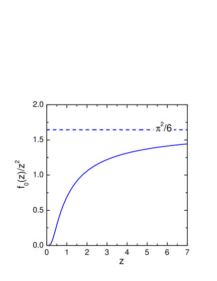
Figure 1: $f_{0}(z)/z^{2}$, cf. eq. (70). Dash line demonstrates asymptotic behavior for $z\gg 1$.

Numerical evaluation of the integral (66) is demonstrated in Fig. 1,

$$J_{s}=\frac{g_{s}^{2}(m_{b}^{*})^{2}z^{2}}{12\beta_{s}^{3/2}}r_{s}(z),\quad r_{s}(z)=\frac{6f_{0}(z)}{\pi^{2}z^{2}},\quad z=\frac{T}{m_{b}^{*}}.$$ (70)

The horizontal line shows the asymptotic behavior (68), $r_{s}(z)\rightarrow 1$ for $z\rightarrow\infty$. Below we will use a simplified eq. (68) to do analytic estimates for $T\gg m_{b}^{*}(T)$. In this case the quasiparticle approximation (valid for $\zeta\ll 1$) would work only for $g_{s}^{2}\ll 3\beta_{s}^{3/2}$. The latter inequality is not fulfilled for the $\sigma$ meson ($g_{s}\sim 10$).

Following (38), (70) we may evaluate the density of virtual (off-shell) bosons in the system, cf. eq. (33),

$$\rho_{b}=2m_{b}^{*}(T)(\phi_{c}^{\rm ext})^{2}=m_{b}^{*}(T)T^{2}r_{s}/(6\beta_{s}^{3/2}).$$ (71)

For $T\simeq m_{b}^{*}(T)\simeq m_{\pi}$, $\beta_{s}\simeq 1$, using numerical value of $J_{s}$ shown in Fig. 1 we obtain $\rho_{b}\simeq 0.1\rho_{0}$. It is worthwhile to notice that virtual bosons contribute to thermodynamic quantities, like phonons and diffusion modes do in the condensed matter physics. The calculation of their contribution to the energy, pressure, entropy, etc is however rather non-trivial task, see corresponding expressions for thermodynamic quantities in Appendix B.

4.2.3 Non-relativistic fermion distributions and density of fermion-antifermion pairs.

Assume $g_{s}\stackrel{{\scriptstyle\scriptstyle>}}{{\phantom{}{}_{\sim}}}1$, $T\stackrel{{\scriptstyle\scriptstyle>}}{{\phantom{}{}_{\sim}}}m_{b}^{*}(T)$ and $4J_{s}\ll m_{f}^{2}$. Then typical 4-momenta of fermions are

$$p^{2}\simeq m_{f}^{2}\pm O\left(\sqrt{J_{s}}m_{f}\right),$$ (72)

as we will show it below, see after (75), (81). With the condition (72) fulfilled, we have $|p_{0}-m_{f}|\ll m_{f}$ and $|\vec{p}|\sim\sqrt{2m_{f}T}\ll m_{f}$ for typical energies and momenta. This means that conditions for the applicability of the non-relativistic approximation for fermions are satisfied.

If the condition (72) is fulfilled, we have $2J_{s}G_{2}\ll 1$. Then from (60) it follows that $G_{1}\simeq G_{2}$. Eqs (56) and (57) coincide, if one replaces $p^{2}\simeq m_{f}^{2}$ in squared brackets in (56), (57) (but not in the pole term $G_{f}^{0,R}$). The same equation also follows from (4.2.1), if one neglects there a small $4J_{s}^{2}G_{2}^{4}+8J_{s}G_{2}^{3}$ term, according to eq. (72).

In the non-relativistic limit for fermions eq. (62) is simplified as

$$G_{1}^{R}\simeq G_{2}^{R}\simeq\frac{p^{2}-m_{f}^{2}\pm\sqrt{(p^{2}-m_{f}^{2}+i0)^{2}-2\gamma_{s}^{2}}}{\gamma_{s}^{2}},$$ (73)

$$\gamma_{s}^{2}=8J_{s}m_{f}^{2}.$$

We suppressed terms of the order of $O(J_{s}/m_{f}^{2})$.

We find from (73) that the condition $4\sqrt{J_{s}}m_{f}\ll|p^{2}-m_{f}^{2}|$ that would permit us to use the quasiparticle approximation is not satisfied for typical values of fermion energies and momenta given by (72). Therefore, in the energy-momentum range of our interest we definitely deal with off-mass shell fermions described by regular Green functions.

The accuracy of the approximation $G_{1}\simeq G_{2}$ made to get (73), cf. eq. (84) below, is rather appropriate for temperatures $T\stackrel{{\scriptstyle\scriptstyle<}}{{\phantom{}{}_{\sim}}}T_{\rm bl.f}$. The parameter of the expansion is $2J_{s}G_{2}^{R}(T\leq T_{\rm bl.f})\leq\sqrt{J_{s}}/m_{f}\leq\frac{1}{2\sqrt{3}}$, see eq. (87) below.

The solution of eq. (73) that yields ${\rm Im}G_{f}^{R}>0$ should be omitted as unphysical one. Thus, for the energy-momentum region of our interest $|p^{2}-m_{f}^{2}|\stackrel{{\scriptstyle\scriptstyle<}}{{\phantom{}{}_{\sim}}}\sqrt{2\gamma_{s}^{2}}$ there remains only the lower sign ($-$) solution:

$${\rm Re}G_{1}^{R}\simeq{\rm Re}G_{2}^{R}\simeq\frac{p^{2}-m_{f}^{2}}{\gamma_{s}^{2}},$$

$${\rm Im}G_{1}^{R}\simeq{\rm Im}G_{2}^{R}\simeq-\frac{\sqrt{2\gamma_{s}^{2}-(p^{2}-m_{f}^{2})^{2}}}{\gamma_{s}^{2}}\Theta\left(2\gamma_{s}^{2}-(p^{2}-m_{f}^{2})^{2}\right).$$ (74)

As follows from (4.2.3), the fermion spectral function satisfies the full sum rule (241), if both regions $p^{2}>m_{f}^{2}$ and $p^{2}<m_{f}^{2}$ are taken into account. Thus, although we did approximations, their consistency is preserved. The Green function (4.2.3) is the regular function, opposite to the pole solution $G_{f}^{0,R}$.

Replacing (4.2.3) into (A.2) we find the 3-momentum fermion distribution

$$\widehat{n}_{f,(\pm)}(\vec{p})=\int^{2m_{f}\sqrt{J_{s}}/\epsilon_{p}}_{-2m_{f}\sqrt{J_{s}}/\epsilon_{p}}\frac{d\xi}{\pi}\frac{\sqrt{2\gamma_{s}^{2}-4\epsilon_{p}^{2}\xi^{2}}}{\gamma_{s}^{2}}\frac{(\xi+\epsilon_{p})+m_{f}\gamma_{0}}{\mbox{exp}[(\xi+\epsilon_{p}\mp\mu_{f})/T]+1},$$ (75)

where we introduced the variable $\xi=p_{0}-\epsilon_{p}$ and used that $|\xi|<2m_{f}\sqrt{J_{s}}/\epsilon_{p}\ll\epsilon_{p}\sim m_{f}$. We also have dropped the term $\propto\vec{p}\,\vec{\gamma}$, since it does not contribute to the particle density $\rho_{f,(\pm)}$ due to the angular integration and since $\mbox{Tr}\gamma_{0}\vec{\gamma}=0$. Doing further the replacement $\xi=-2m_{f}\sqrt{J_{s}}/\epsilon_{p}+Ty$ and using that $\epsilon_{p}>m_{f}\gg T$, we obtain

$$\widehat{n}_{f,(\pm)}(\vec{p}) \simeq \frac{(\epsilon_{p}m_{f}^{-1}+\gamma_{0})\sqrt{\epsilon_{p}}\,T^{3/2}}{2\pi m_{f}^{1/2}J_{s}^{3/4}}I_{2}\left(\frac{4m_{f}\sqrt{J_{s}}}{\epsilon_{p}T}\right)$$ (76)

$$\times \mbox{exp}\left[-\frac{\epsilon_{p}-2m_{f}\sqrt{J_{s}}/\epsilon_{p}\mp\mu_{f}}{T}\right],$$

$$I_{2}(x)=\int^{x}_{0}dye^{-y}\sqrt{y-y^{2}x^{-1}},\quad x=4m_{f}\sqrt{J_{s}}/(\epsilon_{p}T),$$ (77)

$$I_{2}(x) \simeq \frac{\pi}{8}x^{3/2}(1-\frac{x}{2})\,,\quad\mbox{for}\quad x\ll 1,$$ (78)

$$I_{2}(x) \simeq \frac{\sqrt{\pi}}{2}\,,\quad\mbox{fo}r\quad x\gg 1.$$

As we have mentioned, the condition $x\simeq 4\sqrt{J_{s}}/T\ll 1$ is not fulfilled within the high temperature limit, which we are interested here, for $g_{s}\gg 1$, cf. estimate of $J_{s}$, eq. (68). Thereby, we show the result in this limit only for the completeness of the consideration.

Replacing (76) into (248) we find the fermion-antifermion density for one fermion species:

$$\rho_{f,\bar{f}} \equiv \rho_{f,(+)}+\rho_{f,(-)}\simeq\left[\mbox{exp}(\mu_{f}/T)+\mbox{exp}(-\mu_{f}/T)\right]$$ (79)

$$\times \frac{2T^{3/2}}{\pi J_{s}^{3/4}m_{f}^{1/2}}\int\frac{d^{3}p}{(2\pi)^{3}}\mbox{exp}\left(\frac{x}{2}-\frac{\epsilon_{p}}{T}\right)\epsilon_{p}^{1/2}I_{2}(x).$$

Subsequent integration yields

$$\frac{\rho_{f,(\pm)}}{\rho_{{\rm Bol},(\pm)}}\simeq\frac{T^{3/2}}{\pi J_{s}^{3/4}}I_{2}\left(\frac{4\sqrt{J_{s}}}{T}\right)\mbox{exp}\left[\frac{2\sqrt{J_{s}}}{T}\right],$$ (80)

$$\rho_{f,(\pm)}\simeq\frac{m_{f}^{3/2}T^{3}}{\sqrt{2}\pi^{5/2}J_{s}^{3/4}}I_{2}\left(\frac{4\sqrt{J_{s}}}{T}\right)\mbox{exp}\left[\frac{-m_{f}\pm\mu_{f}+2\sqrt{J_{s}}}{T}\right].$$ (81)

Integrating we have set in $\epsilon_{p}\simeq m_{f}+\vec{p}^{\,\,2}/(2m_{f})$ in the exponential factor and $\epsilon_{p}\simeq m_{f}$ in other values. At this instant we are able to support our above used estimate of typical fermion momenta given by (72).

In the limit $\sqrt{J_{s}}/T\rightarrow 0$ (i.e. for $g_{s}\rightarrow 0$, cf. eq. (68)) the ratio (80) of the particle/antiparticle density to the density of the Boltzmann gas (given by eq. (50)) tends to the unity. With the growth of the parameter $\sqrt{J_{s}}/T$ the ratio (80) monotonously increases. Thus the density of fermion-antifermion pairs is exponentially increased compared to the standard Boltzmann value.

The result (81) can be interpreted with the help of two new relevant quantities

$$m_{f,(+)}^{*}(T)=m_{f}\left(1-\frac{\mu_{f}}{m_{f}}-\frac{2\sqrt{J_{s}}}{m_{f}}\right),\quad 2\sqrt{J_{s}}\ll m_{f},$$ (82)

and

$$m_{f,(-)}^{*}(T)=m_{f}\left(1+\frac{\mu_{f}}{m_{f}}-\frac{2\sqrt{J_{s}}}{m_{f}}\right),\quad 2\sqrt{J_{s}}\ll m_{f}.$$ (83)

These quantities have the meaning of effective fermion and antifermion masses. However, contrary to the usually introduced effective masses, quantities (82), (83) enter only the exponent in the expression (79). We see that $m_{f,(+)}^{*}(T)$ and $m_{f,(-)}^{*}(T)$ decrease with increase of the intensity of the multiple scattering $J_{s}$. The latter value rises with the temperature, cf. eq. (68). In case of the non-zero baryon density the antifermion effective mass proves to be slightly higher than the fermion effective mass. Thus, for $\mu_{f}\neq 0$ the fermion mass-shell is blurred a bit more intensively than the antifermion mass-shell.

Were eq. (80) correct also for sufficiently large values of $J_{s}$, we could estimate a value

$$J_{s}=J_{s,\rm n.rel}^{({\rm bl.f})}(T_{\rm bl.f}^{s,\rm n.rel})\simeq(m_{f}-\mu_{f})^{2}/4,$$ (84)

at which the effective fermion mass (82) would vanish. $T_{\rm bl.f}^{s,\rm n.rel}$ would be then the typical temperature demonstrating a complete blurring of the gap between fermion and antifermion continua. Within the non-relativistic approach from (68) and (84) we would get

$$T_{\rm bl.f}^{s,\rm n.rel}\simeq\sqrt{3}\beta_{s}^{3/4}g_{s}^{-1}(m_{f}-\mu_{f})r_{s}^{-1/2}(T_{\rm bl.f}^{s,\rm n.rel}).$$ (85)

Here the correction factor $r_{s}$ takes into account deviation of the numerical value of the integral (66) from its asymptotic value (68).

However for $T>T_{\rm bl.f}^{s,\rm n.rel}$ the non-relativistic approximation for fermions is definitely incorrect, since the exponential factor in (81) arose from fermion occupations, which in any case should be less than unity, whereas for $T=T_{\rm bl.f}^{s,\rm n.rel}$ this factor has already reached the unity. In reality, as we show below, the non-relativistic approximation fails at still smaller temperatures. Thereby, we supplied here corresponding artificial values by an additional index “${\rm n.rel}$”.

The absolute maximum value of the density, which could be achieved in the region of the validity of the non-relativistic approximation, can be estimated with the help of the replacement of the exponential factor in (81) by unity. Then we evaluate

$$\rho_{f,(\pm)}^{\rm max}\simeq\frac{m_{f}^{3/2}T^{3}}{2^{3/2}\pi^{2}J_{s}^{3/4}}\rightarrow\frac{3^{3/4}\beta_{s}^{9/8}m_{f}^{3/2}T^{3/2}}{\pi^{2}g_{s}^{3/2}},$$ (86)

where we have used eq. (68). For $T\simeq m_{\pi}$, $g_{s}\simeq 10$, $\beta_{s}\simeq 1$, $m_{f}\simeq 6.7m_{\pi}$ we estimate $2\rho_{f,\bar{f}}^{\rm max}\simeq\rho_{0}$.

4.2.4 Relativistic fermion distributions and density of fermion-antifermion pairs. Blurred hadron continuum

An exponential smallness of fermion 3-momentum distributions disappears, if typical energies satisfy the condition $p_{0}\pm\mu_{f}\stackrel{{\scriptstyle\scriptstyle<}}{{\phantom{}{}_{\sim}}}T\ll m_{f}$. Thereby, and since we consider $|\mu_{f}|\ll T$, to keep the $\mu_{f}$ dependence in equations becomes even less important in this energy regime. Thus we further consider the case of the hadron vacuum. ${\rm Im}G_{2}$ is non-zero at $p_{0}$ near $0$ only for $J_{s}>m_{f}^{2}/12$, as it follows from eq. (65). This means that such small energies are present with a high probability only for $J_{s}\stackrel{{\scriptstyle\scriptstyle>}}{{\phantom{}{}_{\sim}}}m_{f}^{2}/12$. For $p_{0}\ll m_{f}$ the non-relativistic approximation, which we used above dealing with the fermion energies $p_{0}$ near the mass shell, becomes invalid. Thus, for $J_{s}\stackrel{{\scriptstyle\scriptstyle>}}{{\phantom{}{}_{\sim}}}m_{f}^{2}/12$ we should adopt the fully relativistic approach in order to incorporate the region of small fermion energies. If $p_{0},q_{0}\ll\sqrt{J_{s}}$ ($q_{0}$ is the boson energy variable in the diagrams (8), (33)), one may drop the energy dependence of the fermion Green function at all in the calculation of the fermion 3-momentum distribution, where typical energies $p_{0}$ are $\sim T$. The typical fermion 3-momentum is there $|\vec{p}|\sim m_{N}\gg|\vec{q}|\sim(T,\sqrt{2m_{b}^{*}T})$, see eq. (91) below. Thereby the STL approximation continues to hold in the given regime.

The condition of appearance of a non-trivial contribution to the imaginary part of $G_{2}$ for small values $p_{0}\stackrel{{\scriptstyle\scriptstyle<}}{{\phantom{}{}_{\sim}}}T$,

$$J_{s}^{\rm bl.f}(T_{\rm bl.f}^{s})\simeq m_{f}^{2}/12$$ (87)

determines the characteristic temperature of the complete blurring of the gap between fermion-antifermion continua. Within the fully relativistic approach for fermions, from (68), (70), (87) we evaluate the typical temperature of the blurring of the fermion vacuum,

$$T_{\rm bl.f}^{s}\simeq\beta_{s}^{3/4}g_{s}^{-1}m_{f}r_{s}^{-1/2}(T_{\rm bl.f}^{s}),\quad\mbox{for}\quad T_{\rm bl.f}^{s}\stackrel{{\scriptstyle\scriptstyle>}}{{\phantom{}{}_{\sim}}}m_{b}^{*}(T_{\rm bl.f}^{s}),$$ (88)

for the heavy fermion - scalar boson system under consideration. If one assumes $r_{s}(T_{\rm bl.f}^{s})\simeq r_{s}(T_{\rm bl.f}^{s,\rm n.rel})$, the quantity (88) is $1/\sqrt{3}$ times smaller than the artificial value (85) estimated above beyond the region of the validity of the non-relativistic approximation for fermions. We would like to draw attention to the fact that the limit $T_{\rm bl.f}^{s}\ll m_{b}^{*}(T_{\rm bl.f}^{s})$ is never realized, since $J_{s}$ is exponentially suppressed in this case, cf. (69). The opposite limit $T_{\rm bl.f}^{s}\gg m_{b}^{*}(T_{\rm bl.f}^{s})$ can be realized, only if the bare boson mass is rather small, namely $T_{\rm bl.f}^{s}\stackrel{{\scriptstyle\scriptstyle>}}{{\phantom{}{}_{\sim}}}m_{b}$, cf. next two subsections. Otherwise we have

$$T_{\rm bl.f}^{s}\sim m_{b}^{*}(T_{\rm bl.f}^{s}),$$ (89)

and the problem of the determination of $T_{\rm bl.f}^{s}$ is then a coupled-channel problem of a simultaneous evaluation of quantities $T_{\rm bl.f}^{s}$ and $m_{b}^{*}(T_{\rm bl.f}^{s})$.

Now we may find the fermion 3-momentum distribution for $J_{s}>J_{s}^{\rm bl.f}\simeq m_{f}^{2}/12$ (i.e., for $T>T_{\rm bl.f}^{s}$). Let us first consider only the contribution of the energy region $p_{0}\ll\sqrt{J_{s}}$. For typical values $p_{0}\sim T$, for the case $T\ll\sqrt{J_{s}}$, we may put $p_{0}=0$ in the expression for ${\rm Im}G_{2}$. Then we obtain the additional contribution of this energy region to the 3-momentum fermion distribution

$$\delta\widehat{n}_{f,(\pm)}(\vec{p})\simeq-\int_{0}^{\sqrt{J_{s}}}\frac{dp_{0}{\rm Im}G_{2}^{R}(p_{0}=0)}{\pi}\frac{(p_{0}+m_{f}\gamma_{0})}{e^{p_{0}/T}+1}$$

$$\simeq-\frac{{\rm Im}G_{2}^{R}(p_{0}=0)}{\pi}\left(T^{2}\frac{\pi^{2}}{12}+\gamma_{0}Tm_{f}\mbox{ln}2\right),$$ (90)

and to the fermion-antifermion density (one species of fermion)

$$\delta\rho_{f,(\pm)}(p_{0}\stackrel{{\scriptstyle\scriptstyle<}}{{\phantom{}{}_{\sim}}}T)=\frac{T^{2}}{6\pi}\int_{0}^{|\vec{p}_{\rm max}|}\vec{p}^{\,2}d|\vec{p}|\frac{\sqrt{12m_{f}^{2}J_{s}-4J_{s}\vec{p}^{\,2}-(\vec{p}^{\,2}+m_{f}^{2})^{2}}}{2m_{f}^{2}J_{s}(5+\frac{\vec{p}^{\,2}}{m_{f}^{2}}+\frac{4J_{s}}{m_{f}^{2}})},$$ (91)

$$\vec{p}_{\rm max}^{\,2}=-m_{f}^{2}-2J_{s}+\sqrt{4J_{s}^{2}+16J_{s}m_{f}^{2}},$$

where we used eq. (65). We see that for $J_{s}>J_{s}^{\rm bl.f}$ the fermion sub-system represents a rather dense packing of fermion-antifermion pairs ($J_{s}\geq J_{s}^{\rm bl.f}$ corresponds to the filling of a Fermi sea, $\vec{p}_{\rm max}=0$ for $J_{s}=J_{s}^{\rm bl.f}$). This is rather similar to the standard Fermi distribution at zero temperature but in our case fermion width effect is significant and the Fermi momentum $|\vec{p}_{\rm max}|$ has a different value. Moreover, effective fermion and antifermion Fermi seas exist simultaneously in our case.

In order to come to the quadratic equation from the fourth order one (see eq. (4.2.1)) we assumed that $2J|G_{2}|\ll 1$. For $p_{0}\simeq 0$ and, e.g., for $J_{s}\simeq 2J_{s}^{({\rm bl.f})}$ we have $|\vec{p}_{\rm max}|\simeq m_{f}/\sqrt{3}$ and, as it follows from eq. (62), $2J|{\rm Re}G_{2}|\simeq 1/3$. For $J_{s}\gg m_{f}^{2}$, $|{\rm Re}G_{2}^{R}|\sim 1/(2J_{s})$ and $2J|{\rm Re}G_{2}|\simeq 1$. Thus, we may continue to use eqs (62), (65) also in relativistic energy region (even for $J_{s}\gg m_{f}^{2}$ for qualitative estimates).

For $T$ in the vicinity of $T^{s}_{\rm bl.f}$ ($J_{s}-J_{s}^{\rm bl.f}\ll J_{s}^{\rm bl.f}$) using that $|\vec{p}_{\rm max}|=0$ for $J_{s}=J_{s}^{\rm bl.f}$ and expanding in (91) all quantities in small difference $J_{s}-J_{s}^{\rm bl.f}$ we obtain $\vec{p}_{\rm max}^{\,2}=36(J_{s}-J_{s}^{\rm bl.f})/7$ and

$$\delta\rho_{f,(\pm)}(p_{0}\stackrel{{\scriptstyle\scriptstyle<}}{{\phantom{}{}_{\sim}}}T)=\frac{81\sqrt{3}T^{2}(J_{s}-J_{s}^{\rm bl.f})^{2}}{112\sqrt{7}m_{f}^{3}}\Theta(J_{s}-J_{s}^{\rm bl.f}).$$ (92)

Notice that the total value $\rho_{f,(\pm)}$ does not tend to zero for $J_{s}=J_{s}^{\rm bl.f}\simeq m_{f}^{2}/12$. Indeed, one should still add to (92) the contribution of the energy region near the mass-shell, which we have estimated above within the non-relativistic approximation, see (81).

Suppose $g_{s}\simeq 10$, as for the $\sigma NN$ interaction, and $m_{f}=m_{N}\simeq g_{s}f_{\pi}$. Assuming $m_{b}^{*}(T)$ being significantly less than $T$ and using (68) thereby, we would get $T_{\rm bl.f}^{s,0}\simeq 93$ MeV for $\beta_{s}\simeq 1$, see (88). From (81) for two fermion (nucleon) species and for $T=T_{\rm bl.f}^{s,0}\simeq 93$ MeV, we then estimate $\rho_{N,\bar{N}}=2\rho_{f,\bar{f}}(p_{0}\sim m_{f})\simeq 4\rho_{f,(+)}(p_{0}\sim m_{f})\simeq 0.01\rho_{0}$. This is a tiny quantity. It means that in reality we still have $m^{*}_{b}(T)\simeq m_{b}$ at such a temperature. Thus the estimate $T_{\rm bl.f}^{s,0}\simeq 93$ MeV is not relevant, e.g., for the $N\sigma$ system, since the bare mass of $\sigma$ is $(500\div 600)$ MeV, i.e. much higher than $93$ MeV. We introduced a superscript ${}^{\prime\prime}0^{\prime\prime}$ to indicate this artificial feature.

The $\sigma$ meson has a large bare mass. Therefore we actually deal here with a coupled-channel problem, see eq. (89). In presence of nucleon-antinucleon pairs the effective mass of the $\sigma$ meson decreases that permits an extra production of pairs. The value of the nucleon pair density $\rho_{N,\bar{N}}$, at which the nucleon continuum is blurred, proves to be much smaller than the density that is necessary to reach the deconfinement transition at such a low temperature. Thus we should incorporate the factor $r_{s}<1$, cf. eq. (70). We will correct above estimate after evaluation of the value $m_{\sigma}^{*}(T)$, see below. Also, as we shall see below, with inclusion of correlation effects the effective coupling constant $g^{*}_{s}$ becomes smaller than $g_{s}$ that results in an increase of the value $T_{\rm bl.f}^{\sigma}$.

For artificially large values $J_{s}(T)\gg m_{f}^{2}$ using (91), (68) we estimate $\vec{p}_{\rm max}^{\,\,2}\simeq 3m_{f}^{2}$ and

$$\rho_{f,(\pm)}\simeq\frac{3T^{2}m_{f}^{4}}{128J_{s}^{3/2}}\rightarrow\frac{3^{5/2}\beta_{s}^{9/4}m_{f}^{4}}{16g_{s}^{3}T}.$$ (93)

The contribution of the energy region near the mass shell evaluated above within the non-relativistic approximation should be omitted in this limit. Thereby we replaced $\delta\rho_{f,(\pm)}$ to $\rho_{f,(\pm)}$. Also one should bear in mind that in derivation (91) we have put $p_{0}=0$ in the estimate of ${\rm Im}G$, although for $J_{s}(T)\gg m_{f}^{2}$ the whole energy region is populated. Moreover, we suppressed $G_{3}$ term in (37) that might be incorrect for $\vec{p}^{\,\,2}\stackrel{{\scriptstyle\scriptstyle>}}{{\phantom{}{}_{\sim}}}m_{f}^{2}$. Thus (93) can be considered only as a very rough estimate.

Even at such high temperatures (for $J_{s}(T)\gg m_{f}^{2}$) we find no end point for the hadron world conjectured in [5] (the value $d\rho_{f,(\pm)}/dT$ has no singularity at finite $T$ in our case). Furthermore, we see that $\rho_{f,(\pm)}$ may even decrease with the temperature increase in this energy region. Maximum available density of fermions can be very roughly estimated equating (92) plus (81) (in the latter equation we take into account that the exponential factor should not exceed unity, see eq. (86)), and on the other hand (93), from where we find $J_{s}(\rho_{f}^{\rm max})\simeq 0.4m_{f}^{2}$, $T\simeq 204~{}$MeV, and $2\rho_{f,\bar{f}}^{\rm max}\simeq 10\rho_{0}$ for $g_{s}\simeq 10$. Although estimates of many works show that the quark deconfinement transition may occur at much smaller temperature for given high density, all of them are done within simplified assumptions. E.g., one often compares pressures of the quark-gluon and hadron gases to conclude about the possibility of the deconfinement transition. We found that the hadron phase represents in reality a strongly correlated state, where the number of effective hadron degrees of freedom is dramatically increased with the temperature following the increase of $J_{s}(T)$. Thereby, one may expect a smoothening of the transition. More likely, in this case the system up to rather high temperatures may represent a strongly correlated hadron-quark-gluon state rather than the pure quark-gluon or the pure hadron state.

Note that calculating $\widehat{\Sigma}_{f}$, cf. eq. (13), we omitted terms proportional to fermion occupations. These terms are as small as the ratio of the contribution of quantum fluctuations to thermal fluctuations:

$$\frac{\int A_{b}n_{f}(p_{0}+q_{0})\frac{d^{4}q}{(2\pi)^{4}}}{\int A_{b}n_{b}(q_{0})\frac{d^{4}q}{(2\pi)^{4}}}<\frac{\int A_{b}\frac{d^{4}q}{(2\pi)^{4}}}{\int A_{b}n_{b}(q_{0})\frac{d^{4}q}{(2\pi)^{4}}}.$$ (94)

We also notice that the value $J_{s}^{({\rm bl.f})}$ evaluated within the relativistic approach is smaller than the quantity $J_{s,\rm n.rel}^{({\rm bl.f})}$ that would follow from the non-relativistic estimation outside the region of its validity.

4.2.5 Boson spectrum in the regime of non-relativistic fermions. Possibility of hot Bose condensation

We discussed the behavior of fermion Green functions and self-energies. Now let us evaluate the boson self-energy and find the boson spectrum. We will continue to exploit the high temperature limit ($T\stackrel{{\scriptstyle\scriptstyle>}}{{\phantom{}{}_{\sim}}}m^{*}_{b}(T)$) using fermion Green functions obtained in the STL approximation. Let us also assume, as before, that $G_{3}=0$, $G_{1}^{R}\simeq G_{2}^{R}$, and that boson 4-momenta $q_{0},|\vec{q}|$ are rather small ($q_{0},|\vec{q}|\ll m_{f}$, see estimation below). Then, dropping in eq. (16) a small term, which does not depend on thermal fermion occupations, and expanding (16) in $q_{0}$, $|\vec{q}|$ we find

$${\rm Re}\Sigma_{b}^{R}(q)\simeq-16g^{2}_{s}\int\frac{d^{3}p}{(2\pi)^{3}}\int_{0}^{\infty}\frac{dp_{0}}{(2\pi)}(p^{2}+m_{f}^{2}){\rm Im}G_{2}^{R}(p)$$

$$\times[{\rm Re}G_{2}^{R}(p)n_{f,(+)}(p_{0})+{\rm Re}G_{2}^{R}(-p)n_{f,(-)}(p_{0})]$$

$$-8g^{2}_{s}\int\frac{d^{3}p}{(2\pi)^{3}}\int_{0}^{\infty}\frac{dp_{0}}{(2\pi)}\left[\frac{d^{2}{\rm Re}G_{2}^{R}(p)}{dp^{\mu}dp^{\nu}}n_{f,(+)}(p_{0})+\frac{d^{2}{\rm Re}G_{2}^{R}(-p)}{dp^{\mu}dp^{\nu}}n_{f,(-)}(p_{0})\right]$$

$$\times q^{\mu}q^{\nu}(p^{2}+m_{f}^{2}){\rm Im}G_{2}^{R}(p)$$

$$-16g^{2}_{s}\int\frac{d^{3}p}{(2\pi)^{3}}\int_{0}^{\infty}\frac{dp_{0}}{(2\pi)}\left[\frac{d{\rm Re}G_{2}^{R}(p)}{dp^{\mu}}n_{f,(+)}(p_{0})+\frac{d{\rm Re}G_{2}^{R}(-p)}{dp^{\mu}}n_{f,(-)}(p_{0})\right]$$

$$\times q^{\mu}\cdot qp{\rm Im}G_{2}^{R}(p).$$ (95)

In our case according to (62) ${\rm Re}G_{2}^{R}(p)={\rm Re}G_{2}^{R}(-p)$ and eq. (4.2.5) is still simplified.

Let us first follow the approximation of non-relativistic fermions, $2\sqrt{J_{s}}\ll m_{f}$. With the help of eq. (4.2.3), doing the replacement $\xi=p_{0}-\epsilon_{p}$, for $\xi\ll\epsilon_{p}$, and then introducing the variable $\xi=-2m_{f}\sqrt{J_{s}}/\epsilon_{p}+Ty$ we get

$${\rm Re}\Sigma_{b}^{R}\simeq-\frac{2g^{2}_{s}\rho_{f,\bar{f}}}{\sqrt{J_{s}}}\left[1-\frac{T}{2\sqrt{J_{s}}}I_{3}\left(\frac{4\sqrt{J_{s}}}{T}\right)I_{2}^{-1}\left(\frac{4\sqrt{J_{s}}}{T}\right)\right]$$

$$+\alpha_{s}(q_{0}^{2}-\frac{1}{2}\vec{q}^{\,2}),$$ (96)

where we also used that $|\vec{p}|\sim\sqrt{2m_{f}T}\ll m_{f}$ and we have put $\epsilon_{p}\simeq m_{f}$ everywhere except the exponential factor $\mbox{exp}(-\epsilon_{p}/T)$. The quantity $\rho_{f,\bar{f}}$ is the fermion-antifermion density for one fermion species, given by eq. (80), the parameter

$$\alpha_{s}=\frac{2g^{2}_{s}\rho_{f,\bar{f}}}{J_{s}m_{f}}$$ (97)

is associated with the renormalization of the boson quasiparticle wave function, cf. eq. (67),

$$I_{3}(x)=\int^{x}_{0}dye^{-y}y\sqrt{y-y^{2}/x}.$$ (98)

In the limit cases we get

$$I_{3}(x)\simeq\frac{\pi}{16}x^{5/2}(1-\frac{5x}{8})\,,\quad\mbox{for}\quad x\ll 1,$$

$$I_{3}(x)\simeq\frac{3\sqrt{\pi}}{4}\,,\quad\mbox{for}\quad x\gg 1.$$ (99)

Thus

$${\rm Re}\Sigma_{b}^{R}(q) \simeq -\frac{g_{s}^{2}\rho_{f,\bar{f}}}{T}+\alpha_{s}(q_{0}^{2}-\frac{1}{2}\vec{q}^{\,2}),\quad\mbox{for}\quad x\simeq\frac{4\sqrt{J_{s}}}{T}\ll 1,$$ (100)

whereas in the high temperature limit under consideration

$${\rm Re}\Sigma_{b}^{R}(q) \simeq -\frac{2g_{s}^{2}\rho_{f,\bar{f}}}{\sqrt{J_{s}}}+\alpha_{s}(q_{0}^{2}-\frac{1}{2}\vec{q}^{\,2}),\quad\mbox{for}\quad x\simeq\frac{4\sqrt{J_{s}}}{T}\gg 1.$$ (101)

As follows from eq. (68), the limit $x\gg 1$ is indeed fulfilled, if coupling is strong ($g_{s}\gg 1$). In the approximation (249), $\mu_{f}/T\ll 1$, the real part of the boson self-energy does not depend on $\mu_{f}$ up to $O(\mu_{f}^{2}/T^{2})$ terms. Comparing $q$-independent and $q$-dependent terms in eqs (100) and (101) we see that expansions hold up to rather large values of $q_{0}^{2}$ and $\vec{q}^{\,\,2}$: $q_{0}^{2},\vec{q}^{\,\,2}\ll\sqrt{J_{s}}m_{f}\sim m_{f}^{2}/\sqrt{12}$ for $T\sim T_{\rm bl.f}^{s}$.

Assuming the validity of the quasiparticle approximation for bosons (${\rm Im}\Sigma_{b}^{R,(0)}\rightarrow 0$), we find the spectrum of boson excitations that takes the form (67) with

$$\beta_{s}=(1-\frac{1}{2}\alpha_{s})/(1-\alpha_{s}).$$ (102)

The wave function renormalization parameter $\alpha_{s}$ yields corrections to the $\omega^{2}$ and $\vec{q}^{\,2}$ terms.

The value

$$m_{b}^{*2}(T)\simeq(1-\alpha_{s})^{-1}\left[m_{b}^{2}-\frac{2g_{s}^{2}\rho_{f,\bar{f}}}{\sqrt{J_{s}}}\left(1-\frac{TI_{3}(x)}{2\sqrt{J_{s}}I_{2}(x)}\right)\right]$$ (103)

has the meaning of the squared effective boson mass. For the most interesting case, $x\gg 1$, we obtain

$$m_{b}^{*2}(T)\simeq m_{b}^{2}(1-\alpha_{s})^{-1}\left(1-\frac{2g_{s}^{2}\rho_{f,\bar{f}}}{m_{b}^{2}\sqrt{J_{s}}}\right),\quad 4\sqrt{J_{s}}\gg T.$$ (104)

Thus the effective boson mass achieves zero at some critical temperature $T_{\rm cb}$, being determined by the condition

$$\sqrt{J_{cs}^{(b)}(T_{\rm cb}^{s})}=\frac{2g_{s}^{2}\rho_{f,\bar{f}}(T_{\rm cb}^{s})}{m_{b}^{2}}.$$ (105)

Assuming that the non-relativistic approximation for fermions is fulfilled up to $T\sim T_{\rm cb}^{s}$ we estimate

$$\rho_{f,\bar{f}}(T_{\rm cb}^{s})=\frac{m_{b}^{2}T_{\rm cb}^{s}}{4\sqrt{3}\beta_{s}^{3/4}g_{s}}.$$ (106)

For $T_{\rm cb}^{s}\stackrel{{\scriptstyle\scriptstyle>}}{{\phantom{}{}_{\sim}}}T^{s}_{\rm bl.f}$ we have $\alpha_{s}\propto m_{b}^{2}/m_{f}^{2}\ll 1$ and $\beta_{s}\simeq 1+\frac{1}{2}\alpha_{s}$. To get expression (106) we used eq. (68). Note that at $T=T_{\rm cb}^{s}$ the correction factor $r_{s}=1$. For $m_{\sigma}\simeq 600$ MeV, $T^{s}_{\rm cb}\simeq m_{\pi}$, $g_{s}\simeq 10$, $\alpha_{s}=0$ we estimate $\rho_{N,\bar{N}}\simeq 0.7\rho_{0}$.

For $T>T_{\rm cb}^{s}$ the value $m_{b}^{*2}(T)$ becomes negative leading to the instability of the spectrum. The stability is recovered due to the appearance of the $s$-wave Bose condensation of the classical scalar field. Such a condensation can be called a hot Bose condensation (HBC), since it arises for the temperature $T>T_{\rm cb}^{s}$, rather than for $T<T_{\rm cb}^{s}$. As the consequence of the strong boson-fermion-antifermion interaction, the number of fermion degrees of freedom is dramatically increased that, on the other hand, results in the increase of the boson abundance. Boson degrees of freedom feel a lack of the phase space for energies and momenta $\sim T$ and a part of them is forced to occupy the coherent condensate state, thereby.

Let us now show that the quasiparticle approximation for bosons, which we have assumed to be valid exploiting (67), is, indeed, fulfilled in a wide temperature range. For that let us evaluate ${\rm Im}\Sigma_{b}^{R}$. Within the validity of the non-relativistic approximation for fermions, one has $2\sqrt{J_{s}}\ll m_{f}$. Then from (17) and (4.2.3) we find

$${\rm Im}\Sigma_{b}^{R}(q)\simeq-\frac{g^{2}_{s}}{8m_{f}^{4}J_{s}^{2}}\int\frac{d^{4}p}{(2\pi)^{4}}\sqrt{2\gamma_{s}^{2}-\left((p_{0}+q_{0})^{2}-\epsilon_{\vec{p}+\vec{q}}^{2}\right)^{2}}$$ (107)

$$\times \left(p^{2}+m_{f}^{2}+pq\right)\sqrt{2\gamma_{s}^{2}-\left(p^{2}_{0}-\epsilon_{p}^{2}\right)^{2}}$$

$$\times \left[\frac{1}{\mbox{exp}[(p_{0}-\mu_{f})/T]+1}-\frac{1}{\mbox{exp}[(p_{0}+q_{0}-\mu_{f})/T]+1}\right].$$

We see that in the critical point of the HBC ($q_{0}=0$) the squared bracketed term vanishes and, thereby, the boson width also vanishes. Thus in the problem of the determination of the critical point of the HBC one, indeed, may use the quasiparticle approximation for bosons.

Now let us consider finite but rather small values of $q_{0}$ and $|\vec{q}|$. For $q_{0}\ll T$, $|\vec{q}|\ll\sqrt{m_{f}T}$ we may drop the $q$-dependence everywhere except particle occupation factors. Separating fermion particle and antiparticle contributions, with the help of the replacement $p_{0}=\epsilon_{p}-\frac{2m_{f}\sqrt{J_{s}}}{\epsilon_{p}}+Ty$, we obtain

$${\rm Im}\Sigma_{b}^{R}(q)\simeq-\frac{2g^{2}_{s}T^{2}\left[\mbox{exp}(\mu_{f}/T)+\mbox{exp}(-\mu_{f}/T)\right]e^{-q_{0}/T}\left(e^{q_{0}/T}-1\right)}{\pi J_{s}^{3/2}}$$ (108)

$$\times \int\frac{d^{3}p}{(2\pi)^{3}}e^{-\epsilon_{p}/T}\mbox{exp}\left(\frac{2m_{f}\sqrt{J_{s}}}{\epsilon_{p}T}\right)I_{4}\left(\frac{4m_{f}\sqrt{J_{s}}}{\epsilon_{p}T}\right),$$

$$I_{4}(x)=\int^{x}_{0}e^{-y}dy\left(y-y^{2}/x\right)=e^{-x}\left(1+\frac{2}{x}\right)+1-\frac{2}{x},$$ (109)

$$I_{4} \simeq \frac{x^{2}}{2}\,,\quad\mbox{for}\quad x\ll 1,$$

$$I_{4} \simeq 1-\frac{2}{x}\,,\quad\mbox{for}\quad x\gg 1.$$ (110)

Finally, we find

$${\rm Im}\Sigma_{b}^{R} \simeq -\frac{1}{2}\alpha_{s}T^{1/2}J_{s}^{1/4}m_{f}I_{4}\left(\frac{4\sqrt{J_{s}}}{T}\right)$$ (111)

$$\times I_{2}^{-1}\left(\frac{4\sqrt{J_{s}}}{T}\right)e^{-q_{0}/T}\left(e^{q_{0}/T}-1\right).$$

Comparing (111) and (4.2.5) we see that in the high temperature limit under consideration, for $x\simeq\frac{4\sqrt{J_{s}}}{T}\gg 1$, and for $q_{0}^{2}\ll T\sqrt{J_{s}}$ one has $|{\rm Im}\Sigma_{b}^{R}|\ll|{\rm Re}\Sigma_{b}^{R}|$. The inequality $|{\rm Im}\Sigma_{b}^{R}|\ll|{\rm Re}\Sigma_{b}^{R}|$ also holds for $q_{0}\ll\sqrt{J_{s}}$ at $\frac{4\sqrt{J_{s}}}{T}\ll 1$. Thus, the quasiparticle approximation is, indeed, valid for bosons in a wide temperature range of our interest. For typical values $q_{0}\sim T$ we have $|{\rm Im}\Sigma_{b}^{R}|\ll|{\rm Re}\Sigma_{b}^{R}|$ in both limits $x\gg 1$ and $x\ll 1$. Thereby, we justified that above we correctly used the quasiparticle approximation to calculate $J_{s}$. On the other hand, the quasiparticle approximation fails for $|{\rm Im}\Sigma_{b}^{R}(q_{0}=m_{b}^{*}(T))|\stackrel{{\scriptstyle\scriptstyle>}}{{\phantom{}{}_{\sim}}}m_{b}^{*2}(T)$, that takes place in a narrow vicinity of the HBC critical point, but not in the critical point itself, where ${\rm Im}\Sigma_{b}^{R}=0$.

4.2.6 Hot Bose condensation in the regime of blurred fermion continuum.

For $J_{s}>J_{s}^{\rm bl.f}$ the fermion energy region $p_{0}\ll m_{f}$ is permitted. Due to that there appears an additional term in the boson self-energy. To find it let us consider the limit $J_{s}-J_{s}^{\rm bl.f}\ll J_{s}^{\rm bl.f}$, for $J_{s}>J_{s}^{\rm bl.f}$. Then still one has $G_{1}\simeq G_{2}$ with a reasonable accuracy. With the help of eq. (62) from (4.2.5) within the same set of approximations, which we have used to obtain eq. (91), we find

$$\delta{\rm Re}\Sigma_{b}^{R}(q) \simeq -\frac{36(\mbox{ln}2)g_{s}^{2}\delta\rho_{f,\bar{f}}(p_{0}\stackrel{{\scriptstyle\scriptstyle<}}{{\phantom{}{}_{\sim}}}T)}{\pi^{2}T_{\rm bl.f}^{s}}\left(1-\frac{9}{4}\frac{q_{0}^{2}}{m_{f}^{2}}+\frac{3}{4}\frac{\vec{q}^{\,2}}{m_{f}^{2}}\right),$$ (112)

where $\delta\rho_{f,\bar{f}}(p_{0}\stackrel{{\scriptstyle\scriptstyle<}}{{\phantom{}{}_{\sim}}}T)=\delta\rho_{f,(+)}+\delta\rho_{f,(-)}$, see eq. (91). Eq. (112) yields the correction term to the effective boson mass (104)

$$m_{b}^{*2}(T)\simeq m_{b}^{2}(1-\alpha_{s})^{-1}\left(1-\frac{2g_{s}^{2}\rho_{f,\bar{f}}}{m_{b}^{2}\sqrt{J_{s}}}-\frac{36(\mbox{ln}2)g_{s}^{2}\delta\rho_{f,\bar{f}}(p_{0}\stackrel{{\scriptstyle\scriptstyle<}}{{\phantom{}{}_{\sim}}}T)}{\pi^{2}T_{\rm bl.f}^{s}m_{b}^{2}}\right),$$ (113)

where we dropped a numerically small contribution to the wave function renormalization from the region $p_{0}\stackrel{{\scriptstyle\scriptstyle<}}{{\phantom{}{}_{\sim}}}T$.

If the effective boson mass $m_{b}^{*}(T)$ achieves zero in the regime $T>T_{\rm bl.f}^{s}$, $T-T_{\rm bl.f}^{s}\ll T_{\rm bl.f}^{s}$, then the critical point of HBC is determined by the condition

$$m_{b}^{2}-\frac{2g_{s}^{2}\rho_{f,\bar{f}}(p_{0}\sim m_{f})}{\sqrt{J_{s}}}-\frac{36\mbox{ln}(2)g_{s}^{2}\delta\rho_{f,\bar{f}}(p_{0}\stackrel{{\scriptstyle\scriptstyle<}}{{\phantom{}{}_{\sim}}}T)}{\pi^{2}T_{\rm bl.f}^{s}}=0,$$ (114)

where we used eqs (101), (67) and (112).

Applying results for $N\bar{N}\sigma$ we should replace $\rho_{f,\bar{f}}\rightarrow 2\rho_{f,\bar{f}}=\rho_{N\bar{N}}$ and $\delta\rho_{f,\bar{f}}\rightarrow 2\delta\rho_{f,\bar{f}}=\delta\rho_{N\bar{N}}$ in boson self-energy terms to take into account two fermion species, i.e., neutrons and protons in the given case. Numerical estimate shows that for $m_{\sigma}\simeq 600$ MeV and $g_{s}\simeq 10$, the critical temperature of the HBC is $T_{\rm cb}^{s}\simeq 114$ MeV, $J_{cs}^{(b)}(T_{\rm cb}^{s})\simeq 1.5J^{\rm bl.f}_{s}(r_{s}=1)$, $\alpha_{s}(T_{\rm cb}^{s})\simeq 0.3$. As we mentioned, if the limit $T\gg m_{\sigma}^{*}(T)$ were fulfilled for $T\simeq T_{\rm bl.f}^{s}$, using (68) we would come back to the estimate $T_{\rm bl.f}^{s,0}\simeq m_{f}\beta_{s}^{3/4}/g_{s}\simeq 93$ MeV. However for such a temperature $m_{\sigma}^{*}$ is still close to the bare mass and one needs to use the opposite limit expression (69). Thereby, the value $T_{\rm bl.f}^{s}$ should be somewhat larger. Within a coupled channel estimate we find that the renormalized value $T_{\rm bl.f}^{s}\stackrel{{\scriptstyle\scriptstyle>}}{{\phantom{}{}_{\sim}}}m^{*}_{\sigma}(T_{\rm bl.f}^{s})$. Finally we find that $T_{\rm bl.f}^{s}\simeq 105$ MeV, that is only slightly less than $T_{\rm cb}^{s}$. Using instead of $g_{s}$ a smaller value of the effective coupling constant $g_{s}^{*}\simeq 0.7g_{s}$, as we estimate it below, we obtain higher values $T_{\rm bl.f}^{s}\simeq 150~{}$MeV and $T_{\rm cb}^{s}\simeq 160$ MeV. For smaller value $m_{\sigma}$ (e.g., for $500$ MeV instead of $600$ MeV) we would get smaller values of $T_{\rm bl.f}^{s}$ and $T_{\rm cb}^{s}$. With these variations we see that in all relevant cases $T_{\rm bl.f}^{s}$ and $T_{\rm cb}^{s}$ remain to be somewhere in the vicinity of the pion mass ($\sim 140$ MeV).

Please notice that in order to find a possible relation between the HBC and the chiral symmetry restoration one would need to consider both possibilities in the framework of the very same model, e.g., the linear $\sigma$-model, introducing meson self-interaction terms and the spontaneous symmetry breaking for the $\sigma$ vacuum at $T=0$. As an intriguing circumstance, let us mention that replacing $g_{\sigma}\simeq m_{N}/f_{\pi}$ (for $\sigma=f_{\pi}$, as it follows from the $\sigma$ model) into (88) and (85) we find $T_{\rm bl.f}^{s}=f_{\pi}$ and $T_{\rm bl.f}^{s,\rm n.rel}=\sqrt{3}f_{\pi}$ for $\beta_{s}\ll 1$. Namely in this range of temperatures one expects the chiral restoration phase transition, cf. [22]. We postpone a more detailed discussion of these questions to the future work.

For $T>T_{\rm cb}^{s}$, in the mean field approximation, the classical scalar field $\phi_{sc}$ is determined by the equation

$$m_{\rm MF}^{2}\phi_{sc}+\lambda_{s}^{\rm ef}\phi_{sc}^{3}=0,$$ (115)

$$m_{\rm MF}^{2}=m_{b}^{2}+{\rm Re}\Sigma_{b}^{R}(q\rightarrow 0)+\delta{\rm Re}\Sigma_{b}^{R}(q\rightarrow 0),$$

which has the solution $\phi_{sc}^{2}\simeq-(m_{\rm MF}^{2}/\lambda_{s}^{\rm ef})\Theta(-m_{\rm MF}^{2})$ for $T>T_{\rm cb}^{s}$. Here the value $\lambda_{s}^{\rm ef}>0$ is the effective boson self-interaction coupling constant,

$$L_{int}=-\lambda_{s}^{\rm ef}\phi_{sc}^{4}/4.$$ (116)

It arises since for $T>T_{\rm cb}^{s}$ one needs to add the condensate dependent terms to the one term $\Phi$-diagram. With inclusion of this interaction excitations become stable in presence of the condensate. In reality one also has an extra term in the Lagrangian, $L_{int}=-\lambda_{\rm vac}\phi_{sc}^{4}/4$, related to the vacuum boson-boson self-interaction. We for simplicity suppressed the latter.

The condensate field is the static field corresponding to the absence of real scalar particles with zero momentum. The contribution of the condensate to the free energy density becomes

$$\delta F(V,T)=-\frac{m_{\rm MF}^{4}(T)}{4\lambda_{s}^{\rm ef}}\Theta(T-T_{\rm cb}^{s})\propto-(T-T_{\rm cb}^{s})^{2}\Theta(T-T_{\rm cb}^{s}),$$ (117)

demonstrating typical second order phase transition behavior, however for $T>T_{\rm cb}^{s}$ rather than for $T<T_{\rm cb}^{s}$, as it would take place for the ordinary phase transition.

4.2.7 Boson abundance in matter and at infinity

The boson population in the medium is greatly enhanced with the increase of the temperature due to the decrease of the effective boson mass. Accordingly, the distribution function (A.2) has a sharp peak at small momenta $|\vec{q}|^{2}\stackrel{{\scriptstyle\scriptstyle<}}{{\phantom{}{}_{\sim}}}m_{b}^{*\,2}(T)/\beta_{s}$:

$$\frac{dN_{s}^{\rm med}}{d^{3}q/(2\pi)^{3}}=\mbox{Tr}\,\widehat{n}_{s,(\pm)}(\vec{q})=\frac{(1-\alpha_{s})^{-1}}{e^{\omega_{s}(\vec{q},T)/T}-1},\quad\mbox{for}\quad T<T_{\rm cb}^{s},$$ (118)

with $\omega_{s}(\vec{q},T)$ given by (67). Distributions of particles at infinity might be significantly different from distributions inside the matter. This depends on the scenario of the breakup stage. If breakup were sudden, then particle distributions at infinity would be given by [13, 14]

$$\frac{dN_{s}^{\infty}}{d^{3}q/(2\pi)^{3}}\simeq\frac{\sqrt{m_{s}^{2}+\vec{q}^{\,2}}}{\omega_{s}(\vec{q},T)(1-\alpha_{s})}\frac{dN_{s}^{\rm med}}{d^{3}q/(2\pi)^{3}},\quad\mbox{for}\quad T<T_{\rm cb}^{s}.$$ (119)

For sudden change of the system the particle momentum is conserved, whereas the particle energy might change. However the total energy is certainly conserved. Thus eq. (119) should be still supplemented by the requirement of the conservation of the total energy. The energy mismatch that arises at the breakup stage is compensated by the change of the energy of the particle collective flow.

For $T>T_{\rm cb}^{s}$, in the vicinity of the critical point the stable spectrum of excitations is determined by the equation

$$(1-\alpha_{s})\omega^{2}_{s}(\vec{q},T)\simeq m_{\rm MF}^{2}(T)+3\lambda_{s}^{\rm ef}(T)\phi_{sc}^{2}+(1-\frac{1}{2}\alpha_{s}(T))\vec{q}^{\,2},$$ (120)

for $\alpha_{s}<1$, $|\vec{q}|>0$. Here we used eq. (4.2.5) and added the contribution of the classical condensate field. The latter is found with the help of eq. (116), if one does there the variable replacement $\phi_{sc}\rightarrow\phi_{sc}+\phi^{\prime}$ to recover fluctuation-condensate coupling terms. To avoid a more cumbersome expression we dropped here a numerically small correction term to the wave function renormalization from the region $p_{0}\stackrel{{\scriptstyle\scriptstyle<}}{{\phantom{}{}_{\sim}}}T$.

For the temperature in the vicinity of $T_{\rm cb}^{s}$ the boson behaves as almost massless particle, $\omega^{2}\simeq\vec{q}^{\,2}$ (for $\alpha_{s}\ll 1$). This results in the enhancement of the production of soft bosons and in the corresponding enhancement of the total particle yield compared to that would be for the originally massive bosons.

Observation of a $\delta$-function-like peak in the meson distribution at zero momentum, if occurred, could be interpreted, as the fulfillment of the condition $T_{\rm b.up}\geq T_{\rm bc}$, where $T_{\rm b.up}$ is the temperature reached at the breakup stage. A significant enhancement of the meson distribution at small momenta $|\vec{p}|\stackrel{{\scriptstyle\scriptstyle<}}{{\phantom{}{}_{\sim}}}T$ can be interpreted as a signal of the closeness of $T_{\rm b.up}$ to the value $T_{\rm bc}$ (for $T_{\rm b.up}<T_{\rm bc}$), see also [23].

The HBC may appear only, if $T_{\rm cb}^{s}$ is less than the critical temperature for the deconfinement, $T_{\rm dec}$, since for $T>T_{\rm dec}$ there would occur a complete breakdown of the hadron vacuum. As we estimated $T_{\rm cb}^{s}\sim m_{\pi}$, and as we argued, at relevant rather small density the deconfinement is probably delayed up to a high temperature. Please notice that to simplify the consideration we disregarded in our analysis the quark-gluon contribution to hadron quantities, e.g., an extra decrease of meson masses due to the change of the quark condensate with the increase of the temperature.

Concluding, we treated the fermion-boson problem self-consistently. Fermions due to rescatterings on bosons acquire broad widths and, as the reaction on that, bosons decrease their masses.

The typical behavior of the logarithm of the ratio of the fermion density to the corresponding Boltzmann quantity as function of the temperature is shown in Fig. 2 for $T<T_{\rm cb}^{s}$. Moreover Fig. 2 demonstrates the temperature dependence of the effective scalar boson mass. We see a huge enhancement of $\mbox{ln}(\rho_{f}/\rho_{f,\rm Bol})$ and a drastic decrease of $m_{b}^{*}/m_{b}$ in the vicinity of $T=T_{\rm bl.f}^{s}$. At the critical point $m_{bt}^{*}/m_{b}$ reaches zero demonstrating possibility of the second order phase transition to the HBC state.

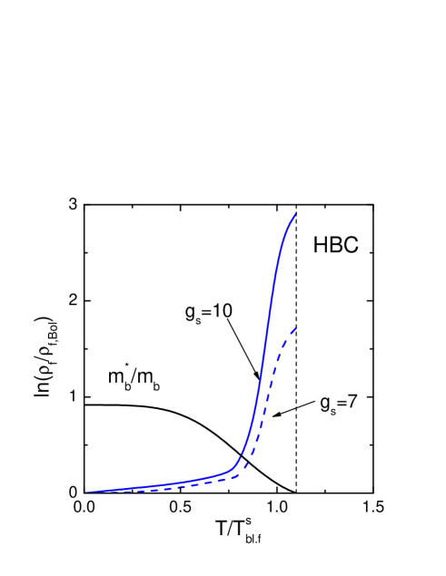
Figure 2: Logarithm of the ratio of the fermion density to the corresponding Boltzmann quantity for $g_{s}=10$ and $g_{s}=7$, and the effective scalar boson mass as functions of the temperature in units of $T_{\rm bl.f}^{s}$. The vertical dash-line indicates the area of the HBC.

4.3 Contribution of baryon resonances

Above we considered a simple example of the system consisting of heavy fermions of one species interacting with one kind of less massive scalar bosons. However at finite temperature together with nucleon/antinucleon states the high-lying baryon/antibaryon resonances, like $\Delta$ isobar, hyperons, etc, are also populated with some probability. Resonances interact with each other by boson exchanges, as well as by a residual interaction (including repulsive baryon-baryon correlations). To describe the multi-component system of the baryon/antibaryon resonances interacting with mesons we need to know coupling constants between different particle species. In general, Dyson equations for Green functions of different particles are coupled and the problem proves to be very complicated. Different meson exchanges may significantly contribute. E.g., for the $\Delta$ isobar the coupling in the pion channel is the dominant one. However the scalar channel might be also important. According to [24] $\sigma$ mesons interact with $\Delta$-isobars with the same universal coupling constant $g_{s}\simeq 10$. In case of $N^{*}(1440)$ one gets [25] $g_{\sigma NN^{*}}/g_{\sigma NN}\simeq 0.47$, $g_{\pi NN^{*}}/g_{\pi NN}\simeq 0.53g_{\sigma NN^{*}}/g_{\sigma NN}\simeq 0.25$.

4.3.1 Low temperature limit

As above, let us for simplicity first assume that baryon resonances couple by an exchange of only a scalar neutral boson ($s$). This simplification is sufficient to find particle distributions in the low temperature limit, $T\ll\mbox{min}\{m_{b},T_{\rm bl.f}\}$. Then we may still use eqs (A.2), (248), (18) for the given baryon resonance, however with $\widehat{\Lambda}_{f}^{0}$ operators being different in dependence on the spin of the baryon species. Calculating the resonance width we need to take into account in (14) various possible intermediate states, since the given resonance may decay to the virtual boson and to an another baryon resonance then absorbing back the virtual (off-mass shell) boson. Notice that we discuss only temperature effects. Just to simplify the consideration we artificially suppressed the widths terms surviving for $T=0$.

Let us present the density of the baryon resonance/antiresonance states of the fixed species $B^{*}$. In the low temperature limit using (3.2), (49), (50) we obtain

$$\rho_{B^{*},(\pm)}\simeq N_{B^{*}}\left(\frac{m_{B^{*}}T}{2\pi}\right)^{3/2}\mbox{exp}\left[-\frac{m_{B^{*}}\mp\mu_{B^{*}}}{T}\right]$$ (121)

$$+N_{B^{*}}\sum_{i}\left(\frac{m_{B^{*}_{i}}T}{2\pi}\right)^{3/2}\mbox{exp}\left[-\frac{m_{B^{*}_{i}}\mp\mu_{B^{*}_{i}}}{T}\right]\frac{g_{sB^{*}B^{*}_{i}}^{2}}{4\pi^{2}}I_{0s}\left(\frac{m_{B^{*}_{i}}}{m_{b}}\right).$$

$N_{B^{*}}$ is the degeneracy factor (e.g., $N_{n}=N_{p}=2$). The summation is performed over all possible states including the given baryon state ($B^{*}$), $m_{B^{*}}$ is the mass of the $B^{*}$ baryon resonance. For non-strange baryons with the same baryon number, as for the nucleon, we have $\mu_{B^{*}}=\mu_{N}$, if there is a permitted reaction channel: $B^{*}\leftrightarrow N+b^{virt}$. Here $b^{virt}$ is the virtual boson (in our model example it is a scalar boson, whereas in reality it also could be the pion, $\sigma$, $\omega$, etc). Second term in (121) is due to the diagram

(122)

where external double-lines correspond to the given resonance $B^{*}$ and internal solid line relates to the resonance $B^{*}_{i}$, including the given resonance $B^{*}$ and the nucleon state. In the latter case the self-energy term is the same as in eq. (8).

Thus, the baryon resonance density is substantially increased compared to the Boltzmann value. The term in eq. (121) relating to the decay of the given baryon resonance to the nucleon and the virtual boson ($i=n$ or $p$, solid line in (122)), has no suppression factor, as $e^{-(m_{B^{*}}-m_{N})/T}$. The latter factor would arise, if one worked in the framework of the quasiparticle picture. If $N_{B^{*}}g^{2}_{sB^{*}N}$ were larger than $N_{N}g^{2}_{sNN}$, the density of a high-lying resonance could be even higher than the nucleon density, showing a laser effect. Opposite, if $g_{sB^{*}_{i}B^{*}_{j}}$ were negligible for $i\neq j$, the laser enhancement would disappear and a high-lying resonance state would be less populated than the nucleon one. Nevertheless, in any case the resonance state proves to be more populated compared to the value determined by the corresponding Boltzmann expression.

4.3.2 High temperature limit

To proceed in the high temperature limit let us additionally assume that $g_{sB^{*}_{i}B_{j}^{*}}\neq 0$ only for $i=j$. Then in the non-relativistic approximation for the resonance, the density of a $B^{*}$ baryon resonance (and its anti-partner) is found with the help of eq. (81). We obtain

$$\rho_{B^{*},(\pm)}\simeq\frac{N_{B^{*}}m_{B^{*}}^{3/2}T^{3}}{2\sqrt{2}\pi^{5/2}J_{s,B^{*}}^{3/4}}\mbox{exp}\left[-\frac{m_{B^{*},(\pm)}^{*}(T)}{T}\right]I_{2}\left(\frac{4\sqrt{J_{s,B^{*}}}}{T}\right).$$ (123)

Here, in agreement with eq. (58) the intensity of the multiple scattering is

$$J_{s,B^{*}}=2g_{\sigma B^{*}B^{*}}^{2}\int\frac{d^{3}q}{(2\pi)^{3}}\int_{0}^{\infty}\frac{dq_{0}}{2\pi}A_{s,(+)}(q)n_{s,(+)}(q_{0}),$$ (124)

where we used that for scalar neutral bosons $A_{s,(+)}(q)=A_{s,(-)}(q)$ and $n_{s,(+)}(q_{0})=n_{s,(-)}(q_{0})$. The effective mass of the baryon resonance follows from expression (82):

$$m_{B^{*},(\pm)}^{*}(T)=m_{B^{*}}\left(1\mp\frac{\mu_{N}}{m_{B^{*}}}-\frac{2\sqrt{J_{s,B^{*}}}}{m_{B^{*}}}\right),\,\,\,\mbox{for}\,\,\,2\sqrt{J_{s,B^{*}}}\ll m_{B^{*}}.$$ (125)

Analogously, one rewrites expressions (92), (93) for the density of the baryon resonance in the relativistic energy region. Within the quasiparticle approximation for the boson using (101), (112) we obtain the effective boson mass:

$$m_{b}^{*2}(T)\simeq(1-\alpha_{s})^{-1}$$ (126)

$$\times\left[m_{b}^{2}-\sum_{i}\left(\frac{2g^{2}_{sB^{*}_{i}B^{*}_{i}}\rho_{B^{*}_{i}}(p_{0}\sim m_{B^{*}_{i}})}{\sqrt{J_{s,B^{*}_{i}}}}+\frac{36(\mbox{ln}2)g^{2}_{sB^{*}_{i}B^{*}_{i}}\delta\rho_{B^{*}_{i}}(p_{0}\stackrel{{\scriptstyle\scriptstyle<}}{{\phantom{}{}_{\sim}}}T)}{\pi^{2}T^{s}_{\rm bl.f}}\right)\right],$$

$$\alpha_{s}=\sum_{i}\frac{2g^{2}_{sB^{*}_{i}B^{*}_{i}}\rho_{B^{*}_{i}}(p_{0}\sim m_{B^{*}_{i}})}{J_{s,B^{*}_{i}}m_{B^{*}_{i}}},$$ (127)

The summation is over all baryons and antibaryons, $\rho_{B^{*}_{i}}$ is the corresponding baryon or antibaryon density. As in eq. (113), we dropped a numerically small correction term to the wave function renormalization from the region $p_{0}\stackrel{{\scriptstyle\scriptstyle<}}{{\phantom{}{}_{\sim}}}T$.

In the limiting cases of high and low temperatures we recover eqs (68), (69), now with the coupling constant $g_{\sigma B^{*}B^{*}}$ standing instead of $g_{s}$ and $\beta_{B^{*}}$, instead of $\beta_{s}$,

$$J_{s,B^{*}}=\frac{g_{\sigma B^{*}B^{*}}^{2}T^{2}}{12\beta_{B^{*}}^{3/2}}\,,\quad\mbox{for}\quad T\gg m_{b}^{*}(T),$$ (128)

and

$$J_{s,B^{*}}=\frac{g_{\sigma B^{*}B^{*}}^{2}T^{3/2}\sqrt{m_{b}^{*}}}{2^{3/2}\pi^{3/2}\beta_{B^{*}}^{3/2}}\mbox{exp}{\left(-m_{b}^{*}/T\right)}\,,\quad\mbox{for}\quad T\ll m_{b}^{*}(T).$$ (129)

We see that for $T\gg m_{b}^{*}(T)$ the intensity of the multiple scattering, $J_{s,B^{*}}$, of a high-lying baryon resonance would exceed that for the nucleon, $J_{s,N}$, if $g_{sB^{*}B^{*}}^{2}$ were larger than $g_{sNN}^{2}$. As follows from eq. (125), for $g_{sB^{*}B^{*}}^{2}/m_{B^{*}}^{2}>g_{sNN}^{2}/m_{N}^{2}$, the baryon continuum for the given high-lying baryon resonance would be blurred at a smaller temperature than for the nucleon. Please notice that such a relation between coupling constants is not fulfilled for the realistic hyperon-$\sigma$-nucleon interaction, cf. [27]. Nevertheless, using estimates [27] we conclude that resonances contribute essentially to the total baryon-antibaryon density for $T\sim T_{\rm bl.f}$. Moreover, we artificially suppressed all couplings except $g_{sB^{*}_{i}B_{j}^{*}}$ for $i=j$ that is certainly not the case in the reality. Also in reality $g_{sB^{*}_{i}B_{j}^{*}}\neq g_{sB^{*}_{j}B_{i}^{*}}$ for $i\neq j$ since $N_{B^{*}_{i}}\neq N_{B^{*}_{j}}$, that may stimulate in some cases a laser effect. A high-lying state might be more populated than a low-lying state (Note that, e.g., in case of the $\Delta$ isobar, i.e. $(\frac{3}{2},\frac{3}{2})$ resonance, one has $N_{\Delta}/N_{N}=4$, that works in favor of the laser effect).

Concluding, indeed, we deal with the hadron resonance porridge at a sufficiently large temperature.

4.4 Evaluation of correlation effects

Above we discussed properties of the system described within the simplest $\Phi$-derivable approximation with only one diagram (2). Exact fermion and boson self-energies are determined by diagrams (6) and (7) with one free and one exact vertices. In the low temperature limit vertex corrections are negligible. Thereby, we further consider the high temperature limit $T\stackrel{{\scriptstyle\scriptstyle>}}{{\phantom{}{}_{\sim}}}m_{b}^{*}(T)$. The equation for the vertex can be greatly simplified within the ladder re-summation:

(130)

that reads as

$$\widehat{V}_{\rm lad}(q_{1},p,p+q_{1})=\widehat{V}_{0}(q_{1})-\int\widehat{G}_{f}(p-q)\widehat{G}_{f}(p+q_{1}-q)$$

$$\times i\widehat{V}_{\rm lad}(q,p+q_{1}-q,p+q_{1})G_{b}(q)\widehat{V}_{\rm lad}(-q,p,p-q)$$

$$\times\widehat{V}_{\rm lad}(q_{1},p-q,p+q_{1}-q)\frac{d^{4}q}{(2\pi)^{4}},$$ (131)

the corresponding matrix indices are implied. We need $-,-,-$ and $+,+,+$ vertex functions of the same signs, since in the formalism that uses full Green functions, cf. [21], any extra full Green function $G^{-+}$ or $G^{+-}$ corresponds to the scattering process involving extra particle in the initial and the final state. These processes are suppressed, if the number of fermion-antifermion pairs is not too large. In the STL approximation, which we now exploit, we find

$$V_{\rm lad}^{---}\simeq\frac{g_{s}}{1+J_{s}(V_{\rm lad}^{---})(p^{2}+m_{f}^{2}+2\hbox{$/$}\kern-5.01563pt\hbox{$p$}m_{f})\left[{\rm Re}G_{1}(p)\right]^{2}},$$ (132)

where we also used the spin structure of fermion Green functions (37), within the ansatz $G_{3}=0$, assuming $G_{1}\simeq G_{2}$. The quantity $J_{s}(V_{\rm lad}^{---})$ is $J_{s}$ with the bare vertices $g_{s}$ replaced to the full vertices, see corresponding fat dots in (130). Thus, one may restrict the consideration to the first diagram (2) only if $(p^{2}+m_{f}^{2})J_{s}(V_{\rm lad}^{---})\left[{\rm Re}G_{1}(p)\right]^{2}\ll 1$.

At $T\leq T_{\rm bl.f}^{s,0}$ using (62) we evaluate $(p^{2}+m_{f}^{2})J_{s}\left[{\rm Re}G_{1}(p)\right]^{2}\leq 1/2$. For artificially large temperatures $T\gg T_{\rm bl.f}^{s}$ we would have $(p^{2}+m_{f}^{2})J_{s}\left[{\rm Re}G_{1}(p)\right]^{2}\simeq m_{f}^{2}/(2J_{s})\ll 1$.

In the full series of vertex diagrams, beyond the ladder approximation, there are graphs with crossed boson lines. In the STL approximation each diagram that includes the same number of full scalar boson Green functions yields the very same contribution independently on where the boson lines are placed inside the diagram. Counting the number of boson lines with full vertices in first diagrams of $\Sigma_{f}$ we find

$$V^{---}\simeq\frac{g_{s}}{1+J_{s}(V^{---})(p^{2}+m_{f}^{2}+2\hbox{$/$}\kern-5.01563pt\hbox{$p$}m_{f})\left[{\rm Re}G_{1}(p)\right]^{2}}$$ (133)

$$+\frac{g_{s}J_{s}^{2}(V^{---})(p^{2}+m_{f}^{2}+2\hbox{$/$}\kern-5.01563pt\hbox{$p$}m_{f})^{2}\left[{\rm Re}G_{1}(p)\right]^{4}}{1+6J_{s}(V^{---})(p^{2}+m_{f}^{2}+2\hbox{$/$}\kern-5.01563pt\hbox{$p$}m_{f})\left[{\rm Re}G_{1}(p)\right]^{2}}.$$

Thus, the ladder approximation yields an appropriate estimate of the full vertex up to rather high temperatures.

For rough estimates we, as before, may consider only one diagram of $\Phi$ but with an effective coupling constant $g^{*}_{s}$ instead of the bare vertex $g_{s}$. For low temperatures we have $g^{*}_{s}\simeq g_{s}$. The vertex suppression factor increases with the temperature reaching the value $g^{*}_{s}\simeq 0.7g_{s}$ for $T=T_{\rm bl.f}^{s}$ and again $g^{*}_{s}\rightarrow g_{s}$ for $T\gg T_{\rm bl.f}^{s}$. Note that the vertex suppression factor essentially depends on the structure of the fermion – boson interaction. For the $N\pi$ interaction the corresponding vertex would be less suppressed, cf. [5] and a discussion in subsection 6.4.

Note that we discussed just a model example. We suppressed a possible boson-boson self-interaction. Inclusion of the latter complicates the consideration yielding a repulsion [28, 26, 14, 29]. Also simplifying we considered only the baryon interaction with the scalar meson disregarding the baryon interaction with other meson species. A residual baryon-baryon interaction has been also dropped out as well as an interaction between different meson species. Further we will proceed step by step studying relevant models, thus permitting different types of interactions.

5 System of heavy fermions and less massive vector bosons.

Now we will consider another example, the fermion – vector boson system with the coupling given by

$$L_{int}=-g_{v}\bar{\psi}\gamma_{\mu}\phi^{\mu}\psi.$$ (134)

The bare vertex is $\widehat{V}_{0}=g_{v}\gamma_{\mu}$. Then we will apply results to the $N\bar{N}\omega$ and $N\bar{N}\rho$ systems. Again we first solve a model problem disregarding other relevant couplings of vector mesons with other mesons, tensor coupling with nucleons, etc.

5.1 Spin structure of vector boson propagator

In the medium the Green function of the vector boson changes as follows

$$(\widehat{G}_{b}^{R})_{\mu\nu} = \frac{L_{\mu\nu}}{q^{2}-m_{b}^{2}-{\Sigma}_{b}^{l}}+\frac{T_{\mu\nu}}{q^{2}-m_{b}^{2}-{\Sigma}_{b}^{t}}-\frac{h_{\mu}h_{\nu}}{m_{b}^{2}},$$ (135)

$$L_{\mu\nu} = l_{\mu}l_{\nu}/l^{2}\,,\quad T_{\mu\nu}=g_{\mu\nu}-h_{\mu}h_{\nu}-L_{\mu\nu},$$

$$l^{\mu} = (q\cdot u)q^{\mu}-u^{\mu}q^{2},\quad h^{\mu}=q^{\mu}/\sqrt{q^{2}},\quad q^{2}>0,$$

$u$ is, as before, the 4-velocity of the frame. In the rest frame one has $u=(1,\vec{0})$. The retarded self-energy of the vector boson is subdivided to the longitudinal ($\Sigma_{b}^{l}$) and the transversal ($\Sigma_{b}^{t}$) parts

$$\Sigma_{b}^{\mu\nu} = \Sigma_{b}^{l}L^{\mu\nu}+\Sigma_{b}^{t}T^{\mu\nu}.$$ (136)

One usually assumes $h_{\mu}\Sigma_{b}^{\mu\nu}=0$. For $\Sigma_{b}^{l},\Sigma_{b}^{t}\rightarrow 0$, eq. (135) coincides with (233).

From (135) we find

$$(\Sigma_{b}^{R})^{l}(q)=-\frac{q^{2}}{\vec{q}^{\,2}}(\Sigma_{b}^{R})^{0}_{0},\quad(\Sigma_{b}^{R})^{t}(q)=\frac{1}{2}T^{i}_{j}(\Sigma_{b}^{R})_{i}^{j},\quad i,j=1,2,3,$$ (137)

$$\sum_{i}(\Sigma_{b}^{R})^{i}_{i}(q_{0}=0,|\vec{q}|\rightarrow 0)=2(\Sigma_{b}^{R})^{t}(q_{0}=0,|\vec{q}|\rightarrow 0),\quad i=1,2,3,$$

$$(\Sigma_{b}^{R})^{0}_{0}(q_{0}=0,|\vec{q}|\rightarrow 0)=(\Sigma_{b}^{R})^{l}(q_{0}=0,|\vec{q}|\rightarrow 0).$$ (138)

5.2 Low temperature limit

The low temperature limit, $T\ll\mbox{min}\{m_{b},T_{bl.f}\}$, is considered quite similar to that for scalar bosons. We replace in (3.2)

$$\widehat{S}^{0}=\widehat{V}_{0}(q)\widehat{\Lambda}_{f}^{0}(p+q)\widehat{V}_{0}(-q)\widehat{\Lambda}_{b}^{0}(q)$$

$$=g_{v}^{2}\left(2\hbox{$/$}\kern-5.01563pt\hbox{$p$}+2\hbox{$/$}\kern-4.91145pt\hbox{$q$}-4m_{f}+\frac{2pq\hbox{$/$}\kern-4.91145pt\hbox{$q$}}{m_{b}^{2}}-\frac{\hbox{$/$}\kern-5.01563pt\hbox{$p$}q^{2}}{m_{b}^{2}}+\frac{\hbox{$/$}\kern-4.91145pt\hbox{$q$}q^{2}}{m_{b}^{2}}+\frac{m_{f}q^{2}}{m_{b}^{2}}\right).$$ (139)

Assuming that $p_{0}\simeq m_{f}$, $q^{2}=q_{0}^{2}-\vec{q}^{\,2}\simeq m_{b}^{2}$ and dropping linear terms in $\vec{\gamma}$ and the term $\propto\vec{p}\vec{q}$, which do not contribute, we get

$$\widehat{S}^{0}\simeq 3g_{v}^{2}m_{f}(\gamma_{0}-1)+g_{v}^{2}\frac{2m_{f}\vec{q}^{\,2}\gamma_{0}}{m_{b}^{2}}+3g_{v}^{2}q_{0}\gamma_{0}.$$ (140)

Then from (3.2) we find

$$\widehat{\Gamma}_{f}^{q.p}(p_{0}-\epsilon_{p})\simeq\frac{g^{2}_{v}}{4\pi}\mbox{exp}\left[-(\epsilon_{p}-p_{0})/T\right]\frac{\mbox{sinh }(y\eta)}{y\eta}e^{-y^{2}/2}\sqrt{(p_{0}-\epsilon_{p})^{2}-m_{b}^{\,2}}$$

$$\times\left\{3(\gamma_{0}-1)+\frac{2\gamma_{0}}{m_{b}^{2}}[(\epsilon_{p}-p_{0})^{2}-m_{b}^{2}]+3\gamma_{0}(\epsilon_{p}-p_{0})m_{f}^{-1}\right\},$$ (141)

for $\epsilon_{p}>p_{0}$, $y$ and $\eta$ are the same as in (45).

Using (5.2) and (26) the fermion distribution is presented as follows

$$\widehat{n}_{f,(\pm)}(\vec{p})\simeq\frac{(\epsilon_{p}+m_{f}\gamma_{0})}{2\epsilon_{p}}n_{{\rm Bol},(\pm)}(\vec{p})$$

$$+\frac{g_{v}^{2}}{8\pi^{2}}\left[I_{0v}^{0}(\frac{\epsilon_{p}}{m_{b}})+\frac{3m_{b}}{2m_{f}}I_{0v}^{1}(\frac{\epsilon_{p}}{m_{b}})\right]n_{{\rm Bol},(\pm)}(\vec{p}),$$ (142)

$$I_{0v}^{0}(x)=\int_{1}^{x}\frac{\mbox{sinh }(y\eta)}{y\eta}e^{-y^{2}/2}(z^{2}-1)^{3/2}\frac{dz}{z^{2}},$$ (143)

$$I_{0v}^{1}(x)=\int_{1}^{x}\frac{\mbox{sinh }(y\eta)}{y\eta}e^{-y^{2}/2}(z^{2}-1)^{1/2}\frac{dz}{z}.$$ (144)

Here variables $y$ and $\eta$ are determined as in (27). Cutting off integrals at $z$ corresponding to $y\sim y\eta\sim 1$ we estimate

$$I_{0v}^{0}(x)\sim-\frac{(\bar{x}^{2}-1)^{3/2}}{\bar{x}}+\frac{3}{2}\bar{x}(\bar{x}^{2}-1)^{1/2}-\frac{3\mbox{ln}(\bar{x}+(\bar{x}^{2}-1)^{1/2})}{2\bar{x}^{1/2}},$$ (145)

$$I_{0v}^{1}(x)\sim(\bar{x}^{2}-1)^{1/2}+\mbox{arcsin}\frac{1}{\bar{x}}-\frac{\pi}{2},$$ (146)

with $\bar{x}\simeq(1+m_{f}T/m_{b}^{\,2})^{1/2}$ the same, as in (48), and $I_{0v}^{0}(x\rightarrow\infty)\rightarrow\bar{x}^{2}/2$, $I_{0v}^{0}(x\rightarrow 1)\rightarrow\frac{2^{5/2}}{5}(\bar{x}-1)^{5/2}$, $I_{0v}^{1}(x\rightarrow\infty)\rightarrow\bar{x}$, $I_{0v}^{1}(x\rightarrow 1)\rightarrow\frac{2^{3/2}}{3}(\bar{x}-1)^{3/2}$.

Finally, the fermion particle and antiparticle densities are

$$\frac{\rho_{f,(\pm)}}{\rho_{{\rm Bol},(\pm)}}\simeq 1+\frac{g_{v}^{2}}{4\pi^{2}}\left[I_{0v}^{0}\left(\frac{m_{f}}{m_{b}}\right)+\frac{3m_{b}}{2m_{f}}I_{0v}^{1}(\frac{m_{f}}{m_{b}})\right].$$ (147)

Correlation effects are negligible in the low temperature limit. For $T\ll m_{b}^{3}/m_{f}^{2}$ the term $\propto I_{0v}^{1}$ is the dominating term. Compared to the scalar boson case, see eq. (49), here boson distributions are $3g_{v}^{2}m_{b}/(2g_{s}^{2}m_{f})$ times suppressed (for $g_{v}^{2}\sim g_{s}^{2}$, $m_{b}\ll m_{f}$), and $\frac{\rho_{f,(\pm)}}{\rho_{{\rm Bol},(\pm)}}\simeq 1+\frac{g_{v}^{2}m_{f}^{1/2}T^{3/2}}{8\pi^{2}m_{b}^{2}}$. For $T\gg m_{b}^{2}/m_{f}$ the term $\propto I_{0v}^{0}$ is the dominating term and $\frac{\rho_{f,(\pm)}}{\rho_{{\rm Bol},(\pm)}}\simeq 1+\frac{g_{v}^{2}m_{f}T}{8\pi^{2}m_{b}^{2}}$. Thus the enhancement is here higher than in the scalar boson case (again for $g_{v}\sim g_{s}$ and $m_{f}\gg m_{b}$).

One can easily show that, as for scalar bosons, in the vector boson case the quasiparticle approximation fails for the description of the warm hadron liquid of a small fermion chemical potential for the relevant value $g_{v}\sim 10$, $m_{f}\gg m_{b}$.

For the $N\bar{N}\omega$ system of zero total baryon number we have $m_{\omega}\simeq 782$ MeV. The $g_{\omega}$ coupling is less known. Its evaluation used in the relativistic mean field models [30] yields $g_{\omega}\simeq 8\div 10$. The mass of $\omega$ is rather high. Thereby, the limit $m_{b}\gg T\gg m_{b}^{2}/m_{f}$ is not realized. For $T\sim m_{\pi}/2$ (such a temperature is in the range of a slightly heated hadron liquid for $\omega$) and for $g_{\omega}\simeq 10$ we estimate $\rho_{p}^{sym}=\rho_{n}^{sym}=\rho_{\bar{p}}^{sym}=\rho_{\bar{n}}^{sym}\simeq 1.1\rho_{\rm Bol}^{sym}$.

5.2.1 Vector-isospin vector boson – fermion system

For the vector-isospin-vector boson - fermion coupling ($N\rho$ sub-system) the interaction term of the Lagrangian density is given by

$$L_{int}=-g_{i.v.}\bar{\psi}\gamma_{\mu}\vec{\tau}\vec{\phi}^{\mu}\psi.$$ (148)

We suppress possibility of a tensor coupling. The latter has been discussed in [31], where the nucleon-antinucleon loop diagram has been studied for the case of cold nuclear matter. Quite similar to the vector boson case we obtain

$$\widehat{n}_{f,(\pm)}(\vec{p})\simeq\frac{(\epsilon_{p}+m_{f}\gamma_{0})}{2\epsilon_{p}}n_{{\rm Bol},(\pm)}(\vec{p})$$ (149)

$$+\frac{N_{i.v}g_{i.v}^{2}}{8\pi^{2}}\left[I_{0v}^{0}(\frac{\epsilon_{p}}{m_{b}})+\frac{3m_{b}}{2m_{f}}I_{0v}^{1}(\frac{\epsilon_{p}}{m_{b}})\right]n_{{\rm Bol},(\pm)}(\vec{p}).$$

In comparison with eq. (5.2), here appeared extra isospin vector degeneracy factor $N_{i.v}=3$.

The fermion particle and antiparticle densities are

$$\frac{\rho_{f,(\pm)}}{\rho_{{\rm Bol},(\pm)}}\simeq 1+\frac{N_{i.v}g_{i.v}^{2}}{4\pi^{2}}\left[I_{0v}^{0}\left(\frac{m_{f}}{m_{b}}\right)+\frac{3m_{b}}{2m_{f}}I_{0v}^{1}(\frac{m_{f}}{m_{b}})\right].$$ (150)

The $\rho$ meson mass is $769$ MeV and the coupling constant is $g_{\rho}\simeq 3$, cf. [31]. With these values we obtain one fourth of the $\omega$ meson density, for $g_{\omega}=10$. Summing up contributions of $\sigma$, $\omega$ and $\rho$ at $g_{s}=g_{v}=10$, $g_{i.v}=3$, $T\sim m_{\pi}/2$, $m_{\sigma}\simeq 600~{}$MeV, we arrive at the estimation $\rho_{p}^{sym}\simeq\rho_{n}^{sym}\simeq\rho_{\bar{p}}^{sym}\simeq\rho_{\bar{n}}^{sym}\simeq 1.2\rho_{{\rm Bol}}^{sym}$.

5.3 High temperature limit

5.3.1 Analytic solution for fermion Green function in STL approximation

For high temperatures, $T\stackrel{{\scriptstyle\scriptstyle>}}{{\phantom{}{}_{\sim}}}m_{bt}^{*}(T)$, where $m_{bt}^{*}(T)$ is the effective mass for the transversal vector boson, we may use the same STL approximation, as we exploited for the scalar boson. In the latter case we first considered the problem within one diagram of $\Phi$, i.e. without inclusion of correlations, and then estimated the contribution of correlation diagrams. For vector bosons within the STL approximation we may solve the problem in general case using the Ward – Takahashi identity [32]:

$$\frac{\partial\widehat{G}_{f}^{-1}}{\partial p_{\mu}}=\widehat{V}^{\mu}(q=0,p,p),$$ (151)

where $\widehat{V}^{\mu}$ is the full vertex function.

The full Dyson equation in the STL approximation takes the form

$$\widehat{G}_{f}^{R}=\widehat{G}_{f}^{0,R}-\widehat{G}_{f}^{0,R}J_{v}^{\mu\nu}\gamma_{\mu}\widehat{G}_{f}^{R}\frac{d\widehat{G}_{f}^{R-1}}{dp^{\nu}}\widehat{G}_{f}^{R},$$ (152)

or equivalently

$$\left(\widehat{G}_{f}^{0,R}\right)^{-1}\widehat{G}_{f}^{R}=1+J_{v}^{\mu\nu}\gamma_{\mu}\frac{d\widehat{G}_{f}^{R}}{dp^{\nu}}.$$ (153)

Here $J_{v}^{\mu\nu}$ demonstrates the intensity of the multiple scattering, which is now the tensor function,

$$J_{v}^{\mu\nu}=g_{v}^{2}\int\frac{d^{3}q}{(2\pi)^{3}}\int_{0}^{\infty}\frac{dq_{0}}{2\pi}\left[A_{b,(+)}^{t}n_{b,(+)}(q_{0})T^{\mu\nu}+A_{b,(+)}^{l}n_{b,(+)}(q_{0})L^{\mu\nu}\right]$$ (154)

$$+ g_{v}^{2}\int\frac{d^{3}q}{(2\pi)^{3}}\int_{0}^{\infty}\frac{dq_{0}}{2\pi}\left[A_{b,(-)}^{t}n_{b,(-)}(q_{0})T^{\mu\nu}+A_{b,(-)}^{l}n_{b,(-)}(q_{0})L^{\mu\nu}\right],$$

and there appear transversal and longitudinal spectral functions

$$A_{b,(\pm)}^{j}=\frac{-2{\rm Im}\Sigma_{b,(\pm)}^{j,R}}{\left[q^{2}-m_{b}^{2}-{\rm Re}\Sigma_{b,(\pm)}^{j,R}\right]^{2}+\left[{\rm Im}\Sigma_{b,(\pm)}^{j,R}\right]^{2}},\,\,\,j=\{t,l\},\,\,\,q_{0}>0.$$ (155)

The general structure of the Green function is determined by eq. (37), where we again assume $G_{3}=0$. Using it we work out the tensor structure of (153):

$$\left(A_{b,(\pm)}^{t}n_{b,(\pm)}T_{\mu}^{\nu}+A_{b,(\pm)}^{l}n_{b,(\pm)}L_{\mu}^{\nu}\right)\gamma^{\mu}\left[\frac{dG_{1}}{dp^{2}}2p_{\nu}\hbox{$/$}\kern-5.01563pt\hbox{$p$}+\frac{dG_{2}}{dp^{2}}m_{f}2p_{\nu}+G_{1}\gamma_{\nu}\right]$$

$$=A_{b,(\pm)}^{t}n_{b,(\pm)}(\delta_{\mu}^{\nu}-h_{\mu}h^{\nu})\gamma^{\mu}\left[\frac{dG_{1}}{dp^{2}}2p_{\nu}\hbox{$/$}\kern-5.01563pt\hbox{$p$}+\frac{dG_{2}}{dp^{2}}m_{f}2p_{\nu}+G_{1}\gamma_{\nu}\right]$$

$$-(A_{b,(\pm)}^{t}-A_{b,(\pm)}^{l})n_{b,(\pm)}L_{\mu}^{\nu}\gamma^{\mu}\left[\frac{dG_{1}}{dp^{2}}2p_{\nu}\hbox{$/$}\kern-5.01563pt\hbox{$p$}+\frac{dG_{2}}{dp^{2}}m_{f}2p_{\nu}+G_{1}\gamma_{\nu}\right].$$ (156)

Here

$$(\delta_{\mu}^{\nu}-h^{\nu}h_{\mu})\gamma^{\mu}\left[\frac{dG_{1}}{dp^{2}}2p_{\nu}\hbox{$/$}\kern-5.01563pt\hbox{$p$}+\frac{dG_{2}}{dp^{2}}m_{f}2p_{\nu}+G_{1}\gamma_{\nu}\right]$$ (157)

$$=3G_{1}+2(p^{2}-\frac{\hbox{$/$}\kern-4.91145pt\hbox{$q$}\hbox{$/$}\kern-5.01563pt\hbox{$p$}\,(pq)}{q^{2}})\frac{dG_{1}}{dp^{2}}+2m_{f}\left(\hbox{$/$}\kern-5.01563pt\hbox{$p$}-\frac{\hbox{$/$}\kern-4.91145pt\hbox{$q$}(pq)}{q^{2}}\right)\frac{dG_{2}}{dp^{2}},$$

$$L_{\mu}^{\nu}\gamma^{\mu}\left[\frac{dG_{1}}{dp^{2}}2p_{\nu}\hbox{$/$}\kern-5.01563pt\hbox{$p$}+\frac{dG_{2}}{dp^{2}}m_{f}2p_{\nu}+G_{1}\gamma_{\nu}\right]=G_{1}$$ (158)

$$+2\frac{(qu\cdot qp-up\cdot q^{2})}{q^{2}[q^{2}-(qu)^{2}]}\left[\frac{dG_{1}}{dp^{2}}(qu\cdot\hbox{$/$}\kern-4.91145pt\hbox{$q$}\hbox{$/$}\kern-5.01563pt\hbox{$p$}-\hbox{$/$}\kern-5.36229pt\hbox{$u$}\hbox{$/$}\kern-5.01563pt\hbox{$p$}\cdot q^{2})+\frac{dG_{2}}{dp^{2}}m_{f}(qu\cdot\hbox{$/$}\kern-4.91145pt\hbox{$q$}-\hbox{$/$}\kern-5.36229pt\hbox{$u$}q^{2})\right].$$

To avoid more cumbersome expressions we used a symbolic notation $\frac{dG_{1,2}}{dp^{\nu}}=2p_{\nu}\frac{dG_{1,2}}{dp^{2}}$, whereas in general case $G_{1,2}$ depend separately on $p_{0}$ and $\vec{p}$. Approximate equality holds only for non-relativistic fermions and for $T\gg m_{bt}^{*2}(T)/m_{f}$.

In the rest frame for the hadron vacuum case ($\mu_{f}=0$), dropping the term $\propto\vec{\gamma}$ and the linear term $\propto\vec{q}\vec{p}$, which do not contribute to the particle densities, we rewrite eq. (158) as follows

$$L_{\mu}^{\nu}\gamma^{\mu}\left[\frac{dG_{1}}{dp^{2}}2p_{\nu}\hbox{$/$}\kern-5.01563pt\hbox{$p$}+\frac{dG_{2}}{dp^{2}}m_{f}2p_{\nu}+G_{1}\gamma_{\nu}\right]$$

$$\simeq G_{1}-2\frac{p_{0}\vec{q}^{\,2}}{q^{2}}\left[\frac{dG_{1}}{dp^{2}_{0}}p_{0}+\frac{dG_{2}}{dp^{2}_{0}}m_{f}\gamma_{0}\right].$$ (159)

To simplify expressions we also suppressed contributions $\propto\vec{p}^{\,2}\frac{dG_{1,2}}{dp^{2}_{0}}$ which are small for $T\gg m_{bt}^{*2}(T)/m_{f}$. In these assumptions from (153) we derive two coupled equations

$$p^{2}G_{1}-m_{f}^{2}G_{2} \simeq 1+(3J_{0}^{v}+J_{01}^{v})G_{1}-2(J^{v}_{1}+J^{v}_{11})p_{0}^{2}\frac{dG_{1}}{dp^{2}_{0}},$$

$$G_{2}-G_{1} = -2(J^{v}_{1}+J^{v}_{11})\frac{dG_{2}}{dp^{2}_{0}}.$$ (160)

We introduced 4 types of intensities of the multiple scattering

$$J_{0}^{v} = g_{v}^{2}\int\frac{d^{3}q}{(2\pi)^{3}}\int_{0}^{\infty}\frac{dq_{0}}{2\pi}\left[A_{b,(+)}^{t}n_{b,(+)}(q_{0})+A_{b,(-)}^{t}n_{b,(-)}(q_{0})\right],$$ (161)

$$J_{1}^{v} = g_{v}^{2}\int\frac{\vec{q}^{\,2}}{q^{2}}\frac{d^{3}q}{(2\pi)^{3}}\int_{0}^{\infty}\frac{dq_{0}}{2\pi}\left[(A_{b,(+)}^{t}n_{b,(+)}(q_{0})+A_{b,(-)}^{t}n_{b,(-)}(q_{0})\right],$$

$$J_{01}^{v} = g_{v}^{2}\int\frac{d^{3}q}{(2\pi)^{3}}\int_{0}^{\infty}\frac{dq_{0}}{2\pi}$$

$$\times\left[(A_{b,(+)}^{l}-A_{b,(+)}^{t})n_{b,(+)}(q_{0})+(A_{b,(-)}^{l}-A_{b,(-)}^{t})n_{b,(-)}(q_{0})\right],$$

$$J_{11}^{v} = g_{v}^{2}\int\frac{\vec{q}^{\,2}}{q^{2}}\frac{d^{3}q}{(2\pi)^{3}}\int_{0}^{\infty}\frac{dq_{0}}{2\pi}$$

$$\times\left[(A_{b,(+)}^{l}-A_{b,(+)}^{t})n_{b,(+)}(q_{0})+(A_{b,(-)}^{l}-A_{b,(-)}^{t})n_{b,(-)}(q_{0})\right].$$

Compare these expressions with eq. (58). The consideration is simplified, if one assumes $A_{b,(\pm)}^{t}\simeq A_{b,(\pm)}^{l}$, being correct in case of a small change of the effective boson mass. Then $J_{01}^{v}$ and $J_{11}^{v}$ can be dropped out.

Let us assume the validity of the quasiparticle approximation for vector bosons and use the spectrum

$$\omega^{2}(\vec{q},T)=m_{bt}^{*2}(T)+\beta_{v}(T)\vec{q}^{\,2}+O(\vec{q}^{\,4})$$ (162)

for transversal modes with $m_{bt}^{*2}(T)>0$, $\beta_{v}>0$, cf. (67). Then in the limiting cases $T\ll m_{bt}^{*}(T)$ and $T\gg m_{bt}^{*}(T)$ we find

$$J_{1}^{v}=\frac{\pi^{2}g_{v}^{2}T^{4}}{30\beta_{v}^{5/2}m_{bt}^{*\,2}},\quad\mbox{for}\quad T\gg m_{bt}^{*}(T),$$ (163)

$$J_{1}^{v}=\frac{3g_{v}^{2}T^{5/2}}{2^{3/2}\pi^{3/2}\beta_{v}^{5/2}m_{bt}^{*\,1/2}}\mbox{exp}(-m_{bt}^{*}/T),\quad\mbox{for}\quad T\ll m_{bt}^{*}(T).$$ (164)

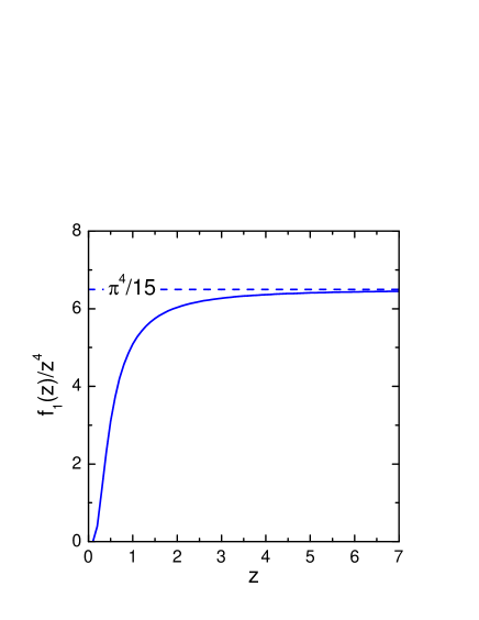
Figure 3: $f_{1}(z)/z^{4}$, cf. eq. (165). Dash line demonstrates asymptotic behavior for $z\gg 1$.

Numerical evaluation of the intensity $J_{1}^{v}$ is demonstrated in Fig. 3,

$$J_{1}^{v}=\frac{\pi^{2}g_{v}^{2}(m_{bt}^{*})^{2}z^{4}}{30\beta_{v}^{5/2}}r_{v}(z),\quad r_{v}(z)=\frac{15f_{1}(z)}{\pi^{4}z^{2}},\quad z=\frac{T}{m_{bt}^{*}}.$$ (165)

The horizontal line shows the asymptotic behavior (163), $r_{v}\rightarrow 1$ for $z\rightarrow\infty$. Comparing (163), (164) with expressions (68), (69) for the scalar boson case we see that in the high temperature limit ($T\gg m_{bt}^{*}(T)$) the intensity of the multiple scattering $J_{1}^{v}$ is much higher in the vector case (for $g_{v}\sim g_{s}$ and for $m_{bt}^{*}\sim m_{s}^{*}$). At these conditions the quantity $J_{0}^{v}$ is of the same order of magnitude as $J_{0}^{s}$. Please notice that $J_{1}^{v}\rightarrow\infty$ for $m_{bt}^{*}(T)\rightarrow 0$. Thus we deal here with a strong critical opalescence.

Replacing $G_{1}$ from the second equation (5.3.1) to the first one we obtain one differential equation

$$(p^{2}_{0}-\epsilon_{p}^{2}-3J_{0}^{v}-J_{01}^{v})G_{2}-1+2(J_{1}^{v}+J_{11}^{v})(2p^{2}_{0}-3J_{0}^{v}-J_{01}^{v})\frac{dG_{2}}{dp^{2}_{0}}$$

$$+4(J_{1}^{v}+J_{11}^{v})^{2}p_{0}^{2}\frac{d^{2}G_{2}}{(dp^{2}_{0})^{2}}=0.$$ (166)

Equation (5.3.1) can be solved perturbatively only for very small values of $J^{v}_{0}$, $J^{v}_{1}$, $J^{v}_{01}$, $J^{v}_{11}$. For typical values $p_{0}^{2}-\epsilon_{p}^{2}\ll m_{f}T$ permitted within the quasiparticle approximation, the perturbative regime would hold only for $J^{v}_{1},J^{v}_{01},J^{v}_{11}\ll T^{2}$. On the other hand, as we have mentioned, at rather low temperature the STL approximation is not applicable anymore. Even in the low temperature limit for the regime of a warm hadron liquid the quasiparticle approximation (for $g_{v}\sim 10$) and the perturbative approach fail, as we have shown it above.

5.3.2 Non-relativistic fermion distributions and blurring of the fermion continuum

In non-relativistic approximation for fermions, as we shall see it below (cf. eqs (169), (5.3.2)), typical fermion 4-momenta of our interest are given by

$$p^{2}\simeq m_{f}^{2}+O\left(\sqrt{J_{1}^{v}}\,m_{f};J_{1}^{v}m_{f}T^{-1}\right).$$ (167)

For such momenta one may drop the higher order derivative term in (5.3.1) Then eq. (5.3.1) is simplified as

$$\frac{(\gamma^{\rm n.rel}_{v})^{2}}{2}\frac{dG_{2}}{dz}+zG_{2}-1=0,\quad z\simeq p^{2}_{0}-\epsilon_{p}^{2},$$ (168)

$$(\gamma^{\rm n.rel}_{v})^{2}\simeq 8(J_{1}^{v}+J_{11}^{v})m_{f}^{2}.$$

The form of eq. (168) coincides with that have been used for the description of the blurring of the electron gap in semiconductors due to the electron-phonon interaction [6]. Heavy fermions (e.g., nucleons) play the same role, as electrons, whereas light vector bosons (e.g., $\omega$ with an effective mass $m^{*}_{\omega t}(T)\ll m_{N}$) play the role of phonons.

Solution of (168) satisfying appropriate condition $G_{2}\rightarrow 1/z$ for $z\rightarrow\infty$ ($z\gg\gamma_{v}^{\rm n.rel}$ to be more concrete) can be presented in the integral form

$$G_{2}(z)=\frac{1}{\sqrt{\pi}\gamma_{v}^{\rm n.rel}}\int^{\infty}_{-\infty}(z-\eta)^{-1}e^{-(\eta^{2}/(\gamma^{\rm n.rel}_{v})^{2})}d\eta.$$ (169)

Now we may recover the explicit expression for the full vertex $\widehat{V}^{\mu}(q=0,p,p)$. From (5.3.1) and (168) we find

$$\widehat{G}_{f}\simeq G_{2}^{f}(\hbox{$/$}\kern-5.01563pt\hbox{$p$}+m_{f})+\hbox{$/$}\kern-5.01563pt\hbox{$p$}\frac{1-zG_{2}}{2m_{f}^{2}},$$ (170)

i.e. $\widehat{G}_{f}\simeq G_{2}^{f}(\hbox{$/$}\kern-5.01563pt\hbox{$p$}+m_{f})$ for typical energies and momenta of our interest. Using (151) and (168) we obtain

$$\widehat{V}^{\mu}(q=0,p,p)\simeq-\frac{2p^{\mu}(\hbox{$/$}\kern-5.01563pt\hbox{$p$}-m_{f})[2(1-zG_{2})z+G_{2}(\gamma^{\rm n.rel}_{v})^{2}]}{(\gamma^{\rm n.rel}_{v})^{2}z^{2}G_{2}^{2}}+\frac{\gamma^{\mu}}{zG_{2}}.$$ (171)

In order to calculate fermion distributions and the density we need to know ${\rm Im}G$. From (169) and (170) we find

$${\rm Im}G_{2}=-\frac{\sqrt{\pi}}{\gamma_{v}^{\rm n.rel}}e^{-z^{2}/(\gamma^{\rm n.rel}_{v})^{2}},\quad{\rm Im}G_{1}={\rm Im}G_{2}\left(1-\frac{z}{2m_{f}^{2}}\right).$$ (172)

We see that ${\rm Im}G_{1}\simeq{\rm Im}G_{2}$ for $|z|\ll m_{f}^{2}$ of our interest. The imaginary part of the Green function given by (172) satisfies the sum rule (241) for $|z|\ll m_{f}^{2}$.

For typical energies given by eq. (167) with the help of (A.2) we obtain

$$\widehat{n}_{f,(\pm)}\simeq\frac{\gamma_{0}+1}{2\sqrt{\pi}\,\gamma_{v}^{\rm n.rel}}\mbox{exp}\left[-\frac{(\epsilon_{p}\mp\mu_{f})}{T}\right]\int_{-\infty}^{\infty}dz\mbox{exp}\left[-\left(\frac{z^{2}}{(\gamma^{\rm n.rel}_{v})^{2}}+\frac{z}{2\epsilon_{p}T}\right)\right]$$

$$\simeq\frac{\gamma_{0}+1}{2}\mbox{exp}\left[-\frac{(\epsilon_{p}\mp\mu_{f})}{T}+\frac{(\gamma^{\rm n.rel}_{v})^{2}}{16\epsilon_{p}^{2}T^{2}}\right].$$ (173)

Compare this result with (76). For $\sqrt{J_{1}^{v}+J_{11}^{v}}\ll T$ (low temperatures) eq. (5.3.2) yields only a slightly corrected Boltzmann distribution. However (5.3.2) becomes incorrect in the low temperature limit due to the violation of the STL approximation in this limit. In opposite limit case, $\sqrt{J_{1}^{v}+J_{11}^{v}}\gg T$, the 3-momentum fermion distribution is exponentially enhanced.

For the fermion-antifermion density we obtain

$$\rho_{f,(\pm)}=\rho_{{\rm Bol},(\pm)}\mbox{exp}\left(\frac{J_{1}^{v}+J_{11}^{v}}{2T^{2}}\right).$$ (174)

The value

$$m_{f}^{*}=m_{f}-\mu_{f}-\frac{J_{1}^{v}+J_{11}^{v}}{2T},$$ (175)

as it is extracted from (5.3.2), plays the role of the effective fermion mass.

The temperature $T_{\rm bl.f}^{v,{\rm n.rel}}$ is estimated from the condition $m_{f}^{*}(T_{\rm bl.f}^{v,{\rm n.rel}})=0$. Then from (175), (165) we evaluate

$$T_{\rm bl.f}^{v,{\rm n.rel}}\simeq\left[\frac{60m_{bt}^{*\,2}(m_{f}-\mu_{f})}{\pi^{2}g_{v}^{2}r_{v}(T_{\rm bl.f}^{v,{\rm n.rel}})}\right]^{1/3}.$$ (176)

Simplifying, we suppressed the contribution $J_{11}^{v}$ in this estimate. Comparing (176) with (85) for scalar bosons for $r_{v}\simeq r_{s}\simeq 1$ we see that in the heavy fermion limit ($m_{f}\gg m_{b}^{*}$) and for $g_{s}\sim g_{v}$ we have $T_{\rm bl.f}^{v,{\rm n.rel}}<T_{\rm bl.f}^{s,{\rm n.rel}}$, i.e. in this limit vector bosons contribute more in the blurring of the fermion continuum than scalar bosons. Please notice that deriving eq. (176) we assumed $A_{b,(\pm)}^{t}\simeq A_{b,(\pm)}^{l}$. The latter condition is not fulfilled for $m_{bt}^{*}\ll m_{b}$. Thus (176) can be considered only as a rough estimate.

For the $\omega$ meson from (176) we would obtain $T_{\rm bl.f}^{v,0,{\rm n.rel}}\simeq 2.3m_{\pi}$, for $g_{\omega}=10$, $r_{v}\simeq 1$ and for the mass $m_{bt}^{*}=m_{\omega}=782$ MeV. But then $T_{\rm bl.f}^{v,0,{\rm n.rel}}\ll m_{bt}^{*}(T_{\rm bl.f}^{v,0,{\rm n.rel}})$ and the condition for the use of the high temperature limit is violated ($r_{v}\ll 1$). By index zero we again indicate that we will refuse of this estimate. Thus one should take into account the decrease of $m_{\omega t}^{*}$ for $T\sim T_{\rm bl.f}^{v,{\rm n.rel}}$. Taking $m_{bt}^{*}\simeq m_{\pi}$ we would get $T_{\rm bl.f}^{v,{\rm n.rel}}\simeq 120~{}$MeV. However, as we have demonstrated in case of the $\sigma$ meson, fully correct estimate should be done within self-consistent account of both the fermion and the boson coupled channels. Finally we may roughly evaluate $T_{\rm bl.f}^{v,{\rm n.rel}}\stackrel{{\scriptstyle\scriptstyle<}}{{\phantom{}{}_{\sim}}}m_{\pi}$.

We supplied the value $T_{\rm bl.f}^{v,{\rm n.rel}}$ with the index ${}^{\prime\prime}{\rm n.rel}^{\prime\prime}$, since the estimate was done in the non-relativistic approximation for fermions. In pure relativistic case one needs to solve much more involved eq. (5.3.1). Without additional calculations we may only conclude that for relativistic fermions the value $T_{\rm bl.f}^{v}$ is still less than $T_{\rm bl.f}^{v,{\rm n.rel}}$. However in our model example we did not take into account interaction with other mesons, e.g. scalar boson correlation terms. Such terms suppress vertices that may result in an increase of the actual value of $T_{\rm bl.f}^{v}$.

5.3.3 Vector-isospin vector boson – fermion system

The vector-isospin vector boson – fermion system (the interaction term $L_{int}=-g_{i.v}\bar{\psi}\gamma_{\mu}\vec{\tau}\vec{\phi}^{\mu}\psi$) is considered in the same manner, as the vector boson – fermion system just discussed. All expressions obtained for vector bosons continue to hold also for vector-isospin vector bosons, if one replaces $g_{v}\rightarrow g_{v}^{*}\simeq\sqrt{3}g_{i.v.}$.

For $\omega$ and $\rho$ mesons one has $g_{\omega}\simeq 8\div 10$ and $g_{\rho}\simeq 2.5\div 3$, from where we estimate that the effective $\rho$ meson coupling is $\sim 0.5$ of that for the $\omega$.

5.3.4 Comparison with example of one diagram of $\Phi$ (no correlations)

To compare our general result with the result one would obtain without inclusion of correlations let us consider the problem with only one diagram of $\Phi$ (first diagram (2)). In this case one should replace the vertex (151) by the bare vertex $\gamma^{\mu}$. In the STL approximation the Dyson equation (152) then takes the form

$$\widehat{G}_{f}^{R}=\widehat{G}_{f}^{0,R}-\widehat{G}_{f}^{0,R}J_{v}^{\mu\nu}\gamma_{\mu}\widehat{G}_{f}^{R}\gamma_{\nu}\widehat{G}_{f}^{R},$$ (177)

with $J_{v}^{\mu\nu}$ given by eq. (154). Again, to simplify the consideration we will assume that $A_{b,(\pm)}^{t}\simeq A_{b,(\pm)}^{l}$, being correct in the case of a small change of the effective vector boson mass. This assumption allows us to omit values $J_{01}^{v}$ and $J_{11}^{v}$.

Now we may work out the tensor structure of (177). For that we first calculate the auxiliary quantity

$$(\delta_{\mu}^{\nu}-\frac{q_{\mu}q^{\nu}}{q^{2}})\gamma^{\mu}(G_{1}\hbox{$/$}\kern-5.01563pt\hbox{$p$}+G_{2}m_{f})\gamma_{\nu}(G_{1}\hbox{$/$}\kern-5.01563pt\hbox{$p$}+G_{2}m_{f})$$ (178)

$$=-G_{1}^{2}p^{2}+2m_{f}\hbox{$/$}\kern-5.01563pt\hbox{$p$}G_{1}G_{2}+3m_{f}^{2}G_{2}^{2}-2\frac{(pq)\hbox{$/$}\kern-4.91145pt\hbox{$q$}\hbox{$/$}\kern-5.01563pt\hbox{$p$}}{q^{2}}G_{1}^{2}-2m_{f}\frac{\hbox{$/$}\kern-4.91145pt\hbox{$q$}(pq)}{q^{2}}G_{1}G_{2},$$

see eq. (157).

Let us again use the non-relativistic approximation for fermions. Then we may suppress terms containing $\vec{p}\,\vec{q}$ compared to the corresponding term $\propto p_{0}q_{0}\sim m_{f}q_{0}$. Also we drop the term $\propto\vec{\gamma}$, which does not contribute to the particle density. Then we obtain two coupled equations

$$p^{2}G_{1}-m_{f}^{2}G_{2} = 1+J_{0}^{v}(G_{1}^{2}p^{2}-3G_{2}^{2}m_{f}^{2})+2J^{v}_{2}m_{f}^{2}G_{1}^{2},$$

$$G_{2}-G_{1} = 2J^{v}_{1}G_{1}G_{2},$$ (179)

with

$$J_{2}^{v}=g_{v}^{2}\int\frac{q_{0}^{2}}{q^{2}}\frac{d^{3}q}{(2\pi)^{3}}\int_{0}^{\infty}\frac{dq_{0}}{2\pi}\left[A_{b,(+)}^{t}n_{b,(+)}(q_{0})+A_{b,(-)}^{t}n_{b,(-)}(q_{0})\right].$$ (180)

Within the quasiparticle approximation for bosons $J_{2}^{v}$ is expressed through $J_{0}^{v}$ and $J_{1}^{v}$.

We replace $G_{1}$ from the second eq. (5.3.4) to the first one and retain there only quadratic terms in $G_{2}$, where we put $p^{2}\simeq m_{f}^{2}$, and we use $J^{v}_{1}\ll m_{f}^{2}$. Approximations are correct for typical momenta of our interest given by (167). Then we find

$$G_{2}^{R}\simeq\frac{p^{2}-m_{f}^{2}\pm i\sqrt{2(\gamma^{{\rm n.rel}}_{v})^{2}-(p^{2}-m_{f}^{2}+i0)^{2}}}{(\gamma^{{\rm n.rel}}_{v})^{2}}.$$ (181)

For $|p^{2}-m_{f}^{2}|<\sqrt{2}\gamma^{{\rm n.rel}}_{v}$ the upper sign solution should be dropped. This result is nicely matched with that in the scalar case, cf. (4.2.3). The difference is only in the value of the intensity of the multiple scattering ($J_{1}^{v}$ in the vector boson case instead of $J_{s}$ in the scalar boson case). Imaginary part of the Green function (181) satisfies the exact sum rule. However we note that the Green function (181) is quite different from that given by eqs (169), (172), which exploit the full vertex.

We conclude that in the vector boson case correlations qualitatively change the picture modifying expressions for the effective fermion mass and the value of the temperature $T_{\rm bl.f}^{v}$.

5.4 Hot vector boson condensation

Now let us consider a possibility of the HBC for vector bosons. To simplify the consideration we will not discuss a modification of the vector boson spectrum rather we will only estimate the critical temperature for the HBC in the transversal channel. For that we need only to evaluate the quantity ${\rm Re}(\Sigma_{b})^{i}_{i}(q_{0}=0,|\vec{q}|\rightarrow 0)$, cf. (5.1).

Using (16), where we replace one bare vertex to the full vertex (151), we obtain

$${\rm Re}(\widehat{\Sigma}_{b}^{R})^{\nu\mu}(q_{0}=0,|\vec{q}|\rightarrow 0)\simeq-4g_{v}^{2}\mbox{Tr}\int\frac{d^{3}p}{(2\pi)^{3}}\int_{0}^{\infty}\frac{dp_{0}}{2\pi}\gamma^{\nu}{\rm Re}\widehat{G}_{f}^{R}(p)$$ (182)

$$\times {\rm Re}\frac{\partial\widehat{G}_{f}^{-1}}{\partial p_{\mu}}{\rm Im}\widehat{G}_{f}^{R}(p)n_{f}(p_{0})+\{f\rightarrow\bar{f}\}.$$

With the help of eq. (171), where only second term contributes, assuming $G_{1}\simeq G_{2}$ (non-relativistic nucleons) we find

$${\rm Re}(\widehat{\Sigma}_{b}^{R})^{i}_{i}(q_{0}=0,|\vec{q}|\rightarrow 0)\simeq 48g_{v}^{2}\int\frac{d^{3}p}{(2\pi)^{3}}\int_{0}^{\infty}\frac{dp_{0}}{2\pi}$$

$$\times{\rm Im}G_{2}n_{f}(p_{0})+\{f\rightarrow\bar{f}\}.$$ (183)

Using (A.2), (248) and (5.1) we obtain

$${\rm Re}(\Sigma_{b}^{R})^{t}(q_{0}=0,|\vec{q}|\rightarrow 0)\simeq-6g_{v}^{2}\rho_{f,\bar{f}}/m_{f}.$$ (184)

Here $\rho_{f,\bar{f}}$ is, as before, the density of fermion-antifermion pairs of one fermion species. In reality other fermion species (e.g., as neutrons and protons) may also contribute to $\widehat{\Sigma}_{b}$.

The critical temperature and the fermion-antifermion density for the HBC of vector bosons in the transversal channel under consideration would be found from the condition

$$m_{bt}^{*\,2}=m_{b}^{2}+{\rm Re}(\Sigma_{b}^{R})_{tr}(q_{0}=0,|\vec{q}|\rightarrow 0)=0,$$ (185)

if it had the solution. However, since the intensity of the multiple scattering $J_{1}^{v}$ tends to infinity for $m_{bt}^{*\,2}\rightarrow 0$, see (163), the density of fermion-antifermion pairs given by eq. (174) is anomalously increased. This motivates the possibility of the first order phase transition to the HBC state with a jump of $m_{bt}^{*\,2}(T_{\rm cb}^{v})$ from a positive to a negative value in the critical point.

Let us assume that this jump occurs at $m_{bt}^{*\,2}=\zeta m_{bt}^{2}$, $0<\zeta<1$. Then with the help of eq. (184) we find

$$\rho_{f,\bar{f}}^{\rm cb}(T_{\rm cb}^{v})\simeq\frac{m_{f}m_{b}^{2}(1-\zeta)}{6g_{v}^{2}}.$$ (186)

Note that eq. (174) was derived in the non-relativistic approximation for fermions. It should be replaced to the relativistic expression at temperatures, when $m_{f}^{*}(T)$ becomes to be $\stackrel{{\scriptstyle\scriptstyle<}}{{\phantom{}{}_{\sim}}}T$. Thus eq. (186) yields a correct estimate only, if $m_{f}^{*}(T)\stackrel{{\scriptstyle\scriptstyle>}}{{\phantom{}{}_{\sim}}}T$. To further study the first order phase transition one needs to calculate the contribution to the thermodynamic potential in both phases. This requires a more detailed analysis. Only for a rough estimate of the value $T_{\rm cb}^{v}$ one may use (174), (163), (186).

If the system consists of two fermion species (e.g., neutrons and protons) it can be taken into account by the replacement $\rho_{f,\bar{f}}^{\rm cb}\rightarrow 2\rho_{f,\bar{f}}^{\rm cb}=\rho_{N,\bar{N}}^{\rm cb}$ in the boson self-energy. For the $N\bar{N}\omega$ (two fermion species) and for $g_{v}\simeq 10$, $m_{\omega}\simeq 782~{}$MeV, $m_{N}\simeq 933~{}$MeV, assuming $m_{bt}^{*}(T_{\rm cb}^{v})\simeq m_{\pi}$ we estimate $\rho_{N,\bar{N}}^{\rm cb}\simeq 0.7\rho_{0}$. According to (174) and (165), the density $\rho_{N,\bar{N}}^{\rm cb}\simeq 0.7\rho_{0}$ corresponds to the temperature $T\simeq 110~{}$MeV. The value $0.7\rho_{0}$ at such a low temperature is well below the deconfinement density. Thus quark effects seem to be still unimportant. However note that values $T_{\rm bl.f}^{\rm v,n.rel}\simeq 120~{}$MeV and $T_{\rm cb}^{v}\simeq 110~{}$MeV could be underestimations, as the result of crude approximations, which we have done. As we have mentioned the non-relativistic limit eq. (174) might become quantitatively incorrect in the vicinity of $T_{\rm bl.f}^{\rm v,n.rel}$ yielding an overestimation of the density and, thus, an underestimation of $T_{\rm cb}^{v}$. Another reason might be that in reality $g_{v}$ is less than $10$. For $g_{v}\simeq 8$ we would get higher values $T_{\rm bl.f}^{\rm v,n.rel}\simeq 140~{}$MeV, $T_{\rm cb}^{v}\simeq 130~{}$MeV. Nevertheless, within a reasonable variation of parameters we always obtain that the blurring of the nucleon continuum and the HBC of $\omega$ and $\rho$ mesons could occur already for $T<m_{\pi}$. Concluding this discussion we again stress that we considered a model problem and disregarded many relevant couplings that might yield an effective repulsion.

The typical behavior of the logarithm of the ratio of the fermion density to the corresponding Boltzmann quantity as function of the temperature is shown in Fig. 4 for $T<T_{\rm cb}^{v}$. Moreover Fig. 4 demonstrates the temperature dependence of the effective transverse vector boson mass. We see a huge enhancement of $\mbox{ln}(\rho_{f}/\rho_{f,\rm Bol})$ and a drastic decrease of $m_{bt}^{*}/m_{b}$ in the vicinity of $T=T_{\rm bl.f}^{v},T_{\rm cb}^{v}$. At the critical point the first order phase transition to the HBC state may occur. The value $m_{bt}^{*}/m_{b}$ does not reach zero at this point.

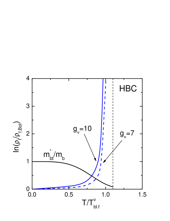
Figure 4: Logarithm of the ratio of the fermion density to the corresponding Boltzmann quantity for $g_{v}=10$ and $g_{v}=7$, and the effective transverse vector boson mass as functions of the temperature in units of $T_{\rm bl.f}^{v}$. The vertical dash-line indicates the area of the HBC.

6 Heavy fermions and less massive pseudo-scalar bosons (pseudo-vector coupling)

Let us now consider pseudo-scalar boson – spin $\frac{1}{2}$ fermion system interacting via the pseudo-vector coupling

$$L_{int}=-ig_{p.v}m_{b}^{-1}\bar{\psi}\widehat{q}\gamma_{5}\vec{\tau}\vec{\phi}\psi.$$ (187)

In realistic case bosons are $\pi^{+},\pi^{-},\pi^{0}$ and fermions are $n$ and $p$. The $\pi NN$ coupling is $g_{p.v}\simeq 1$.

6.1 Low temperature limit

Again we start with the simplest $\Phi$ given by the first diagram (2). We calculate the value

$$\widehat{S}^{0}=\widehat{V}_{0}(q)\widehat{\Lambda}_{f}^{0}(p+q)\widehat{V}_{0}(-q)\widehat{\Lambda}_{b}^{0}(q)$$

$$=N_{p.v}g_{p.v}^{2}m_{b}^{-2}[2pq\hbox{$/$}\kern-4.91145pt\hbox{$q$}-(m_{f}+\hbox{$/$}\kern-5.01563pt\hbox{$p$})q^{2}+q^{2}\hbox{$/$}\kern-4.91145pt\hbox{$q$}],$$ (188)

where $N_{p.v}=3$ is the isospin degeneracy factor ($\pi^{+},\pi^{-},\pi^{0}$). Within the non-relativistic approximation for fermions replacing $p_{0}\simeq m_{f}$, $q^{2}\simeq m_{b}^{2}$, using $q_{0}\ll m_{f}$, $|\vec{q}|\ll m_{f}$, and retaining only zero components of vectors (dropping linear terms in $\vec{\gamma}$, which do not further contribute) we simplify (6.1) as follows

$$\widehat{S}^{0}\simeq N_{p.v}g_{p.v}^{2}m_{b}^{-2}m_{f}\left[\vec{q}^{\,2}(1+\gamma_{0})-q_{0}^{2}(1-\gamma_{0})\right].$$ (189)

With the help of eqs (189), (24), (26) we calculate the fermion 3-momentum distribution

$$\widehat{n}_{f,(\pm)}(\vec{p})\simeq\left[\frac{(\epsilon_{p}+m_{f}\gamma_{0})}{2\epsilon_{p}}+\frac{(1+\gamma_{0})N_{p.v}g_{p.v}^{2}}{8\pi^{2}}I_{0v}^{0}(\frac{\epsilon_{p}}{m_{b}})\right]n_{{\rm Bol},(\pm)},$$ (190)

where $I_{0v}^{0}(x)$ is determined by eq. (143).

Finally, the fermion particle and antiparticle densities are

$$\frac{\rho_{f,(+)}}{\rho_{{\rm Bol},(+)}}=\frac{\rho_{f,(-)}}{\rho_{{\rm Bol},(-)}}\simeq 1+\frac{N_{p.v}g_{p.v}^{2}}{4\pi^{2}}I_{0v}^{0}\left(\frac{m_{f}}{m_{b}}\right).$$ (191)

This result essentially differs from eq. (49) for scalar neutral bosons, since $I_{0v}^{0}$ and $I_{0s}$ are different. The difference with the result for the vector-isospin vector boson system for the case of a warm hadron liquid, where $I_{0v}^{1}$ term is suppressed (see eq. (147)), is hidden in the different coupling constants and spin-isospin dependent coefficients.

For $T\sim m_{\pi}/2$, the regime of the warm hadron liquid is realized, $m_{b}\gg T\gg m_{b}^{2}/m_{f}$. We find $\rho_{p}^{sym}=\rho_{n}^{sym}=\rho_{\bar{p}}^{sym}=\rho_{\bar{n}}^{sym}\simeq 1.16\rho_{\rm Bol}^{sym}$, that yields rather small correction due to a moderate value of the coupling constant, $g_{\pi N}\simeq 1\ll g_{\sigma N}\simeq 10$. Nevertheless this correction is of the order of that for $\sigma$ and $\omega$ mesons. The reason is that the pion is lighter than $\sigma$ and $\omega$. Thereby, $I_{0v}^{0}$ is enhanced, see eq. (145). Moreover for $T\sim m_{\pi}/2$ for $\sigma$ and $\omega$ still the regime of the slightly heated hadron liquid occurs rather than the regime of the warm hadron liquid, as for the pion.

Contribution of the correlation diagrams is negligible in the low temperature limit, as in the scalar and vector boson cases.

6.2 High temperature limit

6.2.1 Analytic solution for fermion Green functions in STL approximation

We continue operate with the single diagram of $\Phi$ (the first diagram (2)). Now we calculate the value

$$\widehat{S}=\widehat{V}_{0}(q)\widehat{\Lambda}_{f}(p)\widehat{V}_{0}(-q)\widehat{\Lambda}_{b}^{0}(q)\widehat{\Lambda}_{f}(p)$$

$$=3g_{p.v}^{2}m_{b}^{-2}\left(-p^{2}q^{2}+2(pq)\hbox{$/$}\kern-4.91145pt\hbox{$q$}\hbox{$/$}\kern-5.01563pt\hbox{$p$}\right)(G_{1}^{R})^{2}$$

$$-3g_{p.v}^{2}m_{b}^{-2}\left(m_{f}^{2}q^{2}(G_{2}^{R})^{2}+2m_{f}(q^{2}\hbox{$/$}\kern-5.01563pt\hbox{$p$}-qp\cdot\hbox{$/$}\kern-4.91145pt\hbox{$q$})G_{1}^{R}G_{2}^{R}\right),$$ (192)

entering eq. (31). We used eq. (37), where we have put $G_{3}=0$. Dropping terms linear in $\vec{\gamma}$ and $\vec{q}\vec{p}$ and using (37), we may rewrite the Dyson equation (34) for the fermion sub-system, as the system of coupled equations

$$p^{2}G_{1}^{R}-m_{f}^{2}G_{2}^{R}=1+[(J_{1}^{p.v}-J_{2}^{p.v})p^{2}+2p_{0}^{2}J_{2}^{p.v}](G_{1}^{R})^{2}$$

$$+(J_{1}^{p.v}-J_{2}^{p.v})m_{f}^{2}(G_{2}^{R})^{2},$$

$$G_{2}^{R}=G_{1}^{R}+2J_{1}^{p.v}G_{1}^{R}G_{2}^{R},$$ (193)

where now

$$J^{p.v}_{1}=\frac{3g_{p.v.}^{2}}{m_{b}^{2}}\int\frac{\vec{q}^{\,\,2}d^{3}q}{(2\pi)^{3}}\int_{0}^{\infty}\frac{dq_{0}}{2\pi}\left[\widehat{A}_{b,(+)}n_{b,(+)}(q_{0})+\widehat{A}_{b,(-)}n_{b,(-)}(q_{0})\right],$$ (194)

$$J^{p.v}_{2}=\frac{3g_{p.v.}^{2}}{m_{b}^{2}}\int\frac{q^{\,\,2}_{0}d^{3}q}{(2\pi)^{3}}\int_{0}^{\infty}\frac{dq_{0}}{2\pi}\left[\widehat{A}_{b,(+)}n_{b,(+)}(q_{0})+\widehat{A}_{b,(-)}n_{b,(-)}(q_{0})\right].$$ (195)

Setting $G_{1}\simeq G_{2}$ in quadratic terms ($(G^{R})^{2}$) we arrive at the Dyson equation

$$G_{1}^{R}=G_{f}^{0,R}+G_{f}^{0,R}[(p_{0}^{2}+3m_{f}^{2})J^{p.v}_{1}-(J^{p.v}_{1}-J^{p.v}_{2})\vec{p}^{\,2}](G_{1}^{R})^{2}$$

$$+J^{p.v}_{2}(G_{1}^{R})^{2}.$$ (196)

This equation already allows for the analytic solution.

6.2.2 Intensity of multiple scattering

Within the quasiparticle approximation for bosons and antibosons the spectrum of boson excitations becomes

$$\omega_{(\pm)}^{2}(\vec{q},T) \simeq m_{b}^{2}+\beta_{p.v}(T)\vec{q}^{\,2}+\widetilde{\beta}_{p.v}(T)\vec{q}^{\,4}+...,$$

cf. subsection 6.3. Due to the p-wave nature of the interaction (187) in eq. (6.2.2) there appear the bare boson mass and a significantly corrected $\vec{q}^{\,2}$ term. Even one may have $\beta_{p.v}<0$ in some temperature interval. For cases of sufficiently small $\beta_{p.v}$ and for $\beta_{p.v}<0$ one should keep in (6.2.2) the higher order terms, at least the $\vec{q}^{\,4}$ term.

Using this spectrum we may evaluate the intensity of the multiple scattering $J^{p.v}_{1}$. For $\beta_{p.v}>0$, assuming it is not as small, dropping the term $\widetilde{\beta}_{p.v}\vec{q}^{\,4}$ in (6.2.2), with the help of eq. (194) we find

$$J^{p.v}_{1} = \frac{6g_{p.v}^{2}}{m_{b}^{2}}\int\frac{\vec{q}^{\,\,2}d^{3}q}{(2\pi)^{3}}\int_{0}^{\infty}\frac{dq_{0}\delta\left(q_{0}^{2}-m_{b}^{2}-\vec{q}^{\,\,2}-{\rm Re}\Sigma_{b}^{R,(0)}(q^{2})\right)}{e^{q_{0}/T}-1}$$

$$= \frac{3g_{p.v}^{2}}{2\pi^{2}m_{b}^{2}}\int_{0}^{\infty}\frac{\vec{q}^{\,\,4}d|\vec{q}|}{\left(m_{b}^{2}+\beta_{p.v}\vec{q}^{\,\,2}\right)^{1/2}}\frac{1}{\mbox{exp}\left[\left(m_{b}^{2}+\beta_{p.v}\vec{q}^{\,\,2}\right)^{1/2}/T\right]-1},$$

and in limiting cases

$$J^{p.v}_{1} = \frac{\pi^{2}g_{p.v}^{2}T^{4}}{10\beta_{p.v}^{5/2}m_{b}^{2}}\,,\quad\mbox{for}\quad T\gg m_{b},$$ (199)

$$J^{p.v}_{1} = \frac{9g_{p.v}^{2}T^{5/2}}{2^{3/2}\pi^{3/2}\beta_{p.v}^{5/2}m_{b}^{1/2}}\mbox{exp}\left(-m_{b}/T\right)\,,\quad\mbox{for}\quad T\ll m_{b}.$$ (200)

Compare these expressions with the corresponding eqs (163), (164) for the vector boson case.

Using (195) we obtain (for $\beta_{p.v}>0$)

$$J^{p.v}_{2} = \frac{3g_{p.v}^{2}}{2\pi^{2}m_{b}}\int_{0}^{\infty}\frac{\vec{q}^{\,\,2}d|\vec{q}|\left(m_{b}^{2}+\beta_{p.v}\vec{q}^{\,\,2}\right)^{1/2}}{\mbox{exp}\left[\left(m_{b}^{2}+\beta_{p.v}\vec{q}^{\,\,2}\right)^{1/2}/T\right]-1},$$ (201)

and in limiting cases

$$J^{p.v}_{2} = \frac{\pi^{2}g_{p.v}^{2}T^{4}}{10\beta_{p.v}^{3/2}m_{b}^{2}}\,,\quad\mbox{for}\quad T\gg m_{b},$$ (202)

$$J^{p.v}_{2} = \frac{3g_{p.v}^{2}T^{3/2}m_{b}^{1/2}}{2^{3/2}\pi^{3/2}\beta_{p.v}^{3/2}}\mbox{exp}\left(-m_{b}/T\right)\,,\quad\mbox{for}\quad T\ll m_{b}.$$ (203)

For $\beta_{p.v}\rightarrow 0$ intensities of the multiple scattering anomalously increase. However in reality they do not tend to infinity, if one incorporated the term $\widetilde{\beta}_{p.v}\vec{q}^{\,\,4}$ in eq. (6.2.2).

The maximum value of the density that can be achieved in this regime can be estimated as (86), now using eq. (202):

$$\rho_{f,(\pm)}^{\rm max}\simeq\frac{m_{f}^{3/2}T^{3}}{2^{3/2}\pi^{2}J_{s}^{3/4}}\rightarrow\frac{5^{3/4}\beta_{p.v}^{9/8}m_{f}^{3/2}m_{b}^{3/2}}{2^{3/4}\pi^{7/2}g_{p.v}^{3/2}}.$$ (204)

As we shall see in subsection 6.3, the quantity $\beta_{p.v}$ decreases with the increase of the temperature. For $T=T_{{\rm cb},1}^{p.v}$ the value $\beta_{p.v}$ reaches zero and for $T>T_{{\rm cb},1}^{p.v}$ it becomes negative. In refs [26, 33] the density/temperature, when $\beta_{p.v}$ crosses zero, was called the critical density/temperature for the appearance of the liquid phase of the pion condensation. There is no yet a long-ranged order for $T_{\rm cb}^{p.v}>T>T_{{\rm cb},1}^{p.v}$. However there arise many virtual boson excitations carrying finite momentum $|\vec{q}_{c}|$. Actual values of particle momenta are near $|\vec{q}_{c}|$, and directions of the momenta are randomly distributed. For $\beta_{p.v}(T)<0$, the quantity

$$\widetilde{\omega}^{2}(\vec{q},T)=m_{b}^{2}+{\rm Re}\Sigma_{b}^{R}(q_{0}=0,\vec{q},T),$$ (205)

that can be called the effective boson gap, gets the minimum, cf. [14, 33]. At low $q_{0}$, the boson spectrum has a non-quasiparticle nature. As we will demonstrate it below, see eqs (6.3), (226), the dispersion relation is then given by

$$i\beta_{1}(|\vec{q}|)\omega\simeq\omega_{0}^{2}+\beta_{0}(|\vec{q}|-|\vec{q}_{c}|)^{2},\quad|\vec{q}_{c}|\neq 0,\,\omega_{0}^{2},\,\beta_{1},\,\beta_{0}>0,$$ (206)

where

$$\omega_{0}^{2} = \widetilde{\omega}^{2}(\vec{q}_{c})=m_{b}^{2}+{\rm Re}\Sigma_{b}^{R}(q_{0}=0,\vec{q}=\vec{q}_{c})$$

$$\simeq m_{b}^{2}-\beta_{p.v}^{2}/(4\widetilde{\beta}_{p.v}).$$

The value

$$|\vec{q}_{c}|\simeq\sqrt{-\beta_{p.v}/(2\widetilde{\beta}_{p.v})}$$ (208)

corresponds to the minimum of $\widetilde{\omega}^{2}(|\vec{q}|)$, $\beta_{0}\simeq-2\beta_{p.v}$. The form of the spectrum (206) coincides with that previously used in the description of the dense baryon matter in the pion condensation problem, cf. [14]. The boson spectral function has the form

$$\widehat{A}_{b,(\pm)}\simeq\frac{2\beta_{1}q_{0}}{[\omega_{0}^{2}+\beta_{0}(|\vec{q}|-|\vec{q}_{c}|)^{2}]^{2}+\beta_{1}^{2}q_{0}^{2}}.$$ (209)

Replacing (209) in eqs (194), (195) and using for simplicity the limit $\beta_{1}T\gg\omega_{0}^{2}$, $\beta_{1}\equiv\beta_{1}(\vec{q}_{c})$, we calculate

$$J^{p.v}_{1}\simeq\frac{3g_{p.v}^{2}\vec{q}_{c}^{\,4}T}{2\pi m_{b}^{2}\sqrt{\beta_{0}}\omega_{0}},\quad J^{p.v}_{2}\ll J^{p.v}_{1}.$$ (210)

One has $J^{p.v}_{2}\ll J^{p.v}_{1}$, since $J^{p.v}_{2}$ has no singularity for $\omega_{0}\rightarrow 0$. We find an anomalous increase of the intensity of multiple scattering for $\omega_{0}\rightarrow 0$, i.e. the critical opalescence. In the given case, as for vector bosons, it is the precursor of the first order phase transition to the HBC. However in difference with the vector boson case here the phase transition may occur to the crystalline or liquid crystalline state, see further discussion in subsection 6.3.

6.2.3 Non-relativistic fermions

In non-relativistic approximation for fermions we may put $|\vec{p}|\ll p_{0}$ and $p_{0}\simeq m_{f}$. Then (6.2.1) simplifies as

$$G_{1}^{R}=G_{f}^{0,R}+G_{f}^{0,R}4m_{f}^{2}J^{p.v}_{1}(G_{1}^{R})^{2}.$$ (211)

Its solution takes the form

$${\rm Re}G_{1}^{R}\simeq{\rm Re}G_{2}^{R}\simeq\frac{p^{2}-m_{f}^{2}}{\gamma_{p.v}^{2}},\quad\gamma_{p.v}^{2}=8J_{1}^{p.v}m_{f}^{2},$$

$${\rm Im}G_{1}^{R}\simeq{\rm Im}G_{2}^{R}\simeq-\frac{\sqrt{2\gamma_{p.v}^{2}-(p^{2}-m_{f}^{2}+i0)^{2}}}{\gamma_{p.v}^{2}},$$ (212)

for $2\gamma_{p.v}^{2}>(p^{2}-m_{f}^{2})^{2}$. The only difference with eq. (4.2.3) (the latter equation is valid for the scalar boson) is that in (6.2.3) enters $\gamma_{p.v}$ instead of $\gamma_{s}$. Therefore, after the replacement $J_{s}\rightarrow J^{p.v}_{1}$ expressions (75) – (85) hold also in the pseudo-scalar case.

The temperature of the blurring of the fermion continuum evaluated within the non-relativistic approximation for fermions ($T_{\rm bl.f}^{p.v,\rm n.rel}$) follows from the relation $J^{p.v}_{1}=m_{f}^{2}/4$ (for $\mu_{f}=0$), from where using (199) (at the condition $\beta_{p.v}>0$) we estimate, cf. [5],

$$T_{\rm bl.f}^{p.v,\rm n.rel}=\frac{5^{1/4}\beta_{p.v}^{5/8}(m_{f}m_{b})^{1/2}}{2^{1/4}\pi^{1/2}g_{p.v.}^{1/2}}.$$ (213)

6.2.4 Relativistic fermions

Let us consider the contribution of the energy region $p_{0}\ll m_{f}$. Then from (248), (4.2.4), (6.2.1) we find the fermion-antifermion density (for one species of fermion):

$$\delta\rho_{f,(\pm)}(p_{0}\stackrel{{\scriptstyle\scriptstyle<}}{{\phantom{}{}_{\sim}}}T)=\frac{T^{2}}{6\pi}\int_{0}^{|\vec{p}_{\rm max}|}\vec{p}^{\,2}d|\vec{p}|$$

$$\times\frac{\sqrt{12m_{f}^{2}J_{1}^{p.v}-4J_{1}^{p.v}\vec{p}^{\,2}-4J_{2}^{p.v}m_{f}^{2}-(\vec{p}^{\,2}+m_{f}^{2})^{2}}}{2m_{f}^{2}[3J_{1}^{p.v}-J_{2}^{p.v}-J_{1}^{p.v}\vec{p}^{\,2}/m_{f}^{2}]},$$ (214)

$$\vec{p}_{\rm max}^{\,2}=-m_{f}^{2}-2J_{1}^{p.v}+\sqrt{4(J_{1}^{p.v})^{2}+16J_{1}^{p.v}m_{f}^{2}-4J_{2}^{p.v}m_{f}^{2}},$$

cf. (91). We see that for $J_{1}^{p.v}-\frac{1}{3}J_{2}^{p.v}>J_{p.v}^{\rm bl.f}=\frac{m_{f}^{2}}{12}$ (positive square root in (6.2.4) for $\vec{p}\simeq 0$) the fermion sub-system represents a rather dense packing of fermion-antifermion pairs. The condition

$$J_{p.v}\equiv J_{1}^{p.v}-\frac{1}{3}J_{2}^{p.v}=J_{p.v}^{\rm bl.f}=m_{f}^{2}/12$$ (215)

determines the typical temperature $T_{\rm bl.f}^{p.v}$ of the blurring of the fermion continuum. Assuming $\beta_{p.v}>0$, and using (215) and high temperature limit estimates (199) and (202), we obtain

$$(J_{1}^{p.v})^{\rm bl.f}\simeq\frac{m_{f}^{2}}{4(3-\beta_{p.v})},\quad$$ (216)

and

$$T_{\rm bl.f}^{p.v}=\frac{T_{\rm bl.f}^{p.v,\rm non.rel}}{(3-\beta_{p.v})^{1/4}}=\frac{5^{1/4}(m_{f}m_{b})^{1/2}\beta_{p.v}^{5/8}}{2^{1/4}\pi^{1/2}g_{p.v.}^{1/2}(3-\beta_{p.v})^{1/4}}.$$ (217)

For pions we find $T_{\rm bl.f}^{p.v}\simeq 215$ MeV for $\beta_{p.v}=1$. As a more realistic estimation, taking $\beta_{p.v}\simeq 0.5$ we obtain $T_{\rm bl.f}^{p.v}\simeq 132$ MeV.

For $T\geq T_{\rm bl.f}^{p.v}$, small energies $p_{0}\stackrel{{\scriptstyle\scriptstyle<}}{{\phantom{}{}_{\sim}}}T$ essentially contribute to the filling of the particle and antiparticle Fermi seas. For $T$ in the vicinity of $T^{p.v}_{\rm bl.f}$, using that $|\vec{p}_{\rm max}|=0$ for $J_{p.v}=J_{p.v}^{\rm bl.f}$ and expanding $|\vec{p}_{\rm max}|$ in $0<J_{p.v}-J_{p.v}^{\rm bl.f}\ll J_{p.v}^{\rm bl.f}$, from (6.2.4) we obtain

$$|\vec{p}_{\rm max}|\simeq\frac{(36-26\beta_{p.v}+4\beta_{p.v}^{2})^{1/2}}{(7-\beta_{p.v})^{1/2}}\sqrt{J^{p.v}_{1}-(J^{p.v}_{1})^{\rm bl.f}},$$ (218)

and

$$\delta\rho_{f,,(\pm)}(p_{0}\stackrel{{\scriptstyle\scriptstyle<}}{{\phantom{}{}_{\sim}}}T)\simeq\frac{(3-\beta_{p.v})^{7/2}T^{2}\left[J_{1}^{p.v}-(J_{1}^{p.v})^{\rm bl.f}\right]^{2}}{3(7-2\beta_{p.v})^{3/2}m_{f}^{3}}\,.$$ (219)

For artificially large values $J_{1}^{p.v},J_{2}^{p.v}\gg m_{f}^{2}$ from (6.2.4) we evaluate

$$\rho_{f,(\pm)}(p_{0}\stackrel{{\scriptstyle\scriptstyle<}}{{\phantom{}{}_{\sim}}}T)\simeq\frac{T^{2}m_{f}^{2}(3-\beta_{p.v})}{24(J_{1}^{p.v})^{1/2}},\quad\vec{p}_{\rm max}^{\,2}\simeq(3-\beta_{p.v})m_{f}^{2}.$$ (220)

Using (199) we find

$$\rho_{f,(\pm)}(p_{0}\stackrel{{\scriptstyle\scriptstyle<}}{{\phantom{}{}_{\sim}}}T)\simeq\frac{10^{1/2}\beta_{p.v}^{5/4}m_{f}^{2}m_{b}(3-\beta_{p.v})}{24\pi g_{p.v}}.$$ (221)

If $\beta_{p.v}$ were independent of $T$, we would get a saturation of $\rho_{f,(\pm)}$ with increase of $T$. However $\beta_{p.v}$ decreases with the temperature increase, see next subsection. Maximum available density of fermions can be estimated equating (219) plus (81) (after the replacement $J_{s}\rightarrow J_{1}^{p.v}$) and, on the other hand, (220). With the further increase of the temperature, $\beta_{p.v}(T)$ diminishes and $\rho_{f,(\pm)}(p_{0}\stackrel{{\scriptstyle\scriptstyle<}}{{\phantom{}{}_{\sim}}}T)$ decreases. Eqs (219), (220) continue to hold for $\beta_{p.v}<0$, if one sets in these equations $\beta_{p.v}=0$ (since $J_{2}^{p.v}$ is suppressed for $\beta_{p.v}<0$). For $J_{1}^{p.v}$ then one should use the estimate (210).

6.3 Medium modification of boson excitations. HBC

Now we are at the position to evaluate the boson self-energy. Taking the trace in (16) we obtain

$$\mbox{Tr}\widehat{V}_{0}(q)(\widehat{p}+m_{f})\widehat{V}_{0}(-q)(\widehat{p}+m_{f})=-\frac{4g_{p.v}^{2}}{m_{b}^{2}}[q^{2}(p^{2}+m_{f}^{2})-2p_{0}^{2}q_{0}^{2}],$$ (222)

where we dropped small terms $\propto\vec{p}\vec{q}$. Further for the sake of simplicity we will use the non-relativistic approximation for fermions and we put $G_{1}\simeq G_{2}$, $G_{3}=0$. Also, restricting ourselves by consideration of small $q^{\mu}$, let us for simplicity omit a $q$ dependence of the fermion Green function yielding the wave function renormalization terms. Then from (16) we find

$${\rm Re}\Sigma_{b}^{R}(q) \simeq -32N_{bar}g^{2}_{p.v}m_{b}^{-2}\vec{q}^{\,\,2}m_{f}^{2}\int\frac{d^{3}p}{(2\pi)^{3}}\int_{0}^{\infty}\frac{dp_{0}}{2\pi}{\rm Re}G_{2}^{R}(p)$$ (223)

$$\times {\rm Im}G_{2}^{R}(p)[n_{f,(+)}(p_{0})+n_{f,(-)}(p_{0})].$$

$N_{bar}=2$ takes into account two type of fermions (neutrons and protons. Quite similar to that how we derived eq. (4.2.5) we obtain

$${\rm Re}\Sigma_{b}^{R}(q)\simeq-\frac{2N_{bar}g^{2}_{p.v}\vec{q}^{\,\,2}\rho_{f,\bar{f}}}{m_{b}^{2}\sqrt{J^{p.v}_{1}}}$$

$$\times\left[1-\frac{T}{2\sqrt{J^{p.v}_{1}}}I_{3}\left(\frac{4\sqrt{J^{p.v}_{1}}}{T}\right)I_{2}^{-1}\left(\frac{4\sqrt{J^{p.v}_{1}}}{T}\right)\right].$$ (224)

Here $\rho_{f,\bar{f}}$ is, as above, the density of fermion-antifermion pairs for one fermion species. With this expression we are able to recover the quantity

$$\beta_{p.v} = 1-\frac{2N_{bar}g^{2}_{p.v}\rho_{f,\bar{f}}}{\sqrt{J^{p.v}_{1}}m_{b}^{2}},$$ (225)

entering the boson spectrum (6.2.2). This equation becomes invalid for rather small $\beta_{p.v}$, since we did not take into account $\vec{q}^{\,4}$ terms, see (6.2.2).

Instead of (111), that we had for the scalar boson, for the given case of the pseudo-scalar boson we obtain

$${\rm Im}\Sigma_{b}^{R} \simeq -\frac{N_{bar}g^{2}_{p.v}\vec{q}^{\,\,2}\rho_{f\bar{f}}T^{1/2}}{(J^{p.v}_{1})^{3/4}m_{b}^{2}}I_{4}\left(\frac{4\sqrt{J^{p.v}_{1}}}{T}\right)$$ (226)

$$\times I_{2}^{-1}\left(\frac{4\sqrt{J^{p.v}_{1}}}{T}\right)e^{-q_{0}/T}\left(e^{q_{0}/T}-1\right).$$

Eq. (4.2.5 ) (after dropping there the wave function renormalization terms) and eq. (6.3), and also (111) and (226) transform to each other with the help of the replacements $g_{s}^{2}\rightarrow N_{bar}g_{p.v}^{2}\vec{q}^{\,2}/m_{b}^{2}$ and $J_{s}\rightarrow J_{1}^{p.v}$. From (226) for $q_{0}\ll T$ we find ${\rm Im}\Sigma_{b}^{R}\simeq-\beta_{1}(\vec{q})q_{0}$, where the value

$$\beta_{1}(\vec{q})=\frac{2N_{bar}g^{2}_{p.v}\rho_{f,\bar{f}}\vec{q}^{\,\,2}}{\pi^{1/2}m_{b}^{2}(J^{p.v}_{1})^{3/4}T^{1/2}},\quad\mbox{for}\quad 4\sqrt{J^{p.v}_{1}}\gg T,$$ (227)

controls the low-energy part of the spectrum (206). In the boson self-energy for $\beta_{p.v}>0$ we retained the term $\propto\vec{q}^{\,\,2}$ and dropped terms of the higher order $\propto\vec{q}^{\,\,4}$. In order to find an appropriate spectrum for small $\beta_{p.v}>0$ and for $\beta_{p.v}<0$ one needs to incorporate $\propto\vec{q}^{\,\,4}$ terms.

The second order phase transition to the p-wave HBC state could occur for $\beta_{p.v}<0$, if the effective boson gap $\omega_{0}$ reached zero at some finite momentum $\vec{q}_{c}$. However the eq. (6.2.2) has no solution for $\omega_{0}=0$ at least in the region of the validity of the non-relativistic approximation for nucleons. This is due to the fact that the intensity of the multiple scattering entering equations for the density $\rho_{f,\bar{f}}$ and $\omega_{0}$ is $J_{1}^{p.v}\propto 1/\omega_{0}$, see eqs (6.2.2), (210) and (6.3). The second order phase transition is, thus, excluded. The phase transition to the p-wave HBC state is then the first order transition. The latter possibility, however, needs a more detailed analysis (including the comparison of thermodynamic potentials of two phases). It is worthwhile to mention that the pion condensation in dense nuclear medium also arises by the first order phase transition at finite temperature, namely as the consequence of thermal fluctuations [14, 28]. The latter are described by the same tadpole diagram, as the intensity of the multiple scattering discussed here.

The typical behavior of the logarithm of the ratio of the fermion density to the corresponding Boltzmann quantity as function of the temperature is shown in Fig. 5 for $T<T_{\rm cb}^{p.v}$. Here the effective boson mass does not significantly deviate from the bare mass but the p-wave boson-fermion interaction changes substantially $\vec{q}^{\,2}$ terms in the spectrum. As in scalar and vector boson cases, we see a huge enhancement of $\mbox{ln}(\rho_{f}/\rho_{f,\rm Bol})$ in the vicinity of $T=T_{\rm bl.f}^{v}$. At the critical point the first order phase transition to the HBC state may occur.

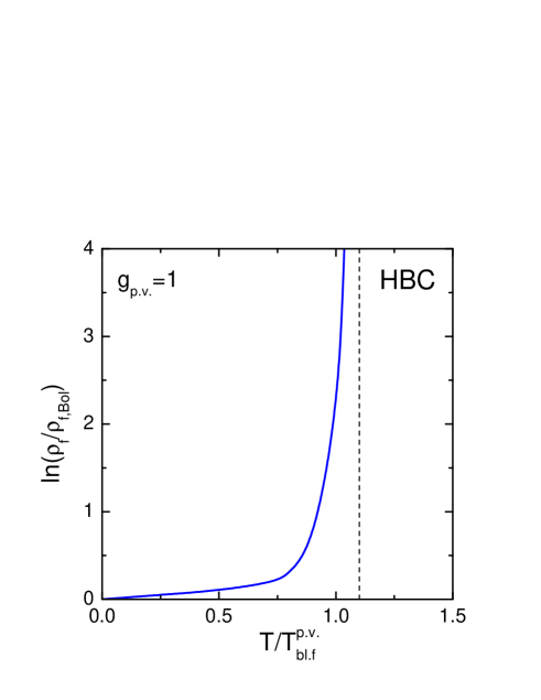
Figure 5: Logarithm of the ratio of the fermion density to the corresponding Boltzmann quantity for $g_{p.v}=1$ as function of the temperature in units of $T_{\rm bl.f}^{p.v}$. The vertical dash-line indicates the area of the HBC.

6.4 Correlation effects

The first diagram of $\Phi$, that we have studied, sums up all perturbative diagrams for the fermion Green function without crossing of the boson lines, cf. eq. (10). For the fermion-boson coupling under discussion, within the STL approximation, each diagram with the one crossed boson line (see eq. (11)) brings the suppression factor $\nu=\nu_{\tau}\nu_{\sigma}$ compared to the corresponding diagram with the same number of boson lines but without their crossing, cf. [5, 26]. Indeed, in the non-relativistic approximation for nucleons, $\nu_{\tau}=1/3$ is due to the non-commutation of the isospin $\tau$ matrices and in non-relativistic approximation for nucleons $\nu_{\sigma}=1/3$ is due to the non-commutation of the spin $\sigma$ matrices. Each product $\tau_{i}\tau_{i}\tau_{j}\tau_{j}$ yields factor 9, whereas each product $\tau_{i}\tau_{j}\tau_{i}\tau_{j}$ yields factor 3. The same statement is valid for $\sigma$ matrices. Concluding, we may retain only the first diagram (2) in $\Phi$ with an appropriate accuracy.

7 Towards the description of the state of hadron porridge

We discussed the behavior of model systems with a small fermion chemical potential, assuming for the sake of simplicity only one type of the interaction in each case, like the case of spin $\frac{1}{2}$ fermions (e.g., $N$) coupled with the scalar boson ($\sigma$), or with the vector boson ($\omega$ or $\rho$), or pseudo-scalar boson ($\pi$). This is, of course, a gross oversimplification. In reality nucleons couple with all mesons: $\sigma$, $\pi$, $\omega$, $\rho$, $K$, etc. Also high lying baryon resonances, like $\Delta$-isobar, $N^{*}(1440)$, hyperons, etc., interact with the nucleon and with each other. Moreover, mesons interact with each other. We may call such a system state the hadron porridge, bearing in mind that already at sufficiently low temperatures the quasiparticle approximation fails to describe baryons and that for $T\stackrel{{\scriptstyle\scriptstyle>}}{{\phantom{}{}_{\sim}}}m_{\pi}$ the continuum is blurred for all relevant hadrons, as we have shown it above on different concrete examples.

7.1 Hadron porridge in the low temperature limit

In the low temperature limit contributions of different mesons are summed up yielding resulting baryon resonance distribution and the total density of baryon resonances. The density of the spin $\frac{1}{2}$ baryon resonance of given species is easily recovered with the help of eq. (121):

$$\rho_{B^{*},(\pm)}=N_{B^{*}}\left(\frac{m_{B^{*}}T}{2\pi}\right)^{3/2}\mbox{exp}\left[-\frac{m_{B^{*}}\mp\mu_{B^{*}}}{T}\right]$$ (228)

$$+N_{B^{*}}\sum_{i}\left(\frac{m_{B^{*}_{i}}T}{2\pi}\right)^{3/2}\mbox{exp}\left[-\frac{m_{B^{*}_{i}}\mp\mu_{B^{*}_{i}}}{T}\right]\frac{1}{4\pi^{2}}$$

$$\times\left[g_{\sigma B^{*}B^{*}_{i}}^{2}I_{0s}\left(\frac{m_{B^{*}_{i}}}{m_{\sigma}}\right)+3g_{\pi B^{*}B^{*}_{i}}^{2}I^{0}_{0v}\left(\frac{m_{B^{*}_{i}}}{m_{\pi}}\right)\right.$$

$$\left.+g_{\omega B^{*}B^{*}_{i}}^{2}\left(I^{0}_{0v}\left(\frac{m_{B^{*}_{i}}}{m_{\omega}}\right)+\frac{3}{2}\frac{m_{\omega}}{m_{B^{*}_{i}}}I^{1}_{0v}\left(\frac{m_{B^{*}_{i}}}{m_{\omega}}\right)\right)\right.$$

$$\left.+3g_{\rho B^{*}B^{*}_{i}}^{2}\left(I^{0}_{0v}\left(\frac{m_{B^{*}_{i}}}{m_{\rho}}\right)+\frac{3}{2}\frac{m_{\rho}}{m_{B^{*}_{i}}}I^{1}_{0v}\left(\frac{m_{B^{*}_{i}}}{m_{\rho}}\right)\right)+...\right].$$

The summation is performed over all possible $s_{B^{*}}=1/2$ states including the given baryon state ($B^{*}$). Dots mean contributions of other meson exchanges and transitions between baryon states with different spins in initial and intermediate states in the diagram (8), e.g. ($N-K-\Lambda;\Lambda-K-N$), ($N-\pi-\Delta(\frac{3}{2},\frac{3}{2});\Delta(\frac{3}{2},\frac{3}{2})-\pi-N$), etc. Correlation effects are unimportant in the low temperature limit.

Numerically, already the contribution given by terms, which are explicitly presented in eq. (228), yields $R_{N}=\rho_{N}/\rho_{\rm Bol}^{N}\simeq 1.5$ for $T\sim m_{\pi}/2$ and for values of coupling constants, which we have used above; $\rho_{\rm Bol}^{N}$ is the nucleon density calculated with the help of the Boltzmann distribution. With taking into account of other contributions one may expect a further enhancement of the ratio.

We would like to pay attention to the enhancement of the population of baryon resonances, e.g., of the strange baryons, since contributions like ($\Delta-\pi-N;N-\pi-\Delta$), ($\Lambda-K-N;N-K-\Lambda$), etc, have no any additional exponential suppression compared to ($N-\pi-N;N-\pi-N$) terms, see eq. (122) and the corresponding discussion. Thus, the ratio of the densities of the given resonance and the nucleon, $R_{B^{*}/N}=\rho_{B^{*}}/\rho_{N}$, can be $\sim 1$ for the low lying baryon resonances, like $\Delta$, $\Lambda$, etc, for which $B^{*}$-meson-$N$ coupling constants are not suppressed.

7.2 Hadron porridge in the high temperature limit

Description of the hadron porridge in the high temperature limit, $T\stackrel{{\scriptstyle\scriptstyle>}}{{\phantom{}{}_{\sim}}}m_{\pi}$, is much more involved. Even in the STL approximation one gets coupled system of Dyson equations for different baryon resonance Green functions. Intensities of the multiple scattering entering the Dyson equation for the given resonance describe the coupling of this resonance to other resonances via the radiation and the absorption of different type of mesons. Correlation effects contribute to each vertex. The main correlation effect comes from scalar meson and vector meson terms. Moreover, boson effective masses and the $|\vec{q}|$ dependent terms of the boson spectrum are changed. In addition to all has been said the problem should be solved self-consistently.

Assume for a moment that correlation effects are suppressed. Then one deals with the sum of one-diagram $\Phi$-terms, see first diagram (2), where the boson line corresponds to any relevant meson and the fermion line relates to one of baryon resonances. Summation is over mesons and baryon resonances, including nucleons. Assume also that baryon resonance states decouple, i.e., coupling constants $g_{\mu B^{*}_{i},B^{*}_{j}}=0$, for $i\neq j$, $\mu$ is one of mesons. Then, above results obtained for the system with one type of baryons and one type of mesons are easily generalized to include all above mentioned types of the interaction. The contribution of the given baryon resonance $B^{*}$ in non-relativistic approximation for baryon resonances is obtained with the help of the replacement of the corresponding $J$ to the sum of relevant $J$’s, e.g.

$$J_{s}\rightarrow J_{\sigma,B^{*}}+J^{\omega,B^{*}}_{1}+J^{\rho,B^{*}}_{1}+J^{\pi,B^{*}}_{1}+...$$ (229)

Inclusion of cross-channel couplings ($g_{\mu B^{*}_{i},B^{*}_{j}}\neq 0$) and correlations make the problem much more involved. Correlations may yield a significant suppression of the resulting intensity of the multiple scattering compared to that given by (229). Moreover, going beyond the non-relativistic ansatz for baryons, that is necessary to do for $T\stackrel{{\scriptstyle\scriptstyle>}}{{\phantom{}{}_{\sim}}}T_{\rm bl.f}$, additionally complicates the consideration. We postpone a more detailed discussion of properties of the hadron porridge (including baryon resonances with a cross-channel coupling) to the subsequent paper.

8 Conclusion

The description of the hadron system with a small baryon chemical potential, $|\mu_{\rm bar}|\ll T$, at the finite temperature is essentially different from the description of the dense baryonic system $|\mu_{\rm bar}-m_{N}|\gg T$, cf. [14]. The former regime might be relevant for heavy ion collisions at RHIC and LHC, whereas the latter one, for SIS energies.

We treated the fermion-boson problem self-consistently considering first one heavy fermion and one lighter boson species. Then we estimated a role of correlation effects.

• We found that already at low temperatures, $T\ll T_{\rm bl.f}\sim m_{\pi}\simeq 140$ MeV, the nucleon 3-momentum distributions are enhanced compared to ordinary Boltzmann distributions. Quasiparticle approximation fails already in regime of a warm hadron liquid ($m_{b}^{2}/m_{f}\stackrel{{\scriptstyle\scriptstyle<}}{{\phantom{}{}_{\sim}}}T\ll\mbox{min}\{m_{b},T_{\rm bl.f}\}$), if this limit is indeed realized for the given particle species and if the coupling constant is $g\gg 1$.

• For a higher temperature (typical value is $T\sim T_{\rm bl.f}\sim m_{\pi}$) the hadron continuum is totally blurred. Effective masses of all hadrons are decreased and baryon widths are dramatically increased due to baryon rescatterings on bosons. Baryons play a role of a glue for mesons. The hadron liquid comes to the state of a hadron porridge.

• Scalar mesons, like $\sigma$, may undergo second order phase transition to the s-wave hot Bose condensate state for $T>T^{s}_{\rm cb}\sim T_{\rm bl.f}\simeq m_{\pi}$.

• Vector mesons, like $\omega$, $\rho$, may undergo first order phase transitions to s-wave hot Bose condensate states for $T>T^{v}_{\rm cb}\sim T_{\rm bl.f}\simeq m_{\pi}$. In the vicinity of the transition point the intensity of the multiple scattering is significantly increased leading to a critical opalescence.

• Pions may form a liquid hot Bose condensate for $T>T_{{\rm cb},1}^{p.v}\simeq m_{\pi}$ and with a subsequent increase of the temperature may undergo first order phase transition to the p-wave hot Bose condensate state. As in the vector case the intensity of the multiple scattering is significantly increased in the vicinity of the critical point.

• For $T>T_{\rm bl.f}$ fermions fill a rather dense packing state.

• The number of baryon resonances, like $\Lambda$, should be not much less than the number of nucleons. In particular cases, like for $\Delta$ isobar, one even may expect a higher abundance than for nucleons. The number of kaons, which interact with nucleons and hyperons, should be also large. One may expect the same effects for them, as for pions and $\sigma$’s, due to a strong s- and p-wave $KN\Lambda$ interactions.

When scalar meson mass reaches zero, the alternative state to the hot Bose condensate one could be the chiral phase state. To conclude, which state is preferable, one needs to study the chiral model, e.g., the linear sigma model, and one should include quark effects.

For the low temperature regime, as a guide, we used the Urbach rule. As a relevant approximation to simplify the self-consistent analysis of the hot fermion-boson system ($T\stackrel{{\scriptstyle\scriptstyle>}}{{\phantom{}{}_{\sim}}}m_{\pi}$), we exploited the soft thermal loop approximation. The latter approximation allowed us to solve the problem. The self-consistency of the approach is manifested in the fact that fermion Green functions completely loose their former pole shape. It is the consequence of multiple collisions of the fermion with bosons. On the other hand, bosons drop their masses interacting with modified fermions, that further stimulates the enhancement of the fermion width. Please notice that with only one $\Phi$ diagram we estimated $T_{\rm bl.f}\stackrel{{\scriptstyle\scriptstyle<}}{{\phantom{}{}_{\sim}}}m_{\pi}$. Attractive interactions of the nucleon with other meson species, being taken into account, could still decrease the value $T_{\rm bl.f}$. However we have shown that correlation effects in the scalar boson channel increase the value $T_{\rm bl.f}$. In the regime that we called “the hadron porridge” interactions between many resonance and meson species come into play. Scalar bosons contribute to vertices with participation of other mesons effectively suppressing vertices. We considered only some of interactions. Therefore it is hard to realistically estimate the actual value of $T_{\rm bl.f}$. Our rough estimates show that $T_{\rm bl.f}$ is somewhere in the vicinity of the pion mass ($140$ MeV). However further more detailed analysis is necessary.

We described the system in terms of only hadron degrees of freedom and we found a state of a hadron porridge for $T\stackrel{{\scriptstyle\scriptstyle>}}{{\phantom{}{}_{\sim}}}m_{\pi}$. In realistic situation quark-gluon degrees of freedom are also excited for $T\stackrel{{\scriptstyle\scriptstyle>}}{{\phantom{}{}_{\sim}}}m_{\pi}$. These effects may yield an additional diminishing of effective hadron masses due to the decrease of the quark condensate density with the increase of the temperature. The role of quark-gluon fluctuations rises with increase of the temperature. More likely, the system comes to a strongly correlated hadron-quark-gluon state or, in another words, a boiled hadron-quark-gluon porridge, (HQGP). Deconfinement, in a standard meaning, as the pure quark-gluon state, is probably delayed up to a higher temperature.

Our aim was to discuss qualitative effects. Thereby, we focused our study on simplified models. In order to quantify the consideration and to do an appropriate fit of experimental results, cf. [1, 2, 3], one needs to include $\Delta$ and other nucleon resonances and hyperons. In the meson sector one has to incorporate kaons. Meson-meson interaction, short-range correlations and other effects may also contribute essentially, as we have argued. Thermodynamical characteristics, like the pressure, energy, entropy still should be computed. Comparison with lattice results, cf. [12, 34], is then required. Moreover, one should supplement the consideration of in-medium properties of the system by a relevant model of the freeze out stage to match in-medium particle distributions to those distributions one observes at infinity. For sure the realistic consideration of strongly interacting heated nuclear system is a very complicated problem that needs a further study. We hope to return to these questions in forthcoming publications.

APPENDICES

Appendix A Formalism

A.1 Green functions and self-energies

In matrix $\{-,+\}$ notations there exist exact relations between two-point functions $F$ (Green functions and self-energies), cf. [4],

$$\widehat{F}^{R} = \widehat{F}^{--}-\widehat{F}^{-+}=\widehat{F}^{+-}-\widehat{F}^{++},\,\,\,$$

$$\widehat{F}^{A} = \widehat{F}^{--}-\widehat{F}^{+-}=\widehat{F}^{-+}-\widehat{F}^{++},$$ (230)

$\widehat{F}^{R}$ and $\widehat{F}^{A}$ are retarded and advanced two-point functions (operators in spin space). The co-contour functions are $\widehat{F}_{jk}=\sigma_{jl}\sigma_{km}\widehat{F}^{lm}$, $\sigma_{j}^{k}=\delta_{j}^{k}$, $\sigma_{jk}=\sigma^{jk}$, are standard $\sigma_{3}$ Pauli matrices, space indices $j,k,l,m=1,2,3$, $\delta_{j}^{k}=1$ for $j=k$ and $\delta_{j}^{k}=0$ for $j\neq k$.

The free fermion retarded Green function is

$$\widehat{G}_{f}^{0,R}(p)=\frac{\widehat{\Lambda}_{f}^{0}(p)}{p^{2}-m^{2}_{f}+i0}\equiv G_{f}^{0,R}(q)\widehat{\Lambda}_{f}^{0}(p),$$ (231)

and the free boson retarded Green function is

$$\widehat{G}_{b}^{0,R}(q)=\frac{\widehat{\Lambda}_{b}^{0}(q)}{q^{2}-m^{2}_{b}+i0}\equiv G_{b}^{0,R}(q)\widehat{\Lambda}_{b}^{0}(q),$$ (232)

$\widehat{\Lambda}_{f}^{0}$ and $\widehat{\Lambda}_{b}^{0}$ are corresponding spin structure operators of fermions and bosons, $p,q$ are 4-momenta. For the spin $1/2$ fermions one has $\widehat{\Lambda}_{f}^{0}=\hbox{$/$}\kern-4.91145pt\hbox{$q$}+m_{f}$ and for the scalar neutral boson one has $\widehat{\Lambda}_{b}^{0}=1$, $\hbox{$/$}\kern-4.91145pt\hbox{$q$}\equiv\gamma^{\mu}q_{\mu}$, $\gamma^{\mu}$ are Dirac matrices, $\mu=0,1,2,3$.

The spin structure of the free massive vector-boson propagator is given by

$$\widehat{\Lambda}_{b}^{0}=(g^{\mu\nu}-q^{\mu}q^{\nu}/m_{b}^{2}).$$ (233)

Using (1) it is convenient to introduce one-particle spectral and width functions (operators),

$$\widehat{A}_{i}=-2{\rm Im}\widehat{G}_{i}^{R}(q)=-2{\rm Im}\frac{1}{\widehat{M}_{i}+i\widehat{\Gamma}_{i}/2},\,\,\,\widehat{\Gamma}_{i}=-2{\rm Im}\widehat{\Sigma}_{i}^{R}\,.$$ (234)

The quantity

$$\widehat{M}_{i}=(\widehat{G}_{i}^{0,R})^{-1}-{\rm Re}\widehat{\Sigma}_{i}^{R}$$ (235)

demonstrates the deviation from the mass shell, $\widehat{M}=0$ on the mass shell in the matter, the relation that introduces quasiparticles.

At equilibrium all non-equilibrium Green functions, $\widehat{G}^{--}$, $\widehat{G}^{++}$, $\widehat{G}^{-+}$, and $\widehat{G}^{+-}$, are expressed through the retarded Green function, cf. [4], e.g.,

$$i\widehat{G}_{i}^{-+}=\mp n_{i}(q_{0})\widehat{A}_{i}(q),\,\,\,i\widehat{G}_{i}^{+-}=(1\mp n_{i}(q_{0}))\widehat{A}_{i}(q).$$ (236)

The upper sign corresponds to fermions, the lower, to bosons,

$$n_{i}(q_{0})=\frac{1}{\mbox{exp}[(q_{0}-\mu_{i})/T]\pm 1}$$ (237)

are fermion/boson occupations, $\mu_{i}$ are chemical potentials. Relations for $\widehat{\Sigma}_{i}^{-+}$ and $\widehat{\Sigma}_{i}^{+-}$ are similar to eqs (236):

$$i\widehat{\Sigma}_{i}^{-+} = -i\widehat{\Sigma}_{-+,i}=\mp n_{i}(q_{0})\widehat{\Gamma}_{i}(q),\,\,\,$$

$$i\widehat{\Sigma}_{i}^{+-} = -i\widehat{\Sigma}_{+-,i}=(1\mp n_{i}(q_{0}))\widehat{\Gamma}_{i}(q).$$ (238)

A.2 Particle-antiparticle separation

To deal with Green functions of physical particles and antiparticles we introduce the decomposition of Green functions into particle ($+$) and antiparticle ($-$) parts

$$\widehat{G}_{i}^{R}(q) = \Theta(q_{0})\widehat{G}_{i,(+)}^{R}(q)+\Theta(-q_{0})\widehat{G}_{i,(-)}^{A}(-q),$$

$$\widehat{G}_{i}^{-+}(q) = \Theta(q_{0})\widehat{G}_{i,(+)}^{-+}(q)+\Theta(-q_{0})\widehat{G}_{i,(-)}^{+-}(-q)\,,$$ (239)

$$\widehat{A}_{i}(q)=\Theta(q_{0})\widehat{A}_{i,(+)}(q)-\Theta(-q_{0})\widehat{A}_{i,(-)}(-q),$$ (240)

where $\Theta(x)=1$ for $x>0$ and $\Theta(x)=0$ for $x\leq 0$. These equations allow to reduce the integration in $q_{0}$ in self-energy diagrams to positive energies.

Spectral functions satisfy sum rules:

$$\frac{1}{N_{f}}\mbox{Tr}\int^{\infty}_{0}\gamma_{0}\left[\widehat{A}_{f,(+)}(q_{0},\vec{q})+\widehat{A}_{f,(-)}(q_{0},-\vec{q})\right]\frac{dq_{0}}{2\pi}=2,\,\,\,$$ (241)

$$\frac{1}{N_{b}}\mbox{Tr}\int^{\infty}_{0}q_{0}\left[\widehat{A}_{b,(+)}(q_{0},\vec{q})+\widehat{A}_{b,(-)}(q_{0},-\vec{q})\right]\frac{dq_{0}}{2\pi}=1.$$ (242)

The trace is taken over spin degrees of freedom. $N_{f}=(2s_{f}+1)$ is the fermion degeneracy factor and $N_{b}=(2s_{b}+1)$ is the boson degeneracy factor. For vector bosons sum rules are fulfilled separately for transversal ($N_{b}=3$, $\widehat{A}_{b,(\pm)}\rightarrow\widehat{A}_{b,(\pm)}^{t}$) and longitudinal ($N_{b}=1$, $\widehat{A}_{b,(\pm)}\rightarrow\widehat{A}_{b,(\pm)}^{l}$) degrees of freedom, see eqs (135), (136).

At the thermal equilibrium we may introduce occupations of physical particles and antiparticles as

$$n_{i,(+)}(q_{0})=n_{i}(q_{0})\Theta(q_{0}),\,\,\,n_{i,(-)}(q_{0})=-[n_{i}(-q_{0})\mp 1]\Theta(q_{0}),$$ (243)

$$n_{i,(+)}(q_{0}) = \frac{\Theta(q_{0})}{\mbox{exp}[(q_{0}-\mu_{i})/T]\pm 1},\,\,\,$$

$$n_{i,(-)}(q_{0}) = \frac{\Theta(q_{0})}{\mbox{exp}[(q_{0}+\mu_{i})/T]\pm 1}\,.$$ (244)

In-medium 3-momentum distributions of particles and antiparticles are obtained with the help of (A.2) from the definition of the zero component of the Noether 4-current, cf. [4],

$$\widehat{n}_{i,(+)}(\vec{q}) = \int^{\infty}_{0}\frac{\widehat{v}^{0}_{i}\widehat{A}_{i,(+)}(q)}{\mbox{exp}[(q_{0}-\mu_{i})/T]\pm 1}\frac{dq_{0}}{2\pi},$$

$$\widehat{n}_{i,(-)}(\vec{q}) = \int^{\infty}_{0}\frac{\widehat{v}^{0}_{i}\widehat{A}_{i,(-)}(q)}{\mbox{exp}[(q_{0}+\mu_{i})/T]\pm 1}\frac{dq_{0}}{2\pi},$$ (245)

$\widehat{v}^{0}_{i}=\gamma_{0}$ for fermions and $\widehat{v}^{0}_{i}=2q_{0}$ for bosons. The chemical potential of the antiparticle differs by the sign from the chemical potential of the particle. For the non-strange bosons the boson number is not conserved and the chemical potential $\mu_{b}=0$.

For a large size system we may neglect particle radiation from the surface and the baryon chemical potential is determined using the baryon number conservation

$$\rho_{\rm bar}=\rho_{f,(+)}-\rho_{f,(-)}.$$ (246)

The total Noether 4-current presented as the sum of partial contributions is conserved quantity [4]. It is expressed through the standard $A_{i}$ spectral functions. As it has been shown in [35], in thermal equilibrium the Noether current coincides with the conserved effective current (that can be derived from the Kadanoff–Baym kinetic equation), provided $\Phi$ derivable approximations are used. Refs [4] have demonstrated thermodynamical consistency of the approach. Thus the zero component of the Noether current coincides with the corresponding quantity obtained with the help of the standard thermodynamical relation, e.g. for the baryon density

$$\rho_{\rm bar}=\frac{\partial\Omega}{\partial\mu_{\rm bar}}.$$ (247)

Using the latter expression ref. [36] studied the nucleon – delta isobar – pion system in the virial limit of Dashen, Ma and Bernstein [37].

Particle and antiparticle Noether densities are

$$\rho_{i,(\pm)}=\mbox{Tr}\int\widehat{n}_{i,(\pm)}(\vec{q})\frac{d^{3}q}{(2\pi)^{3}}.$$ (248)

In the paper body we focus on the discussion of only slightly particle-antiparticle asymmetric systems and, as the limiting case, the particle-antiparticle symmetric system (heated hadron vacuum), bearing in mind possible applications to heavy ion collisions at RHIC and LHC energies, respectively. We assume $\rho_{\rm bar}\ll\rho_{f,(\pm)}$ and, thereby, $|\mu_{i}|/T\ll 1$. Then one may simplify above equations as

$$n_{i,(+)}(q_{0})=n_{i}^{sym}(q_{0})\left[1+\frac{\mu_{i}}{T}(1\mp n_{i}^{sym}(q_{0}))\right],$$ (249)

$$n_{i,(-)}(q_{0})=n_{i}^{sym}(q_{0})\left[1-\frac{\mu_{i}}{T}(1\mp n_{i}^{sym}(q_{0}))\right],$$ (250)

where the fermion/boson quantities are supplied by index “sym” for the particle-antiparticle symmetric system. For $\rho_{\rm bar}\stackrel{{\scriptstyle\scriptstyle>}}{{\phantom{}{}_{\sim}}}\rho_{f,(-)}$ particle-hole effects become important.

Appendix B Non-relativistic heavy fermions

In the paper body we have shown that in the low temperature limit heavy fermions can be treated as non-relativistic particles, since both the energy deviation from the bare fermion mass and the fermion momentum are much smaller than $m_{f}$. In the high temperature limit the non-relativistic approximation for fermions also holds in some temperature interval, namely, if conditions (72), (167) are fulfilled, the former for the case of the scalar or pseudo-scalar boson exchange, and the latter for the vector boson exchange. The relativistic study performed in the paper body justifies the validity of the non-relativistic approach for given cases. In order to come to non-relativistic expressions from relativistic ones we need to expand $G_{1}\simeq G_{2}$ near the fermion mass-shell, $p^{2}=m_{f}^{2}$, and to introduce the fermion non-relativistic self-energy (40) averaged over spin degrees of freedom.

Suppose, conditions for the non-relativistic approximation for fermions are fulfilled. Then the consideration is simplified. The free fermion particle/antiparticle Green function obeys the equation

$$[G_{f}^{0,R}(p_{0},\vec{p})]^{\rm n.rel}=\frac{1}{p_{0}-\vec{p}^{\,2}/(2m_{f})+i0},$$ (251)

instead of eq. (231) in relativistic case. The spectral function (instead of (234), (235)) is given by

$$A_{f}^{\rm n.rel}=\frac{\Gamma_{f}^{\rm n.rel}}{[M_{f}^{\rm n.rel}]^{2}+[\Gamma_{f}^{\rm n.rel}]^{2}/4},$$ (252)

with $M_{f}^{\rm n.rel}=p_{0}-\vec{p}^{\,2}/(2m_{f})-[{\rm Re}\Sigma^{R}_{f}]^{\rm n.rel}$. The sum rule is changed accordingly. Fermion particle and antiparticle distributions and densities are

$$n_{f}^{\rm n.rel}(\vec{q}) = \int^{\infty}_{-\infty}\frac{A_{f}^{\rm n.rel}(q)}{\mbox{exp}[(q_{0}\mp\mu_{f})/T]+1}\frac{dq_{0}}{2\pi},$$ (253)

$$\rho_{f}^{\rm n.rel}=2\int n_{f}^{\rm n.rel}(\vec{q})\frac{d^{3}q}{(2\pi)^{3}},$$ (254)

cf. eqs (A.2) and (248). Further to shorten notations we suppress index ${}^{\prime\prime}{\rm non-rel}^{\prime\prime}$.

Thermodynamic quantities are easily found. The Noether energy–momentum tensor [4]

$$\Theta^{\mu\nu}/V = \mbox{Tr}\left(\frac{1}{2}\right)_{\rm{n.b.}}\sum_{i}\int(\mp)iG^{-+}_{i}v^{\mu}_{i}p^{\nu}_{i}\frac{d^{4}p}{(2\pi)^{4}}$$ (255)

$$+ g^{\mu\nu}\left({\mathcal{E}}^{\rm{int}}-{\mathcal{E}}^{\rm{pot}}\right)+{\mathcal{E}}_{\rm{(der.)}}^{\mu\nu}$$

is exactly conserved within the $\Phi$ derivable scheme. Here $V$ is the system volume, $i=\{f,b\}$ indicates that sum is over all non-relativistic fermions and relativistic bosons. Extra factor $\left(\frac{1}{2}\right)_{\rm{n.b.}}$ occurs only for neutral bosons. The velocity $v_{i}^{\mu}=\partial G^{0,R}_{i}/\partial p_{\mu}$. The potential energy ${\mathcal{E}}^{\rm{pot}}$, which a probe particle with Wigner density $G^{-+}$ would have due to the interaction with all other particles in the system, is

$${\mathcal{E}}^{\rm{pot}}=\mbox{Tr}\left(\frac{1}{2}\right)_{\rm{n.b.}}\sum_{i}\int\frac{d^{4}p_{i}}{(2\pi)^{4}}\left[(\mp)iG^{-+}_{i}{\rm Re}\Sigma^{R}_{i}+(\mp)i\Sigma^{-+}_{i}{\rm Re}G^{R}_{i}\right],$$ (256)

and the interaction energy ${\mathcal{E}}^{\rm{int}}$ is simply related to ${\mathcal{E}}^{\rm{pot}}$,

$${\mathcal{E}}^{\rm{int}}=\frac{2}{\alpha}{\mathcal{E}}^{\rm{pot}},$$ (257)

in case all the interaction vertices of the theory have the same number of lines attached to them. For the two-fermion–one-boson interaction, see (2), one has $\alpha=3$, that results in ${\mathcal{E}}^{\rm{int}}=\frac{2}{3}{\mathcal{E}}^{\rm{pot}}$. The additional term ${\mathcal{E}}_{\rm{(der.)}}^{\mu\nu}$ appears in eq. (255) only in the case of derivative coupling, cf. [35]. The energy and the pressure at the quasi-equilibrium are given by

$$E=\Theta^{00},\,\,\,\,P=-\Omega/V=\frac{1}{3}\left(\Theta^{11}+\Theta^{22}+\Theta^{33}\right),$$ (258)

$$\Omega=V\mbox{Tr}\sum_{i}\int\frac{d^{4}p_{i}}{(2\pi)^{4}}n_{i}(p_{0i})\left\{-2\mbox{Im}\,\,\mbox{ln}\left[-G_{i}^{R}(p_{0i}+i0,\vec{p}_{i})\right]\right.$$

$$\left.-\mbox{Re}G_{i}^{R}\Gamma_{i}-A_{i}\mbox{Re}\Sigma_{i}^{R}\right\}+\Phi_{T},\quad\Phi_{T}=-iT\Phi,$$ (259)

$\Phi$ is the functional expressed in terms of non-equilibrium contour Green functions, cf. [4]. The expression for the entropy is as follows

$$s^{0} = S/V=-\mbox{Tr}\sum_{i}\int\frac{d^{4}p_{i}}{(2\pi)^{4}}\frac{\partial n_{i}(p_{0i})}{\partial T}$$ (260)

$$\times \left[-2\mbox{Im}\;\ln\left[-G_{i}^{R}(p_{0i}+i0,\vec{p}_{i})\right]-\mbox{Re}G_{i}^{R}\Gamma_{i}-A_{i}\mbox{Re}\Sigma_{i}^{R}\right]-\frac{\partial\Phi_{T}}{\partial T}.$$

This way one may recover all necessary thermodynamic characteristics of the system.

References

- [1] T. Chujo et al, nucl-ex/0209027; ; D. Querdane et al, nucl-ex/0212001; C. Ronald et al., nucl-ex/0212006; T. S. Ullrich, nucl-ex/0305018.
- [2] J. Rafelski, and J. Letessier, Acta Phys. Polon. B34 (2003) 5791.
- [3] P. Braun-Munzinger, D. Magestro, K. Redlich, and J. Stachel, Phys.Lett. B518 (2001) 41; P. Braun-Munzinger, K. Redlich, and J. Stachel, Particle production in heavy ion collisions, Quark Gluon Plasma 3, eds. R.C. Hwa and Xin-Nian Wang, World Sci. Pub. (2003), nucl-th/0304013; P. Braun-Munzinger, J. Stachel, Ch. Wetterich, nucl-th/0311005.
- [4] Yu.B. Ivanov, J. Knoll, and D.N. Voskresensky, Nucl. Phys. A657 (1999) 413; ibid A672 (2000) 313.
- [5] A. M. Dyugaev, JETP Lett. 58 (1993) 886.
- [6] B.I. Shklovskii and A.L. Efros, Electronic properties of Doped Semiconductors, Springer-Verlag, N.Y., 1984; D. Dunn, Phys. Rev. 174 (1968) 855.
- [7] D. B. Blaschke, and K. A. Bugaev, nucl-th/0311021.
- [8] M. Gazdzicki, and M.I. Gorenstein, Acta Phys. Polon. B30 (1999) 2705.
- [9] N.O. Agasian, and S.M. Fedorov, JETP Lett. 78 (2003) 607.
- [10] R. Rapp, nucl-th/0209081.
- [11] D.N. Voskresensky, nucl-th/0306077, nucl-th/0312016, Phys. Rev. C69 (2004) 065209.
- [12] Z. Fodor, and S.D. Katz, JHEP 0203 (2002) 014; F. Csikor, G.I. Egri, Z. Fodor, S.D. Katz, K.K. Szabo, and A.I. Tothet, hep-lat/0301027; F. Karsch, and E. Laermann, hep-lat/0305025.
- [13] D.N. Voskresensky, and A.V. Senatorov, Sov. Phys. Dokl. 33 (1988) 845; A.V. Senatorov, and D.N. Voskresensky, Phys. Lett. B219 (1989) 31.
- [14] A. B. Migdal, E. E. Saperstein, M. A. Troitsky, and D.N. Voskresensky, Phys. Rep. 192 (1990) 179.
- [15] G. Baym, Phys. Rev. 127 (1962) 1391.
- [16] E.M. Lifshitz, and L.P. Pitaevskii, Physical Kinetics, Pergamon, 1981.
- [17] J.-P. Blaizot, and E. Iancu, Phys.Rep. 359 (2002) 355.
- [18] H. van Hees, and J. Knoll, Phys. Rev. D65 (2002) 025010, 105005; D66 (2002) 025028.
- [19] M. Schmidt, G. Röpke, and H. Schulz, Annals Phys. 202 (1990) 57.
- [20] Yu. B. Ivanov, J. Knoll, H. van Hees, and D. N. Voskresensky, Phys. At. Nucl. 64 (2001) 652.
- [21] J. Knoll, and D. N. Voskresensky, Phys. Lett. B351 (1995) 43; Annals Phys. 249 (1996) 532.
- [22] R. Rapp, and J. Wambach, Adv. Nucl. Phys. 25 (2000) 1; J. Wambach, Prog. Part. Nucl. Phys. 50 (2003) 615.
- [23] D.N. Voskresensky, JETP 78 (1994) 793; Sov. J. Nucl. Phys. 59 (1996) 2015.
- [24] K. Wehrberger, C. Bedu, and F. Beck, Nucl. Phys. A504 (1989) 797.
- [25] B.J. Dias, A. Valcarce, and F. Fernandez, nucl-th/0308086.
- [26] A.M. Dyugaev, Sov. J. Nucl. Phys. 38 (1983) 680.
- [27] E. E. Kolomeitsev, and D. N. Voskresensky, Phys. Rev. C68 (2003) 015803.
- [28] D.N. Voskresensky, and I.N. Mishustin, Sov. J. Nucl. Phys. 35 (1982) 667.
- [29] R. Rapp, and J. Wambach, Nucl. Phys. A573 (1994) 626.
- [30] N. K. Glendenning, Phys. Rep. 342 (2001) 393.
- [31] H. Shiomi, and T. Hatsuda, Phys. Lett. B334 (1994) 281.
- [32] J.I. Kapusta, Finite-temperature Field Theory, Cambrigde Univ. Press, 1989.
- [33] D.N. Voskresensky, Nucl. Phys. A555 (1993) 293.
- [34] F. Karsch, K. Redlich, and A. Tawfik, Eur. Phys. J. C29 (2003) 549; Phys. Lett. B571 (2003) 67.
- [35] Yu.B. Ivanov, J. Knoll, and D.N. Voskresensky, Phys. At. Nucl. 66 (2003) 1902; nucl-th/0303006.
- [36] W. Weinhold, B. Friman, and W. Nörenberg, Phys. Lett. B433 (1998) 236.
- [37] R. Dashen, S.-K. Ma, and H.J. Bernstein, Phys. Rev. 187 (1969) 345.