A RELIEF TO THE SUPERSYMMETRIC FINE TUNING PROBLEM

Abstract

As is well known, electroweak breaking in the MSSM requires substantial fine-tuning. We explain why this fine tuning problem is abnormally acute, and this allows to envisage possible solutions to this undesirable situation. Following these ideas, we review some recent work which shows how in models with SUSY broken at a low scale (not far from the TeV) this fine-tuning can be dramatically reduced or even absent.

IFT-UAM/CSIC-04-03

1 The abnormally acute fine tuning problem of the MSSM

According to general arguments, based on the size of the quadratically-divergent radiative corrections to the Higgs mass parameter in the Standard Model (SM), the request of no fine-tuning in the electroweak breaking implies that the scale of new physics should be $\Lambda\stackrel{{\scriptstyle<}}{{{}_{\sim}}}$ few TeV . However, in the minimal supersymmetric Standard Model (MSSM), the absence of fine tuning requires that the masses of the new supersymmetric particles should be $\stackrel{{\scriptstyle<}}{{{}_{\sim}}}$ few hundred GeV. Actually, the available experimental data already imply that the ordinary MSSM is fine tuned at least by one part in 10. Clearly, the fine tuning of the MSSM is abnormally acute. Let us review the reasons for this (undesirable) situation[1]. (For related work see refs. [2, 3, 4, 5, 6, 7])

In the MSSM the Higgs sector consists of two $SU(2)_{L}$ doublets, $H_{1}$, $H_{2}$. The (tree-level) scalar potential for the neutral components, $H^{0}_{1,2}$, of these doublets reads

$$V^{\rm MSSM}=m_{1}^{2}|H_{1}^{0}|^{2}+m_{2}^{2}|H_{2}^{0}|^{2}-(m_{3}^{2}H_{1}^{0}H^{0}_{2}+{\rm h.c.})+\frac{1}{8}(g^{2}+g_{Y}^{2})(|H^{0}_{1}|^{2}-|H^{0}_{2}|^{2})^{2},$$ (1)

with $m_{1,2}^{2}=\mu^{2}+m_{H_{1,2}}^{2}$ and $m_{3}^{2}=B\mu$, where $m_{H_{i}}^{2}$ and $B$ are soft masses and $\mu$ is the Higgs mass term in the superpotential, $W\supset\mu H_{1}\cdot H_{2}$. Minimization of $V^{\rm MSSM}$ leads to a vacuum expectation value (VEV) $v^{2}\equiv 2(\langle H^{0}_{1}\rangle^{2}+\langle H^{0}_{2}\rangle^{2})$ and thus to a mass for the $Z^{0}$ gauge boson, $M_{Z}^{2}=\frac{1}{4}(g^{2}+g_{Y}^{2})v^{2}$.

The parameters of eq.(1), in particular $m_{i}^{2}$, depend on the initial parameters, $p_{\alpha}$, which for the MSSM are the soft masses, the $\mu-$parameter, etc. at the initial (high energy) scale. Therefore, $v^{2}=v^{2}(p_{1},p_{2},\cdots)$. The fine tuning associated to $p_{\alpha}$ is usually defined by $\Delta_{p_{\alpha}}$ as [2]

$${\delta v^{2}\over v^{2}}=\Delta_{p_{\alpha}}{\delta p_{\alpha}\over p_{\alpha}}\ ,$$ (2)

where $\delta v^{2}$ is the change induced in $v^{2}$ by a change $\delta p_{\alpha}$ in $p_{\alpha}$. Absence of fine tuning requires that $\Delta_{p_{\alpha}}$ should not be larger than ${\cal O}(10)$.

Along the breaking direction in the $H_{1}^{0},H_{2}^{0}$ space, the potential (1) can be written in a SM-like form:

$$V={1\over 2}m^{2}v^{2}+{1\over 4}\lambda v^{4}\ ,$$ (3)

where $\lambda$ and $m^{2}$ are functions of the $p_{\alpha}$ parameters and $\tan\beta$ ($\equiv\langle H^{0}_{2}\rangle/\langle H^{0}_{1}\rangle$), in particular

$$m^{2}=c_{\beta}^{2}\,m_{1}^{2}(p_{\alpha})+s_{\beta}^{2}\,m_{2}^{2}(p_{\alpha})-s_{2\beta}\,m_{3}^{2}(p_{\alpha})\ .$$ (4)

Minimization of (3) leads to

$$v^{2}={-m^{2}\over\lambda}\ .$$ (5)

In the SM, $m^{2}$ is an input parameter that receives important radiative corrections, in particular the quadratically-divergent ones mentioned above: $\delta m^{2}\propto{\Lambda^{2}\over 16\pi^{2}v^{2}}(m_{t}^{2}+\cdots)$. Hence, a tuning between the tree-level and the one-loop contributions is required to keep $m^{2}$ of electroweak size, and this sets the naturalness bound on $\Lambda$.

In the MSSM this type of corrections are absent. However, $m^{2}$ receives important logaritmic corrections $\delta m^{2}\propto{\tilde{m}^{2}\over 16\pi^{2}}\log{M_{X}^{2}\over\tilde{m}^{2}}$, where $\tilde{m}$ is a typical soft mass and $M_{X}$ represents the higher scale at which the soft breaking terms are generated. These corrections can be viewed as the effect of the RG running of $m^{2}$ from $M_{X}$ down to the electroweak scale. Typically, the large logarithms and the numerical factors compensate the one-loop factor, so that the corrections are quite large, ${\cal O}(\tilde{m}^{2})$ [actually the tree-level values of $m_{i}^{2}$, and thus of $m^{2}$, partly have a SUSY-breaking origin and are expected to be ${\cal O}(\tilde{m}^{2})$ as well]. This is a first reason why the naturalness bounds on the supersymmetric masses are more stringent than suggested by the SM argument based on the SM quadratically-divergent corrections . To be concrete, for large $\tan\beta$ and $M_{X}=M_{GUT}$,

$$m^{2}=m_{1}^{2}c^{2}_{\beta}+m_{2}^{2}s^{2}_{\beta}-m_{3}^{2}s_{2\beta}\simeq 1.01\mu^{2}-2.31\tilde{m}^{2}\ ,$$ (6)

where, for simplicity, we have taken $\tilde{m}$ as the universal value of gaugino and scalar soft masses and trilinear soft terms, $M=m=A=\tilde{m}$. The presence of a sizeable RG coefficient in front of $\tilde{m}^{2}$ shows that the one-loop factor has been largely compensated.

A second (and even more important) reason for the unusual fine tuning of the MSSM is the following. From eq.(5), we note that $\Delta\sim{\tt m_{i}^{2}}/(\lambda v^{2})$, where ${\tt m_{i}^{2}}$ are the (potentially large) individual contributions to $m^{2}$ [see eq.(6)]. Now, for the MSSM $\lambda$ turns out to be quite small:

$$\lambda_{\rm MSSM}={1\over 8}(g^{2}+g_{Y}^{2})\cos^{2}2\beta\ \simeq\ {1\over 15}\cos^{2}2\beta\ ,$$ (7)

which implies a fine tuning $\stackrel{{\scriptstyle>}}{{{}_{\sim}}}15$ times larger than expected from naive dimensional considerations.

The previous $\lambda_{\rm MSSM}$ was evaluated at tree-level but radiative corrections make $\lambda$ larger, thus reducing the fine tuning[3, 4]. Since $m_{h}^{2}\sim 2\lambda v^{2}$, the ratio $\lambda_{\rm tree}/\lambda_{\rm 1-loop}$ is basically the ratio $(m_{h}^{2})_{\rm tree}/(m_{h}^{2})_{\rm 1-loop}$, so for large $\tan\beta$ the previous factor 15 is reduced by a factor $M_{Z}^{2}/m_{h}^{2}$. It is important to notice that, although for a given size of the soft terms the radiative corrections reduce the fine tuning, the requirement of sizeable radiative corrections implies itself large soft terms, which in turn worsens the fine tuning. More precisely, for the MSSM $\delta_{\rm rad}\lambda\propto\log(M_{\rm SUSY}^{2}/m_{t}^{2})$, where $M_{\rm SUSY}$ is an average of stop masses [in the universal case, $M_{\rm SUSY}^{2}\simeq 3.6\tilde{m}^{2}+m_{t}^{2}+({\rm D-terms})$]. Hence, $\lambda$ can only be radiatively enhanced by increasing $M_{\rm SUSY}^{2}$, and thus $\tilde{m}$ and the individual ${\tt m_{i}^{2}}$. A given increase in $M_{\rm SUSY}^{2}$ reflects linearly in ${\tilde{m}}^{2}$ and only logarithmically in $\lambda$, so the fine tuning $\Delta\sim{\tt m_{i}^{2}}/(\lambda v^{2})$ gets usually worse.

On the other hand, for the MSSM sizeable radiative corrections to the Higgs mass (and thus to $\lambda$) are in fact mandatory. This can be easily understood by writing the tree-level and the dominant 1-loop correction to the theoretical upper bound on $m_{h}$ in the MSSM:

$$m_{h}^{2}\leq M_{Z}^{2}\cos^{2}2\beta+{3m_{t}^{4}\over 2\pi^{2}v^{2}}\log{M_{\rm SUSY}^{2}\over m_{t}^{2}}+...$$ (8)

where $m_{t}$ is the (running) top mass ($\simeq 167$ GeV for $M_{t}=174$ GeV). Since the experimental lower bound, $(m_{h})_{\rm exp}\geq 115$ GeV, exceeds the tree-level contribution, the radiative corrections must be responsible for the difference, and this translates into a lower bound on $M_{\rm SUSY}$:

$$M_{\rm SUSY}\;\stackrel{{\scriptstyle>}}{{{}_{\sim}}}\;e^{-2.1\cos^{2}2\beta}e^{\left({m_{h}}/{62\ {\rm GeV}}\right)^{2}}m_{t}\;\stackrel{{\scriptstyle>}}{{{}_{\sim}}}\;3.8\ m_{t}\ ,$$ (9)

where the last figure corresponds to $m_{h}=115$ GeV and large $\tan\beta$, i.e. the most favorable case for the fine tuning. The last equation implies sizeable soft terms, $\tilde{m}\stackrel{{\scriptstyle>}}{{{}_{\sim}}}2m_{t}$, which in turn translates into large fine-tunings, $\Delta\stackrel{{\scriptstyle>}}{{{}_{\sim}}}{\cal O}(10)$.

The discussion of this section about the size of the fine-tuning in the MSSM is reflected in the plot of fig.1

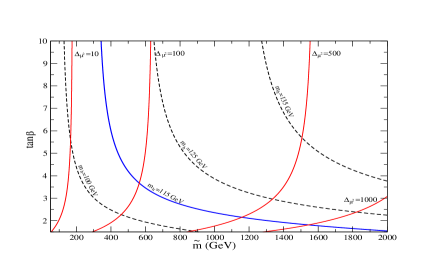
Figure 1: Fine tuning in the MSSM (measured by $\Delta_{\mu^{2}}$, solid lines) in the $(\tilde{m},\tan\beta)$ plane. Dashed lines are contour lines of constant Higgs mass.

2 Possible solutions

As discussed above, the fine tuning of the MSSM is much more severe than naively expected due, basically, to the smallness of the tree-level Higgs quartic coupling, $\lambda_{\rm tree}$ and, also, to the large magnitude of the RG effects. The problem is worsened by the fact that sizeable radiative corrections (and thus sizeable soft terms) are needed to satisfy the experimental bound on $m_{h}$. This is also due to the smallness of $\lambda_{\rm tree}$: if it were bigger, radiative corrections would not be necessary. In consequence, the most efficient way of reducing the fine tuning is to consider supersymmetric models where $\lambda_{\rm tree}$ is larger than in the MSSM. Then let us focus on $\Delta_{\mu^{2}}$, which can be writen as [1]

$$\Delta_{\mu^{2}}\simeq\frac{\mu^{2}}{m^{2}}\frac{\partial m^{2}}{\partial\mu^{2}}\simeq-\frac{\mu^{2}}{\lambda v^{2}}\simeq-2\frac{\mu^{2}}{m_{h}^{2}}\ .$$ (10)

Strictly speaking, $m_{h}^{2}$ in (10) is the Higgs mass matrix element along the breaking direction, but in many cases of interest it is very close to one of the mass eigenvalues. Therefore

$$\Delta_{\mu^{2}}\simeq\Delta_{\mu^{2}}^{\rm MSSM}\left[\frac{m_{h}^{\rm MSSM}}{m_{h}}\right]^{2}\left[\frac{\mu}{\mu^{\rm MSSM}}\right]^{2}\ .$$ (11)

This equation shows the two main ways in which a theory can improve the MSSM fine tuning: increasing $m_{h}$ and/or decreasing $\mu$. The first way corresponds to increasing $\lambda$. The second, for a given $m_{h}$, corresponds to reducing the size of the soft terms [from (6) EW breaking requires the size of $\mu^{2}$ to be proportional to the overall size of the soft squared-masses], which is only allowed if radiative contributions are not essential to raise $m_{h}$. Both improvements indeed concur for larger $\lambda_{\rm tree}$.

The possibility of having tree-level quartic Higgs couplings larger than in the MSSM is natural in scenarios in which the breaking of SUSY occurs at a low-scale (not far from the TeV scale) [8, 9, 10, 11]. Besides, in that framework the RG effects are largely suppressed due to the low SUSY breaking scale. As noticed above, this is also welcome for the fine tuning issue. These ideas are developed in detail in the next sections.

3 Low-scale SUSY breaking

In any realistic breaking of SUSY (SUSY), there are two scales involved: the SUSYscale, say $\sqrt{F}$, which corresponds to the VEVs of the relevant auxiliary fields in the SUSYsector; and the messenger scale, $M$, associated to the interactions that transmit the breaking to the observable sector. These operators give rise to soft terms (such as scalar soft masses), but also hard terms (such as quartic scalar couplings):

$$m_{\rm soft}^{2}\sim{F^{2}\over M^{2}}\ ,\;\;\;\;\lambda_{\makebox[24.18501pt][l]{$\line(4,1){19.0}$ {\tiny{SUSY}}}}\sim{F^{2}\over M^{4}}\sim{m_{\rm soft}^{2}\over M^{2}}\ .$$ (12)

Phenomenology requires $m_{\rm soft}={\cal O}(1\,{\rm TeV})$, but this does not fix the scales $\sqrt{F}$ and $M$ separately. So, (unlike in the MSSM) the scales $\sqrt{F}$ and $M$ could well be of similar order (thus not far from the TeV scale). This happens in the so-called low-scale SUSYscenarios[8, 9, 10, 11]. In this framework, the hard terms of eq. (12), are not negligible anymore and hence the SUSYcontributions to the Higgs quartic couplings can be easily larger than the ordinary MSSM value (7). As discussed in the previous section, this is exactly the optimal situation to ameliorate the fine tuning problem.

As a simple example, suppose that the Kähler potential contains the operator $K\ \supset\ -\frac{1}{M^{2}}|T|^{2}|H|^{2}+\cdots$, where $H$ denotes any Higgs superfield and $T$ is the superfield responsible for SUSY, $\langle F_{T}\rangle\neq 0$. Then, the above nonrenormalizable interaction produces soft terms as well as hard terms, which is schematically represented in the diagrams of Fig. 2. Notice that $m_{\rm soft}^{2}\sim|F_{T}|^{2}/M^{2}$, $\lambda_{\makebox[24.18501pt][l]{$\line(4,1){19.0}$ {\tiny{SUSY}}}}\sim|F_{T}|^{2}/M^{4}\sim m_{\rm soft}^{2}/M^{2}$, in agreement with (12). More generally, the Higgs potential has the structure of a generic two Higgs doublet model (2HDM), with $T$-dependent coefficients. (If the $T$ field is heavy enough, it can be integrated out and one ends up with a truly 2HDM.)

Figure 2: Higgs soft masses and hard quartic couplings that arise from the Kähler operator discussed in sect.3.

The appearance of non-conventional quartic couplings has a deep impact on the pattern of EW breaking [11]. In the MSSM, the existence of D-flat directions, $|H_{1}|=|H_{2}|$, imposes the well-known condition, $m_{1}^{2}+m_{2}^{2}-2|m_{3}^{2}|>0$, in order to avoid a potential unbounded from below along such directions. However, the boundedness of the potential can now be simply ensured by the contribution of the extra quartic couplings, and this opens up many new possibilities for EW breaking. For example, the universal case $m_{1}^{2}=m_{2}^{2}$ is now allowed, as well as the possibility of having both $m_{1}^{2}$ and $m_{2}^{2}$ negative (with $m_{3}^{2}$ playing a minor role). In addition, and unlike in the MSSM, there is no need of radiative corrections to destabilize the origin, and EW breaking generically occurs already at tree-level (which is just fine since the effects of the RG running are small as the cut-off scale is $M$). Moreover, this tree-level breaking (which is welcome for the fine tuning issue, as discussed in sect. 2) occurs naturally only in the Higgs sector [11], as desired.

Finally, the fact that quartic couplings are very different from those of the MSSM changes dramatically the Higgs spectrum and properties. In particular, the MSSM upper bound on the mass of the lightest Higgs field no longer applies, which has also an important and positive impact on the fine tuning problem, as is clear from the discussion after eq. (11).

4 A concrete model

In this section we evaluate numerically the fine tuning involved in the EW symmetry breaking in a particular model with low-scale SUSYand compare it with that of the MSSM. We choose a model first introduced (as ”example A”) in [11] and analyzed there for its own sake. We show now that the fine tuning problem is greatly softened in this model even if it was not constructed with that goal in mind.

The superpotential is given by

$$W=\Lambda_{S}^{2}T+\mu H_{1}\cdot H_{2}+{\ell\over 2M}(H_{1}\cdot H_{2})^{2}\ ,$$ (13)

and the Kähler potential is

$$K = |T|^{2}+|H_{1}|^{2}+|H_{2}|^{2}$$ (14)

$$- {\alpha_{t}\over 4M^{2}}|T|^{4}+{\alpha_{1}\over M^{2}}|T|^{2}\left(|H_{1}|^{2}+|H_{2}|^{2}\right)+{e_{1}\over 2M^{2}}\left(|H_{1}|^{4}+|H_{2}|^{4}\right)\ .$$

(All parameters are real with $\alpha_{t}>0$.) Here $T$ is the singlet field responsible for the breaking of supersymmetry, $\Lambda_{S}$ is the SUSYscale and $M$ the ‘messenger’ scale (see previous section). The typical soft masses are $\sim\tilde{m}\equiv\Lambda_{S}^{2}/M$. In particular, the mass of the scalar component of $T$ is ${\cal{O}}(\tilde{m})$ and, after integrating this field out, the effective potential for $H_{1}$ and $H_{2}$ is a 2HDM with very particular Higgs mass terms:

$$m_{1}^{2}=m_{2}^{2}=\mu^{2}-\alpha_{1}\tilde{m}^{2}\ ,\;\;\;\;m_{3}^{2}=0\ ,$$ (15)

and Higgs quartic couplings like those of the MSSM plus contributions of order $\mu/M$ and $\tilde{m}^{2}/M^{2}$:

$$\lambda_{1}=\lambda_{2} = {1\over 4}(g^{2}+g_{Y}^{2})+2\alpha_{1}^{2}{\tilde{m}^{2}\over M^{2}}\ ,$$

$$\lambda_{3} = {1\over 4}(g^{2}-g_{Y}^{2})+{2\over M^{2}}(\alpha_{1}^{2}\tilde{m}^{2}-e_{1}\mu^{2})\ ,$$

$$\lambda_{4} = -{1\over 2}g^{2}-2\left(e_{1}+2{\alpha_{1}^{2}\over\alpha_{t}}\right){\mu^{2}\over M^{2}}\ ,$$

$$\lambda_{5} = 0\ ,$$

$$\lambda_{6}=\lambda_{7} = {\ell\mu\over M}\ .$$ (16)

The minimization condition for $v$ is given by eq.(5) with

$$\lambda=\sum_{i=1}^{7}d_{i}(\beta)\lambda_{i}(p_{\alpha}),\;\;\;\;\;\;\vec{d}=({1\over 2}c^{4}_{\beta},{1\over 2}s^{4}_{\beta},s^{2}_{\beta}c^{2}_{\beta},s^{2}_{\beta}c^{2}_{\beta},s^{2}_{\beta}c^{2}_{\beta},c^{2}_{\beta}{s_{2\beta}},s^{2}_{\beta}{s_{2\beta}})\ ,$$ (17)

and there is an additional (solvable) minimization equation for $\tan\beta$ [1]. The explicit expressions for $v$, $\sin 2\beta$ and the spectrum of Higgs masses can be found in [11, 1]. The corresponding expression for $\Delta_{\mu^{2}}$, as evaluated from eq.(2), is

$$\Delta_{\mu^{2}}=-{\mu^{2}\over\lambda v^{2}}\left[1+v^{2}\left({ls_{2\beta}\over 2\mu M}-{1\over M^{2}}(e_{1}+{\alpha_{1}^{2}\over\alpha_{t}})s_{2\beta}^{2}\right)\right]\ .$$ (18)

To make clear the difference of behaviour with respect to the MSSM, we plot in Fig. 3 $\Delta_{\mu^{2}}$ vs. $m_{h}$, taking $\mu=330$ GeV, $\tilde{m}=550$ GeV, $e_{1}=-2$, $\alpha_{t}=1$, $l$ chosen to give $\tan\beta=10$, and varying $\tilde{m}/M$ from 0.05 to 0.8. In this way we can study the effect on the fine tuning of varying $\lambda$ when the low energy mass scales ($\mu$ and $\tilde{m}$) are kept fixed. When $\tilde{m}/M$ is small (and this implies that $\mu/M$ is also small), the unconventional corrections to quartic couplings are not very important and the Higgs mass tends to its MSSM value. As $\tilde{m}/M$ increases, the tree level Higgs mass (or $\lambda$) also grows and this makes $\Delta_{\mu^{2}}$ decrease with $m_{h}$, just the opposite of the MSSM behaviour.

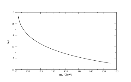
Figure 3: Fine tuning in a low-scale SUSY breaking scenario as a function of the Higgs mass (in GeV) for $\tan\beta=10$.

Changing the parameters of this model we find many other interesting regions, which correspond to wide ranges of $\tan\beta$ and the Higgs masses (for more details see ref.[1]). Actually, the pattern of Higgs masses can be very different from the MSSM and restricting the fine tuning to be less than 10 does not impose an upper bound on the Higgs masses, in contrast with the MSSM case. As a result, the LEP bounds do not imply a large fine tuning. On the other hand, thanks to the size of the quartic couplings, the Higgs mass can be as large as several hundred GeV if desired, but this is not necessary. In any case, for $\Delta_{\mu^{2}}\leq 10$ we do find an upper bound $\tilde{m}\stackrel{{\scriptstyle<}}{{{}_{\sim}}}500$ GeV, so that LHC would either find superpartners or revive an (LHC) fine tuning problem for these scenarios (although the problem would be much softer than in the MSSM).

5 Conclusions

The fine tuning of the MSSM associated to the process of electroweak breaking is much more acute than suggested by general and intuitive arguments.

This is due, first, to the logaritmic corrections to the Higgs mass parameter, $m^{2}$, which are unusually large because large logarithms and numerical factors compensate the one-loop suppression; and, second (and even more important), due to the small magnitude of the tree-level Higgs quartic coupling $\lambda_{\rm MSSM}={1\over 8}(g^{2}+g_{Y}^{2})\cos^{2}2\beta\ \simeq\ {1\over 15}\cos^{2}2\beta$. This makes the “natural” value for the Higgs VEV, $v^{2}\sim m_{\rm soft}^{2}/\lambda$ much larger than $m_{\rm soft}^{2}$. Moreover, the smallness of $\lambda_{\rm tree}$ implies a tree-level Higgs mass smaller than the experimental lower bound. Hence, large radiative corrections to $m_{h}$ (and thus large soft terms) are required, which makes the fine tuning problem especially discomforting.

As a consequence, the most efficient way of reducing the fine tuning is to consider supersymmetric models where $\lambda_{\rm tree}$ is larger than in the MSSM. This occurs naturally in scenarios in which the breaking of SUSY occurs at a low scale (not far from the TeV scale). As an extra bonus the radiative corrections to $m^{2}$ are small (EW breaking takes place at tree-level), which also helps in reducing the fine tuning.

We illustrate this in an explicit model, where we achieve a dramatic improvement of the fine tuning for any range of $\tan\beta$ and the Higgs mass (which can be as large as several hundred GeV if desired, but this is not necessary).

This work is supported in part by the Spanish Ministry of Science and Technology through a MCYT project (FPA2001-1806). The work of I. Hidalgo has been supported by a FPU grant from the Spanish MECD. J.A. Casas and J.R. Espinosa thank the IPPP (Durham) and the CERN TH Division respectively, for their hospitality.

References

- [1] J. A. Casas, J. R. Espinosa and I. Hidalgo, JHEP 0401 (2004) 008 [hep-ph/0310137].
- [2] R. Barbieri and G. F. Giudice, Nucl. Phys. B 306 (1988) 63.
- [3] B. de Carlos and J. A. Casas,, Phys. Lett. B 309 (1993) 320 [hep-ph/9303291].
- [4] M. Olechowski and S. Pokorski, Nucl. Phys. B 404 (1993) 590.
- [5] G. W. Anderson and D. J. Castaño, Phys. Lett. B 347 (1995) 300.
- [6] P. Ciafaloni and A. Strumia, Nucl. Phys. B 494 (1997) 41 [hep-ph/9611204].
- [7] P. H. Chankowski, J. R. Ellis and S. Pokorski, Phys. Lett. B 423 (1998) 327 [hep-ph/9712234]; R. Barbieri and A. Strumia, Phys. Lett. B 433 (1998) 63 [hep-ph/9801353]; P. H. Chankowski, J. R. Ellis, M. Olechowski and S. Pokorski, Nucl. Phys. B 544 (1999) 39 [hep-ph/9808275]; G. L. Kane and S. F. King, Phys. Lett. B 451 (1999) 113 [hep-ph/9810374]; M. Bastero-Gil, G. L. Kane and S. F. King, Phys. Lett. B 474 (2000) 103 [hep-ph/9910506].
- [8] K. Harada and N. Sakai, Prog. Theor. Phys. 67 (1982) 1877;
- [9] A. Brignole, F. Feruglio and F. Zwirner, Nucl. Phys. B 501 (1997) 332 [hep-ph/9703286].
- [10] N. Polonsky and S. Su, Phys. Lett. B 508 (2001) 103 [hep-ph/0010113]; Phys. Rev. D 63 (2001) 035007 [hep-ph/0006174].
- [11] A. Brignole, J. A. Casas, J. R. Espinosa and I. Navarro, [hep-ph/0301121].
- [12] A. Strumia, Phys. Lett. B 466 (1999) 107 [hep-ph/9906266].
- [13] See e.g. D. Comelli and C. Verzegnassi, Phys. Lett. B 303 (1993) 277; J. R. Espinosa and M. Quirós, Phys. Lett. B 302 (1993) 51 [hep-ph/9212305]; M. Cvetič, D. A. Demir, J. R. Espinosa, L. L. Everett and P. Langacker, Phys. Rev. D 56 (1997) 2861 [Erratum-ibid. D 58 (1998) 119905] [hep-ph/9703317]. P. Batra, A. Delgado, D. E. Kaplan and T. M. Tait, [hep-ph/0309149].
- [14] M. Drees, Int. J. Mod. Phys. A 4 (1989) 3635; J. R. Ellis, J. F. Gunion, H. E. Haber, L. Roszkowski and F. Zwirner, Phys. Rev. D 39 (1989) 844; P. Binetruy and C. A. Savoy, Phys. Lett. B 277 (1992) 453. J. R. Espinosa and M. Quirós, Phys. Lett. B 279 (1992) 92; Phys. Rev. Lett. 81 (1998) 516 [hep-ph/9804235]; G. L. Kane, C. F. Kolda and J. D. Wells, Phys. Rev. Lett. 70 (1993) 2686 [hep-ph/9210242].
- [15] M. Bastero-Gil, C. Hugonie, S. F. King, D. P. Roy and S. Vempati, Phys. Lett. B 489 (2000) 359 [hep-ph/0006198].