NEUTRINOS AND THE PHENOMENOLOGY OF CPT VIOLATION

Abstract

In this talk I review briefly theoretical models and ideas on quantum gravity approaches entailing CPT violation. Then, I discuss various phenomenological tests of CPT violation using neutrinos, arguing in favour of their superior sensitivity as compared to that of tests using other particles, such as neutral mesons, or nuclear and atomic physics experiments. I stress the fact that there is no single figure of merit for CPT violation, and that the conclusions on phenomenological sensitivities drawn so far are highly quantum-gravity-model dependent.

Department of Physics-Theoretical Physics, King’s College London,
Strand, London, WC2R 2LS, U.K.
E-mail: nikolaos.mavromatos@cern.ch

1 Introduction and Summary

There is a number of fundamental questions that one has to ask before embarking on a study of the phenomenology of CPT violation:

(I) Are there theories which allow CPT breaking?

(II) How (un)likely is it that somebody someday finds CPT violation, and why?

(III) What formalism does one has to adopt? How can we be sure of observing CPT Violation and not something else? our current phenomenology of particle physics is based on CPT invariance.

(IV) There does not seem to be a single “figure of merit” for CPT violation. Then how should we compare various “figures of merit” of CPT tests (e.g. direct mass measurement between matter and antimatter, $K^{0}$-${\overline{K}}^{0}$ mass difference a la CPLEAR, Decoherence Effects, Einstein-Podolsky-Rosen (EPR) states in meson factories, neutrino mixing, electron g-2 and cyclotron frequency comparison, neutrino spin-flavour conversion etc.)

In some of these questions we shall try to give some answers in the context of this presentation. Because this is a conference on neutrinos, I will place emphasis on neutrino tests of CPT invariance. As I will argue below, in many instances neutrinos seem to provide at present the best bounds on possible CPT violation. However, I must stress that, precisely because CPT violation is a highly model dependent feature of some approaches to quantum gravity (QG), there may be models in which the sensitivity of other experiments on CPT violation, such as astrophysical experiments, is superior to that of current neutrino experiments.

My talk will focus on the following three major issues:

(a) WHAT IS CPT SYMMETRY: I will give a definition of what we mean by CPT invariance, and under what conditions this invariance holds.

(b) WHY CPT VIOLATION ?: Currently there are various Quantum Gravity Models which may violate Lorentz symmetry and/or quantum coherence (unitarity etc), and through this CPT symmetry:

(i) space-time foam (local field theories, non-critical strings etc.),

(ii) (non supersymmetric) string-inspired standard model extension with Lorentz Violation.

(iii) Loop Quantum Gravity.

(iv) However, CPT violation may also occur at a global scale, cosmologically, as a result of a cosmological constant in the Universe, whose presence may jeopardize the definition of a standard scattering matrix.

(c) HOW CAN WE DETECT CPT VIOLATION? : Here is a current list of most sensitive particle physics probes for CPT tests: (i) Neutral Mesons: KAONS, B-MESONS, entangled states in $\phi$ and $B$ factories.

(ii) anti-matter factories: antihydrogen (precision spectroscopic tests on free and trapped molecules ),

(iii) Low energy atomic physics experiments, including ultra cold neutron experiments in the gravitational field of the Earth.

(iv) Astrophysical Tests (especially Lorentz-Invariance violation tests, via modified dispersion relations of matter probes etc.)

(iv) Neutrino Physics, on which we shall mainly concentrate in this talk.

I shall be brief in my description due to space restrictions. For more details I refer the interested reader to the relevant literature. I have tried to be as complete as possible in reviewing the phenomenology of CPT violation for neutrinos, but I realize that I might not have done a complete job; I should therefore apologize for possible omissions in references, but this is not intentional. I do hope, however, that I give a satisfactory representation of the current situation.

2 The CPT theorem and how it may be evaded

The CPT theorem refers to quantum field theoretic models of particle physics, and ensures their invariance under the successive operation (in any order) of C(harge), P(arity=reflection), and T(ime reversal). The invariance of the Lagrangian density ${\cal L}(x)$ of the field theory under the combined action of CPT is a property of any quantum field theory in a Flat space time which respects: (i) Locality, (ii) Unitarity and (iii) Lorentz Symmetry.

$$\Theta{\cal L}(x)\Theta^{\dagger}={\cal L}(-x)~{},~{}\Theta=CPT~{},~{}{\cal L}={\cal L}^{\dagger}$$ (1)

The theorem has been suggested first by Lüders and Pauli ^?), and also by John Bell ^?), and has been put on an axiomatic form, using Wightman axiomatic approach to relativistic (Lorentz invariant) field theory by Jost ^?). Recently the Lorentz covariance of the Wightmann (correlation) functions of field theories ^?) for a proof of CPT has been re-emphasized in ^?), in a concise simplified exposition of the work of Jost. The important point to notice in that proof is the use of flat-space Lorentz covariance, which allows the passage onto a momentum (Fourier) formalism. Basically, the Fourier formalism employs appropriately superimposed plane wave solutions for fields, with four-momentum $p_{\mu}$. The proof of CPT, then, follows by the Lorentz covariance transformation properties of the Wightman functions, and the unitarity of the Lorentz transformations of the various fields.

In curved space times, especially highly curved ones with space-time boundaries, such as space-times in the (exterior) vicinity of black holes, where the boundary is provided by the black hole horizons, or space-time foamy situations, in which one has vacuum creation of microscopic (of Planckian size $\ell_{P}=10^{-35}$ m) black-hole horizons ^?), such an approach is invalid, and Lorentz invariance, and may be unitarity, are lost. Hence such models of quantum gravity violate (ii) & (iii) of CPT theorem, and hence one should expect its violation.

It is worthy of discussing briefly the basic mechanism by which unitarity may be lost in space-time foamy situations in quantum gravity. This is the speaker’s favorite route for possible quantum-gravity induced CPT violation, which may hold independently of possible Lorentz invariant violations. It is at the core of the induced decoherence by quantum gravity ^?,?).

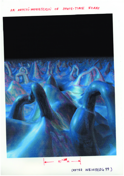
Figure 1: An artist impression of a foamy space time (S. Weinberg, Sci. Am., “A Unified Physics by 2050? (December 1999 issue))

.

The important point to notice is that in general space-time may be discrete and topologically non-trivial at Planck scales $10^{-35}~{}m$ (see fig. 1), which would in general imply Lorentz symmetry Violation (LV), and hence CPT violation (CPTV). Phenomenologically, at a macroscopic level, such LV may lead to extensions of the standard model which violate both Lorentz and CPT invariance ^?).

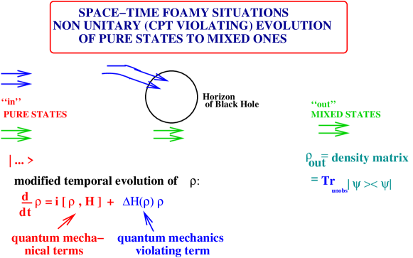
Figure 2: A basic mechanism for loss of information in a space time foamy situation.

In addition, there may be an environment of gravitational degrees of freedom (d.o.f.) inaccessible to low-energy experiments (for example non-propagating d.o.f., for which ordinary scattering is not well defined ^?)). This will lead in general to an apparent information loss for low-energy observers, who by definition can measure only propagating low-energy d.o.f. by means of scattering experiments. As a consequence, an apparent lack of unitarity and hence CPTV may arise, which is in principle independent of any LV effects. The loss of information may be understood simply by the mechanism illustrated in fig. 2. In a foamy space time there is an eternal creation and annihilation of Quantum Gravity singular fluctuations (e.g. microscopic (Planck size) black holes etc), which indeed imply that the observable space time is an open system. When matter particles pass by such fluctuations (whose life time is Planckian, of order $10^{-43}$ s), part of the particle’s quantum numbers “fall into” the horizons, and are captured by them as the microscopic horizon disappears into the foamy vacuum. This may imply the exchange of information between the observable world and the gravitational “environment” consisting of degrees of freedom inaccessible to low energy scattering experiments, such as back reaction of the absorbed matter onto the space time, recoil of the microscopic black hole etc.. In turn, such a loss of information will imply evolution of initially pure quantum-mechanical states to mixed ones for an asymptotic observer.

As a result, the asymptotic observer will have to use density matrices instead of pure states: $\rho_{out}={\rm Tr}_{\rm unobs}|out><out|=$ $ $\rho_{in}\\ \$\neq SS^{\dagger},$, with $S=e^{iHt}$ the ordinary scattering matrix. Hence, in a foamy situation the concept of the scattering matrix is replaced by that of $, introduced by Hawking ^?), which is non invertible, and in this way it quantifies the unitarity loss in the effective low-energy theory. The latter violates CPT due to a mathematical theorem by R. Wald, which we now describe ^?).

Notice that this is an effective violation, and indeed the complete theory of quantum gravity (which though is still unknown) may respect some form of CPT invariance. However, from a phenomenological point of view, this effective low-energy violation of CPT is the kind of violation we are interested in.

2.1 $ matrix and CPT Violation (CPTV)

The theorem states the following ^?): if $ $\neq S~{}S^{\dagger}$, then CPT is violated, at least in its strong form, in the sense that the CPT operator is not well defined.

For instructive purposes we shall give here an elementary proof. Suppose that CPT is conserved, then there exists a unitary, invertible CPT operator $\Theta$: $\Theta{\overline{\rho}}_{in}=\rho_{out}.$

We have $\rho_{out}=$ $ $\rho_{in}\to\Theta{\overline{\rho}}_{in}=$$ $\Theta^{-1}{\overline{\rho}}_{out}\to$ ${\overline{\rho}}_{in}=\Theta^{-1}$$ $\Theta^{-1}{\overline{\rho}}_{out}$.

But ${\overline{\rho}}_{out}=$$${\overline{\rho}}_{in}$, hence : ${\overline{\rho}}_{in}=\Theta^{-1}$$$\Theta^{-1}$ $ ${\overline{\rho}}_{in}$.

The last relation implies that $ has an inverse $${}^{-1}=\Theta^{-1}$$$\Theta^{-1}$, which however as we explained above is impossible due to information loss; hence CPT must be violated (at least in its strong form, i.e. $\Theta$ is not a well-defined operator). As I remarked before this is my preferred way of CPTV by Quantum Gravity, given that it may occur in general independently of LV and thus preferred frame approaches to quantum gravity. Indeed, I should stress at this point that the above-mentioned gravitational-environment induced decoherence may be Lorentz invariant ^?), the appropriate Lorentz transformations being slightly modified to account, for instance, for the discreteness of space time at Planck length ^?). This is an interesting topic for research, and it is by no means complete. Although the lack of an invertible scattering matrix in most of these cases implies a strong violation of CPT, nevertheless, it is interesting to demonstrate explicitly whether some form of CPT invariance holds in such cases ^?). This also includes cases with non-linear modifications of Lorentz symmetry ^?), arising from the requirement of viewing the Planck length as an invariant-observer independent proper length in space time.

It should be stressed at this stage that, if the CPT operator is not well defined, then this may lead to a whole new perspective of dealing with precision tests in meson factories. In the usual LV case of CPTV ^?), the CPT breaking is due to the fact that the CPT operator, which is well-defined as a quantum mechanical operator in this case, does not commute with the effective low-energy Hamiltonian of the matter system. This leads to a mass difference between particle and antiparticle. If, however, the CPT operator is not well defined, as is the case of the quantum-gravity induced decoherence ^?,?), then, the concept of the ‘antiparticle’ gets modified ^?). In particular, the antiparticle space is viewed as an independent subspace of the state space of the system, implying that, in the case of neutral mesons, for instance, the anti-neutral meson should not be treated as an identical particle with the corresponding meson. This leads to the possibility of novel effects associated with CPTV as regards EPR states, which may be testable at meson factories ^?).

Another reason why I prefer the CPTV via the $ matrix decoherence approach concerns a novel type of CPT violation at a global scale, which may characterize our Universe, what I would call cosmological CPT Violation, proposed in ref. ^?).

2.2 Cosmological CPTV?

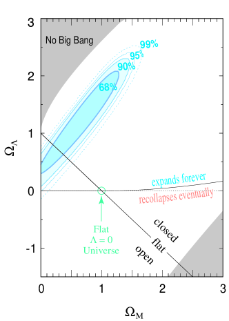
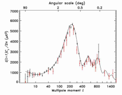
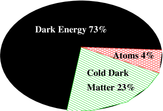
Figure 3: Recent observational evidence for Dark Energy of the Universe (upper left figure: evidence from SnIa (Ref. [17]), upper right figure: evidence from CMB measurements (Ref. [18])) and a pie graph (lower central figure) of the energy budget of our world according to these observations.

This type of CPTV is prompted by recent astrophysical Evidence for the existence of a Dark Energy component of the Universe. For instance, there is direct evidence for a current era acceleration of the Universe, based on measurements of distant supernovae SnIa ^?), which is supported also by complementary observations on Cosmic Microwave Background (CMB) anisotropies (most spectacularly by the recent data of WMAP satellite experiment) ^?).

Best fit models of the Universe from such combined data appear at presence consistent with a non-zero cosmological constant $\Lambda\neq 0$. Such a $\Lambda$-universe will eternally accelerate, as it will enter eventually an inflationary (de Sitter) phase again, in which the scale factor will diverge exponentially $a(t)\sim e^{\sqrt{\Lambda/3}t}$, $t\to\infty$. This implies that there exists a cosmological Horizon.

The existence of such Horizons implies incompatibility with a S-matrix: no proper definition of asymptotic state vectors is possible, and there is always an environment of d.o.f. crossing the horizon. This situation may be considered as dual to that of black hole, depicted in fig. 2: in that case the asymptotic observer was in the exterior of the black hole horizon, in the cosmological case the observer is inside the horizon. However, both situations are characterized by a lack of an invertible scattering matrix, hence the above-described theorem by Wald on $-matrix and CPTV applies ^?), and thus CPT is violated due to a cosmological constant $\Lambda>0$. It has been argued in ^?) that such a violation is described effective by a modified temporal evolution of matter in such a $\Lambda$-universe, which is given by

$$\partial_{t}\rho=[\rho,H]+{\cal O}(\Lambda/M_{P}^{3})\rho$$ (2)

Notice that although the order of the cosmological CPTV effects is tiny, if we accept that the Planck scale is the ordinary four-dimensional one $M_{P}\sim 10^{-19}$ GeV, and hence undetectable in direct particle physics interactions, however, as we have seen from the above considerations, they may have already been detected indirectly through the (claimed) observational evidence for a current-era acceleration of the Universe! Of course, the existence of a cosmological constant brings up other interesting challenges, such as the possibility of a proper quantization of de Sitter space as an open system, which are still unsolved.

At this point I should mention that time Relaxation models for Dark Energy (e.g. quintessence models), where eventually the vacuum energy asymptotes (in cosmological time) an equilibrium zero value are still currently compatible with the data ^?). In such cases it might be possible that there is no cosmological CPTV, since a proper S-matrix can be defined, due to lack of cosmological horizons.

From the point of view of string theory the impossibility of defining a S-matrix is very problematic, because critical strings by their very definition depend crucially on such a concept. However, this is not the case of non-critical (a kind of non equilibrium) string theory, which can accommodate in their formalism $\Lambda$ universes ^?). It is worthy of mentioning briefly that such non-critical (non-equilibrium) string theory cases are capable of accommodating models with large extra dimensions, in which the string gravitational scale $M_{s}$ is not necessarily the same as the Planck scale $M_{P}$, but it could be much smaller, e.g. in the range of a few TeV. In such cases, the CPTV effects in (2) may be much larger, since they would be suppressed by $M_{s}$ rather than $M_{P}$, and also they will be proportional to compactification volumes of the (large) extra dimensions.

It would be interesting to study further the cosmology of such models and see whether the global type of CPTV proposed in ^?), which also entails primordial CP violation of similar order, distinct from the ordinary (observed) CP violation which occurs at a later stage in the evolution of the Early Universe, may provide a realistic explanation of the initial matter-antimatter asymmetry in the Universe, and the fact that antimatter is highly suppressed today. In the standard CPT invariant approach this asymmetry is supposed to be due to ordinary CP violation. In this respect, I mention at this point that speculations about the possibility that a primordial CPTV space-time foam is responsible for the observed matter-antimatter asymmetry in the Universe have also been put forward in ^?) but from a different perspective than the one I am suggesting here. In ref. ^?) it was suggested that a novel CPTV foam-induced phase difference between a space-time spinor and its antiparticle may be responsible for the required asymmetry. Similar properties of spinors may also characterize space times with deformed Poincare symmetries ^?), which may also be viewed as candidate models of quantum gravity. In addition, other attempts to discuss the origin of such an asymmetry in the Universe have been made within the loop gravity approach to quantum gravity ^?) exploring Lorentz Violating modified dispersion relations for matter probes, especially neutrinos, which we shall discuss below.

3 Phenomenology of CPT Violation

3.1 Order of Magnitude Estimates of CPTV

Before embarking on a detailed phenomenology of CPTV it is worth asking whether such a task is really sensible, in other words how feasible it is to detect such effects in the foreseeable future. To answer this question we should present some estimates of the expected effects in some models of quantum gravity.

The order of magnitude of the CPTV effects is a highly model dependent issue, and it depends crucially on the specific way CPT is violated in a model. As we have seen cosmological (global) CPTV effects are tiny, on the other hand, quantum Gravity (local) space-time effects (e.g. space time foam) may be much larger for the following reason: Naively, Quantum Gravity (QG) has a dimensionful constant: $G_{N}\sim 1/M_{P}^{2}$, $M_{P}=10^{19}$ GeV. Hence, CPT violating and decoherening effects may be expected to be suppressed by $E^{3}/M_{P}^{2}$ , where $E$ is a typical energy scale of the low-energy probe. This would be practically undetectable in neutral mesons, but some neutrino flavour-oscillation experiments (in models where flavour symmetry is broken by quantum gravity), or some cosmic neutrino future observations might be sensitive to this order: for instance, in models with LV, one expects modified dispersion relations (m.d.r.) which could yield significant effects for ultrahigh energy ($10^{19}$ eV) $\nu$ from Gamma Ray Bursts (GRB) ^?), that could be close to observation. Also in some astrophysical cases, e.g. observations of synchrotron radiation Crab Nebula or Vela pulsar, one is able to constraint electron m.d.r. almost near this (quadratic) order ^?).

However, resummation and other effects in some theoretical models may result in much larger CPTV effects of order: $\frac{E^{2}}{M_{P}}$. This happens, e.g., in some loop gravity models ^?), or in some (non-critical) stringy models of quantum gravity involving open string excitations ^?). Such large effects are already accessible in current experiments, and as we shall see most of them are excluded by current observations. The Crab nebula synchrotron constraint ^?) for instance already excludes such effects for electrons.

3.2 Mnemonic Cubes for CPTV Phenomenology

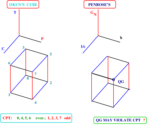
Figure 4: Mnemonic cubes for CPT Violation: Left its phenomenology. Right: its possible theoretical origin.

When CPT is violated there are many possibilities, due to the fact that C,P and T may be violated individually, with their violation independent from one another. This was emphasized by Okun ^?) some years ago, who presented a set of mnemonic rules for CPTV phenomenology, which are summarized in fig. 4. In this figure I also draw a sort of Penrose cube, indicating where the violations of CPT may come from (the diagram has to be interpreted as follows: CPTV may come from violations of special relativity (axis $1/c$), where the speed of light does not have its value, having some sort of refractive index, from departure of quantum mechanics (axis $h$), from gravity considerations where the gravitational constant departs from its value (axis $G_{N}$), or finally (and most likely) from quantum gravity considerations where all such effects may coexist.

3.3 Lorentz Violation and CPT: The Standard Model Extension (SME)

We start our discussion on phenomenology of CPT violation by considering CPTV models in which requirement (iii) of the CPT theorem is violated, that of Lorentz invariance. As mentioned previously, such a violation may be a consequence of quantum gravity fluctuations. In this case Lorentz symmetry is violated and hence CPT, but there is no necessarily quantum decoherence or unitarity loss. Phenomenologically, at low energies, such a LV will manifest itself as an extension of the standard model in (effectively) flat space times, whereby LV terms will be introduced by hand in the relevant lagrangian, with coefficients whose magnitude will be bounded by experiment ^?).

Such SME lagrangians may be viewed as the low energy limit of string theory vacua, in which some tensorial fields acquire non-trivial vacuum expectation values $<A_{\mu}>\neq 0~{},<T_{\mu_{1}\dots\mu_{n}}>\neq 0.$ This implies a spontaneous breaking of Lorentz symmetry by these (exotic) string vacua ^?).

The simplest phenomenology of CPTV in the context of SME is done by studying the physical consequences of a modified Dirac equation for charged fermion fields in SME. This is relevant for phenomenology using data from the recently produced antihydrogen factories ^?,?).

In this talk I will not cover this part in detail, as I will concentrate mainly in neutrinos within the SME context. It suffices to mention that for free hydrogen $H$ (anti-hydrogen ${\overline{H}}$) one may consider the spinor $\psi$ representing electron (positron) with charge $q=-|e|(q=|e|)$ around a proton (antiproton) of charge $-q$, which obeys the modified Dirac equation (MDE):

$$(i\gamma^{\mu}D^{\mu}-M-a_{\mu}\gamma^{\mu}-b_{\mu}\gamma_{5}\gamma^{\mu}-$$

$$-\frac{1}{2}H_{\mu\nu}\sigma^{\mu\nu}+ic_{\mu\nu}\gamma^{\mu}D^{\nu}+id_{\mu\nu}\gamma_{5}\gamma^{\mu}D^{\nu})\psi=0$$ (3)

where $D_{\mu}=\partial_{\mu}-qA_{\mu}$, $A_{\mu}=(-q/4\pi r,0)$ Coulomb potential. CPT & Lorentz violation is described by terms with parameters $a_{\mu}~{},b_{\mu}~{},$ while Lorentz violation only is described by the terms with coefficients $c_{\mu\nu}~{},d_{\mu\nu}~{},H_{\mu\nu}$.

One can perform spectroscopic tests on free and magnetically trapped molecules, looking essentially for transitions that were forbidden if CPTV and SME/MDE were not taking place. The basic conclusion is that for sensitive tests of CPT in antimatter factories frequency resolution in spectroscopic measurements has to be improved down to a range of a 1 mHz, which at present is far from being achieved ^?).

Since the presence of LV interactions in the SME affects dispersion relations of matter probes, other interesting precision tests of such extensions can be made in atomic and nuclear physics experiments, exploiting the fact of the existence of a preferred frame where observations take place. The results and the respective sensitivities of the various parameters appearing in SME are summarized in the table of figure 5, taken from the paper of ^?).

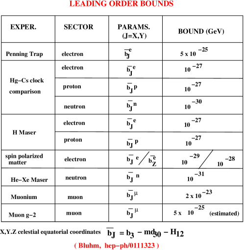
Figure 5: Sensitivities of CPTV and LV parameters appearing in SME/Modified Dirac equation for charged probes, from various atomic and nuclear physics experiments

3.4 Direct SME Tests for Neutrinos and Modified Dispersion relations (MDR)

Many LV Models of Quantum Gravity (QG) predict modified dispersion relations (MDR) for matter probes, including neutrinos $\nu$ ^?,?,?). This leads to one important class of experimental tests using $\nu$: each mass eigenstate of $\nu$ has QG deformed dispersion relations, which may, or may not, be the same for all flavours:

$$E^{2}={\vec{k}}^{2}+m_{i}^{2}+f_{i}(E,M_{qg},{\vec{k}})~{},\qquad{\rm e.g.}~{}f_{i}=\sum_{\alpha}C_{\alpha=1,2,...}{\vec{k}}^{2}(\frac{|{\vec{k}}|}{M_{qg}})^{\alpha}$$ (4)

There are stringent bounds on $f_{i}$ from oscillation experiments, as we shall discuss below.

It must be stressed that such MDR also characterize SME, although the origin of MDR in the approach of ^?,?,?) is due to an induced non-trivial microscopic curvature of space time as a result of a back reaction of matter interacting with a stringy space time foam vacuum. This is to be contrasted with the SME approach ^?), where the analysis is done exclusively on flat Minkowski space times, at a phenomenological level.

In general there are various experimental tests that can set bounds on MDR parameters, which can be summarized as follows:

(i) astrophysics tests - arrival time fluctuations for photons (model independent analysis of astrophysical GRB data ^?)

(ii) Nuclear/Atomic Physics precision measurements (clock comparison, spectroscopic tests on free and trapped molecules, quadrupole moments etc) ^?).

(iii) antihydrogen (precision spectroscopic tests on free and trapped molecules: e.g. $1S\to 2S$ forbidden transitions) ^?),

(iv) Neutrino mixing and spin-flavour conversion, a brief discussion of which we now turn to.

3.5 Neutrinos and SME

The SME formalism naturally includes the neutrino sector. Recently a SME-LV+CPTV phenomenological model for neutrinos has been given in ^?). The pertinent lagrangian terms are given by:

$${\cal L}^{\nu}_{SME}\ni\frac{1}{2}i{\overline{\psi}}_{a,L}\gamma^{\mu}D_{\mu}\psi_{a,L}-(a_{L})_{\mu ab}{\overline{\psi}}_{a,L}\gamma^{\mu}\psi_{b,L}+\frac{1}{2}i(c_{L})_{\mu\nu ab}{\overline{\psi}}_{a,L}\gamma^{\mu}D^{\nu}\psi_{b,L}$$ (5)

where $a,b$ are flavour indices. The model has (for simplicity) no $\nu$-mass differences. Notice that the presence of LV induces directional dependence (sidereal effects)!.

To analyze the physical consequences of the model, one passes to an Effective Hamiltonian ^?)

$$(H_{\rm eff})_{ab}=|{\vec{p}}|\delta_{ab}+\frac{1}{|{\vec{p}}|}((a_{L})^{\mu}p_{\mu}-(c_{L})^{\mu\nu}p_{\mu}p_{\nu})_{ab}$$ (6)

Notice that $\nu$ oscillations are now controlled by the (dimensionless) quantities $a_{L}L$ & $c_{L}LE$ where L is the oscillation length. This is to be contrasted with the conventional case, where the relevant parameter is associated necessarily with a $\nu$-mass difference $\Delta m$: $\Delta m^{2}L/E$

There is an important feature of the SME/$\nu$: despite CPTV, the oscillation probabilities are the same between $\nu$ and their antiparticles, if there are no mass differences between $\nu$ and ${\bar{\nu}}$: $P_{\nu_{x}\to\nu_{y}}=P_{{\bar{\nu}_{x}}\to{\bar{\nu}_{y}}}$.

Experimentally, it is possible to bound LV+CPTV SME parameters in the neutrino sector with high sensitivity, if we use data from high energy long baseline experiments ^?). Indeed, from the fact that there is no evidence for $\nu_{e,\mu}\to\nu_{\tau}$ oscillations, for instance, at $E\sim 100$ GeV , $L\sim 10^{-18}$ GeV^-1 we conclude that $a_{L}<10^{-18}$ GeV, $c_{L}<10^{-20}$.

Similarly for an explanation of the LSND anomaly ^?), claiming evidence for oscillations between antineutrinos (${\bar{\nu}_{\mu}}-{\bar{\nu}_{e}}$) but not for the corresponding neutrinos, a mass-squared difference of order $\Delta m^{2}=10^{-19}$ GeV${}^{2}=10^{-1}$ eV² is required, which implies that $a_{L}\sim 10^{-18}$ GeV, $c_{L}\sim 10^{-17}$. This would affect other experiments, and in fact one can easily come to the conclusion that SME/$\nu$ does not offer a good explanation for LSND, if we accept the result of that experiment as correct, which is not clear at present.

A summary of the Experimental Sensitivities for $\nu$’s SME parameters are given in the table of figure 6, taken from ^?).

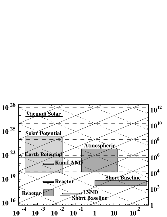
Figure 6: Approximate experimental sensitivities (from Ref. [33]). Lines of constant $L/E$ (solid), $L$ (dashed), and $LE$ (dotted) are shown, which give sensitivities to $\Delta m^{2}$, $a_{L}$, and $c_{L}$, respectively.

3.6 Lorentz non-invariance, MDR and $\nu$-oscillations

Models of quantum gravity predicting MDR of the type (4) for neutrinos ^?,?), with a leading order $E^{2}/M_{qg}$ modification, can be severely constrained by a study of the induced oscillations between neutrino flavours, as a result of the departure from the standard dispersion relations provided that the quantum-gravity foam responsible for the MDR breaks flavour symmetry, which however is not always the case ^?).

Figure 7: Shown for each experiment are (from Ref. [37]): (i) operation status, (ii) mean value of observed $\nu$ energy, (iii) the oscillation length $L$, (iv) typical $\nu$-flight distance $X$, and the ratio $\alpha=L/X$, which, in models where the foam induces $\nu$ flavour oscillations, coincides with the phenomenological parameter that controls the size of MDR effects.

This approach has been followed in ^?), where it was shown that if flavour symmetry is not protected in such MDR models, then the extra terms in (4), proportional to $E^{2}/M_{qg}$ will induce an oscillation length $L\sim 2\pi M_{qg}/(\alpha E^{2})$, where $\alpha$ is a phenomenological parameter that controls the size of the effect. This should be contrasted to the Lorentz Invariant case where $L_{\rm LI}\sim 4\pi E/\Delta m^{2}$, with $\Delta m^{2}$ the square mass difference between neutrino flavours. From a field theoretic view point, terms in MDR proportional to some positive integer power of $E^{2}/M_{qg}$ may behave as non-renormalizable operators, for instance, dimension five ^?) in the case of leading order QG effects suppressed only by a single power of $M_{qg}$.

The sensitivity of the various neutrino oscillation experiments to the parameter $\alpha$ is shown in figure 7 ^?). The conclusion from such analyses, therefore, is that, if the flavour number symmetry is not protected in such MDR foam models, then neutrino observatories and long base-line experiments should have already observed such oscillations. As remarked above, however, not all foam models that lead to such MDR predict such oscillations ^?), and hence such constraints are highly foam-model dependent.

3.7 Lorentz Non Invariance, MDR and $\nu$ spin-flavor conversion

An interesting consequence of MDR in LV quantum gravity theories is associated with modifications to the well-known phenomenon of spin-flavour conversion in $\nu$ interactions ^?). To be specific, we shall consider an example of a MDR for $\nu$ provided by a Loop Gravity approach to quantum gravity. According to such an approach, the dispersion relations for neutrinos are modified to ^?):

$$E^{2}_{\pm}=A_{p}^{2}p^{2}+\eta p^{4}\pm 2\lambda p+m^{2}$$ (7)

where $A_{p}=1+\kappa_{1}\frac{\ell_{P}}{{\cal L}},~{}\eta=\kappa_{3}\ell^{2}_{P},~{}\lambda=\kappa_{5}\frac{\ell_{P}}{2{\cal L}^{2}}$, and ${\cal L}$ is a characteristic scale of the problem, which can be either (i) ${\cal L}\sim E^{-1}$, or (ii) ${\cal L}$=constant.

It has been noted in ^?) that such a modification in the dispersion relation will affect the form of the spin-flavour conversion mechanism. Indeed, it is well known through the Mikheyev-Smirnov-Wolfenstein (MSW) effect ^?) that Weak interaction Effects of $\nu$ propagating in a medium result in an energy shift $\sqrt{2}G_{F}(2n_{e}-n_{n})$, where $n_{e}(n_{n})$’s denote electron (neutron) densities. In addition to such effects, one should also take into account the interaction of $\nu$ with external magnetic fields, $B$, via a radiatively induced magnetic moment $\mu$, corresponding to a term in the effective lagrangian: ${\cal L}_{\rm int}=\mu{\overline{\psi}}\sigma^{\mu\nu}F_{\mu\nu}\psi$, with $\psi$ the neutrino fermionic field.

According to the standard theory, the equation for evolution describing the spin-flavour conversion phenomenon due to the above-described medium and magnetic moment effects for, say, two neutrino flavours ($\nu_{e},\nu_{\mu}$) is given by:

$$i\frac{d}{dr}\left(\begin{array}[]{c}\nu_{eL}\\ \nu_{\mu L}\\ \nu_{eR}\\ \nu_{\mu R}\end{array}\right)={\cal H}\left(\begin{array}[]{c}\nu_{eL}\\ \nu_{\mu L}\\ \nu_{eR}\\ \nu_{\mu R}\end{array}\right)~{},$$ (16)

where the effective Hamiltonian ${\cal H}$ should be corrected in the loop gravity case to take into account $\lambda$-effects, associated with MDR (7) (we should notice at this stage that the above formalism refers to Dirac $\nu$; for Majorana $\nu$ one should replace: $\nu_{iL}\to\nu_{i}$, $\nu_{iR}\to{\overline{\nu}}_{i}$). Details can be found in ^?).

For our purposes we note that the Resonant Conditions for Flavour-Spin-flip are ^?):

$$\nu_{eL}\to\nu_{\mu R}:\quad 2\lambda+\frac{\Delta m^{2}}{2p}{\rm cos}2\theta-\sqrt{2}G_{F}n_{e}(r_{res})=0$$

$$\nu_{\mu L}\to\nu_{eR}:\quad 2\lambda-\frac{\Delta m^{2}}{2p}{\rm cos}2\theta-\sqrt{2}G_{F}n_{e}(r_{res})=0~{}.$$ (17)

One can use above conditions to obtain bounds for $\lambda,\kappa_{i}$ via the oscillation probabilities for spin-flavour conversion:

$$P_{\nu_{eL}\to\nu_{\mu R}}=\frac{1}{2}(1-{\rm cos}2{\tilde{\theta}}{\rm cos}2\theta)~{},$$ (18)

where ${\rm tan}2{\tilde{\theta}}(r)=\frac{4\mu B(r)E}{|\Delta m^{2}|{\rm cos}2\theta-4E\lambda+2\sqrt{2}G_{F}En_{e}(r)}$.

To obtain these bounds the author of ^?) made the following physically relevant assumptions: (a) Reasonable profiles for solar $n_{e}\sim n_{0}e^{-10.5r/R_{\odot}}$, $n_{0}=85N_{A}{\rm cm}^{-3}$. (b) Also: $\mu\sim 10^{-11}\mu_{B}$. Then, an upper bound on $\lambda$ is obtained of order: $\lambda\leq\frac{1}{2}\left(10^{-12}e^{-10.5r_{res}/R_{\odot}}{\rm eV}+\frac{|\Delta m^{2}|}{2E}\right)$.

To obtain bounds on $\kappa$ we need to distinguish two cases:

(I) ${\cal L}$=universal constant: In this case, we already know from photon dispersion tests on GRB and Active Galactic Nuclei (AGN) ^?,?) that ${\cal L}\sim 10^{-18}$ eV^-1. Then, from best-fit solar $\nu$-oscillations induced by MSW, one may use experimental values of $\Delta m^{2}$, ${\rm sin}^{2}2\theta$, and obtain the following bound on $\kappa_{i}$: $\kappa_{5}<10^{-25}$. From atmospheric oscillations, in particular LSND experiment ^?), $\nu_{\mu}\to\nu_{e}$ fits the data with: $|\Delta m^{2}|\sim eV^{2}$, ${\rm sin}^{2}2\theta\sim(0.2-3)\times 10^{-3}$, $E_{\rm max}\sim 10$ MeV, then $\kappa_{5}<10^{-17}$.

(II) ${\cal L}\sim p^{-1}$ a mobile scale: In that case, from SOLAR oscillations, with $p\sim 1-10{\rm MeV}$ one gets $\kappa_{5}={\cal O}(1-100)$, which is a natural range of values from a quantum-gravity view point. From atmospheric oscillations, for the maximum $\nu$ $E\sim 10$ MeV, and ${\cal L}\sim E^{-1}$, one obtains $\kappa_{5}\sim 10^{4}$, which is a very weak bound.

The conclusion from these considerations, therefore, is that the experimental data seem to favour case (II), at least from a naturalness point of view.

3.8 $\nu$-flavour states and modified Lorentz Invariance (MLI)

An interesting recent idea ^?), which we would like to discuss now briefly, arises from the observation of the peculiar way in which flavour $\nu$ states experience Lorentz Invariance. Indeed, neutrino flavour states are a superposition of mass eigenstates with standard dispersion relations of different mass. If one computes the expectation value of the Hamiltonian with respect to flavour states, e.g. in a simplified two-flavour scenario discussed in ^?), then one finds:

$$E_{e} = <\nu_{e}|H|\nu_{e}>=\omega_{k,1}{\rm cos}^{2}\theta+\omega_{k,2}{\rm sin}^{2}\theta~{},$$

$$E_{\mu} = <\nu_{\mu}|H|\nu_{\mu}>=\omega_{k,2}{\rm cos}^{2}\theta+\omega_{k,1}{\rm sin}^{2}\theta~{},$$ (19)

with $\theta$ the mixing angle.

One has: $H|\nu_{i}>=\omega_{i}|\nu_{i}>$, $i=1,2$, where the $\omega_{k,i}=\sqrt{{\vec{k}}^{2}+m_{i}^{2}}$ is a standard dispersion relation. However, since the sum of two square roots in not in general a square root, one concludes that flavour states do not satisfy the standard dispersion relations. In general this poses a problem, as it would naively imply the introduction of a preferred frame, due to an apparent violation of the standard linear Lorentz symmetry.

The idea of ^?), whose validity of course remains to be seen, but which I find rather intriguing, and this is why I decided to include it in this review, is to avoid using preferred frames by introducing instead non-linearly modified Lorentz transformations to account for the modified dispersion relations of the flavour states. The idea is formally similar, but physically very different, to the approach of ^?), in which, in order to ensure observer independence of the Planck length, viewed as an ordinary length in quantum gravity, and not as a universal coupling constant, one has to modify non linearly the Lorentz transformations. The result is that flavour states satisfy the following MDR:

$$E_{i}^{2}f_{i}^{2}(E_{i})-{\vec{k}}^{2}g_{i}^{2}(E_{i})=M_{i}^{2}\quad i=e,\mu$$ (20)

One can determine ^?) the $f_{i}(E_{i},\theta,m_{i}),g_{i}(E_{i},\theta,m_{i}),M_{i}(m_{i},\theta)$ by comparing with $E_{i}=E_{(}\omega_{i},m_{i})$ above ((c.f. (19)).

Then, in the spirit of ^?), one can identify the non-linear Lorentz transformation that leaves the MDR (20) invariant: $U\circ(E,{\vec{k}})=(Ef,{\vec{k}}g)$.

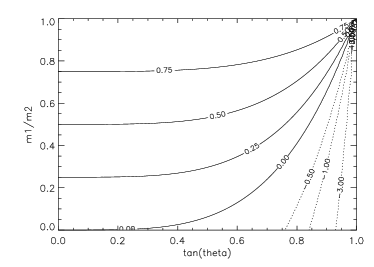
Figure 8: Left: Tail of tritium $\beta$-decay spectrum, for massless $\nu$ (solid) and for LI flavour states (dashed and dot-long-dashed). Also plotted is the preferred frame case. Right: Likelihood Contours of $M^{2}$ (in units of $m_{2}^{2}$) upon which $\beta$-decay depends (from Ref. [41]).

The interesting feature is that these ideas can be tested experimentally, e.g. in $\beta$-decay experiments: $N_{1}\to N_{2}+e^{-}+{\bar{\nu}}_{e}$, where e.g. $N_{1}=~{}^{3}{\rm H}$, $N_{2}=~{}^{3}{\rm He}$.

Energy conservation in conventional $\beta$-decay implies: $E_{N_{1}}=E_{N_{2}}+E+E_{e}$, where $E$ is the energy of $e$, which would unavoidably introduce a preferred frame. However, in the non-linear LI case for flavour states, where the use of preferred frame is avoided, this relation is modified ^?): $E_{N_{1}}=E_{N_{2}}+E+E_{e}f_{e}(E_{e})$.

These two choices are reflected in different predictions for the endpoint of the $\beta$-decay, that is the maximal kinetic energy the electron can carry (c.f. figure 8). We refer the interested reader to ^?) for further discussion on the experimental set up to test these ideas.

From the point of view of CPTV, which is our main topic of discussion here, I must mention that in such non-linearly modified Lorentz symmetry cases it is not clear what form the CPT theorem, if any, takes. This is currently under investigation ^?). In this sense, the link between CPTV and modified flavour-state dispersion relations, and therefore the interpretation of the associated experiments from this viewpoint, are issues which are not yet clear, at least to me.

3.9 CPTV for $\nu$ through QG Decoherence

So far, I have discussed the violation of CPT through the violation of Lorentz invariance. In this subsection I would like to discuss CPTV through decoherence, which is my preferred way of QG-induced CPTV. As mentioned above, in this case the mater systems are viewed as open quantum mechanical or quantum-field theoretic systems interacting with a gravitational ‘environment’, consisting of degrees of freedom inaccessible by low-energy scattering experiments. The presence of such an environment leads to modified quantum evolution, which however is not necessarily Lorentz Violating ^?). Thus, such an approach to CPTV should in principle be studied separately, and indeed it is possible for the CPTV decoherence effects to be disentangled experimentally from the LV ones, due to the frame dependence of the latter.

Before discussing the neutrino phenomenology of this type of CPTV, it is instructive to mention that the currently most sensitive particle physics probes of such a modification from quantum mechanical behavior (often called ‘quantum mechanics violation’ QMV ^?,?)) are: (i) neutral kaons and B-mesons ^?,?) and $\phi$-, B-factories (for novel CPT tests for EPR states in such factories see discussion in ^?)) (ii) ultracold (slow) neutrons in Earth’s gravitational field, and (iii) Neutrino flavour mixing, which is induced independently of masses and mass differences between neutrino species. In the discussion below we shall concentrate on this latter probe of QMV.

Quantum Gravity (QG) may induce oscillations between neutrino flavours independently of $\nu$-masses ^?,?,?,?). The basic formalism is described by a QMV evolution for the density matrix of the $\nu$:

$$\partial_{t}\rho=i[\rho,H]+\delta H\hskip-8.5pt/\hskip 2.0pt\rho$$ (21)

where ^?)

$${\delta H\hskip-8.5pt/\hskip 2.0pt}_{\alpha\beta}=\left(\begin{array}[]{cccc}0&0&0&0\\ 0&-2\alpha&-2\beta&0\\ 0&-2\beta&-2\gamma&0\\ 0&0&0&0\end{array}\right)$$

for energy and lepton number conservation, and

$${\delta H\hskip-8.5pt/\hskip 2.0pt}_{\alpha\beta}=\left(\begin{array}[]{cccc}0&0&0&0\\ 0&0&0&0\\ 0&0&-2\alpha&-2\beta\\ 0&0&-2\beta&-2\gamma\end{array}\right)$$

if energy and lepton number is violated, but flavour is conserved (the latter associated formally with the $\sigma_{1}$ Pauli matrix).

Positivity of $\rho$ requires: $\alpha,\gamma>0,\qquad\alpha\gamma>\beta^{2}$. The parameters $\alpha,\beta,\gamma$ violate CP, and CPT in general.

The relevant oscillation probabilities ^?) are given:

(A) For the flavour conserving case:

As a simplified example, consider the oscillation $\nu_{e}\to\nu_{x}$  ($x=\mu,\tau$ or sterile):

$$P_{\nu_{e}\to\nu_{x}}=\frac{1}{2}-\frac{1}{2}e^{-\gamma L}{\rm cos}^{2}2\theta_{v}-\frac{1}{2}e^{-\alpha L}{\rm sin}^{2}2\theta_{v}{\rm cos}(\frac{|m_{\nu_{1}}^{2}-m_{\nu_{2}}^{2}|}{2E_{\nu}}L)$$ (22)

Here $L$ is the oscillation length and $\theta_{v}$ is the mixing angle. Note that the mixing angle $\theta_{v}\neq 0$ if and only if the neutrinos are massless.

In the mass basis one has: $|\nu_{e}>={\rm cos}\theta_{v}|\nu_{1}>+{\rm sin}\theta_{v}|\nu_{2}>,$ $|\nu_{\mu}>=-{\rm sin}\theta_{v}|\nu_{1}>+{\rm cos}\theta_{v}|\nu_{2}>.$

From the above considerations it is clear that there flavour oscillations even in massless case, due to a non-trivial QG parameter $\gamma$, compatible with flavour conserving formalism: $<\nu_{e}|\sigma_{1}|\nu_{e}>=-<\nu_{\mu}|\sigma_{1}|\nu_{\mu}>=2{\rm sin}\theta_{v}{\rm cos}\theta_{v}.$

In the above discussion we consider only two flavours. For $n$ generations one has: $P_{\nu_{e}\to\nu_{x}}(t\to\infty)=\frac{1}{n}$.

(B) For Energy and Lepton number conserving case:

Again, we consider a two-flavour example: $\nu_{e}\to\nu_{x}$  ($x=\mu,\tau$ or sterile). The relevant oscillation probability in this case is calculated to be ^?):

$$P_{\nu_{e}\to\nu_{x}}=\frac{1}{2}{\rm sin}^{2}2\theta_{v}\left(1-e^{-(\alpha+\gamma)L}{\rm cos}(\frac{|m_{\nu_{1}}^{2}-m_{\nu_{2}}^{2}|}{2E_{\nu}}L)\right)$$ (23)

where we assumed for simplicity, and illustrative purposes, that $\alpha,\beta,\gamma\ll\frac{|m_{\nu_{1}}^{2}-m_{\nu_{2}}^{2}|}{2E_{\nu}}$.

For $n$ generations, the probability reads: $P_{\nu_{e}\to\nu_{x}}(t\to\infty)=\frac{1}{n}{\rm sin^{2}}2\theta_{v}$. The reader is invited to contrast this result with case (A) above.

One can use the results in the cases (A) and (B) to bound experimentally $\xi\equiv\{\alpha,\beta,\gamma$}. At this stage, it is worthy of mentioning that there exist two kinds of theoretical estimates/predictions for the order of magnitude of the parameters $\alpha,\beta,\gamma$: An optimistic one ^?), according to which $\xi\sim\xi_{0}(\frac{E}{\rm GeV})^{n},n=0,2,-1$, and this has a chance of being falsified in future experiments, if the effect is there, and a pessimistic one, which requires non-trivial masses for $\nu$ ^?), $\xi\sim\frac{(\Delta m^{2})^{2}}{E^{2}M_{qg}}$, ($M_{qg}\sim M_{P}\sim 10^{19}$ GeV), which is much smaller, and probably cannot be accessed by immediate future neutrino oscillation experiments.

We now mention that in some models of QG-induced decoherence, complete positivity of $\rho(t)$ for composite systems, such as $\phi$ or $B$ mesons, may be imposed ^?) (however, I must note that the necessity of this requirement, especially in a QG context where non-linear effects may be present ^?), remains to be proven). This results in an ideal Markov environment, with: $\alpha=\beta=0,\gamma>0$.

If this model is assumed for $\nu$ oscillations induced by QG decoherence ^?), then the following phenomenological parametrization can be made: $\gamma=\gamma_{0}(E/{\rm GeV})^{n}$, $n=0,2,-1$. with $E$ the neutrino energy.

Figure 9: Effects of decoherence ($\gamma=\gamma_{0}={\rm const}\neq 0$) on the distributions of lepton events as a function of the zenith angle $\vartheta$ (from Ref. [43]).

Figure 10: Best-fit scenarios for pure oscillations ($\gamma=0$) (solid line) and for pure decoherence with $\gamma\propto 1/E$ (dashed line) (from Ref. [43]).

From Atmospheric $\nu$ data one is led to the following bounds for the QG-decoherence parameter $\gamma$ (c.f. figures 9,10) ^?):

(a) $n=0$, $\gamma_{0}<3.5\times 10^{-23}$ GeV.

(b) $n=2$, $\gamma_{0}<0.9\times 10^{-27}$ GeV.

(c) $n=-1$, $\gamma_{0}<2\times 10^{-21}$ GeV.

Especially with respect to case (b) the reader is reminded that the CPLEAR bound on $\gamma$ for neutral Kaons was $\gamma<10^{-21}$ GeV ^?), i.e. the $\nu$-oscillation experiments exhibit much higher sensitivity to QG decoherence effects than neutral meson experiments.

Finally, I note that in ^?) it was remarked that very stringent bounds on $\alpha,\beta$ and $\gamma$ (in the lepton-number violating QG case) may be imposed by looking at oscillations of neutrinos from astrophysical sources (supernovae and AGN). The corresponding bounds on the $\gamma$ parameter from oscillation analysis of neutrinos from supernovae and AGN, if QG induces such oscillations, are very strong: $\gamma<10^{-40}$ GeV from Supernova1987a, using the observed constraint ^?) on the oscillation probability $P_{\nu_{e}\to\nu_{\mu},\tau}<0.2$, and $\gamma<10^{-42}$ GeV from AGN, which exhibit sensitivity to order higher than $E^{3}/M_{qg}^{2}$, with $M_{qg}\sim M_{P}\sim 10^{19}$ GeV! Of course, the bounds from AGN do not correspond to real bounds, awaiting the observation of high energy neutrinos from such astrophysical sources. In ^?) bounds have also been derived for the QG decoherence parameters by assuming that QG may induce neutrinoless double-beta decay. However, using current experimental constraints on neutrinoless double-beta decay observables ^?) one arrives at very weak bounds for the parameters $\alpha,\beta,\gamma$.

One also expects stringent bounds on decoherence parameters, but also on deformed dispersion relations, if any, for neutrinos, from future underwater neutrino telescopes, such as ANTARES ^?), and NESTOR ^?) .

3.10 CPTV and Departure from Locality for Neutrinos

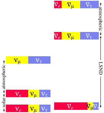
Figure 11: The CPTV spectrum proposed by Murayama-Yanagida (Ref. [53]). To explain LSND we need $m^{2}_{\nu}-m^{2}_{\bar{\nu}}\sim 0.1~{}{\rm ev}^{-2}=10^{-19}~{}{\rm GeV}^{2}$.

As a third way of violating CPT one can relax the requirement of locality. This idea has been pursued in ^?), in an attempt to present a concrete model for CPT-violation for neutrinos, with CPTV Dirac masses, in an attempt to explain the LSND anomalous results ^?). In fact the idea of invoking CPTV Dirac mass spectra for neutrinos in order to account for the LSND results without invoking a sterile neutrino is due to the authors of ^?) (see figure 11). However no concrete theoretical model was presented there.

The model lagrangian of ^?) reads:

$$S=\int d^{4}x{\bar{\psi}}i\partial_{\mu}\gamma^{\mu}\psi+\frac{im}{2\pi}\int d^{3}xdtdt^{\prime}{\bar{\psi}}(t)\frac{1}{t-t^{\prime}}\psi(t^{\prime})$$ (24)

The on shell equations (in momentum space) for the (Dirac) spinors are:

$$(p_{\mu}\gamma^{\mu}-m\epsilon(p_{0}))u_{\pm}(p)=0~{},$$ (25)

with $\epsilon(p_{0})$ the sign function, and

$$\psi_{+}(x)=u_{+}(p)e^{-ip\cdot x},\qquad p^{2}=m^{2},~{}p_{0}>0$$

$$\psi_{-}(x)=u_{-}(p)e^{-ip\cdot x},\qquad p^{2}=m^{2},~{}p_{0}<0$$ (26)

Notice that on-shell Lorentz invariance is maintained due to the presence of $(\epsilon(p_{0})$) but Locality is relaxed.

As remarked in ^?), however, the model of ^?), although respecting Lorentz symmetry on-shell, has correlation functions (which are in general off-shell quantities) that do violate Lorentz symmetry, in the sense that they transform non covariantly under Lorentz transformations.

The two-generation non-local model of ^?) seems to be marginally disfavoured by the current neutrino data, as claimed in ^?) (see figure 12).

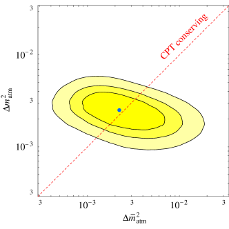
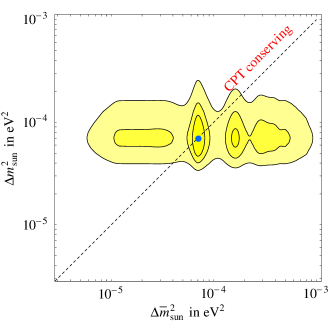
Figure 12: Left: Atmospheric $m_{\nu}-m_{\overline{\nu}}$ (68, 90, 99 %, 2 d.o.f.). Right: For solar & reactor data (68, 90, 99 %, 2 d.o.f.) (from Ref. [54]).

$$\begin{array}[]{lc|cccc}\lx@intercol\hfil\hbox{model \& no.\ of free parameters}\hfil\lx@intercol\vrule\lx@intercol&\Delta\chi^{2}&\hbox{mainly incompatible with}&\hbox{main future test}\\ \hline\cr\lx@intercol\hfil\hbox{ideal fit (no known model)}\hfil\lx@intercol\vrule\lx@intercol&0&&?\\ \Delta L=2\hbox{ decay }\bar{\mu}\to\bar{e}\bar{\nu}_{\mu}\bar{\nu}_{e}&6&12&\hbox{\sc Karmen}&\hbox{TWIST}\\ 3+1:~{}\Delta m^{2}_{\rm sterile}=\Delta m^{2}_{\rm LSND}&9&6+9?&\hbox{{\sc Bugey} + cosmology?}&\hbox{\sc MiniBoone}\\ \hbox{3 $\nu$ and CPTV~{} (no $\Delta\bar{m}^{2}_{\rm sun}$)}&10&15&\hbox{KamLAND}&\hbox{\sc KamLAND}\\ \hbox{3 $\nu$ and CPTV~{} (no $\Delta\bar{m}^{2}_{\rm atm}$)}&10&25&\hbox{SK atmospheric}&\hbox{$\bar{\nu}_{\mu}$ LBL?}\\ \hbox{normal 3 neutrinos}&5&25&\hbox{LSND}&\hbox{\sc MiniBoone}\\ 2+2:~{}\Delta m^{2}_{\rm sterile}=\Delta m^{2}_{\rm sun}&9&30&\hbox{SNO}&\hbox{SNO}\\ 2+2:~{}\Delta m^{2}_{\rm sterile}=\Delta m^{2}_{\rm atm}&9&50&\hbox{SK atmospheric}&\hbox{$\nu_{\mu}$ LBL}\\ \end{array}$$

Table 1: Interpretations of solar, atmospheric and LSND data, ordered according to the quality of their global fit. A $\Delta\chi^{2}=n^{2}$ roughly signals an incompatibility at $n$ standard deviations (from Ref. [54]).

A summary of data and interpretations of current models, including those which entail CPT violation is given in Table 1, taken from the first paper in ^?). In that paper it has also been claimed that the recent WMAP ^?) data on neutrinos seem to disfavour 3 + 1 scenaria which conserve CPT invariance. In my opinion one has to wait for future data from WMAP, before definite conclusions on this issue are reached, given that the current WMAP data are rather crude in this respect. I will not go further into a detailed discussion of this topic, as such summaries of neutrino data and their interpretations are covered by other speakers in this conference ^?).

Before closing this section, I would like to remark that most of the theoretical analyses for QG-induced CPTV in neutrinos have been done in simplified two-flavour oscillation models. Including all three generations in the formalism may lead to differences in the corresponding conclusions regarding sensitivity (or conclusions about exclusion) of the associated CPTV effects. In this respect the measurements of the mixing angle $\theta_{13}$ in the immediate future ^?), as a way of detecting generic three-flavour effects, will be very interesting. In the current phenomenology, CPT invariance is assumed for the theoretical estimates of this parameter ^?).

3.11 Four-generation $\nu$ models with CPTV

Figure 13: Upper bound (solid) on the $\nu_{\mu}\to\nu_{e}$ oscillation amplitude $4|U_{e4}|^{2}|U_{\mu 4}|^{2}$ from the GALLEX limit on $|U_{e4}|$ and the CDHSW limit on $|U_{\mu 4}|$ (90% C. L. results are used in both cases). The dot-dashed line is the 99% C. L. upper bound from Bugey and CDHSW if $CPT$ is conserved. Also shown are the expected sensitivity (dashed) of the MiniBooNE experiment and, for comparison, the allowed region (within the dotted lines) for $4|\bar{U}_{e4}|^{2}|\bar{U}_{\mu 4}|^{2}$ from a combined analysis of LSND and KARMEN data, both at the 90% C. L (from Ref. [58]).

A natural question arises at this point, concerning ($3+1$ or $2+2$) $\nu$ scenaria which violate CPT symmetry. This issue has been studied recently in ^?). These authors postulated a model for CPTV with four generations for neutrinos which leads to different flavor mixing between $\nu$, ${\bar{\nu}}$: $\nu_{a}=\sum_{i=1}^{4}U^{*}_{ai}\nu_{i},\qquad{\bar{\nu}}_{a}=\sum_{i=1}^{4}{\bar{U}}_{ai}{\bar{\nu}}_{i},$ with $U\neq{\bar{U}}$ due to CPTV. There are various cases to be studied:

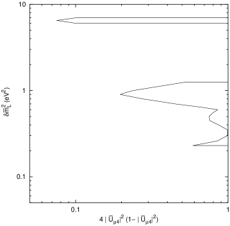
Figure 14: Lower bounds on $4|\bar{U}_{\mu 4}|^{2}(1-|\bar{U}_{\mu 4}|^{2})$ (the amplitude for atmospheric $\bar{\nu}_{\mu}$ survival at the LSND mass scale) from the Bugey limit on $\bar{\nu}_{e}$ disappearance and the $\bar{\nu}_{\mu}\to\bar{\nu}_{e}$ oscillation amplitude indicated by LSND and KARMEN (90% C. L. results are used in both cases) (from Ref. [58]).

• 3 + 1 models (see figs. 13,14): one $\nu$ mass well separated from others, sterile $\nu$ couples only to isolated state. The relevant Oscillation probabilities are: $P_{\nu_{i}\to\nu_{i}}(|U_{ij}|^{2})\neq P_{{\bar{\nu}}_{i}\to{\bar{\nu}}_{i}}(|{\bar{U}}_{ij}|^{2})$

  Experimentally one may bound $|{\bar{U}}_{e4}|$ and $U_{\mu 4}$ but there are no tight constraints for $|{\bar{U}}_{\mu 4}|$, $U_{e4}$. This is to be contrasted with (3 + 1)$\nu$ CPT conserving models where $U={\bar{U}}$. Hence (3 + 1)$\nu$ + CPTV seems still viable.

• 2 + 2 models (see fig. 15): sterile $\nu$ couples to solar and atmospheric $\nu$ oscillations. This structure is only permitted in ${\bar{\nu}}$ sector. Even with CPT Violation, however, 2+2 models are strongly disfavoured by data.

Figure 15: Constraints on sterile neutrino mixing angles $\alpha$ and $\bar{\alpha}$ from solar (solid) and atmospheric (dashed) data. The dotted line is the prediction if $CPT$ is conserved (from Ref. [58]).

4 Conclusions

From this brief exposition it becomes clear, I hope, that CPT Violation may not be an academic issue, and indeed it may characterize a theory of quantum gravity. As I discussed, neutrino physics provide stringent constraints on CPT Violation, which in some cases are much stronger than constraints from neutral meson experiments and factories. In this sense neutrinos may provide a very useful guide in our quest for a theory of Quantum Gravity. For instance, neutrino oscillation experiments provide stringent bounds on many quantum gravity models entailing Lorentz Invariance Violation. There are also plenty of low energy nuclear and atomic physics experiments which yield stringent bounds in models with Lorentz (LV) and CPT violation (notice that the frame dependence of LV effects is crucial for such high sensitivities). It is my firm opinion that neutrino factories, when built, will undoubtedly shed light on such important and fundamental issues and provide definitive answers to many questions related with LV models of quantum space time.

But, as I repeatedly stressed, Quantum Gravity may exhibit Lorentz Invariant (and hence frame independent) CPTV Decoherence. Theoretically the presence of an environment may be consistent with Lorentz Invariance ^?). This scenario is still compatible with all the existing $\nu$ data, given that the parameters of such models are highly model dependent, and thus subject at present only to constraints by experiment. It is interesting to remark, though, that, in cases where quantum gravity induces neutrino oscillations between flavours or violates lepton number, the sensitivity of experiments looking for astrophysical neutrinos from extragalactic sources may exceed the order of $1/M_{P}^{2}$ in the respective figures of merit, and thus is far more superior than the sensitivities of meson factories and nuclear and atomic physics experiments, viewed as probes of quantum mechanics .

Clearly much more work, both theoretical and experimental, is needed before definite conclusions are reached. Nevertheless, I personally believe that research on neutrinos could soon make important contributions to our fundamental quest for understanding the quantum structure of space time. Neutrino research certainly constitutes a very interesting area of fundamental physics, which will provide fruitful collaboration between astrophysics and particle physics, and which, apart from the exciting possibility of non-zero neutrino masses, may still hide even further surprises waiting to be discovered in the near future.

5 Acknowledgements

It is a real pleasure to thank Prof. M. Baldo-Ceolin for the invitation and for organizing this very successful and thought-stimulating meeting. I would also like to acknowledge informative discussions with G. Barenboim on Early Universe neutrino physics, J. Bernabeu and J. Papavassiliou on CPT phenomenology, and G. Tzanakos on the MINOS experiment and prospects for detection of generic three-flavour $\nu$ effects. This work is partly supported by the European Union (contract HPRN-CT-2000-00152).

References

- [1] G. Lüders, Det. Kong. Danske Videnskabernes Selskab, Mat.-Fys. Medd. No 5 (1954) 28; Annals Phys. 2 (1957) 1 [Annals Phys. 281 (2000) 1004]. W. Pauli, in Niels Bohr and the Development of Physics (Mc Graw-Hill, New York, 1955), p. 30.
- [2] see: A. Zichichi, in John Bell and the ten challenges of subnuclear physics (Bertlmann, R.A. (ed.) et al.: Quantum unspeakables, 2000), p. 429.
- [3] R. Jost, Helv. Phys. Acta 30 (1957), 409; also in Theoretical Physics in the Twentieth Century (Interscience, New York, 1960).
- [4] R.F. Streater and A.S. Wightman, PCT, Spin & Statistics, and All That (Benjamin, New York, 1964).
- [5] O. W. Greenberg, arXiv:hep-ph/0309309; O. W. Greenberg, Phys. Rev. Lett. 89 (2002) 231602 [arXiv:hep-ph/0201258].
- [6] see for instance: J. A. Wheeler and K. Ford, Geons, Black Holes and Quantum Foam: A Life in Physics (Norton, New York, 1998); S. W. Hawking, Commun. Math. Phys. 87 (1982) 395.
- [7] J. R. Ellis, J. S. Hagelin, D. V. Nanopoulos and M. Srednicki, Nucl. Phys. B241 (1984) 381.
- [8] J. R. Ellis, N. E. Mavromatos and D. V. Nanopoulos, Phys. Lett. B293 (1992) 142 [arXiv:hep-ph/9207268]; Int. J. Mod. Phys. A11 (1996) 1489 [arXiv:hep-th/9212057]; J. R. Ellis, J. L. Lopez, N. E. Mavromatos and D. V. Nanopoulos, Phys. Rev. D53 (1996) 3846 [arXiv:hep-ph/9505340].
- [9] A. Kostelecky, arXiv:hep-th/0312310 and references therein.
- [10] R. M. Wald, Phys. Rev. D21 (1980) 2742.
- [11] G. J. Milburn, arXiv:gr-qc/0308021;
- [12] F. Dowker, J. Henson and R. D. Sorkin, arXiv:gr-qc/0311055.
- [13] N. E. Mavromatos and Alison Waldron, in preparation.
- [14] G. Amelino-Camelia, Int. J. Mod. Phys. D11 (2002) 35 [arXiv:gr-qc/0012051]; J. Magueijo and L. Smolin, Phys. Rev. Lett. 88 (2002) 190403 [arXiv:hep-th/0112090].
- [15] J. Bernabeu, N. E. Mavromatos and J. Papavassiliou, arXiv:hep-ph/0310180, Phys. Rev. Lett. to appear.
- [16] N. E. Mavromatos, arXiv:hep-ph/0309221, Proc. Beyond the Desert 2003 (Castle Ringberg, Tegernsee, Germany, 9-14 Jun 2003) in press.
- [17] B. P. Schmidt et al., Astrophys. J. 507 (1998) 46 [arXiv:astro-ph/9805200]; S. Perlmutter et al. [Supernova Cosmology Project Coll.], Astrophys. J. 517 (1999) 565 [arXiv:astro-ph/9812133].
- [18] C. L. Bennett et al., Astrophys. J. Suppl. 148 (2003) 1 [arXiv:astro-ph/0302207]; D. N. Spergel et al., Astrophys. J. Suppl. 148 (2003) 175 [arXiv:astro-ph/0302209].
- [19] see talk by S. Bludman, these proceedings and references therein (http://axpd24.pd.infn.it/NO-VE/prog-NOVE.html).
- [20] D. V. Ahluwalia and M. Kirchbach, Int. J. Mod. Phys. D10 (2001) 811 [arXiv:astro-ph/0107246]. See also: D. V. Ahluwalia-Khalilova, arXiv:hep-ph/0305336.
- [21] A. Agostini, arXiv:hep-th/0312305 and references therein.
- [22] G. Lambiase and P. Singh, Phys. Lett. B565 (2003) 27 [arXiv:gr-qc/0304051].
- [23] J. R. Ellis, N. E. Mavromatos, D. V. Nanopoulos and G. Volkov, Gen. Rel. Grav. 32 (2000) 1777 [arXiv:gr-qc/9911055].
- [24] J. R. Ellis, N. E. Mavromatos, D. V. Nanopoulos and A. S. Sakharov, arXiv:astro-ph/0309144, Astroparticle Phys. in press.
- [25] see for instance L. Smolin, arXiv:hep-th/0303185, and references therein.
- [26] T. Jacobson, S. Liberati and D. Mattingly, Nature 424 (2003) 1019 [arXiv:astro-ph/0212190].
- [27] L. B. Okun, arXiv:hep-ph/0210052.
- [28] A. Amorreti et al. [ATHENA Coll.], Nature 419 (2002) 456; G. Gabrielse et al. [ATRAP Coll.], Phys. Rev. Lett. 89 (2002) 213401.
- [29] N. E. Mavromatos, Nucl. Instrum. Meth. B214 (2004) 1 [arXiv:hep-ph/0305215] and references therein. See also: http://ad3-proj-leap03.web.cern.ch/ad3-proj-leap03/
- [30] R. Bluhm, arXiv:hep-ph/0308281; arXiv:hep-ph/0111323, and references therein.
- [31] G. Amelino-Camelia, J. R. Ellis, N. E. Mavromatos and D. V. Nanopoulos, Int. J. Mod. Phys. A12 (1997) 607 [arXiv:hep-th/9605211]; G. Amelino-Camelia, J. R. Ellis, N. E. Mavromatos, D. V. Nanopoulos and S. Sarkar, Nature 393 (1998) 763 [arXiv:astro-ph/9712103].
- [32] J. R. Ellis, K. Farakos, N. E. Mavromatos, V. A. Mitsou and D. V. Nanopoulos, Astrophys. J. 535 (2000) 139 [arXiv:astro-ph/9907340]; J. R. Ellis, N. E. Mavromatos, D. V. Nanopoulos and A. S. Sakharov, Astron. Astrophys. 402 (2003) 409 [arXiv:astro-ph/0210124].
- [33] A. V. Kostelecky and M. Mewes, arXiv:hep-ph/0308300; arXiv:hep-ph/0309025.
- [34] see for instance: G. Drexlin, Nucl. Phys. Proc. Suppl. 118 (2003) 146, and references therein.
- [35] J. Alfaro, H. A. Morales-Tecotl and L. F. Urrutia, Phys. Rev. Lett. 84 (2000) 2318 [arXiv:gr-qc/9909079].
- [36] J. R. Ellis, N. E. Mavromatos and D. V. Nanopoulos, Phys. Rev. D65 (2002) 064007 [arXiv:astro-ph/0108295].
- [37] R. Brustein, D. Eichler and S. Foffa, Phys. Rev. D65 (2002) 105006 [arXiv:hep-ph/0106309].
- [38] R. C. Myers and M. Pospelov, Phys. Rev. Lett. 90 (2003) 211601 [arXiv:hep-ph/0301124].
- [39] G. Lambiase, Class. Quant. Grav. 20 (2003) 4213 [arXiv:gr-qc/0302053].
- [40] L. Wolfenstein, Phys. Rev. D17 (1978) 2369. Phys. Rev. D20 (1979) 2634; S. P. Mikheev and A. Y. Smirnov, Sov. J. Nucl. Phys. 42 (1985) 913 [Yad. Fiz. 42 (1985) 1441];
- [41] M. Blasone, J. Magueijo and P. Pires-Pacheco, arXiv:hep-ph/0307205.
- [42] Y. Liu, L. z. Hu and M. L. Ge, Phys. Rev. D56 (1997) 6648; C. H. Chang, W. S. Dai, X. Q. Li, Y. Liu, F. C. Ma and Z. j. Tao, Phys. Rev. D60 (1999) 033006 [arXiv:hep-ph/9809371].
- [43] E. Lisi, A. Marrone and D. Montanino, Phys. Rev. Lett. 85 (2000) 1166 [arXiv:hep-ph/0002053].
- [44] F. Benatti and R. Floreanini, Phys. Rev. D64 (2001) 085015 [arXiv:hep-ph/0105303].
- [45] H. V. Klapdor-Kleingrothaus, H. Paes and U. Sarkar, Eur. Phys. J. A8 (2000) 577 [arXiv:hep-ph/0004123].
- [46] S. L. Adler, Phys. Rev. D62 (2000) 117901 [arXiv:hep-ph/0005220].
- [47] R. Adler et al. [CPLEAR Coll.], Phys. Lett. B 364 (1995) 239 [arXiv:hep-ex/9511001].
- [48] A. Y. Smirnov, D. N. Spergel and J. N. Bahcall, Phys. Rev. D49 (1994) 1389.
- [49] [Heidelberg Moscow Coll.], Phys. Rev. Lett 83 (1999) 41 ; H. V. Klapdor-Kleingrothaus et al., hep-ph/99010205 [on behalf of GENIUS Coll.].
- [50] G. D. Hallewell [ANTARES Coll.], Nucl. Instrum. Meth. A502 (2003) 138, and references therein.
- [51] S. E. Tzamarias [NESTOR Coll.], Nucl. Instrum. Meth. A502 (2003) 150, and references therein.
- [52] G. Barenboim and J. Lykken, Phys. Lett. B 554 (2003) 73 [arXiv:hep-ph/0210411] and references therein.
- [53] H. Murayama and T. Yanagida, Phys. Lett. B 520 (2001) 263 [arXiv:hep-ph/0010178].
- [54] A. Strumia, Phys. Lett. B 539 (2002) 91 [arXiv:hep-ph/0201134]; arXiv:hep-ex/0304039.
- [55] see for instance: A. Smirnov, these proceedings and references therein (http://axpd24.pd.infn.it/NO-VE/prog-NOVE.html).
- [56] K. Lang [on behalf of MINOS Coll.] Int. J. Mod. Phys. A18 (2003) 3857, and references therein.
- [57] see talk by: M. Lindner, these proceedings and references therein (http://axpd24.pd.infn.it/NO-VE/prog-NOVE.html).
- [58] V. Barger, D. Marfatia and K. Whisnant, Phys. Lett. B 576 (2003) 303. [arXiv:hep-ph/0308299].