ASTROPHYSICAL OBSERVATIONS OF EARLY UNIVERSE PHASE TRANSITIONS

1 Review of CMBR Correlations

Until about 380,000 years after the “big bang” the temperature of the universe was higher than atomic binding energies and atoms were ionized. At that time the temperature fell to about 0.25 ev, electrons bound to atomic nuclei, and the scattering of electromagnetic radiation from the early periods of the universe almost ceased. We now observe this radiation after this last scattering, called the Cosmic Microwave Background Radiation (CMBR).

1.1 Evolution of the Early Universe

During the period before the last scattering there were many important astrophysical processes. For todays purposes we classify them by the time, t, and temperature, T, at the time as:

Very early: inflation, strings, textures, etc.

t$\simeq 10^{-11}s$; T $\simeq 100GeV\simeq$ Higgs Mass: The early universe Electroweak Phase Transition (EWPT)

t$\simeq 10^{-5}s$; T $\simeq$ 300 MeV: the early universe QCD Chiral Phase Transition, or quark hadron phase transitiion(QHPT) (at T $\simeq$ 150 MeV).

t$\simeq$ 380,000 years: Last Scattering, CMBR free, carries information about cosmological processes in the early universe.

Our main interest in the present work is to to find if the EW or QH phase transitions can produce observable effects in the CMBR radiation or other astrophysical observations.

1.2 Formalism for CMBR Correlatons

The starting point is to make a T=Temperature map using blackbody spectrum with the microwave telescope in the $\hat{n}$ direction. Expanding T($\hat{n}$) in spherical harmonics

$$\frac{T(\hat{n})}{T_{0}}=1+\sum_{lm}a^{T}_{lm}Y_{lm}(\hat{n})\;.$$ (1)

From $T_{0}=2.73K^{o}\rightarrow$ we know that the big bang occured $\sim$ 14 billion years ago. The temperature fluctuations, $\Delta T$, are given by $a^{T}_{lm}$. They are random: $<a^{T}_{lm}>=0$.

1.2.1 Temperature and Polarization Correlations

The CMBR correlations are defined in terms of the Stokes parameters for a plane electromagnetic wave (see, e.g., Jackson’s text on Classical Electrodynamics): $I\sim$ intensity or T, Q and U $\sim$ E and B type of polarization, and V $\sim$ circular polarization. The Stokes parameter V does not have to be considered. The diagonal correlations, with $<a^{T}_{l^{\prime}m^{\prime}}a^{T}_{lm}>=C^{TT}_{l}\delta_{ll^{\prime}}\delta_{mm^{\prime}}$, are

$$<\frac{\Delta T(\hat{q}_{1})}{T_{0}}\frac{\Delta T(\hat{q}_{2})}{T_{0}}> = \sum_{l}\frac{2l+1}{4\pi}C^{TT}_{l}P_{l}(cos\alpha)$$ (2)

$$<\frac{Q(\hat{q}_{1})}{T_{0}}\frac{Q(\hat{q}_{2})}{T_{0}}> = \sum_{l}\frac{2l+1}{4\pi}C^{EE}_{l}P_{l}(cos\alpha)$$ (3)

$$<\frac{U(\hat{q}_{1})}{T_{0}}\frac{U(\hat{q}_{2})}{T_{0}}> = \sum_{l}\frac{2l+1}{4\pi}C^{BB}_{l}P_{l}(cos\alpha)\;.$$ (4)

The Temperature and polarizations correlations, $C^{TT}_{l},C^{EE}_{l},C^{BB}_{l}$, as well as the cross correlations, are the key observations of CMBR experiments.

1.2.2 Cosmology and CMBR Measurements

Consider some cosmological event, such as inflation, EWPT, or QHPT. These processes can give rise to seeds. One must evolve these seeds to the last scattering time. We briefly review this, using the Hu-White[1] formalism

Let us defines the vector $\vec{T}(\Theta,Q+iU,Q-iU),\Theta=\Delta T/T$, with the three components constructed from the Stokes parameters. The Boltzman equation to evolve to last scattering time is

$\frac{d\vec{T}}{d\eta}=C[T]+G[h_{\mu\nu}]$
with $\eta=t/a(t)$ = conformal time, a(t)= cosmic scale, $g_{\mu\nu}=a(t)^{2}[g_{\mu\nu}^{0}+h_{\mu\nu}$ = metric tensor, $h_{\mu\nu}\rightarrow$ metric perturbations, $C[T]\rightarrow$ Compton scattering, and $G[h_{\mu\nu}]\rightarrow$ gravitational (metric) fluctuations.

To find correlations $C^{TT}_{l},C^{EE}_{l},C^{BB}_{l}$ one expands in angular modes, inserts $\Theta$, Q, and U in the Boltzman equation, and does the angular integrals. The Boltzman equation takes seed from time of cosmological events to last scattering time to obtain $C^{XY}_{l}$ The solutions to Boltzman Eq. at conformal time $\eta_{0}$ for the angular projections of the Stokes functions are

$$\frac{\Theta^{m}_{l}(\eta_{0},\vec{k})}{2l+1} = \int_{0}^{\eta_{0}}d\eta\frac{g(\eta_{0},\eta)}{\dot{\tau}(\eta)}\sum_{l^{\prime}}S^{m}_{l^{\prime}}j^{l^{\prime},m}_{l}[k(\eta_{0}-\eta)]\;,$$ (5)

$$\frac{B^{m}_{l}(\eta_{0},\vec{k})}{2l+1} = -\sqrt{6}\int_{0}^{\eta_{0}}d\eta g(\tau_{0}(\eta),\tau(\eta))P^{m}\beta^{m}_{l}[k(\eta_{0}-\eta)]\;,$$ (6)

and a similar expression for $E^{m}_{l}$, with $j^{l^{\prime},m}_{l},\beta^{m}_{l}$ related to Bessel functions, with $\tau(\eta)$ the optical depth, $g(\tau_{0},\tau)$ is the visibility function,and $S^{m}_{l}(\eta),P^{m}(\eta)$ are the sources of T,E,B fluctuations.

$C^{X,X^{\prime}}$ fluctuations are obtained from integrals over products of $\Theta^{m}_{l},E^{m}_{l},B^{m}_{l}$ at $\eta_{0}$.

1.3 CMBR Measurements, Very Early Univerwse Cosmological Predictions

A recent history of CMBR measurements after COBE, $l\leq 200$ is:

BOOMERANG Baloon telescope, 1998, A.E. Lang et al, Phys. Rev. D63 (2001)04200, Resolution 10 arcmin. $50\leq l\leq 800$

MAXIMA Baloon telescope, 1998, S. Hanney et al, Ap.J. Lett. 545 (’00)5. Resolution 10 arcmin $35\leq l\leq 785$

ACBAR Uses VIPER (CMU), Antartica

DASI Interferometer, Antartica

WMAP Wilkinson Microwave Anisotropy Probe, C.L. Bennet et.al., Astrophys. J. Suppl. 148 (2003) 1.

The first important thing that we learn from CMBR measurements in recent years is that the First (acoustic) peak at $l\simeq 200\rightarrow\Omega\simeq 1.0$, FLAT UNIVERSE. From the recent WMAP experiment TE polarizations have been seen. There are prospects that BB correlations, which are most important for our present work (as we discuss in the next section), will be observed

As mentioned above, cosmological theorists must find effects that can observed. Predictions of CMBR correlations from defect models and inflation models have been made (see [2, 3]). For our present purposes the most important results are for BB polarization, which we discuss in the next section.

2 QCD Phase Transition

Starting from the QCD Lagrangian

$$\mathcal{L}^{glue} = -\frac{1}{4}G\cdot G$$ (7)

$$G_{\mu\nu}^{n} = \partial_{\mu}A_{\nu}-\partial_{\nu}A_{\mu}-ig[A_{\mu},A_{\nu}]$$

$$A_{\mu} = A_{\mu}^{n}\lambda^{n}/2$$ (8)

with $\lambda^{n}$ the eight SU(3) Gell-Mann matrices, use the instanton model, which gives for the QCD gluonic Lagrangian for instantons of size $\rho$

$$\frac{1}{4}G^{inst}\cdot G^{inst} = 48\frac{\rho^{4}}{(x^{2}+\rho^{2})^{4}}\;.$$ (9)

2.1 Bubble Surface Tension in Instanton-Like Model

In order to investigate bubble collisions that could lead to observations one must develope a good model for the bubble wall. For the QHPT we take guidance from the instanton model[4] to calculate the surface tension[5]. In the instanton model, a SU(2) Euclidean space model,the energy density $T^{00}$ = 0. In Minkowski space one finds

$$T^{00(inst)} = 3(2)^{5}\big{(}\frac{\rho}{x^{2}+\rho^{2}}\big{)}^{4}\;.$$ (10)

The bubble wall surface tension for one instanton is

$$\sigma^{inst}(T=0) = \int dxT^{00}(x,0,0)$$ (11)

$$= \frac{30\pi}{\rho^{3}}\;.$$

Use lattice gauge picture-double peak and the $n(T_{c})=0.5n(T=0)$ = 0.0004 from the liquid instanton model[6] we find

$$\sigma(T_{c})^{instanton\;model} = .013T_{c}^{3}$$ (12)

$$\sigma(lattice) \simeq .015T_{c}^{3}\;,$$

quite good agreement with the lattice[7] calculation.

2.2 Collisions of Instanton-like Bubbles

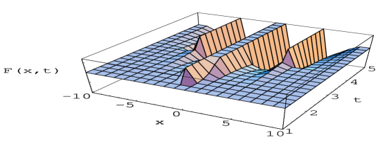
Figure 1: F(x,t) for the two bubbles with instanton-like form

From the classical theory of bubble collisions, when two bubbles collide an interior wall with the same surface tension as the original bubble walls is formed. For the QHPT the our picture would have a short-lived QCD gluonic instanton-like wall. To test this we[8] look for solutions to the equations of motion with the purely gluonic Lagrangian, Eq.( 7) in 1+1 Minkowski space, with the gauge condition $\partial_{\mu}A^{a}_{\mu}=0$. I will give a very brief description as the details of this are discussed by Mikkel Johnson in his talk at this Workshop.

Using the instanton-like ansatz, with $\eta_{a\mu\nu}$ defined in Ref.  [4],

$$A^{a}_{\mu}(x) = \frac{2}{g}\eta_{a\mu\nu}x^{\nu}F(x^{2})\equiv\eta_{a\mu\nu}W^{\nu}\;.$$ (13)

The equation of motion for F is

$$\partial^{2}F = -\frac{2}{x}\partial_{x}F-12F^{2}+8(x^{2}-t^{2})F^{3}\;.$$ (14)

Typical results showing the interior gluonic wall forming are shown in Fig.1. This is the physical basis for our magnetic wall and CMBR polarization correlations discussed in the next section.

3 QHPT, Magnetic Walls, and CMBR Correlations

In this section we discuss the magnetic wall which would form from QCD bubble collisions during the QHPT, and how this could provide the seed for observable BB polarization correlations in the CMBR[9] Starting from the electromagnetic interaction

$${\cal L}^{int} = -e\bar{\Psi}\gamma^{\mu}A^{em}_{\mu}\Psi,$$ (15)

where $\Psi$ is the nucleon field operator, in Ref [9] a magnetic wall was derived with the form

$${\bf B}_{W}({\bf x}) = B_{W}e^{-b^{2}(x^{2}+y^{2})}e^{-M_{n}^{2}z^{2}}\;,$$ (16)

$b^{-1}=d_{H}\simeq$ few km, $M_{n}^{-1}\simeq 0.2fm$, and $B_{W}\simeq\frac{3e}{14\pi}\Lambda_{QCD}\simeq 10^{17}$ Gauss within the wall. The compton scattering from this wall provides the seed, $P^{2}$ in Eq.(6), from which the solution of the Boltzman equation and the formalism described in Sec.I gives for the BB polarization correlation:

$$C^{BB}_{l} \simeq 4.25\times 10^{-8}l^{2}$$ (17)

This is illustrated in Fig.2.

Note that for large $l$ we find BB CMBR correlations which can be tested as they are different from very early universe models.

In Ref [9] a calculation of metric fluctuations the $C^{BB}_{l}$ arising from metric fluctuation, gravity wave effects were also estimated.

4 Electroweak Phase Transition

At a time t$\simeq 10^{11}$s T$\simeq$ 100 GeV. At that time the EWPT occured, and the Higgs and gauge bosons acquired their masses. In recent years it has been recognized[10] that with the standard Weinberg-Salam Model at finite T there is no first order phase transition, and no EW bubble formation. Although even a crossover EWPT is important for baryogenesis, there would be no observable cosmological effects.

With a minimal supersymmetric model a first order EWPT is possible. See, e.g., Ref [11]. After integrating out the second Higgs and all supersymmetric partners except the stop, the Lagrangian is of the form

$${\cal L}^{EW} = {\cal L}^{WS}+{\cal L}^{stop}$$

$${\cal L}^{stop} = |D_{\mu}\Phi_{t}|^{2}+m_{t}^{2}|\Phi_{t}|^{2}$$

$$D_{\mu} = i\partial_{\mu}-\frac{g}{2}\tau\cdot W_{\mu}-\frac{g^{\prime}}{2}B_{\mu}\,,$$ (18)

where the $W^{i},W^{3},B$, with i = (1,2),are the EW gauge fields, and $\Phi_{t}$ is the Stop field, with $\Phi_{L},\Phi_{R}$. The e.o.m. are obtained from $\delta\int d^{4}{\cal L}^{EW}=0$ The solution of the e.o.m.is a PISETAL project (Choi, Henley, Hwang, Johnson, Walawalkar,and Kisslinger). Our main objective is to derive the magnetic fields generated in EWPT bubble collisions to find seeds for galactic and extra-galactic magnetic fields, an unsolved problem.

5 Conclusions

The QCD chiral phase transition might lead to large-scale gluonic walls.

If gluonic walls are metastable, magnetic walls would form.

Large-scale magnetic walls would lead to observable CMBR polarization correlations and density fluctuations for $l>1000$.

For the electroweak phase transition one needs the MSSM or other extensions of the WSM. Observable Magnetic fields in galaxy structure might result.

^† This work was supported in part by NSF grant PHY-00070888.

References

- [1] W. Hu and M. White, Phys. Rev. D 56, 596 (1997).
- [2] U. Seljak, U-L. Pen and N. Turnok, Phys. Rev. Lett.79, 1615 (1997).
- [3] M. Kamionkowski and A. Kosowsky, Phys. Rev. D 57, 685 (1998).
- [4] A.A. Belavin et. al., Phys. Lett. 59, 85 (1975); G. ’t Hooft, Phys. Rev. 14, 3432 (1976).
- [5] L.S. Kisslinger, hep-ph/0202159 (2002).
- [6] T. Schaffer and E.V. Shuryak, Phys. Rev. Rev Mod. Phys. 70, 323 (1998).
- [7] B. Beinlich, F. Karsch and A. Peikert, Phys. Lett. B 390, 268 (1997).
- [8] M.B. Johnson, H-M. Choi and L.S. Kisslinger, Nucl. Phys. bf A 729, 729 (2003).
- [9] L.S. Kisslinger, Phys. Rev. D 68, 043516 (2003).
- [10] K. Kajantie, et. al. Phys. Rev. Lett.14, 2887 (1996).
- [11] M. Laine, Nuc. Phys B481, 43 (1996).