2004 Review of Light Cone Field Theory
PACS Indices: 11.30.Cp,12.38.Lg,12.39.Ki,13.40.Gp,13.25.Hw
† email: kissling@andrew.cmu.edu
CONTENTS
1 Introduction
2 Light Cone Quantum Mechanics
3 Light Cone Field Theory
4 B-S Equation in a Light Cone Representation and Pion Form Factor
5 Light Cone Representation of the Quark Schwinger-Dyson Equation
6 Deeply Virtual Compton Scattering and Skewed Parton Distributions
7 Rare Decays
8 Meson light Cone Wave Functions
9 Factorization and Experimental Study of Light Cone Wave Functions
1 Introduction
Light cone quantization was introduced by Dirac in his exploration[1] of possible representations of the Poincar Group for relativistic formulations of quantum mechanics. The most obvious application in nuclear and particle physics is to high momentum transfer processes for hadrons and nuclei, since in a light cone representation a diagonal Lorenz boost operator can be defined, while in the standard instant form representation Lorentz boosts of bound systems are difficult to formulate.
There have been several reviews of light cone quantization for Hamiltonian Dynamics with various applications to bound states (see Ref.[2] for references) and the light cone representations of bound states in supersymmetric theories[3]. The light cone community holds an annual meeting, and this review is based in part on developments in this area presented and discussed at the International Workshop Light cone 2002[4]
The light cone formulation of Quantum Chromodynamics (QCD) field theory, the presently accepted theory of strong interactions, is particularly important, since only by treating processes from low momentum transfer to high momentum transfer can one explore the transition from nonperturbative to perturbative regions, which is still an unsolved problem. Light cone formulations are important for such studies. E.g., in one of the early applications of light cone formulations to form factors it was shown[5] that with a model that predicts that nonperturbative processes dominate the pion form factor until momentum transfer , and that at 5 GeV2 perturbative QCD theory might begin to be applicable, it was found in an instant form treatment of the same model[6] that only at much higher values of can perturbative QCD be used. Light cone treatments of the pion form factor are reviewed below.
In the present review we shall center on applications to processes involving either high momentum transfer or both high and low momentum transfer.
2 Light Cone Quantum Mechanics
In this section we review the light cone formulation of relativistic quantum mechanics. Quantum mechanics is based on states and operators, which must tranform correctly under Lorentz transformations in a relativistic theory. The Poincar group of translations, rotations, and Lorentz transformations in the standard instant form has serious problems for Lorentz transformations, and as we shall see this problem is much less serious in the light cone representation.
These problems are more serious in field theories, which we review in the following section, and a number of the concepts which arise in quantum mechanics apply with modifications in field theories.
2.1 Lorentz Transformations and the Poincar Group
The invariant distance, is defined in terms of the four position, by the metric tensor, , by
| (1) |
where the Greek indices run (1,…4). An inhomogeneous Lorentz transformation of the position 4-vector is given by
| (2) |
where is a constant and is the constant Lorentz matrix, which satisfies
| (3) |
The ten generators of infinitesimal Lorentz transformations are:
| (4) | |||||
with .
These ten operators form the Poincar group, which satisfy the the commutation rules (Poincar Algebra)
| (5) | |||||
In the next two subsections we consider the instant form and light cone representations.
2.1.1 Instant Form for Dirac Particles
The instant form is the one commonly used in relativistic quantum mechanics:
| (6) | |||||
| (7) |
with = (0,1,2,3).
Let us first consider a free Dirac Particle. The ten generators (c= h/ =1) at t=0 are
| (8) | |||||
where . and are the usual momentum and internal spin operators. Wave functions transform under the group by
| (9) | |||||
| (10) | |||||
| (11) |
with a rotation of about the axis and a Lorentz boost of tanh = v in the direction.
For a system of interacting fermions in the instant form the boost operator contains the interaction potential. There has been a great deal of literature on this subject, starting with Foldy’s expansion in c-2 [7]. We do not discuss this further here.
2.1.2 Light Cone Form for Dirac Particles
The light cone form is defined by
| (12) | |||||
| (17) |
The Poincar generators are
| (18) | |||||
momentum operators and
| (23) |
angular momentum operators, with
| (24) | |||||
In this light cone form one can choose seven generators to be independent of the interaction (often called “good” generators), such as (see [1, 8, 9])
| (25) |
so that one can carry out a Lorentz boost in one direction without involving interactions. This is also true for field theory, as we shall see, and is most significant, since interactions generally produce particles. The other three generators (the “bad” generators)
| (26) |
contain the interactions. Therefore, although a boost in the z direction is interaction free, rotations about the x and y axes are not; therefore prescriptions for total angular momentum for composite states are needed. See, e.g., Ref[10].
2.2 Light Front Hamiltonian Dynamics
One method for constructing a relativistic quantum theory for interacting particles with an interaction-independent Lorentz boost follows the Bakamjian-Thomas idea[11] of using M, the invariant mass operator. See Ref.[12] for a review and references.
The energy operator in this method is
| (27) |
The method of obtaining solutions to the Hamiltonian eigenvalue problem, with the Hamiltonian operator containing the interactions,
| (28) |
for the states and wave functions by a Fock state expansion is discussed in detail in Ref.[2], with discussion of applications to QCD and QED. There is an extensive discussion of applications for relativistic corrections in nuclear physics in Ref.[12]. In the present review we concentrate on applications of light cone field theory, which is discussed next.
3 Light Cone Field Theory
In this section we review the light cone formalism for quantum field theory. One of our main objectives is to discuss the derivation of the ten Poincar generators, with an interaction-free Lorentz boost operator. First we review the instant form procedure for deriving the Poincar generators.
3.1 Poincar Generators in Instant Form Field Theory
The starting point in a quantum field theory is the Lagrangian density, , with the fields , the conjugate momenta , and the commutation rules of the fields,
| (29) |
The Poincar generators are obtained from the energy momentum tensor, which can be derived from
| (30) |
E.g., the Lagrangian density for pure glue QCD is
| (31) |
with
| (32) | |||||
where are the eight SU(3) Gell-Mann matrices, . The corresponding energy momentum tensor is given by
| (33) |
The momentum operators are
| (34) |
and the Hamiltonian density is
| (35) |
The form of the tensor depends on the specific theory. We consider two examples next.
3.1.1 Poincar Operators for Scalar Fields
For a scalar field with the Lagrangian density
| (36) |
one finds
| (37) | |||||
where the boost operator has been evaluated at t=0. It is clear that the contain the interactions.
3.1.2 Poincar Operators for Dirac Fields
The Larangian for interacting Dirac particles is
| (38) |
One finds that the internal spin leads to an additional term in the angular momentum operators:
| (39) |
Using , at t=0 one obtains for the boost operator
| (40) |
As expected, the boost operator contains the interactions. Thus the state obtained by a boost with velocity of the state ,
| (41) |
will be quite different form the state at rest, since the boost contains fields which create and destroy particles. This is a serious problem for studies of, say, form factors of hadrons at high momentum transfer.
3.2 Poincar Generators in Light Cone Field Theory
Since the Poincar generators depend on the specific Lagrangian, as discussed above, let us consider the special case of the light cone representation of the Poincar operators for the scalar field theory, and . The field satisfies the commutation rule .
The energy momentum tensor has “good” operators
| (42) | |||||
and the “bad” operator
| (43) |
From this we obtain the seven “good” Poincar generators (i=(1,2))
| (44) | |||||
Again we find that the boost in the z direction is interaction-free. The three “bad” Poincar generators, containing the interaction, are
| (45) | |||||
This completes our review of light cone field theory. We now review the light cone formulation of the Bethe-Salpeter (B-S) equation, from which one obtains the B-S amplitudes needed for all hadronic studies, and the Schwinger-Dyson (S-D) equation, from which one obtains the dressed quark propagator needed for the B-S equations for all mesons and baryons.
4 Bethe-Salpeter in a Light Cone Representation and the Pion Form Factor
In this section the Bethe-Salpeter (B-S), Schwinger-Dyson(S-D) formalism is reviewed. Only quark-antiquark systems are considered for the B-S equation, with application to the pion form factor. We refer to a quark-antiquark system as a two-quark system for simplicity. In the present section we review applications to the pion form factor. In the next section a recent light cone solution of the quark S-D equation is discussed
4.1 Instant Form of the Bethe-Salpeter Equation
The Bethe-Salpeter equation is an exact equation for the two-particle propagator. For a derivation see, e.g., Ref[18]. For a two-quark propagator the B-S equation is
| (46) | |||||
where is the two-quark propagator, is the quark propagator, m is the current quark mass, is the quark self-energy (from the S-D equation, shown below), and is the B-S kernel.
If the two-particle system has a bound state with mass M, then there is a pole in in the total momentum P variable,
| (47) |
The quantity , which in the rest system of the bound state of the two-quark system is
| (48) |
which is often referred to as the B-S wave function or B-S amplitude. It satisfies the B-S equation
| (49) |
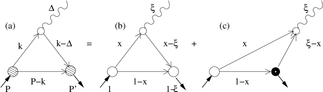
The B-S amplitude and equation is pictured in Fig 1.

Note that the solution requires a set of coupled equations for the vertices, , self mass of the quark (S-D equation), and the B-S amplitude. The Kernal for a perturbative calculation is given by the sum of all irreducible diagrams. For nonperturbative theories like QCD one must use models.
4.1.1 Problems With Instant Form of B-S Equation
About a half century ago an important paper by Wick[19] pointed out a number of serious problems with the B-S equation and B-S amplitude. One of the problems is the dependence on the relative time (or relative energy) variable, whose physical meaning never was clear. He found a solution to this problem via the Wick rotation to Euclidean space. This has wide application, and is still used in hadronic physics. Since this problem has been solved by the light cone formulation we do not review this idea, but aspects will appear later in this review.
4.2 Light Cone Bethe-Salpeter Equation
As discussed above, in order to obtain a B-S wave function for hadronic physics one must also solve the Schwinger-Dyson equation for the dressed quark propagator, which we discuss in the following section. In any case, models are needed for QCD. Here we discuss some early models of the light cone formulation of the B-S equation and applications to the pion form factor.
Since in the infinite momentum frame the pair creation and annihilation processes are suppressed[20], it has many of the attributes of the light cone formulation. In an early paper[21] QED at infinite momentum was treated, and this work has been used recently for obtaining a light cone S-D equation, discussed in the next section. The light cone form of the B-S equation can be obtained by using the -momentum frame[22] or projection onto the light cone[23]. In momentum space, using the notation for the momenta of the two quarks , with , the light cone equation for the B-S wave function, is
In this form one assumes that the mass, m, of the quark is a constant constituent quark mass, and uses a model for the kernel.
4.3 Application of Light Cone B-S Amplitudes to Pion Form Factor
In this subsection we consider applications of the light cone formalism to the pion form factor. The importance of the light cone formalism to study the transition of the pion form factor from a low-momentum region in which nonperturbative effects dominate is first reviewed, followed by treatment with a fixed quark mass, and then the most recent work with a running quark mass. See Sections 8 and 9 for details on l-c wave functions.
4.3.1 Light Cone Wave Function and Transition to Asymptotic QCD
One of the interesting problems in the past two decades is the nature of the transition from the low-momentum region of nonperturbative QCD to the asymptotic region of perturbative QCD. This problem has been studied theoretically for many years, such as the modified quark distribution functions[24], and experimentally. An early application of light cone methods[5, 25] was simply the use of a light cone vs instant form pionic wave functions. The result is quite startling and a dramatic illustration of the advantage of a light cone representation.
Given the wave function of the pion, , for the low-momentum or soft part of the pion form factor with a nonrelativistic wave function the pion form factor is simply
| (51) |
On the other hand it is known that the high momentum transfer (hard) limit perturbation diagrams can be used, with the result[26]
| (52) |
with a similar result obtained by others[27]. It is of great interest to know when perturbation theory can be applied, which is when the nonperturbative soft contributions become smaller than the high-Q contributions. In an attempt to study this a nonrelativistic harmonic oscillator wave function
| (53) |
was used[6]. Even at 10 GeV2 the soft part dominates the hard term. On the other hand, recognizing that even at 1 GeV2 relativistic effects are important, a calculation with the the same wave function in the light front representation[5]:
| (54) |
with N a normalization constant, has been carried out. The results are shown in Fig 2.

As one can see by comparing the light cone (LC) with the instant form (IF) curves, at Q2 greater than about 0.5 GeV2 the relativistic corrections become increasingly important. The curve labeled gives the limit of the hard scattering process[26]. In the light cone model the soft part of the form factor becomes smaller than the asymptotic hard part for , while in the nonrelativistic instant form[6] the soft part dominates until very high Q2. A vastly different interpretation of the transition from soft to hard QCD results.
4.3.2 Light Cone B-S Amplitude for Pion Form Factor
There have been a number of studies of the soft (nonperturbative) pion elastic form factor using light cone or other relativistic models [28, 29] and an early study[30] using light cone wave functions to test the amplitudes of Ref.[24], as well as the work of Ref.[5].
In this subsection we discuss the study of the B-S equation for the pion amplitude[31] with a calculation of the pion form factor including both the soft and hard parts. The starting point is the light cone B-S equation, Eq.(4.2), using the kernel , with the one gluon exchange kernel used to get the hard asymptotic form for the pion form factor[26, 27], and modeled to give the soft confining part:
with b an interaction strength, and m is a mass parameter. The form factor is given by
| (56) |
The B-S amplitude is constrained by 1) normalization, 2) the pion decay constant, , and 3) the pion mass. The pion mass is quite difficult to fit with this model and the best fit to the other parameters resulted in a pion mass of 356 MeV. To obtain a solution, the spinors are first projected out. Expressing the B-S amplitude as , where is the melosh operator[32, 10] and are the quark light cone spinors. After projecting out the spinors, the B-S equation for is solved using the technique of expansion in hyperspherical harmonics[22].
The result for the pion form factor is shown in Fig. 3.

The prediction is that the asymptotic part of the B-S amplitude dominates by 10-15 GeV2. Other light cone model calculations[25] gave similar results.
4.3.3 The Running Quark Mass and the Pion Form Factor
In addition to the transition from soft to hard processes dominating hadronic form factors, as one goes from the nonperturbative to the perturbative regions of momentum transfer the effective quark mass also undergoes an evolution from the constituent mass of low-energy quark models to the current quark mass in the QCD Lagrangian. This can be understood most directly by considering the quark propagator, which has the form
| (57) |
where the running quark mass is given by . The functions are determined by a set of self-consistent equations in the Schwinger Dyson formalism, which we review in the following section. is expected to undergo its transition from the constituent mass of about 300 MeV to a few Mev for u and d quarks at about 1 GeV.
The effect of this running quark mass on the pion form factor was studied some years ago[33], and in greater detail recently[14]. The pion form factor, given by Eq.(56) and the discussion following that equation, is modified if one includes the dressed quark vertex. The elastic pion form factor can be written as
| (58) | |||||
where == and = in the initial pion rest frame, =0. The helicity of the quark(antiquark) is denoted as . The B-S amplitude is the one used in Ref.[31]
| (59) |
where , defined in Eq.(54) is the radial wave function and is the spinor wave function. The Ball-Chiu[34] ansatz is used for the vertex (see the discussion in the next section)
| (60) | |||||
In order to consistently determine the running quark mass, the S-D equation must be solved in a light cone representation, which is reviewed in the next section. In Ref.[14] models were used. For the crossing antisymmetric (CA) parameterization the model is
| (61) |
where = 5 MeV and = 220 MeV are the current and constituent quark masses, respectively. The parameters and are used to adjust the shape of the mass evolution. For the CA picture the two sets of parameters used are = (0.95,0.63) [Set 1] and (0.28,0.55) [Set 2] GeV2. The resulting , with , is shown in Fig. 4.

The results of this model for the pion form factor are shown in Fig. 5.

In comparison with Fig. 3 it is clear that the running quark mass must be taken into consideration in order to trace the evolution from the soft perturbative region to the asymptotic region.
4.3.4 Other Light Cone Calculations of the Pion Form Factor
There has not been much experimental progress in extending accurate measurements of the pion elastic form factor to higher momentum transfers, and there is little hope in that the region above 10 GeV2 will be reached soon. There have been suggestions for improving the perturbative calculations, such as Refs.[35, 36, 37], but detailed calculations of the pion form factor from the soft to the hard regions of momentum transfer require models of the nonperturbative part, and little progress has been made over the past decade. This is unfortunate, since the soft to the hard transition for the pion occurs at a much lower momentum transfer than for the nucleon, but the experiment is quite difficult.
4.4 Low Energy Theorems, Chiral Symmetry, and Light Cone Field Theory
Although light cone field theory is generally most important at high momentum transfers, due to the difficulty in carrying out Lorentz transformations in the instant form (as discussed above), there has been at least one important application at very low energies. We briefly review the soft pion theorems for threshold pion photoproduction and the importance of a light cone formulation. A complete discussion with references can be found in Ref. [38].
The amplitude for pion photoproduction with a nucleon target, has three isospin amplitudes, . A model-independent expansion in the low energy parameter gives[39]
| (62) |
or in the soft pion limit
| (63) |
Standard quark models have a great difficulty with these model-independent predictions. The main problem is that the pion photoproduction processes are related to pion exchange currents, and standard quark models give very different predictions at low energy than hadronic models[40]. As discussed in Ref. [38], the low-energy limit in standard quark models gives
| (64) |
This is a serious violation of low energy theorems, which is also found in chiral quark models[40].
This problem is resolved in light cone field theory models. An interesting observation is that for the calculation of the standard pion exchangs process is replaced by the instantaneous term[27]. It was shown in [38] that with a standard light cone harmonic oscillator model
| (65) |
the low-energy theorem predictions of Eq.(4.4) are satisfied. It should also be noted that the calulation of the amplitude does not agree with low-energy theorems, and that the measurement of the threshold cross section[41] obtained a result for the amplitude also in disagreement with low-energy theorems.
5 Light Cone Representation of the Quark Schwinger-Dyson Equation
In this section we discuss the light cone formulation the quark Schwinger-Dyson Equation (SDE). There has been a great deal of interest in the SDE for hadronic physics, with excellent reviews[42, 43]. The Schwinger-Dyson (S-D) formalism is a technique for obtaining the dressed quark propagator; although this propagator is not in itself physical, it can be used to obtain nonperturbative hadronic strucdture. We review this in the next section. The quark propagator in space-time is defined as the correlator
| (66) |
where T is the time-ordering operator. Since the propagator is diagonal in color, the propagator can be written as , with no sum on the color index a. The S-D formalism starts with an exact expression for the quark propagator and explores models to obtain solutions in the presence of nonperturbative effects.
5.1 Schwinger-Dyson Formalism
The full dressed quark propagator satisfies the Schwinger-Dyson equation (SDE). (See Fig 6):
| (67) |
where and are the dressed quark-gluon vertex and dressed gluon propagator, is a SU(3) operator in color space, is a Dirac operator, with Greek letters representing Lorentz indices and latin letters standing for color indices. The SDE is illustrated in Fig.6
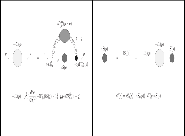

The renormalized vertex is obtained from the vertex SDE
| (68) |
where Z is a renormalization constant and the kernel is related to the dressed gluon propagator . This is illustrated in Fig. 7
The necessary ingredients for obtaining solutions are the dressed vertex and kernel. In practice, the dressed vertex is modeled using symmetries, and the main result of S-D calculations for applications to hadronic physics, in addition to the dressed quark propagator itself, is the dressed Gluon kernel. The transverse part of the dressed vertex is constrained by the Ward-Takahashi identity (see Ref[18] for detailed discussions)
| (69) |
which is an extension to nonvanishing momentum transfer of the Ward identity,
| (70) |
This leads to the Ball-Chiu ansatz, Eq.(60), and the Curtis-Pennington forms[44], discussed in detail in Ref.[42].
The general form of the gluon propagator is
| (71) |
where is the gauge parameter. The Landau gauge corresponds to the choice of , while a so-called Feynman-like gauge corresponds to the choice
| (72) |
for the model gluon propagator.
5.1.1 Constraints on Quark Propagator
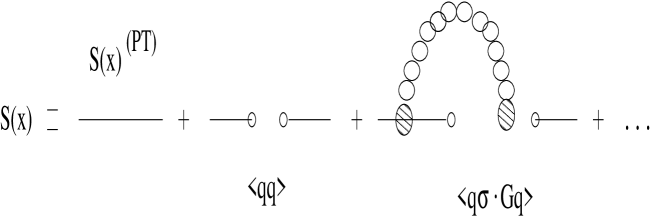
One approach to the treatment of the nonperturative aspects of QCD correlators is to use the operator product expansion, which implies a continuation to large momenta. The operator product expansion of the quark propagator is
| (73) |
where is the quark condensate and is the mixed condensate. This is illustrated in Fig. 8.
The condensates are vacuum expectation values of local operators, and therfore are gauge invariant constants. The quark condensate has been known for many decades, and the mixed constant is somewhat uncertain, but has been estimated using the QCD sum rule method. These condensates can be used to constrain the S-D solutions by the relationships in Euclidean space
| (74) | |||||
with the notation that the Euclidean squared momentum. Another constraint is given by
| (75) |
with M=B/A.
5.1.2 Rainbow Approximation For SDE
The rainbow approximation corresponds to the choice of
| (76) |
This is the main feature of the Global color model[45], reviewed in Ref.[43]. Using the Feynman-like gluon propagator of Eq.(72) the self mass is given as
| (77) |
In this rainbow approximation the quark SDE becomes a set of coupled integral equations
| (78) |
There have been many applications of this model. The vertex for the SDE, Eq.(68) without the perturbative term has the form of a B-S amplitude for a bound quark-antiquark state, i.e., a meson. The B-S equation for a meson as a bound state with momentum P is
| (79) |
where a,b are the color indices of the quark, antiquark, x is the momentum fraction of the quark, and K is the kernel. If one is given solutions to the quark SDE this provides a model of mesonic properties (see, e.g., [46, 47, 48, 49]). As discussed in the previous section, one of the most important studies of hadronic properties is the transition from the soft nonperturbative to the hard perturbative region of momentum transfer, which is best done in a light cone representation. For this reason it would be most valuable to have a light cone S-D solution to use to get hadronic B-S amplitudes, analogous to Eq.(79). We now discuss the first successful light cone solutions of the quark SDE.
5.2 SDE and Quark Propagator in a Light Cone Representation
The method used for solving Eq. (5.1) in a light cone representation in Ref.[13] is to use a technique introduced originally for perturbation theory[50]. Chang and Ma showed how the rules of light cone perturbation theory [LCPT] can be derived in the infinite momentum frame from the usual covariant Feynman rules simply by changing into light cone variables:
An important feature of the new rules is that the range of integration over the variable becomes finite
where is the “plus” (longitudinal) component of the external momentum. This feature is related to the fact that in LCPT there are no diagrams with lines going backwards in time and no vacuum diagrams (with the exception of zero-modes and instantaneous terms in fermion propagators). This is a crucial property of light cone field theory, since it simplifies tremendously the structure of the vacuum.
An important consideration is the form of the integrals needed for the calculation of the quark self-energy in the SDE. We are faced with the non-perturbative self-energy diagram seen in Fig. 6. The integrals occuring in the SDE diagram can be written as a sum of terms of the form:
| (80) |
where the contains factors coming from the quark propagator and possibly from the dressed vertex function, contains factors coming from the gluon propagator and also possibly from the dressed vertex function, and the factors of come from Dirac operators. Since the external momentum is held fixed during this integration, possible factors of and possible dependence of the Green’s functions on are not relevant to the analysis below. Consider first the scalar case, in (80), i.e., no factors . Using the variables:
the integral in (80) becomes:
| (81) |
where all the integrals are over the entire real line, and
.
In Ref.[13] it was shown that if all the singularities of the functions and occur on or below the real axis, only the interval in the integration over contributes to the integral. The model must ensure that the integrals are ultravioletly convergent and thus closing the contour with a semicircle at infinity introduces no additional contribution. The integral in (81) then becomes
| (82) |
It should be noted that to preserve important features of light cone theory (here reflected in the integral over being over a finite range) one must make assumptions about the location of the singularities in and . These assumptions are much like the ones necessary to justify a Wick rotation, however, the method of Ref.[13] allows one to solve the quark SDE for time-like values of the momentum , which is difficult to do after a Wick rotation.
The model gluon propagator is
| (83) |
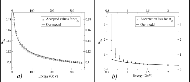
The parameter for a Feynman-like gauge see Eq.(72) and for Landau gauge. It has been shown[51] that renormalization group arguments yield an approximate relation between the renormalized coupling constant, the renormalized gluon propagator and the effective coupling:
| (84) |
where the subscript denotes renormalized quantities, and is the effective running coupling constant. One model used the polynomial form
| (85) |
and the parameters of the model were chosen to fit the PDG[52] values, shown in Fig. 9.
A sample result of the calculation using the iterative procedure is shown in Fig. 10
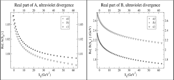
In Fig. 11 the results of a calculation of the light cone SDE are shown, with , the Euclidean momentum squared. The parameters for this calculation gave a reasonably good fit to and , but a rather large value for the mixed condensate. It has a strong infra-red enhancement.
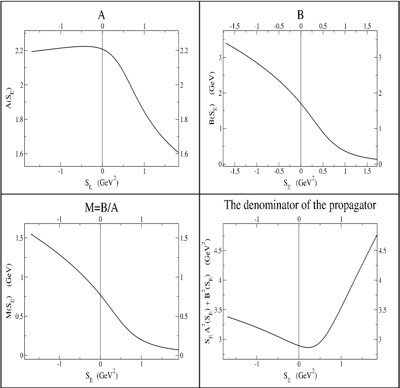
The results for the effective quark mass are too large at low momentum, but the evolution in is reasonable. A most interesting aspect of this calculation is the ability to calculate the quark propagator in the time-like region.
The polynomial model used to obtain the results in Figs. 9, 11 describes an infrared-enhanced gluon propagator. Although this can give confinement, it cannot give the QCD nonperturbative midrange attraction. On the other hand the instanton model can give the strong midrange attraction, even though it does not give the observed confinement. The instanton form of the gauge color field is obtained in a SU(2) Euclidean classical model[53]
| (86) | |||||
where are given in Ref.[54] and for , the instanton size, the instanton liquid model[55] is used. The quark propagator in the instanton/anti-instanton medium, , has been derived in this model[56], giving
| (87) | |||||
where , the instanton density , , and the are modified Bessel functions of the first and second kind, respectively.
In Ref. [13] a number of calculations were done with both the polynomial infra-red enhancement and the instanton contribution, with various choices of the form to check for double-counting. See that references for the results and details on how the calculation is done.
This approach is most promising when coupled with the methods for using SDE solutions to get mesonic properties as in Refs. [46, 47, 48, 49]. In the previous work, in which the key idea given by Eq.(79) is used, the use of instant form SDE solutions limits the work to low momentum transfer, while with the light cone solutions described in this section all momentum transfer can be studied. This is an exciting prospect for future research in light cone physics.
6 Deeply Virtual Compton Scattering and Skewed Parton Distributions
In recent years there has been a great interest in deeply virtual compton scattering (DVCS) arising from the use of this reaction for studying generalized parton distributions[57, 58], also called off-forward or skewed parton distributions (SPDs). See Ref.[59] for a recent review with references. Virtual Compton scattering from a hadron, i.e., the e + e’ reaction on the hadron, is the reaction
| (88) |
where q (q’) are the momenta of the incoing virtual (outgoing real) photons and P (P’=P-) are the momenta of the initial (final) hadron, H. The DVCS amplitude is
| (89) |
with T the time-ordered product of the electromagnetic currents.
DVCS is the high limit of VCS, and has some of the physical as well as mathematical aspects of deep inelastic scalleting (DIS). A striking aspect of inelastic scattering with a hadronic target H
| (90) |
is that the differential cross section factorizes
| (91) |
where is the leptonic tensor
| (92) |
with the (incoming, outgoing) electron four-momenta, and is the hadronic tensor. For DIS the “handbag” diagram shown in Fig. 12

dominates. In the diagram is the hadron target and the sum is taken over intermediate states , expressing the hadronic tensor as
| (93) |
in terms of the matrix element of the current commutator n the hadronic state with spin index . For more than two decades DIS has been used to learn about parton distributions. (See, e.g., Ref[64])
For DVCS the amplitude (not the cross section as in DIS) is dominated by the handbag diagrams, shown in Fig. 13.

In the diagram the target is shown as , the B-S amplitude of the hadron, which gives the vertex of H, a quark, and the residual system. After a review of the kinematics we give a brief review of DVCS on a nucleon and review recent developements on skewed parton distributions of the pion, where newly developed B-S amplitudes can be used to compare with experiment.
6.1 Kinematics for DVCS. Skewness
With the notation for a light cone four vector , choosing the frame with , and defining the four momentum transfer , the kinematics of VCS with a hadron target of mass is
| (94) |
| (95) |
with
| (96) |
the skewedness parameter describing the asymmetry in plus momentum. The squared momentum transfer is
| (97) |
In a frame where the incident spacelike photon has
| (98) |
In deeply virtual Compton scattering (DVCS) where is large compared to the mass and , one obtains
| (99) |
i.e. plays the role of the Bjorken variable in DVCS. For a fixed value of , the allowed range of is given by
| (100) |
6.2 DVCS on the Nucleon
There has been a great deal of interest in elastic and inelastic form factors of the nucleon for many years for tests of quark models and quark distributions. The interest in DVCS was the realization that new information on quark structure of the nucleon can be obtained, and it can be directly related to the elastic structure functions. First recall the elastic form factors of the nucleon, ,
| (101) |
with the nucleon spinor, the axial form factors
| (102) |
where is the axial vector current, and the pseudoscalar form factor
| (103) |
The VCS amplitude with the handbag diagrams, Fig. 13, have the form
| (104) |
where is the quark propagator and
| (105) |
When the DVCS amplitude is expressed in light cone variables, the quark matrix element is expressed in terms of skewed quark distributions which in the notation of Ref.[57] are to twist two
| (106) | |||||
These skewed distributions satisfy the sum rules
| (107) | |||||
In recent years there have been studies of higher twist effects for DVCS. For a recent review of DVCS with a nucleon target and references to recent work see Ref. [65], and a light cone wave function representation of DVCS is discussed in Ref. [62]. There is a great interest in new experiments to measure skewed quark distributions. These were discussed at the international workshop Light cone 2002[4].
We now turn to DVCS and skewed quark distribution on the pion.
6.3 DVCS on the Pion
The skewed quark distributions of the pion,, are defined by the integral
| (108) |
where in a light front representation. Note that the path-ordered exponential of the gauge field, , required by gauge invariance[58] in Eq. (108) does not appear in the light front gauge . Recalling the definition of the pion form factor, ,
| (109) |
as one can see from Eqs. (109) and (108), the involves one less integration than the form factor due to nonlocality of the current matrix element. The SQDs display characteristics of the ordinary(forward) quark distribution in the limit of and , on the other hand, the first moment of the SQDs is related to the form factor by the following sum rules [57, 58]:
| (110) |
where and we assume isospin symmetry() so that . Note that Eq. (110) is independent of , which provides important constraints on any model calculation of the SQDs.
The diagrams for the SQDs are shown in Fig. 14. In the range of x, , for the BS amplitude is the standard one that determines the pion form fator, as shown in Fig. 14(b), while for an analytic continuation, called the nonvalence BS amplitude is needed, as shown in Fig. 14(c).
The B-S amplitudes (see Sec. 4) needed for the calculation of the SQDs are solutions to
| (111) |
where is the B-S kernel, ,, and is the B-S amplitude. Defining the solution to Eq.(111) when , which is the familiar B-S amplitude, as the valence amplitude, the valence and nonvalence B-S solutions are
| (112) |
In the light front quark model[63] the B-S amplitudes in the two regions are related by
| (114) |
The contribution from the process shown in Fig.14(b) is given by the B-S amplitude, with the valence part of given by
| (115) | |||||
with the internal momenta of the (struck) quark for the final state given by
| (116) |
The contribution from the nonvalence part of , the process shown in Fig.14(c), is given by the B-S amplitude, with the form
| (117) | |||||
with a function of kinematic variables given in Ref[16], is the quark-gauge boson vertex shown as the small white blob in the upper vertices of Fig 14, and and
The contribution from this nonvalence region is obtained by making approximate use of the constraint
| (118) |
so the B-S amplitude is not used. The valence B-S amplitude is modeled by a light cone harmonic oscillator:
| (119) |
Substituting Eq.(119) in Eq.(115) one obtains the valence contribution to the SQDs.
For the pion form factor is given by the valence process. In Fig.15 the valence contribution to is shown. For values of the nonvalence contribution is seen to become significant.

In Figs. 16 and 17, are shown the SQDs, , of the pion for fixed momentum transfer GeV2 () and GeV2 () but with different skewedness parameters , respectively. The solid and cross (x) lines in the nonvalence contributions are the exact solutions obtained from using the B-S equation to obtain for the model of Eq.(119), and an approximation based on Eq.(118). The SQDs at as shown in Figs. 16(a) and 17(a) correspond to the ordinary quark distributions with vanishing nonvalence contributions. The frame-independence of the model calculation is ensured by the area under the solid lines(valence nonvalence) being equal to the pion form factor at given . As one can see from Figs. 16(b-c) and 17(b-c), while the nonvalence contributions are small for small , they are large for large skewdness parameter . It is interesting to note that the instantaneous contribuitons (dotted lines in each figure) become more pronounced as for each . While the instantaneous part of the nonvalence contribution vanishes as as shown in Figs. 16 and 17, the net result of including the on-mass shell propagating part does not vanish as and consequently causes a discontinuity to the zero value of . However, such discontinuity at is just an artifact due to the difference in the behavior between the gauge boson vertex ( in Ref.[16]) and the hadronic vertex ( in Eq. (115) of our approximate model calculation. See the following subsection for a discussion of and the continuity problem. We have indeed confirmed that the discontinuity at does not occur in the limit of a point hadron vertex as observed in the QED calculation [62]. Thus, for a full analysis of DVCS satisfying factorization theorems, it would be necessary to solve the bound-state B-S equation similar to Eq. (111) for the gauge boson () as well as for the hadron ().
The main approximation in this calculation is the treatment of relevant operator in Eq. (114) connecting the one-body to three-body sector by taking a constant for the quantity , which in general depends on and . The reliability of this approximation was checked by examining the frame-independence of the numerical results and using the sum rule given by Eq. (118). This method seems useful for the present study of the relation between SQDs and the form factor in the nonperturbative regions.


6.3.1 Continuity of Pion DVCS Generalized Parton Distributions
The problem with continuity, discussed in the previous section, is the treatment of the gauge boson vertex, in the nonvalence region, ; i.e., the white blob in Fig.14(c). In Ref[16] the form used was
| (120) |
with and . In [17] an effective light cone wave function was used for the gauge boson wave function:
| (121) |
This model solves the problem of continuity, as shown in Fig. 18


7 Rare Decays
There is currently a great interest in the study of B decays for study of the CKM mixing matrix as a test of electroweak models. The exclusive decay, a rare decay in that it is forbidden for tree-level processes, is particularly interesting, but the theoretical calculation requires hadronic form factors involving nonperturbative physics. There have been many theoretical studies in recent years[66, 67, 68, 69, 70, 71, 72, 73, 74, 75, 76]. Since this decay of B-mesons involves a large energy transfer, it is a natural for a light cone treatment, which has many advantages compared to instant form relativistic quark model treatments[66, 67, 68, 69].
The effective Hamiltonian for the decay process in obtained after integrating out the heavy top quark and the bosons [77]:
| (122) |
where is the Fermi constant, are the CKM matrix elements and are the Wilson coefficients. The important operators to the rare decay are
| (123) |
where is the chiral projection operator and is the electromagnetic interaction field strength tensor. The Wilson coefficients determined by the renormalization group equations(RGE) from the perturbative value are given in the literature (see, for example [78, 79]). After integrating out the terms involving -loops and neglecting the strange-quark mass, the resulting effective Hamiltonian corresponding to Eq. (122) is
where the effective Wilson coefficient (=) is given in Refs [78, 79, 80, 81, 82, 83], and has the form
| (125) | |||||
where the functions is the one-loop matrix element of , describes the long distance contributions due to the charmonium vector resonances via , and represents the one-gluon correction to the matrix element of .
The long-distance contribution to decay is contained in the meson matrix elements of the bilinear quark currents appearing in . The matrix elements of the hadronic currents for transition can be parametrized in terms of hadronic form factors as follows:
| (126) | |||||
and
| (127) | |||||
where and is the four-momentum transfer to the lepton pair and .
The transition amplitude for the decay can be written as
| (128) | |||||
where is the fine structure constant. The differential decay rate for with nonzero lepton mass() is given by
| (129) | |||||
where
| (130) |
with , , , and
| (131) |
Note (Eqs.(129,7)) that only and are necessary for the massless() rare exclusive semileptonic , with not contributing.
The differential branching ratio, is obtained from
| (132) |
with the total width. Another interesting observable, the longitudinal lepton polarization asymmetry(LPA) is defined as
| (133) |
where denotes right (left) handed in the final state. From Eq. (129), one obtains for
| (134) |
The calculation of is similar to the calculation of described in the previous section. An important difference is that in calculatin and the initial and final B-S amplitudes are different, so that in contrast to Eqs.(115) and (117) with in the initial and final state, one needs a and for the initial b-meson final s-meson.
First, if one works in frame, with the weak form factors needed are of the form
| (135) |
and
| (136) |
with the known kinematic functions and given in Ref[15]. The model light front Gaussian wave functions used are
| (137) |
normalized by where and is defined as
| (138) |
The calculations in Ref[15] are done in the purely longitudinal frame with and , and thus the momentum transfer square is timelike. For the valence process, corresponding to Fig 14(b), the calculation is carried out using the model l-f wave functions . For the nonvalence process, corresponding to Fig 14(c), the final state B-S amplitude must be replaced by the function
| (139) |
where is a known function of the kinematic variables. As discussed in the treatment of skewed quark distributions in the previous section, in Ref [15] is taken as a constant, and the reliablity of this approximation is checked by examining the frame-independence of the numerical results.


The results with this model for the differential branching ratios, with and =1.777 GeV, for are shown in Fig. 19(a) and for in Fig. 19(b), respectively. The thick(thin) solid line represents the result with(without) the LD contribution() to given by Eq. (125). One can see that the pole contributions clearly overwhelm the branching ratio near and peaks, however, suitable invariant mass cuts can separate the LD contribution from SD one away from these peaks. This divides the spectrum into two distinct regions [84, 85]: (i) low-dilepton mass, , and (ii) high-dilepton mass, , where is to be matched to an experimental cut. The numerical results for the non-resonant branching ratios(assuming ) are for () and for , respectively. While the data by CLEO Collaboration [86] reported the branching ratio , the data by Belle Collaboration(K. Abe et al.) [86] reported and , respectively. The comparison of the results of this model with other models is given in detail in Ref [15]
The longitudinal lepton polarization asymmetry(LPA) in this model for and as a function of , respectively, in Figs. 20(a) and (b). The results with the LD contributions are shown be the thick solid line, and without by the thin solid line. Further discussion of these results and comparison with other calculations is found in Ref [15].
In conclusion, the rare exclusive semileptonic ( and ) decays are found to be useful for studies of nonperturbative form factors, and the light cone approach is most valuable for the theoretical models.
8 Meson Light Cone Wave Functions
The structure of mesons is of great interest for the study of QCD. With a simple two-body configuration being the lowest Fock state, for certain reactions the pion can be a relatively simple system for theoretical investigations. As discussed in Sec. 4, for high momentum transfer processes the PQCD treatment is adequate. At low and medium momentum transfers nonperturbative effects dominate. In the present section the QCD sum rule method for determining the wave function of the and mesons is reviewed. The pion wave function is of particular interest as there are now experimental studies of the light cone wave function, which is discussed in this section.
In Sec.4 the Bethe-Salpeter amplitude for a two-body bound state, in instant form coordinate space, was discussed, with the light cone B-S amplitude, , given as the solution to the l-c B-S equation, Eq.( 4.2). In order to obtain the correct physical B-S amplitude, also called the light cone wave function, one needs a kernel which gives a satisfactory representation of the field theory being considered. In the applications discussed in previous sections models were used. In the next subsection we discuss the use of QCD sum rules to estimate the pion and rho meson wave functions. Theoretical and experimental work on the direct measurement of the component of the pion wave function is discussed in the following subsection.
8.1 QCD Sum rules for the Pion and Rho Meson Wave Function
We first discuss the pion wave function is some detail, and then give the results for the rho. The light cone wave function of a meson can be obtained from the gauge-invariant matrix element
| (140) |
where (u,d) are the up and down quark fields and is the QCD gluonic color field. We shall work in the fixed point gauge, with the gauge condition , so that the operator . The method of QCD sum rules[87] utilizes an operator product expansion, which leads in a natural way to a twist expansion of the wave function. We briefly review QCD sum rule procedure
8.1.1 Brief Review of the QCD Sum Rule Method
The method of QCD sum rules makes use of a correlator defined in terms of a composite field operators
| (141) |
For mesons the can be taken in the form
| (142) |
with chosen so that the operator creates states with the quantum numbers of the meson under consideration. E.g., for a scalar, pseudoscalar or vector meson or , respectively, are possible choices.
If the correlator satisfies an unsubtracted dispersion relation (in Euclidean space), then can be expressed as
| (143) | |||||
where M is the mass of the stable meson, is a constant, and is the parameter for the beginning of the continuum contribution to the dispersion relation. The QCD sum rule is obtaind by equating the Borel transformation, , of the phenomenological correlator, Eq.(143), to the QCD evaluation of ,
| (144) | |||||
with called the Borel mass. The Borel transformation reduces the importance of the continuum contribution, and results in a rapidly diminishing size of the QCD diagrams with increasing dimension. The QCD side of Eq.144 is of the form
| (145) |
where the are constants obtained by evaluating the QCD diagrams and the are vacuum condensates of dimension . In order of increasing dimension the most important three condensates are
| (146) |
The quark condensate is rather accurately known, with 0.55 GeV3. A typical value for the gluon condensate is .47 GeV4, and for the mixed condensate , with 0.8 GeV2.
8.1.2 QCD Sum Rules For the Light Cone Wave Function
A QCD sum rule analysis of to extract an expansion of the pion l-c wave function with nonperturbative QCD effects was carried out in Ref. [24]. See Refs. [88, 89] for reviews. A study of the l-c wave function vs. light front quark models has also been done using QCD sum rule techniques[90]
Using the fixed point gauge and expanding u(z) about the origin,
one obtains for
(Eq.(140))
| (147) | |||||
. with and proportional to the l-c wave function.
This expression is evaluated using a version of QCD sum rules. Using for the pion composite field operator, the nth term in Eq.(147) is given by the vacuum matrix elements
| (148) |
By evaluating the diagrams up to dimension 6, illustrated in Fig. 21, Chernyak and Zhitnitsky derived the expansion

for the Borel transform of ,
| (149) |
The light cone wave function is obtained from of Eq.(147) by letting and . The light cone wave function is then obtianed from in the gauge with :
| (150) |
The CZ wave function[24], with the normalization , with the pion decay constant 133 MeV, was obtained using the values of the condensates given above. Within the errors in the method an approximate form for the CZ result often used is
| (151) |
with units of This can be compared to the asymptotic light cone wave function[27], also with units of
| (152) |
8.1.3 QCD Sum Rules For The Light Cone Wave Function of the
Treatment of the rho meson, with the composite field operator is quite different for the longitudinal () and the transverse ( currents, for and , respectively.
For the QCD sum rule treatment of Ref [24] is the same as for the , with the quantities given by the expression in Eq.(148) with the operators removed. The resulting expansion of the l-c wave function, using the analog of the diagrams in Fig. 21, in units of 3fρ is approximately
| (153) |
For the quantities corresponding to the given by the expression in Eq.(148) for the are obtained by replacing by in Eq.(148) (with a sum over , of course). The result of the analysis[24] for the transverse rho l-c wave function, in units of 3fρ is approximately
| (154) |
In Fig. 22 the CZ pion l-c pion wave function is compared to the asymptotic l-c pion wavefunction, in units of , for the pion and the transverse rho l-c CZ wavefunction

9 Factorization and Experimental Study of Light Cone Wave Functions
An essential aspect of testing hadronic and nuclear structure by high energy reactions is that amplitudes for such reactions factorize. Consider Fig. 23 with a schematic high energy reaction on a target with
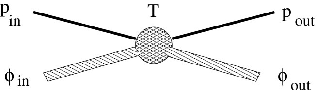
wave function leading to a final state with wave function . The factorization theorem states that the reaction amplitude satisfies the schematic relationship
| (155) |
with the initial and final target wave functions, and represents the parton hard scattering. Factorization is important for the extraction of information for many reactions. For a discussion with references see, e.g., Ref. [89]. The coherent production of dijets with a high energy pion projectile, which we discuss next, is of particular interest because of a recent experimental measurement.
9.0.1 Coherent Diffractive Pion Production of Dijets
The concept of diffractive dissociation is very old in nuclear/particle physics[92], and was extended to QCD in Ref. [93]. The essential idea for pion production of dijets is that for a pion projectile on a nuclear target at high energy, the short-range color zero configuration will traverse the nucleus with little interaction, while the other components will be absorbed. Therefore the component is filtered out and leaves the nucleus to form two jets.
The ) amplitude[94], for high energies with the forward scattering amplitude , where is the total cross section as a function of impact parameter , with this coherent diffractive dissociation production scenerio is
| (156) |
where is the impact parameter, is the total forward cross section of the valence diquark system, and the scattering of the final jets has been neglected, so that their wave function is a plane wave with the relative transverse momentum variable . This is a special case of the factoriation theorem, Eq.(155). Recently, there has been a theoretical study of photoproduction of high energy dijets with nuclear targets[95] which within the approximations leading to Eq.(156) is the reaction
| (157) |
so that the pion valence wave function can also be studied with this reaction.
9.0.2 Experimental Study of the Pion Light Cone Component
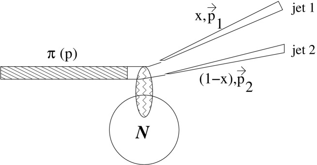
A direct measurement of the light cone meson wave function can be carried out through a high-energy coherent diffractive dissociation of the meson. This was recently done at Fermilab experiment E791[91]. The experiment used a 500 GeV beam with a platinum target.

The diffractive dijets were identified as having their yield depend on , the transverse momentum transfered to the nucleus, by
| (158) |
where is the effective impact parameter squared. The x value of the jet (see Fig. 24) is obtained from
| (159) |
The results of the experiment are shown in Fig. 25. The fit to the data, the solid line in Fig 25 is made with a squared wave function that is a linear combination of the CZ and AS wave functions
| (160) |
Using the relationship for the virtuality of the dijets
| (161) |
for 1.5 GeV 10 GeV2, and the gives a good fit to the data, while in the lower bin the CZ component makes a sizable contribution.
10 Conclusions
The methods of light cone field theory and light front quantum mechanics play a vital role in the extraction of information on the structure of hadrons and nuclei. It has been applied in recent years to hadronic form factors and a variety of reactions, with a great deal of work on the transition from nonperturbative to perturbative QCD treatments of hadronic form factors and deeply virtual reactions with photon projectiles. The use of light cone wave functions is important for extracting information from the decay of heavy-quark hadrons. Quite recently coherent diffractive dissociation and related reactions have begun to provide direct measurements of light cone wave functions. This is an exciting field for theory and experiment, and will continue to provide important informationabout the nature of Quantum Chromodynamics.
ACKNOWLEDGEMENTS The author would like to acknowledge many helpful discussions with Matthias Burkhardt, Mikkel Johnson, and Stephan Pate, coorganizers of the Light cone 2002 International Workshop, as well as many of those attending the workshop. This work was supported in part by the NSF grant PHY-00070888 and in part by the DOE contract W-7405-ENG-36.
References
- [1] P.A.M. Dirac, Rev. Mod.Phys. 21, 392 (1949).
- [2] S.J. Brodsky, H.-C. Pauli and S.S. Pinsky, Phys. Reports 301, 299 (1998).
- [3] J.R. Hiller, S.S. Pinsky and U. Trittmann, Phys. Rev. D66, 125015 (2002).
- [4] Light Cone 2002: Structure of Hadrons and Nuclei on the Light Cone, LANL, August, 2002.
- [5] O.C. Jacob and L.S. Kisslinger, Phys. Rev. Lett 56, 225 (1986).
- [6] N. Isgur and C.H. Llewellyn Smith, Phys. Rev. Lett 52, 1080 (1984).
- [7] L.L. Foldy, Phys. Rev. 122, 275 (1961).
- [8] H. Leutwyler and J. Stern, Ann. phys. 112, 94 (1978).
- [9] B.L.G. Bakker, L.A. Kondratyuk and M.V. Terentev, Nucl. Phys. B158, 497 (1984).
- [10] L.A. Kondratyuk and M.V. Terentev, Sov. J. Nucl. Phys. 31, 561 (1980).
- [11] B. Bakamjian and L.H. Thomas, Phys. Rev. 92, 1300 (1953).
- [12] B.D. Keister and W.N. Polyzou, Adv. Nucl. Phys. 20 (1991), p.226
- [13] L.S. Kisslinger and O. Linsuain, Phys. Rev. C66, 045206 (2002).
- [14] L.S. Kisslinger, H-M. Choi and C-R. Ji, Phys. Rev. D63, 113005 (2001); H-M. Choi, L.S. Kisslinger and C-R. Ji, Nuc. PhysProc. Suppl. 108, 310 (2002)
- [15] H-M. Choi, C-R. Ji and L.S. Kisslinger, Phys. Rev. D65, 074032 (2002).
- [16] H-M. Choi, C-R. Ji and L.S. Kisslinger, Phys. Rev. D64, 093006 (2001).
- [17] H-M. Choi, C-R. Ji and L.S. Kisslinger, Phys. Rev. D66, 053011 (2001).
- [18] C. Itzykson and J.B. Zuber, “Quantum Field Theory” (McGraw-Hill, New York, 1986).
- [19] G.C. Wick, Phys. Rev. 96, 1124 (1954).
- [20] S. Weinberg, Phys. Rev. 150, 1313 (1966).
- [21] S-J. Chang and S-K Ma, Phys. Rev. 180, 1506 (1969).
- [22] M. Sawicki, Phys. Rev. D32, 2666 (1985).
- [23] S.J. Brodsky, C-R Ji and M.Sawicki, Phys. Rev. 32, 1530 (1985).
- [24] V.L. Chernyak and A.R. Zhitnitsky, Nucl. Phys. B201, 492 (1982); B214, 547(E) (1983).
- [25] L.S. Kisslinger and S.W. Wang, Nucl. Phys. B399, 63 (1993).
- [26] G.R. Farrar and D.R. Jackson, Phys. Rev. Lett. 43, 246 (1979).
- [27] G.P. Lepage and S.J. Brodsky, Phys. Rev. D22, 2157 (1980).
- [28] Z. Dziembowsky, Phys. Rev. D37, 778 (1988).
- [29] F.Cardarelli et. al., Rev. D53, 6682 (1996).
- [30] Z. Dziembowsky and L. Mankiewicz, Phys. Rev. Lett. 58, 2175 (1987).
- [31] O.C. Jacob and L.S. Kisslinger, Phys. Lett. B243, 323 (1990).
- [32] H.J. Melosh, Phys. Rev. D9, 1095 (1974).
- [33] L.S. Kisslinger and S.W. Wang, hep-ph/9403261 (1994).
- [34] J.S. Ball and T.-W. Chiu,Phys. Rev. D22, 2542 (1980).
- [35] S.J. Brodsky, C-R. Ji, A. Pang and D.G. Robertson, Phys. Rev. D57, 245 (1998).
- [36] A. Szczepaniak, C-R. Ji and A. Radyushkin, Phys. Rev. D57, 2813 (1998).
- [37] S.W. Wang and L.S. Kisslinger, Phys. Rev. D54, 5890 (1996).
- [38] Z-J. Cao and L.S. Kisslinger, Phys. Rev. Lett. 64, 1007 (1990).
- [39] N. Kroll and M. Ruderman, Phys. Rev. 93, 233 (1954).
- [40] M. Beyer, D. Drechsel and .M. Giannini, Phys. Lett. B122, 1 (1983); S. Scherer, D. Drechsel and L. Taitor, Phys. Lett. B193, 1 (1987); D. Drechsel and L. Taitor, Phys. Lett. B148, 413 (1984).
- [41] R. Beck et. al., Phys. Rev. Lett. 65, 1841 (1990).
- [42] C. Roberts and A.G. Williams, Prog. Part. Nucl. Phys. 33 447 (1994).
- [43] P.C. Tandy, Prog. Part. Nucl. Phys 39, 117 (1997).
- [44] D.C. Curtis and M.R. Pennington, Phys. Rev. D42, 4165 (1990).]
- [45] R.T. Cahill and C.D. Roberts, Phys. Rev. D32, 2419 (1985).
- [46] P. Maris and C.D. Roberts, Phys. Rev. C56, 3369 (1997).
- [47] M. Burkardt, M.R. Frank and K.L. Mitchell, Phys. Rev. Lett. 78, 3059 (1997).
- [48] P. Maris and P.C. Tandy, Phys. Rev. C60, 055214 (1999).
- [49] P. Maris and P.C. Tandy, Nucl. Phys. A663, 401 (2000).
- [50] S. Chang and S. Ma, Phys. Rev. 180, 1506 (1969).
- [51] U. Bar-Gadda Nucl. Phys. B163, 312 (1980).
- [52] Particle Data Group, Review of Particle Physics, The European Physical Journal C15, 1 (2000).
- [53] A.A. Belavin, A.M. Polyakov, A.S. Schwartz and Yu.S. Tyupkin, Phys. Lett. B59, 85 (1975).
- [54] G. ’t Hooft, Phys. Rev. D14, 3432 (1976).
- [55] T. Schffer and E.V. Shuryak, Rev. Mod. Phys. 70, 323 (1998)
- [56] P.V.Pobylitsa, Phys. Lett B226, 387 (1989)
- [57] X. Ji, Phys. Rev. Lett 78, 610 (1997); Phys. Rev.D55, 7114 (1997).
- [58] A.V. Radyushkin, Phys. Rev. D56, 5524 (1997).
- [59] M. Diehl, Phys. Rept. 388, 41 (2003).
- [60] R. A. Amendolia et al., Phys. Lett. B178, 435 (1985).
- [61] J. Volmer et al., Phys. Rev. Lett. 86, 1713 (2001)
- [62] S.J. Brodsky, M. Diehl and D.S. Hwang, Nucl. Phys. B596, 99 (2001).
- [63] C.-R. Ji and H.-M. Choi, Phys. Lett. B513, 330 (2001).
- [64] F.E. Close, “An Introduction to Quarks and Partons”, Academic Press (New York, 1979).
- [65] A.V. Belitsky, D. Mller and A. Kirchner, Nucl. Phys. A629, 323 (2002).
- [66] W. Jaus and D. Wyler, Phys. Rev. D41, 3405 (1990); C. Greub, A. Ioannissian and D. Wyler, Phys. Lett. B346, 149 (1995).
- [67] C. Q. Geng and C. P. Kao, Phys. Rev. D54, 5636 (1996).
- [68] D. Melikhov, N. Nikitin, and S. Simula, Phys. Lett. B410, 290 (1997); 430, 332 (1998).
- [69] D. Melikhov and N. Nikitin, Phys. Rev. D57, 6814 (1998).
- [70] W. Roberts, Phys. Rev. D54, 863 (1996); G. Burdman, Phys. Rev. D52, 6400 (1995).
- [71] P. Colangelo et al., Phys. Rev. D53, 3672 (1996); Phys. Lett. B395, 339 (1997).
- [72] P. Ball, hep-ph/9802394, JHEP 9809, 005 (1998).
- [73] P. Ball and V. M. Braun, Phys. Rev. D58, 094016 (1998).
- [74] T. M. Aliev et al., Phys. Lett. B400, 194 (1997).
- [75] R. Casalbuoni et al., Phys. Rep. 281, 145 (1997).
- [76] D. Du, C. Liu, and D. Zhang, Phys. Lett. B317, 179 (1993).
- [77] B. Grinstein, M.B. Wise, and M.J. Savage,Nucl. Phys. B319, 271 (1989).
- [78] A. J. Buras and M. Mnz, Phys. Rev D52, 186 (1995).
- [79] M. Misiak, Nuc. Phys.B393, 23 (1993); . 439, 461(E) (1995).
- [80] A. Ali, T. Mannel and T. Morozumi, Phys. Lett. B273, 505 (1991); A. Ali, Acta Phys. Pol. B 27, 3529 (1996).
- [81] C. S. Kim, T. Morozumi, and A. I. Sanda, Phys. Rev. D56, 7240 (1997).
- [82] T. M. Aliev, C. S. Kim, and M. Savci, Phys. Lett. B441, 410 (1998).
- [83] Z. Ligeti and M. B. Wise, Phys. Rev. D53, 4937 (1996).
- [84] J. L. Hewett, Phys. Rev. D53, 4964 1996; F. Krger and L. M. Sehgal, Phys. Lett. B380, 199 (1996)..
- [85] A. Ali, G. F. Guidice, and T. Mannel, Z. Phys. C 67, 417 (1995).
- [86] S. Anderson et al., CLEO Collaboration, hep-ex/0106060, Phys. Rev. Lett 87, 181803 (2001). K. Abe et al., Belle Collaboration, hep-ex/0107072, 2001 Lepton Photon Conference. A. Abashian et al., Belle Collaboration, hep-ex/0102018, Phys. Rev. Lett 86, 2509 (2001). B. Aubert et al., BaBar Collaboration, hep-ex/0102030, Phys. Rev. Lett 86, 2515 (2001).
- [87] M. A. Shifman, A. I. Vainshtein, and V. I. Zakharov, Nucl. Phys.B147 (1979) 385; 448.
- [88] V.L. Chernyak and A.R. Zhitnitsky, Phys. Rep 112, 173 (1984).
- [89] G. Sterman and P. Stoler, Ann. Rev. Nucl. Part. Sci 43, 193 (1997)
- [90] V.M. Belyaev and M.B. Johnson, Phys. Lett.B423, 379 (1998).
- [91] Fermilab E791 Collaboration, E.M. Aitala et. al., Phys. Rev86, 4768 (2001); .; D. Ashery, Comments Mod. Phys. 2, A235 (2002).
- [92] E.L. Feinberg and I.Ia. Pomeranchuk, Nuovo Cim, Suppl. III, 652 (1956).
- [93] G. Bertsch, S.J. Brodsky, A.S. Goldhaber and J.G. Gunion, Phys.Rev. Lett. 47, 297 (1981).
- [94] L. Frankfurt, G.A. Miller and M. Strikman, Phys. Lett. B304, 1 (1993); Found Phys. 30, 533 (2000).
- [95] V.M. Braun et al, Phys. Rev. Lett. 89, 172001 (2002).