Chapter 1 Introduction

CP symmetry violation was discovered several decades ago in neutral kaon decays [1]. Effects of CP symmetry breaking have been also recently observed in $B$ meson decays [2, 3], but kaon physic continues being an exceptional ground to study this kind of phenomena. The analysis of the parameters that describe CP violation constitutes a great source of information about flavour changing processes and, in the Standard Model, they can provide us with information about the worst known part of the Lagrangian, the scalar sector, where CP violation has its origin.

The main CP-violating parameter in the kaon decays is $\varepsilon_{K}^{\prime}/\varepsilon_{K}$, for which there exist very precise experimental measures $\mbox{Re }(\varepsilon_{K}^{\prime}/\varepsilon_{K})=(1.66\pm 0.16)\times 10^{-3}$ -see Chapter 2 for definitions and discussions. Experimental data for this quantity and another CP–violating parameters –as well as other quantities related with different fundamental aspects in particle physics as flavour changing neutral currents or quark masses– are based on the analysis of observables involving hadrons, that interact through strong interactions. In particular, these observables are governed in a decisive way by the non-perturbative regime of Quantum Chromodynamics (QCD), the theory describing strong interactions. At low energies –in the non-perturbative regime– QCD is not completely understood, so it is not easy to get theoretical predictions for the hadronic matrix elements involved in these processes without large uncertainties. Any improvement in the calculation of these hadronic matrix elements would thus been fundamental in the understanding of experimental CP-violating results. The goal is twofold, on one hand we pretend to analyze theoretically with great precision some observables in the Standard Model, specially those related to the CP-violating sector which is embedded in the scalar sector, the worst known part of the Standard Model lagrangian. On the other hand, the precise knowledge of the Standard Model predictions for CP-violating observables can serve to unveil the existence of new physics and check the validity of certain models beyond the Standard Model.

The main problem is dealing with strong interactions at intermediate energies. At very low and high energies we can use Chiral Perturbation Theory (CHPT) [4, 5] and perturbative QCD respectively, that are well established theories. They let us do reliable calculations using next orders in the expansion as an estimate of the error associated to them. Several methods and approximations have been developed in order to try to suitably describe the intermediate region. Any reliable calculation give a good matching between the long- and short- distance regions. The most important of these methods are listed in Chapter 5 and their predictions for several CP-violating parameters are commented along the different chapters of this Thesis.

The basic objects that are needed for the description of the low energy physics are the two-quark currents and densities Green’s functions. The couplings of the strong CHPT lagrangian are coefficients of the Taylor expansion in powers of masses and external momenta of some of these Green’s functions. While other order parameters needed in kaon physics such as $B_{K}$, $G_{8}$, $\mbox{Im }G_{E}$ or $G_{27}$ are obtained by also doing the appropriate identification of the coefficients in the Taylor expansion of integrals of this kind of Green’s functions over all the range of energies. See Section 2.4.1 of Chapter 2 for more details. A good description of Green’s functions would thus provide predictions for the parameters we are interested in. A description of a general method to perform a program of this kind is given in Chapter 5 and some possible applications of it are discussed in the conclusions.

This Thesis is organized in two parts. In the first part, Chapters 1-3, we describe the framework in which the Thesis has been developed and establish the definitions and notation necessary in the second part.

In the next section of this chapter we give an overview of the Standard Model, explaining the different sectors in which it can divided and the grade of knowledge we have about each of them. We define the symmetry CP and discuss in which conditions it can be measured experimentally. Discussions about the value of the SM parameters $m_{s}$ and $|V_{us}|$ calculated in [6, 7] are also provided in this chapter. The Chapter 2 is a more detailed description of the theory involved in the CP violation in $K$ decays, in which we define the main CP-violating observables and outline the theoretical calculation of these parameters. The present experimental and theoretical status of direct CP violation in the kaon decays is also given. In Chapter 3 we introduce CHPT, collect the Lagrangians at leading and next-to-leading order in this theory and discuss the values of the couplings of these Lagrangians. In addition, leading order in the chiral expansion predictions for some CP-violating observables are given.

The second part of the Thesis, Chapters 4-7, is composed by the calculations of some of the CP-violating observables defined before. In Chapter 4 we study CP-violating asymmetries in the decays of charged kaons $K\to 3\pi$ [8]. The work in [9], where the $\Delta I=3/2$ contribution to $\varepsilon_{K}^{\prime}$ was calculated in the chiral limit, is reported in Chapter 6. In Chapter 7, we perform a calculation of the direct CP-violating parameter $\varepsilon_{K}^{\prime}$, as discussed in [10], using some of the results obtained in the other chapters. The different approaches that can be used to calculate hadronic matrix elements are listed in Chapter 5. In this chapter, there is also a new approach that can be used to systematically determine hadronic matrix elements from the calculation of a set of Green’s functions compatible with all the QCD and phenomenology constraints, which was developed in [11].

The results will be summarized in Chapter 8. Applications of the ladder resummation approach described in Chapter 5, in which we are working at the moment or are planning to do in the future are also summarized in Chapter 8.

We give the Operator Product Expansion of the two-point functions relevant in the calculation of the matrix elements of the electroweak penguin $Q_{7}$ and $Q_{8}$ in Appendix A and the analytical formulas we got for CP-conserving and CP-violating observables in $K\to 3\pi$ decays, as well as the notation used in writing these formulas in Appendix B.

1.1 Overview of the Standard Model

The Standard Model (SM) is a non-abelian gauge theory based on the $SU(3)_{C}\times SU(2)_{L}\times U(1)_{Y}$ symmetry group, which describes strong, weak and electromagnetic interactions [12, 13, 14, 15, 16]. The Standard Model Lagrangian can be divided into four parts

$${\cal L}_{SM} = \displaystyle\underbrace{{\cal L}_{H}(\phi)}_{\mbox{Higgs}}+\underbrace{{\cal L}_{G}(W,Z,G)}_{\mbox{Gauge}}\displaystyle+\underbrace{\sum_{\psi=\mbox{fermions}}\bar{\psi}iD\hskip-6.99997pt/\hskip 3.99994pt\psi}_{\mbox{gauge-fermion}}$$ (1.1)

$$+\underbrace{\sum_{\psi,\psi^{\prime}=\mbox{fermions}}g_{\psi\psi^{\prime}}\bar{\psi}\phi\psi^{\prime}}_{\mbox{Yukawa}}\hskip 85.35826pt\,.$$

Fermionic-matter content is described by leptons and quarks which are organized in three generation with two quark flavours ($u$ and $d$ like) and two leptons (neutrino and electron-like) each one:

$$\left[\begin{array}[]{cc}\nu_{e}&u\\ e^{-}&d\end{array}\right],\quad\left[\begin{array}[]{cc}\nu_{\mu}&c\\ \mu^{-}&s\end{array}\right],\quad\left[\begin{array}[]{cc}\nu_{\tau}&t\\ \tau^{-}&b\end{array}\right],$$ (1.2)

where each quark appears in three different colours and each family is composed by

$$\left[\begin{array}[]{cc}\nu_{l}&q_{u}\\ l^{-}&q_{d}\end{array}\right]\equiv\left(\begin{array}[]{c}\nu_{l}\\ l^{-}\end{array}\right),\,\left(\begin{array}[]{c}q_{u}\\ q_{d}\end{array}\right),\,l_{R}^{-},\,(q_{u})_{R},\,(q_{d})_{R}.$$ (1.3)

All these particles are accompanied by their corresponding antiparticle with the same mass and opposite charge. The masses and flavour quantum numbers of the three families in (1.2) are different, but they have the same properties under gauge interactions. The left-handed fields are $SU(2)_{L}$ doublets and their right-handed partners transform as $SU(2)_{R}$ singlets.

The gauge sector ${\cal L}_{G}(W,Z,G)$ collect the purely kinetic terms of the spin-1 gauge fields which are exchanged between the fermion fields to generate the interactions, as well as the self-interactions of these gauge fields due to the non-abelian structure of the $SU(2)$ and $SU(3)$ groups. There are 8 massless gluons and 1 massless photon for the strong and electromagnetic interactions, respectively, and 3 massive bosons, $W^{\pm}$ and $Z$, for the weak interaction. The interaction terms between fermions and gauge bosons are encoded in the gauge-fermion sector together with the kinetic terms (those corresponding to free massless particles) for the fermions. These two part of the SM are well tested at LEP (at CERN) and SLC (at SLAC). An overview of the present experimental status of the SM tests and the determination of its parameters can be found in [17].

The gauge symmetry in which is based the Standard Model is spontaneously broken by the vacuum that is not invariant under the whole group but only under the electromagnetic and the $SU(3)_{C}$ symmetries that remain exact

$$SU(3)_{C}\times SU(2)_{L}\times U(1)_{Y}\xrightarrow{SSB}SU(3)_{C}\times U(1)_{QED}\,.$$ (1.4)

The spontaneous symmetry breaking (SSB) of electroweak interactions is responsible for the generation of masses for the weak gauge bosons, quarks and leptons. It is also at the origin of fermion mixing and CP violation. The other important consequence of SSB is the appearance of physical scalars particles in the model, the so-called Higgs. The simplest realization of SSB –the minimal SM– is made by the appearance of one scalar $\phi$. The Higgs and Yukawa parts of the Lagrangian in (1.1) constitutes the scalar sector of the Standard Model and are associated to SSB. The Higgs Lagrangian contains the kinetic terms of the scalar particle/s that appear due to SSB mechanism and the interaction terms of Higgs and gauge particles. These interaction terms generate the mass of the massive gauge bosons $W^{\pm}$ and $Z$. The Yukawa terms, which describe the interactions between fermions and the scalar particles after SSB, originate the fermion masses and CP violation (see bellow).

The scalar sector is the worst tested part of the Standard Model, LEP at CERN and SLC at SLAC have started to test its basic features. It is expected that Tevatron and LHC can give more information about it in the future. Since the scalar sector is the one in which we are more interested in this Thesis, we will treat it more extensively in the next section.

There are three discrete symmetries specially relevant, namely, C (Charge Conjugation), P (Parity) and T (Time Reversal). Local Field Theory by itself implies the conservation of CPT. The asymmetries C, P and T hold separately for strong and electromagnetic interactions. The fermion and Higgs part of the Lagrangian in (1.1) conserve CP and T, so the only source of CP violation can be the Yukawa part. We will see in section 1.1.2 how this can be carried out.

Finally, we must remark that the Standard Model depend on a number of parameters that are not fixed by the model itself and are left free. The Higgs part is responsible for two parameters in the minimal SM and the gauge part for three. Neglecting Yukawa couplings to neutrinos, the Higgs-Fermion part contains 54 real (27 complex) parameters, however most of them are unobservables since they can be removed by field transformations. With neutrino mixing recently observed [18] this last number increases to a total number of parameters that depend on the nature of the neutrino fields, being Dirac or Majorana.

The SM provide a theoretical framework in which one can accommodate all the experimental facts in particle physics up to date with great precision, with the exception of a few parameters that differ from the SM predictions in (2-3)$\sigma$. For detailed descriptions of the Standard Model and the phenomenology associated to it, see [19].

1.1.1 The Scalar Sector

The scalar sector is the main source of unknown SM parameters and the best ground to get information about the electroweak symmetry breaking and its phenomenology. Due to SSB, the Yukawa couplings and the Higgs vacuum expectation value give rise to a mass matrix for quarks, electron-like leptons and neutrinos that is not diagonal in the family space. After diagonalizing the mass matrix only the three charged lepton masses and the six quark masses survive if we don’t consider masses for the neutrinos.

In the rest of the Chapter we remark and comment the aspects related to this part of the SM in which we are interested.

Quark masses

As we shall see in Chapter 2, two parameters of the SM that are relevant in the calculation of direct CP violation in kaon decays within some approaches [20, 21] are the top quark mass $m_{t}$ and the strange quark mass $m_{s}$. While $m_{t}$ is already very well known and its precise value is less important, the exact value of the strange quark mass as well as the uncertainty associated to it is more relevant within the $N_{C}$ approach in that calculation. The running top quark mass can be obtained from converting the corresponding pole mass value [22] with an error of about 3%, however, $m_{s}$ is a more controversial parameter an its value have decreased in the last years since 1999 by 15% [23]. This decreasing of $m_{s}$ has enhanced the theoretical value of the parameter of direct CP violation in kaon decays that use its value by a factor around 1.3 [23].

Several methods have been used to determine the value of the strange quark mass. Sum rule determinations of $m_{s}$ have been performed on the basis of the divergence of the vector or axial-vector spectral functions alone [24, 25, 26], with results that agreed very well between them. The status of the extraction of $m_{s}$ from the hadronic $e^{+}e^{-}$ cross section is less clear. Recent reviews of determinations of the strange quark mass from lattice QCD have been presented in [27, 28, 29], with the conclusions $m_{s}(2\,\mbox{\rm GeV})=108\pm 15\,\mbox{\rm MeV}$ and $m_{s}(2\,\mbox{\rm GeV})=90\pm 20\;\mbox{\rm MeV}$ in the quenched and unquenched cases respectively.

Other analysis of the strange quark mass [6, 7, 30, 31, 32, 33] are based on the available data for hadronic $\tau$ decays and the experimental separation of the Cabibbo-allowed decays and Cabibbo-suppressed modes into strange particles. . Some of these strange mass determinations suffer from sizable uncertainties due to higher order perturbative corrections. In the sum rule involving $SU(3)$ breaking effects in the $\tau$ hadronic width on which they are based, scalar and pseudoscalar correlation functions contribute, which are known to be inflicted with large higher order QCD corrections, and these corrections are additionally amplified by the particular weight functions which appear in the $\tau$ sum rule. As a natural continuation, it was realized that one remedy of the problem would be to replace the QCD expressions of scalar and pseudoscalar correlators by corresponding phenomenological hadronic parametrizations [31, 32, 33], which are expected to be more precise than their QCD counterparts. In the work in [7], we presented a complete analysis of this approach, and it was shown that the determination of the strange quark mass can indeed be significantly improved.

By far the dominant contributions to the pseudoscalar correlators come from the kaon and the pion, which are very well known. The corresponding parameters for the next two higher excited states have been recently estimated [26]. Though much less precise, the corresponding contributions to the $\tau$ sum rule are suppressed, and thus under good theoretical control. The remaining strangeness-changing scalar spectral function has been extracted very recently from a study of S-wave $K\pi$ scattering [34, 35] in the framework of chiral perturbation theory with explicit inclusion of resonances [36, 37]. The resulting scalar spectral function was then employed to directly determine the strange quark mass from a purely scalar QCD sum rule [25]. In [7] we incorporated this contribution into the $\tau$ sum rule. The scalar $ud$ spectral function is still only very poorly determined phenomenologically, but it is well suppressed by the small factor $(m_{u}-m_{d})^{2}$ and can be safely neglected [7].

An average over the most recent of these determinations gives the value [23]

$$m_{s}(2\mbox{\rm GeV})=100\pm 17MeV\,.$$ (1.5)

The $m_{s}$ dependence of the hadronic matrix elements necessary to calculate the parameters of direct CP violation in kaon decays appears when one use GMOR relations [38] to relate the quark condensate in the chiral limit with $m_{s}$. These GMOR relations [38] have chiral corrections that usually are not taken into account. This dependence doesn’t appear in the $\Delta I=3/2$ contribution to $\varepsilon_{K}^{\prime}$ since it can be related to integrals over experimental spectral functions.

The Cabibbo–Kobayashi–Maskawa matrix

The mass-eigenstates found by the diagonalization process are not the same as the weak interaction eigenstates. This fact generates extra terms that are conventionally put in the couplings of the $W$ gauge boson through the Cabibbo–Kobayashi–Maskawa (CKM) matrix ($V_{CKM}=\left(V_{ij}\right)$) as follows

$$\displaystyle-\frac{g}{2\sqrt{2}}W^{-}_{\mu}\left(\overline{u}^{\alpha}~{}\overline{c}^{\alpha}~{}\overline{t}^{\alpha}\right)\gamma^{\mu}\left(1-\gamma_{5}\right)\left(\begin{array}[]{ccc}V_{ud}&V_{us}&V_{ub}\\ V_{cd}&V_{cs}&V_{cb}\\ V_{td}&V_{ts}&V_{td}\end{array}\right)\left(\begin{array}[]{c}d_{\alpha}\\ s_{\alpha}\\ b_{\alpha}\end{array}\right)$$ (1.12)

$$\displaystyle-\frac{g}{2\sqrt{2}}W^{-}_{\mu}\sum_{\ell=e,\mu,\tau}\bar{\nu}_{\ell}\gamma^{\mu}\left(1-\gamma_{5}\right)\ell\,,$$

that is, the CKM-matrix connects the weak eigenstates and the mass eigenstates. C and P symmetries are broken by the factor $(1-\gamma_{5})$ in the weak interactions. CP can be broken in this sector if $V_{CKM}$ is irreducibly complex. With non-zero neutrino masses there are analogous mixing effect in the lepton sector. We don’t consider this possibility in this Thesis, for a review on this fact see [39].

The CKM-matrix $V_{CKM}$ [40, 41] is a general complex unitary matrix so, in principle, it should depend on 9 real parameters. However, part of these independent parameters can be eliminated by performing a redefinition of the phases of the quark fields. The matrix $V_{CKM}$ thus contains four independent parameters, which are usually parametrized as three angles ($\theta_{12}$, $\theta_{13}$ and $\theta_{23}$) and one phase $\delta_{13}$. The Particle Data Group preferred parametrization, the standard parametrization, is [22]

$$V_{CKM}=\left(\begin{array}[]{ccc}c_{12}c_{13}&s_{12}c_{13}&s_{13}e^{-i\delta_{13}}\\ -s_{12}c_{23}-c_{12}s_{23}s_{13}e^{i\delta_{13}}&c_{12}c_{23}-s_{12}s_{23}s_{13}e^{i\delta_{13}}&s_{23}c_{13}\\ s_{12}s_{23}-c_{12}c_{23}s_{13}e^{i\delta_{13}}&-c_{12}s_{23}-s_{12}c_{23}s_{13}e^{i\delta_{13}}&c_{23}c_{13}\,.\end{array}\right)$$ (1.13)

where $c_{ij}=\cos{\theta_{ij}}$ and $s_{ij}=\sin{\theta_{ij}}$, and the indices $i,j=1,2,3$ label the three families.

Taking into account the experimental fact that $s_{12}\ll s_{23}\ll s_{13}$, an approximate parametrization of the CKM-matrix, known as the Wolfenstein parametrization [42], can be given via the change of variables

$$s_{12}=\lambda,\quad s_{23}=A\lambda^{2},\quad s_{13}=A\lambda^{2}(\varrho-i\eta)$$ (1.14)

To order $\lambda^{4}$ the CKM-matrix in the Wolfenstein parametrization is

$$\left(\begin{array}[]{ccc}1-\frac{\lambda^{2}}{2}&\lambda&A\lambda^{3}(\rho-i\eta)\\ -\lambda&1-\frac{\lambda^{2}}{2}&A\lambda^{2}\\ A\lambda^{3}(1-\rho-i\eta)&-A\lambda^{2}&1\end{array}\right)\,.$$ (1.15)

The classification of different parametrizations can be found in [43].

Using the parametrization in (1.15), the CKM-matrix can be fully described by $|V_{us}|$, $|V_{cb}|$ and the triangle show in Figure 1.1.

Figure 1.1: Unitarity Triangle.

The relation between the parameters depicted in the figure and those in (1.15) are

$$\bar{\varrho}\equiv\varrho\left(1-\frac{\lambda^{2}}{2}\right)\,,\quad\bar{\eta}\equiv\eta\left(1-\frac{\lambda^{2}}{2}\right)\,.$$ (1.16)

Using trigonometry one can relate the angles $\phi_{i}=\alpha,\beta,\gamma$ with $(\bar{\varrho},\bar{\eta})$ as follows

$$\sin{(2\alpha)} = \frac{2\bar{\eta}(\bar{\eta}^{2}+\bar{\varrho}^{2}-\bar{\varrho})}{(\bar{\varrho}^{2}+\bar{\eta}^{2})((1-\bar{\varrho})^{2}+\bar{\eta}^{2})}\,,$$

$$\sin{(2\beta)} = \frac{2\bar{\eta}(1-\bar{\varrho})}{(1-\bar{\varrho})^{2}+\bar{\eta}^{2}}\,,$$

$$\sin{(2\gamma)} = \frac{2\bar{\eta}\bar{\varrho}}{\bar{\varrho}^{2}+\bar{\eta}^{2}}=\frac{2\eta\varrho}{\varrho^{2}+\eta^{2}}\,.$$ (1.17)

CP violation is given by a non-vanishing value of $\bar{\eta}$ or $\gamma\neq 0,\pi$, what can be predicted within the SM by the measurements of CP conserving decays sensitive to $|V_{us}|$, $|V_{ub}|$, $|V_{cb}|$ and $|V_{td}|$. The semi-leptonic $K$ and $B$ decays are very important in the determination of these CKM-matrix elements. For a detailed discussion of the present knowledge of these quantities, see [44]. The results can be summarized by

$$|V_{us}|=\lambda=0.2240\pm 0.0036\,\quad\quad|V_{cb}|=(41.5\pm 0.8)\cdot 10^{-3},$$ (1.18)

$$\frac{|V_{ub}|}{|V_{cb}|}=0.086\pm 0.008,\quad\quad|V_{ub}|=(3.57\pm 0.31)\cdot 10^{-3}.$$ (1.19)

Before ending this section we would like to remark some points about the calculation of $|V_{us}|$. Recently it has been proposed a new route to determine this parameter using hadronic $\tau$ decays experimental data [7]. This requires the value of the strange quark mass, that can be obtained from other sources like QCD sum rules or the lattice –see last subsection. The result got from this calculation is $V_{us}=0.2179\pm 0.0045$, where the uncertainty is dominated by the experimental error and can thus be improved through and improved measurement of the hadronic $\tau$ decay rate into strange particles. A reduction of this uncertainty by a factor of two, would let us obtain a value for $V_{us}$ more precise than the one given by the current PDG average and, eventually, determine both $m_{s}$ and $V_{us}$ simultaneously [7]. Such improvement of the precision of the measurements can hopefully be achieved by the BaBar and Belle $\tau$ data samples.

1.1.2 CP Symmetry Violation in the Standard Model

CP violation requires the presence of a complex phase and, as we have discussed in the last section, the only possible origin of this phase in the 3-generation SM is the Yukawa sector. More specifically, if one writes the CKM-matrix as in (1.13), CP violation is present if $\delta\neq 0,\pi$ or, equivalently, if $\eta\neq 0$ in (1.15). The CKM mechanism for CP violation requires several necessary conditions. All the CKM-matrix elements must be different from zero and the quarks of a given charge and different families can not have the same mass. In addition, CP can be violated only in processes where the three generations are involved. All these conditions can be summarize as [45]

$${\rm CP\,violation}\,\Longleftrightarrow\mbox{Im }\left(\det[\bf{mm^{\dagger}},\bf{\widetilde{m}\widetilde{m}^{\dagger}}]\right)\neq 0\,,$$ (1.20)

where $\bf{m}$ and $\bf{\widetilde{m}}$ are the original quark-mass matrices.

From these necessary conditions one can deduce several implications of the CKM mechanism of CP violation without performing any calculation [46]. For example, one knows that the violations of the CP symmetry must be small since the CP-violating observables must be proportional to a given combination of CKM-matrix elements that is itself small [45]

$$J_{CP}=\mbox{Im }(V_{ai}V_{bj}V_{aj}^{*}V_{bi}^{*})=\eta A^{2}\lambda^{6}+{\cal O}(\lambda^{8})\leq 10^{-4}\,.$$ (1.21)

The transitions most suitable to detect CP violation in them are those where the CP-conserving amplitude already suppressed by small CKM-matrix elements as $|V_{ub}|$ and $|V_{td}|$. The condition that processes violating CP must involve the three fermion generations makes the $B$ system a better place to look for such kind of effects than the kaon system, since in the first one the 3 generations enter at tree level and in the second case only at one loop level.

In fact, CP-violating effects in $B$ decays in a large number of channels are expected to be observable in the near future, what constitutes one of the main motivation of $B$-factories and another $B$ experiments. The most interesting processes are the decays of neutral $B$ into final states $f_{CP}$ that are CP-eigenstates. For this kind of decays one can define the time dependent asymmetry

$$a_{CP}(t,f)=\frac{\Gamma[B^{0}(t)\to f_{CP}]-\Gamma[\bar{B}^{0}(t)\to f_{CP}]}{\Gamma[B^{0}(t)\to f_{CP}]+\Gamma[\bar{B}^{0}(t)\to f_{CP}]}\,.$$ (1.22)

These asymmetries are generated via the interference of mixing and decays (see Chapter 2 for definitions). In the case when a single mechanism dominates the decay amplitude or the different mechanisms have the same weak phases, the hadronic matrix elements and strong phases drop out and the asymmetry is given by [47]

$$a_{CP}(t,f)=-\sin{(2\beta)}\sin{(\Delta Mt)}\,,$$ (1.23)

where $\Delta M\equiv M_{B_{H}}-M_{B_{L}}$ is the difference of masses between the mass eigenstates –see for example [48] for a definition of such states– and $\beta$ is one the angles in the unitarity triangle in Figure 1.1. The CP-violating asymmetry (1.23) thus provides a direct and clean measurement of the angle $\beta$ and also of the CKM-matrix elements through their relation with $\beta$ –see equation (1.1.1).

The experimental determination of $\sin{(2\beta)}$ have been improved considerably in the last four years by the measurements of the time dependent asymmetry in (1.22) for the decay $B_{d}\to\psi K_{S}$

$$a_{\psi K_{s}}(t)\equiv=-a_{\psi K_{s}}\sin{(\Delta M_{d}t)}=-\sin{(2\beta)}\sin{(\Delta M_{d}t)}\,$$ (1.24)

in the B-factories. Previously, The $\beta$ parameter had been measured by LEP and CLEO.

The last data from BaBar [2] and Belle [3] collaborations give the results

$$(\sin{(2\beta)})_{\psi K_{S}}=\left\{\begin{array}[]{ll}0.741\pm 0.067\,\mbox{(stat)}\pm 0.033\,\mbox{(syst)}&\mbox{(BaBar)}\\ 0.719\pm 0.074\,\mbox{(stat)}\pm 0.035\,\mbox{(syst)}&\mbox{(Belle).}\end{array}\right.$$ (1.25)

that combined with the earlier measurements by CDF, ALEPH and OPAL give the average [49]

$$(\sin{(2\beta)})_{\psi K_{S}}=0.734\pm 0.054\,.$$ (1.26)

The experimental measurement of $\sin{(2\beta)}$ in (1.26) agrees very well with the result obtained within the SM $\sin{(2\beta)}=0.705^{+0.042}_{-0.032}$ [48], this indicates that the CKM mechanism is suitable to be the dominant source of CP violation in flavour violating decays. Notice, however, that recently have been found the first discrepancies with the CKM mechanism in the measure of $\sin(2\beta)$ in the penguin loop dominated decay modes $B^{0}\to\phi K_{S},\eta^{\prime}K_{S}$ [50, 51]. The deviation from the Standard Model is about 2.5$\sigma$ [52].

For a more detailed discussion about CP violation in $B$ decays within the SM see [23] and references therein, and for analysis in models beyond SM see, for example, [49]. The violation of the CP symmetry in kaons, that is the main subject of this Thesis, is treated more extensively in the next chapters.

Chapter 2 CP Violation in the Kaon System

The interference between various amplitudes that carry complex phases contributing to the same physical transition is always needed to generate the CP-violation observable effects. These effects can be classified into three types

• CP Violation in Mixing

• CP Violation in Decay

• CP Violation in the interference of Mixing and Decay

In this chapter we are going to review the main definitions and CP-violating observables in the kaon system we will discuss later, giving useful formulas for them.

2.1 CP Violation in $K^{0}-\bar{K}^{0}$ Mixing: Indirect CP Violation

The $K^{0}$ and $\bar{K}^{0}$ states have strangeness equal to -1 and 1 respectively, as their quark content is $\bar{s}d$ and $\bar{d}s$. These states have no a definite value of the CP parity, but they transform one into another under the action of this transformation in the next way

$$CP|K^{0}\rangle=-|\bar{K}^{0}\rangle\,.$$ (2.2)

We can construct eigenstates with a definite CP transformation by combining $K^{0}$ and $\bar{K}^{0}$

$$K_{1}\,=\,\frac{1}{\sqrt{2}}\left(K^{0}-\bar{K}^{0}\right)\,,\quad\,K_{2}\,=\,\frac{1}{\sqrt{2}}\left(K^{0}+\bar{K}^{0}\right)\,,$$

$$\hskip 56.9055ptCP|K_{1(2)}\rangle=+(-)|\bar{K}_{1(2)}\,\rangle\,.$$ (2.3)

The strange particles can decay only via weak interactions as strong and electromagnetic interactions preserve the strangeness quantum numbers. If we assume that weak interactions are symmetric under CP violation as strong and electromagnetic interactions are, then the $K_{1(2)}$ states must decay into an state with even(odd) CP parity. Taking into account that the main decay mode of $K^{0}$-like states is $\pi\pi$ and the fact that a two pion state with charge zero in spin zero is always CP even, the decay $K_{1}\rightarrow\pi\pi$ is possible (as well as $K_{2}\rightarrow\pi\pi\pi$) but $K_{2}\rightarrow\pi\pi$ is impossible. However, in 1969 it was observed the decay of $K_{L}$ mesons, that were identified with $K_{2}$, in states of two pions [1]. This meant that or the physical $K_{L}$ were not purely CP eigenstates but the result of a mixing between both CP odd $K_{2}$ and CP even $K_{1}$, or that these transitions directly violated CP since an odd state decayed into an even state.

Assuming CPT symmetry to hold, the $K^{0}\bar{K}^{0}$ system, seen as a two state system, can be described by the Hamiltonian

$$i\frac{d}{dt}\left(\begin{array}[]{c}K^{0}\\ \bar{K}^{0}\end{array}\right)=\left(\begin{array}[]{cc}M_{11}-\frac{i}{2}\Gamma_{11}&M_{12}-\frac{i}{2}\Gamma_{12}\\ M_{21}-\frac{i}{2}\Gamma_{21}&M_{22}-\frac{i}{2}\Gamma_{22}\end{array}\right)\left(\begin{array}[]{c}K^{0}\\ \bar{K}^{0}\end{array}\right)$$ (2.4)

where $M\,=\,M_{ij}$ and $\Gamma\,=\,\Gamma_{ij}$ are hermitian matrices. However, the Hamiltonian itself is allowed to have a non-hermitian part since the probability is not conserved. The kaons can decay and the anti-hermitian part $\Gamma$ describes the decays of the kaons into states out of this system.

If one impose CPT, not all the components in the mixing matrix are free (see Ref. [53] for a derivation)

$$M_{11}=M_{22}\,,\quad \quad\,\Gamma_{11}=\Gamma_{22}\,,$$

$$M_{12}=M_{21}^{*}\,,\quad \quad\,\Gamma_{12}=\Gamma_{21}^{*}\,.$$ (2.5)

The physical propagating eigenstates of the Hamiltonian, obtained by diagonalizing the mixing matrix, are

$$|K_{S(L)}\rangle\,=\,\frac{1}{\sqrt{1+|\bar{\varepsilon}_{K}|^{2}}}\,\left(|K_{1(2)}\rangle+\bar{\varepsilon}_{K}|K_{2(1)}\rangle\right)$$ (2.6)

with the parameter $\bar{\varepsilon}_{K}$ defined by

$$\frac{1-\bar{\varepsilon}_{K}}{1+\bar{\varepsilon}_{K}}\,=\,\left(\frac{M_{12}^{*}-\frac{i}{2}\Gamma_{12}^{*}}{M_{12}-\frac{i}{2}\Gamma_{12}}\right)\,.$$ (2.7)

If $M_{12}$ and $\Gamma_{12}$ were real, $\bar{\varepsilon}_{K}$ would vanish and the states $|K_{S(L)}\rangle$ would correspond to the CP-even(odd) $|K_{1(2)}\rangle$ states. If this is not true and CP is violated, both states are no longer orthogonal

$$\langle K_{L}|K_{S}\rangle\,\approx\,2\rm{Re}(\bar{\varepsilon}_{K})\,.$$ (2.8)

The parameter $\bar{\varepsilon}_{K}$ depends on the phase convention chosen for $K^{0}$ and $\bar{K}^{0}$. Therefore it may not be taken as a physical measure of CP violation. On the other hand, $\mbox{Re }(\bar{\varepsilon}_{K})$ is independent on phase conventions and can be measured in semi-leptonic decays via the ratio

$$\delta\equiv\frac{\Gamma[K_{L}\rightarrow\pi^{-}l^{+}\nu_{L}]-\Gamma[K_{L}\rightarrow\pi^{+}l^{-}\nu_{L}]}{\Gamma[K_{L}\rightarrow\pi^{-}l^{+}\nu_{L}]+\Gamma[K_{L}\rightarrow\pi^{+}l^{-}\nu_{L}]}\,=\,\frac{2\rm{Re}(\bar{\varepsilon}_{K})}{(1+|\bar{\varepsilon}_{K}|^{2})}\,.$$ (2.9)

$\delta$ is determined purely by the quantities related to $K^{0}-\bar{K}^{0}$ mixing. Specifically, it measures the difference between the phases of $\Gamma_{12}$ and $M_{12}$.

2.2 $\varepsilon_{K}$ in the Standard Model

Between the various components relevant for the determination of $\varepsilon_{K}$ -see (2.24)-, the most accurately known is the $K_{L}-K_{S}$ mass difference $\Delta m$. Its experimental value is [22]

$$\Delta m\equiv m_{K_{L}}-m_{K_{S}}=(3.490\pm 0.006)\times 10^{-12}\mbox{\rm MeV}$$ (2.10)

assuming CPT to hold.

The term proportional to the ratio $\mbox{Im }a_{0}/\mbox{Re }a_{0}$ in (2.24) constitutes a small correction to $\varepsilon_{K}$. Its value is analyzed in Section 2.4.1.

The off-diagonal element $M_{12}$ in the neutral kaon mass matrix represents the $K^{0}-\bar{K}^{0}$ mixing and its short-distance contributions comes from the effective $\Delta S=2$ Hamiltonian [54, 55] obtained once the heaviest particles (top, W, bottom and charm) have been integrated out

$$H_{eff}^{\Delta S=2}=C_{\Delta S=2}(\mu)\int d^{4}x\,Q_{\Delta S=2}(x)\,.$$ (2.11)

The four-quark operator $Q_{\Delta S=2}$ is the product of two left handed currents

$$Q_{\Delta S=2}(x)=4\,\left[\bar{s}_{\alpha}\gamma_{\mu}d_{\alpha}\right]_{L}(x)\left[\bar{s}_{\beta}\gamma^{\mu}d_{\beta}\right]_{L}(x)$$ (2.12)

with $(\bar{q}\gamma_{\mu}q^{\prime})_{L}=\frac{1}{2}\bar{q}\gamma_{\mu}(1-\gamma_{5})q^{\prime}$. The function $C_{\Delta S=2}(\mu)$ depend on the Cabibbo-Kobayashi-Maskawa (CKM) matrix elements, top and charm masses, W, boson mass, and some QCD factor collecting the running of the Wilson coefficients between each threshold appearing in the process of integrating out the heaviest particles. It is scale and scheme dependent and can be written as [56]

$$C_{\Delta S=2}(\mu) = \frac{G_{F}^{2}M_{W}^{2}}{16\pi^{2}}\left[\lambda_{c}^{2}\eta_{1}S_{0}(x_{c})+\lambda_{t}^{2}\eta_{2}S_{0}(x_{t})+2\lambda_{c}\lambda_{t}\eta_{3}S_{0}(x_{c},x_{t})\right]$$ (2.13)

$$\times\alpha_{S}^{-2/9}(\mu)\left(1+\frac{\alpha_{S}(\mu)}{4\pi}J_{3}\right)$$

with

$$x_{c}=\frac{m_{c}^{2}}{M_{W}^{2}}\,,\quad x_{t}=\frac{m_{t}^{2}}{M_{W}^{2}}\,,\quad\lambda_{q}=-V_{qd}V_{qs}^{*}\,.$$ (2.14)

The scale dependence is encoded in the $\mu$ dependence of the strong coupling $\alpha_{S}(\mu)$ and it is given by the value of the parameter $J_{3}$. $J_{3}$ also depend on the renormalization scheme and it is known in NDR and HV schemes [56]. The parameters $\eta_{i}$ are functions of the heavy quark masses and are independent on the renormalization scheme and scale of the operator $Q_{\Delta S=2}$. The first calculation of $\eta_{1}$ and $\eta_{2}$ at NLO are in [57] and [54] respectively. $\eta_{3}$ and updated values of $\eta_{1}$ and $\eta_{2}$ can be found in [56] and the first explicit expressions for the functions $S_{0}(x_{q})$ and $S_{0}(x_{c},x_{t})$ in [58].

The matrix element between $\bar{K}^{0}$ and $K^{0}$ of the hamiltonian in (2.11) is parametrized by the so called $\hat{B}_{K}$ parameter, that is defined by

$$C_{\Delta S=2}(\mu)\langle\bar{K}^{0}|\int d^{4}x\,Q_{\Delta S=2}(x)|K^{0}\rangle\equiv\frac{16}{3}f_{K}^{2}m_{K}^{2}\hat{B}_{K}\,.$$ (2.15)

Here, $f_{K}$ denotes the $K^{+}\to\mu^{+}\nu$ coupling ($f_{K}=113\,MeV$) and $m_{K}$ is the $K^{0}$ mass. The quantity $\hat{B}_{K}$ defined in (2.15) is scale and scheme independent, what means that the scale and scheme dependences of both the coefficient $C_{\Delta S=2}(\mu)$ and the matrix element $\langle\bar{K}^{0}|\int d^{4}x\,Q_{\Delta S=2}(x)|K^{0}\rangle$ must cancel against each other at a given order.

This matrix element enters in the indirect CP violating parameter $\varepsilon_{K}$. It is an important input for the analysis of one of the Cabibbo-Kobayashi-Maskawa (CKM) unitarity triangles -see [44, 59] for more information. More details about the calculation of $\hat{B}_{K}$ are given in Section 5.6.

2.3 CP Violation in the Decay: Direct CP Violation

Any observed difference between a decay rate $\Gamma(P\rightarrow f)$ and the CP conjugate $\Gamma(\bar{P}\rightarrow\bar{f})$ would indicate that CP is directly violated in the decay amplitude.

We are going to suppose that the amplitudes of the transitions $P\rightarrow f$ and $\bar{P}\rightarrow\bar{f}$ have two interfering amplitudes

$$A(P\rightarrow f)\,=\quad M_{1}e^{i\phi_{1}}e^{i\alpha_{1}} + M_{2}e^{i\phi_{2}}e^{i\alpha_{2}}\,,$$

$$A(\bar{P}\rightarrow\bar{f})\,=\,\,M_{1}e^{-i\phi_{1}}e^{i\alpha_{1}} + M_{2}e^{-i\phi_{2}}e^{i\alpha_{2}}\,,$$ (2.16)

where $\phi_{i}$ are weak phases, $\alpha_{i}$ strong final-state phases and $M_{i}$ real moduli of the matrix elements. The asymmetry can be written as

$$\frac{\Gamma(P\rightarrow f)-\Gamma(\bar{P}\rightarrow\bar{f})}{\Gamma(P\rightarrow f)+\Gamma(\bar{P}\rightarrow\bar{f})}\,=\,\frac{-2M_{1}M_{2}\sin(\phi_{1}-\phi_{2})\sin(\alpha_{1}-\alpha_{2})}{|M_{1}|^{2}+|M_{2}|^{2}+2M_{1}M_{2}\cos(\phi_{1}-\phi_{2})\cos(\alpha_{1}-\alpha_{2})}.$$ (2.17)

From this equation one can deduced that to have a non-zero value of the asymmetry the next requirements are necessary

• At least two interfering amplitudes

• Two different weak phases

• Two different strong phases

In addition, in order to get a sizable asymmetry, the two amplitudes $M_{1}$ and $M_{2}$ should be of comparable size. Note that the value of the asymmetry are related only to differences of phases not to the phases themselves as they are convention dependent.

When direct CP violation is studied in the decay of neutral kaons where also $K^{0}-\bar{K}^{0}$ mixing is involved, both direct and indirect CP violation effects need to be considered.

We can define the following observables

$$\eta_{+-} \equiv \frac{A[K_{L}\rightarrow\pi^{+}\pi^{-}]}{A[K_{S}\rightarrow\pi^{+}\pi^{-}]}\,,$$

$$\eta_{00} \equiv \frac{A[K_{L}\rightarrow\pi^{0}\pi^{0}]}{A[K_{S}\rightarrow\pi^{0}\pi^{0}]}\,,$$

$$\varepsilon_{K} \equiv \frac{A[K_{L}\rightarrow(\pi\pi)_{I=0}]}{A[K_{S}\rightarrow(\pi\pi)_{I=0}]}$$

and

$$\frac{\sqrt{2}\varepsilon_{K}^{\prime}}{\varepsilon_{K}}=\frac{A\left[K_{L}\!\to\!(\pi\pi)_{I=2}\right]}{A\left[K_{L}\!\to\!(\pi\pi)_{I=0}\right]}-\frac{A\left[K_{S}\!\to\!(\pi\pi)_{I=2}\right]}{A\left[K_{S}\!\to\!(\pi\pi)_{I=0}\right]}\,.$$ (2.19)

In the latter definition the transition $K^{0}-\bar{K}^{0}$ has been removed, so the parameter $\varepsilon_{K}^{\prime}$ is related to direct CP violation only. The parameter $\varepsilon_{K}$, in the other hand, is related to indirect CP violation. Since they are ratios of decay rates $|\varepsilon_{K}|$, $|\eta_{+-}|$ and $|\eta_{00}|$ are directly measurable.

The decay amplitudes of a kaon into a system of two pions can be expressed in the isospin symmetry limit in terms of amplitudes with definite isospin [$A\equiv-iT$];

$$i\,A[K^{0}\to\pi^{0}\pi^{0}] \equiv {\frac{a_{0}}{\sqrt{3}}}\,e^{i\delta_{0}}-\frac{2\,a_{2}}{\sqrt{6}}\,e^{i\delta_{2}}\,,$$

$$i\,A[K^{0}\to\pi^{+}\pi^{-}] \equiv {\frac{a_{0}}{\sqrt{3}}}\,e^{i\delta_{0}}+\frac{a_{2}}{\sqrt{6}}\,e^{i\delta_{2}}\,,$$

$$i\,A\left[K^{+}\rightarrow\pi^{+}\pi^{0}\right] \equiv \frac{\sqrt{3}}{2}a_{2}\,e^{i\delta_{2}}\,,$$ (2.20)

with $\delta_{I}$ the final state interaction (FSI) phases that can be used together with the amplitudes $a_{I}$ to rewrite the parameters in (2.3). In doing it we make the next approximations, experimentally valid,

$$|\mbox{Im }a_{0}|,|\mbox{Im }a_{2}| << |\mbox{Re }a_{2}|\,<<\,|\mbox{Re }a_{0}|\,,$$

$$|\varepsilon_{K}|,|\bar{\varepsilon}_{K}| << 1\,,$$

$$|\varepsilon_{K}^{\prime}| << |\varepsilon_{K}|\,;$$ (2.21)

and obtain the next expression for the two main parameters of CP Violation

$$\varepsilon_{K}^{\prime}\,\simeq\,\frac{i}{\sqrt{2}}\frac{\mbox{Re }a_{2}}{\mbox{Re }a_{0}}\left[\frac{\mbox{Im }a_{2}}{\mbox{Re }a_{2}}-\frac{\mbox{Im }a_{0}}{\mbox{Re }a_{0}}\right]e^{i(\delta_{2}-\delta_{0})}$$ (2.22)

and

$$\varepsilon_{K}\,=\,\bar{\varepsilon}_{K}+i\frac{\mbox{Im }a_{0}}{\mbox{Re }a_{0}}$$ (2.23)

The latter can be rewritten using the facts that $\Delta m=m_{L}-m_{S}\approx\frac{\Delta\Gamma}{2}$, $\Gamma_{L}<<\Gamma_{S}$ and $\Gamma_{12}$ is dominated by $\pi\pi$ states

$$\varepsilon_{K}\,=\,\frac{1}{\sqrt{2}}e^{i\pi/4}\left(\frac{\mbox{Im }(M_{12})}{\Delta m}+\frac{\mbox{Im }a_{0}}{\mbox{Re }a_{0}}\right)\,.$$ (2.24)

All the above information let us relate the observables defined in (2.3) and (2.19) in the next way

$$\eta_{+-}\,=\,\varepsilon_{K}\,+\,\varepsilon_{K}^{\prime}\,\quad\rm{and}\quad\,\eta_{00}\,=\,\varepsilon_{K}\,-\,2\varepsilon_{K}^{\prime}\,.$$ (2.25)

The ratio $\varepsilon_{K}^{\prime}/\varepsilon_{K}$ is measured experimentally via the double ratio (see equations (2.3) and (2.19))

$$\rm{Re}\left(\frac{\varepsilon_{K}^{\prime}}{\varepsilon_{K}}\right)=\frac{1}{6}\left\{1-\frac{\Gamma\left[K_{L}\rightarrow\pi^{+}\pi^{-}\right]/\Gamma\left[K_{S}\rightarrow\pi^{+}\pi^{-}\right]}{\Gamma\left[K_{L}\rightarrow\pi^{0}\pi^{0}\right]/\Gamma\left[K_{S}\rightarrow\pi^{0}\pi^{0}\right]}\right\}\,.$$ (2.26)

2.4 $\varepsilon_{K}^{\prime}$ in the Standard Model

The first measure of a non-vanishing value of the parameter $Re\left(\frac{\varepsilon_{K}^{\prime}}{\varepsilon_{K}}\right)$ defined in (2.22) and (2.23) was performed in 1988 [60]. For a long time the experimental situation was unclear since two different experiments, NA31 at CERN and E731 at FNAL, obtained conflicting results at the end of the 1980’s. This situation has been clarified by improved versions of these two experiments, NA48 at CERN and KTeV in FNAL. The last values measured by both of them are

$$\rm{Re}\left.\left(\frac{\varepsilon_{K}^{\prime}}{\varepsilon_{K}}\right)\right|_{exp}=\left\{\begin{array}[]{c}(1.47\pm 0.22)\times 10^{-3}\quad NA48\,\cite[cite]{[\@@bibref{}{NA4802}{}{}]}\\ (2.07\pm 0.28)\times 10^{-3}\quad KTeV\,\cite[cite]{[\@@bibref{}{KTEV03}{}{}]}\end{array}\right.$$ (2.27)

In combination with previous results [63], the present world average is

$$\rm{Re}\left.\left(\frac{\varepsilon_{K}^{\prime}}{\varepsilon_{K}}\right)\right|_{exp}=(1.66\pm 0.16)\cdot 10^{-3}\,.$$ (2.28)

Let us analyze the values of the various terms in (2.22). The ratio $\rm{Re}a_{0}/\rm{Re}a_{2}=21.8$ [64] is an experimentally well known quantity and reflects the $\Delta I=1/2$ rule. The smallness of the ratio suppresses $\varepsilon^{\prime}_{K}/\varepsilon_{K}$.

The phase of $\varepsilon_{K}^{\prime}$ is also a model independent quantity that can be determined from hadronic parameters and its value is $\rm{arg}(\varepsilon_{K}^{\prime})=\pi/2+\delta_{2}-\delta_{0}\approx\pi/4$. The relation between the phases of the two main parameters of CP violation is the kaon system is, accidentally, $arg(\varepsilon_{K}^{\prime})\approx arg(\varepsilon_{K})$ what means that

$$\mbox{Re }\left(\varepsilon_{K}^{\prime}/\varepsilon_{K}\right)\,\approx\,\varepsilon_{K}^{\prime}/\varepsilon_{K}\,.$$ (2.29)

In a theoretical calculation of the direct CP-violation parameter $\varepsilon_{K}^{\prime}$ the ratio of the amplitudes $\mbox{Re }a_{0}/\mbox{Re }a_{2}$ and $\varepsilon_{K}$ are usually set to their experimental values, so the only quantities we need to evaluate theoretically are $\mbox{Im }(a_{I})/\mbox{Re }(a_{I})$.

The calculation of $K\to\pi\pi$ amplitudes is a several step process in the Standard Model. Above the electroweak scale, the usual gauge-coupling perturbative expansion let one analyze the flavour-changing process in terms of quarks, leptons and gauge bosons in a well established way. The first step to calculate $K\to\pi\pi$ amplitudes consists in integrating out the heavy particles, top, Z and W, replacing the effects of their exchanges by an effective Hamiltonian given by

$$H_{eff}^{\Delta S=1}=\frac{G_{F}}{\sqrt{2}}V_{ud}V_{us}^{*}\sum_{i=1}^{10}C_{i}(\mu)Q_{i}(\mu)\,,$$ (2.30)

where the $C_{i}(\mu)$ are Wilson coefficients containing information on the heavy fields that have been integrated out and the 10 four-quark operators constructed with the light degrees of freedom are

$$Q_{1} = (\bar{s}_{\alpha}\gamma_{\mu}u_{\beta})_{L}(\bar{u}_{\beta}\gamma^{\mu}d_{\alpha})_{L}\,,$$

$$Q_{2} = (\bar{s}_{\alpha}\gamma_{\mu}u_{\alpha})_{L}(\bar{u}_{\beta}\gamma^{\mu}d_{\beta})_{L}\,,$$

$$Q_{3} = (\bar{s}_{\alpha}\gamma_{\mu}d_{\alpha})_{L}\sum_{q=u,d,s}(\bar{q}_{\beta}\gamma^{\mu}q_{\beta})_{L}\,,$$

$$Q_{4} = (\bar{s}_{\alpha}\gamma_{\mu}d_{\beta})_{L}\sum_{q=u,d,s}(\bar{q}_{\beta}\gamma^{\mu}q_{\alpha})_{L}\,,$$

$$Q_{5} = (\bar{s}_{\alpha}\gamma_{\mu}d_{\alpha})_{L}\sum_{q=u,d,s}(\bar{q}_{\beta}\gamma^{\mu}q_{\beta})_{R}\,,$$

$$Q_{6} = (\bar{s}_{\alpha}\gamma_{\mu}d_{\beta})_{L}\sum_{q=u,d,s}(\bar{q}_{\beta}\gamma^{\mu}q_{\alpha})_{R}\,,$$

$$Q_{7} = (\bar{s}_{\alpha}\gamma_{\mu}d_{\alpha})_{L}\sum_{q=u,d,s}\frac{3}{2}e_{q}(\bar{q}_{\beta}\gamma^{\mu}q_{\beta})_{R}\,,$$

$$Q_{8} = (\bar{s}_{\alpha}\gamma_{\mu}d_{\beta})_{L}\sum_{q=u,d,s}\frac{3}{2}(\bar{q}_{\beta}\gamma^{\mu}q_{\alpha})_{R}\,,$$

$$Q_{9} = (\bar{s}_{\alpha}\gamma_{\mu}d_{\alpha})_{L}\sum_{q=u,d,s}\frac{3}{2}e_{q}(\bar{q}_{\beta}\gamma^{\mu}q_{\beta})_{L}\,,$$

$$Q_{10} = (\bar{s}_{\alpha}\gamma_{\mu}d_{\beta})_{L}\sum_{q=u,d,s}\frac{3}{2}(\bar{q}_{\beta}\gamma^{\mu}q_{\alpha})_{L}\,,$$ (2.31)

with $(\bar{q}\gamma_{\mu}q^{\prime})_{(L,R)}=\bar{q}\gamma_{\mu}(1\mp\gamma_{5})q^{\prime}$; $\alpha$ and $\beta$ are colour indices and $e_{q}$ are the quark charges ($e_{u}=2/3$,$e_{d}=e_{s}=-1/3$).

The unitarity of the CKM matrix allows to write the Wilson coefficients in terms of real functions $z_{i}(\mu)$ and $y_{i}(\mu)$ and the CKM matrix elements $\tau=-V_{ts}^{*}V_{td}/(V_{us}^{*}V_{ud})$ in the next way

$$C_{i}(\mu)=z_{i}(\mu)+\tau y_{i}(\mu)\,.$$ (2.32)

The CP-violating decay amplitudes are proportional to the $y_{i}$ components and $\mbox{Im }(\tau)$. For three fermion generations the Cabibbo-Kobayashi-Maskawa (CKM) matrix is described by 3 angles an 1 phase. This is the only complex phase in the Standard Model, thus, it is a unique source for violations of the CP symmetry.

One of the advantages of having a formulation like this is that one can separate trough the scale $\mu$ the perturbative effects enclosed in the Wilson coefficients $C_{i}(\mu)$ and the non-perturbative effects contained in the matrix elements of the operators $Q_{i}$. The coefficients $z_{i}$ and $y_{i}$ are calculated by equating the matrix elements between quarks and gluons of the effective hamiltonian in (2.30) and the same matrix elements evaluated in the Standard Model . The Wilson coefficients are known at NLO [65, 66].

From this hamiltonian we can go down in energy until an hadronic scale using the renormalization group evolution equations to change the scale of the Wilson coefficients. In this second step one resumes large logarithms containing heavy masses. An introductory review of this method is [67, 68] and a review with numerical results for all the Wilson coefficients is [69].

The last step is to take the wanted hadronic matrix elements of the operators in (2.4) at an scale $\mu$ low enough to avoid large logarithms of the type ${\rm ln}(m_{K}^{2}/\mu^{2})$. The Wilson coefficients $y_{i}$ and $z_{i}$ depend on this scale $\mu$ and on the definitions of the $Q_{i}$, so this dependences must be consistently accounted for in the evaluation of the matrix elements in order to have physical quantities without any scale or scheme dependence. This is not a trivial goal and we will speak about the different ways of doing it in Section 5.

All the operators in (2.4) enter in the evaluation of $\varepsilon_{K}^{\prime}/\varepsilon_{K}$, but numerically the contribution with $\Delta I=3/2$ (the ratio $\mbox{Im }a_{2}/\mbox{Re }a_{2}$ in (2.22)) is dominated by the matrix element of the electroweak penguin $Q_{8}$ and the $\Delta I=1/2$ contribution (the ratio $\mbox{Im }a_{0}/\mbox{Re }a_{0}$ in (2.22)) by the matrix element of the QCD penguin $Q_{6}$. The former contribution is suppressed by isosping breaking, i.e., strong isospin violation ($m_{u}\neq m_{d}$) and electromagnetic effects. The strong isospin violation was traditionally parametrized by

$$\Omega_{IB}=\left(\frac{\mbox{Re }a_{0}}{\mbox{Im }a_{0}}\right)^{(0)}\frac{\mbox{Im }a_{2}^{IB}}{\mbox{Re }a_{2}^{+}}\,,$$ (2.33)

where the superscript $(0)$ means that these amplitudes are in the isospin limit. For the definition of the amplitude $a_{2}^{+}$, see [70]. The imaginary amplitude $\mbox{Im }a_{2}$ is first order in isospin breaking and we can split it (in an scheme dependent way) in the electroweak penguin contribution -coming from the operators $Q_{7-10}$ in (2.4)- and the isospin breaking contribution generated by other four quark operators. The last one, that corresponds to $\mbox{Im }a_{2}^{IB}$, is dominated by the fact that $\pi^{0}$, $\eta$ and $\eta^{\prime}$ mix. Originally this effect was estimated to be $\Omega_{IB}^{\pi^{0}-\eta}=0.25$ [71]. The most recent calculation lower the total value of the isospin breaking effects to be [70]

$$\Omega_{{\rm eff}}=0.060\pm 0.077\,;$$ (2.34)

which increases the estimate of $\varepsilon_{K}^{\prime}/\varepsilon_{K}$. The quantity $\Omega_{{\rm eff}}$ includes all effects to leading order in isospin breaking and it generalizes the parameter $\Omega_{IB}$ [70].

The main uncertainty in the theoretical calculation of $\varepsilon_{K}^{\prime}$ comes from this isospin breaking parameter and, further away, from the calculation of the hadronic matrix elements $\langle Q_{i}\rangle_{I}(\mu)$ defined as $\langle(\pi\pi)_{0}|Q_{i}|K\rangle$ with $I=0,2$, to which the ratios $\mbox{Im }(a_{I})/\mbox{Re }(a_{I})$ are proportional. The contributions to $\varepsilon_{K}^{\prime}$ from these two ratios, i.e., with $I=0,2$ tend to cancel each other, so an accurate determination of both of them turn to be necessary.

One can write another effective field theory bellow the resonance region using global symmetry considerations only. This is the Chiral Perturbation Theory of the Standard Model (CHPT) that is discussed in Chapter 3. The theory is defined in terms of the Goldstone bosons $(\pi,K,\eta)$ and is organized in powers of momenta and masses of the light mesons according to chiral symmetry. It can be used to make predictions for the CP–violating observables described in Section 2.3. The operators appearing in the chiral lagrangians at each order in momenta are fixed only by symmetry requirements, but the chiral couplings modulating each of these operators are not. The calculation of such couplings can be done using short-distance effective hamiltonians as the one in (2.30) by performing the matching between the two effective field theories taking the same hadronic matrix elements of both groups of hamiltonians, so it turns to be very important to have accurate determinations of these matrix elements.

2.4.1 $\Delta I=\frac{1}{2}$ Contribution

The LO chiral lagrangian in (3.1), which is explained in Chapter 3, let us make the next prediction for the $\Delta I=\frac{1}{2}$ contribution to the ratio $\varepsilon_{K}^{\prime}/\varepsilon_{K}$

$$\left(\frac{\mbox{Im }a_{0}}{\mbox{Re }a_{0}}\right)^{LO}\simeq\frac{\mbox{Im }G_{8}}{\mbox{Re }G_{8}+G_{27}/9}\,,$$ (2.35)

where we disregard the corrections proportional to $\mbox{Re }(e^{2}G_{E})$ and $\mbox{Im }(e^{2}G_{E})$, and take the isospin limit $m_{u}=m_{d}$; in order to be able to deal with all the first order isospin breaking corrections by using the parameter $\Omega_{eff}$ [70] in (2.40).

The chiral corrections to (2.35) can be introduced as follows

$$\frac{\mbox{Im }a_{0}}{\mbox{Re }a_{0}}=\left(\frac{\mbox{Im }a_{0}}{\mbox{Re }a_{0}}\right)^{LO}{\cal C}_{0}\,.$$ (2.36)

The value of the $C_{0}$ factor is given in Section 7.

The theoretical calculation of the ratio ${\mbox{Im }a_{2}}/{\mbox{Re }a_{2}}$ has its main source of error in the value of $\mbox{Im }G_{8}$. It has been seen, even using only vacuum insertion approximation (VIA), that this imaginary coupling is dominated by the hadronic matrix element of the operator $Q_{6}$, although all the operators in (2.4) contribute to it in a less determinant way.

In Section 3.4 we discuss the different results for $\mbox{Im }G_{8}$ that exist in the literature, however, we would like to pay more attention to the determination in [72] whose results we update in [10]. The two basic technical ingredients in that calculation, namely, the X-boson method and the short-distance matching, are the same as those used in the determination of the $\Delta I=\frac{3}{2}$ contribution in [9] and are described in Section 6. In general in [9, 72, 73, 74, 75], the two-point function

$${\bf\Pi}_{ij}(q^{2}) \equiv i\int{\rm d}^{4}x\,e^{iq\cdot x}\,\langle 0|T\left(P_{i}^{\dagger}(0)P_{j}(x)e^{i{\bf\Gamma_{LD}}}\right)|0\rangle$$ (2.37)

is computed in the presence of the long-distance effective action of the Standard Model ${\bf\Gamma_{\rm LD}}$. The pseudo-scalar sources $P_{i}(x)$ have the appropriate quantum numbers to describe $K\to\pi$ transitions. The effective action ${\bf\Gamma_{LD}}$ reproduces the physics of the SM at low energies by the exchange of colorless heavy X-bosons. To obtain it one must make a short-distance matching analytically, which takes into account exactly the short-distance scale and scheme dependence. We are left with the couplings of the X-boson long-distance effective action completely fixed in terms of the Standard Model ones. This action is regularized with a four-dimensional cut-off, $\mu_{C}$. The X-boson effective action has the technical advantage to separate the short-distance of the two-quark currents or densities from the purely four-quark short-distance which is always only logarithmically divergent and regularized by the X boson mass in our approach. The cut-off $\mu_{C}$ only appears in the short-distance of the two-quark currents or densities and can be thus taken into account exactly.

Taylor expanding the two-point function (2.37) in $q^{2}$ and quark masses one can extract the CHPT couplings $G_{\Delta S=2}$, $G_{8}$, $G_{27}$, $\cdots$ -see definitions in Chapter 3- and make the predictions of the physical quantities at lowest order. One can also go further and extract the NLO CHPT weak counterterms needed for instance in the isospin breaking corrections or in the rest of NLO CHPT corrections.

After following the procedure sketched above one is able to write $\mbox{Im }G_{8}$ (as well as $\hat{B}_{K}$, $\mbox{Re }G_{8}$, and $G_{27}$) as some known effective coupling [72, 75] $|g_{i}|^{2}(M_{X},\mu_{C},\cdots)$ times

$$\int^{\infty}_{0}{\rm d}Q^{2}\,\frac{Q^{2}}{Q^{2}+M_{X}^{2}}\,{\bf\Pi}_{PPAB}(Q^{2},q^{2})$$ (2.38)

where ${\bf\Pi}_{PPAB}(Q^{2},q^{2})$ is a four-point function with $AB$ being either $L^{\mu}L_{\mu}$ or $L^{\mu}R_{\mu}$; $L^{\mu}$ and $R^{\mu}$ are left and right currents, respectively, and $Q=|p_{X}^{E}|$ is the X-boson momentum in Euclidean space.

Similar way can be covered to get an analytical expression for $\mbox{Im }(e^{2}G_{E})$ as described in Chapter 6.

2.4.2 $\Delta I=\frac{3}{2}$ Contribution

In the limit $m_{u}=m_{d}$ and $\alpha_{QED}^{2}=0$, and neglecting the tiny electroweak corrections to Re(a₂) proportional to $\mbox{Re }\left(e^{2}G_{E}\right)$, one gets

$$\left(\frac{\mbox{Im }a_{2}}{\mbox{Re }a_{2}}\right)^{LO}\simeq-\frac{3}{5}\,\frac{F_{0}^{2}}{m_{K}^{2}-m_{\pi}^{2}}\,\frac{\mbox{Im }(e^{2}G_{E})}{G_{27}}\,,$$ (2.39)

including FSI to all orders in CHPT and up to ${\cal O}(p^{4})$ in the non-FSI corrections [21, 76, 77, 78]. The coupling $G_{27}$ modulates the 27-plet operator describing $K\to\pi\pi$ at $O(p^{2})$ in CHPT. The coupling $G_{E}$ appears in CHPT to $O(e^{2}p^{0})$ [79]. See Chapter 3 for definitions of both couplings.

The chiral corrections to (2.39) can be parametrized in the next way

$$\frac{\mbox{Im }a_{2}}{\mbox{Re }a_{2}}=\left(\frac{\mbox{Im }a_{2}}{\mbox{Re }a_{2}}\right)^{LO}{\cal C}_{2}+\Omega_{{\rm eff}}\frac{\mbox{Im }a_{0}}{\mbox{Re }a_{0}}\,.$$ (2.40)

The full isospin breaking corrections are include here through the effective parameter $\Omega_{{\rm eff}}=(0.060\pm 0.077)$ recently calculated in [70].

In the Standard Model, there are just two operators contributing to $\mbox{Im }(e^{2}G_{E})$; namely, the so-called electroweak penguins, $Q_{7}$ and $Q_{8}$ (see definition in (2.4)), being the $Q_{8}$ contribution the dominant one. In the chiral limit, these operators form a closed system under QCD corrections. Its anomalous dimensions mixing matrix is known to NLO in the NDR and HV schemes [65, 66].

There has been recently a lot of work devoted to calculate $\mbox{Im }(e^{2}G_{E})$, both analytically [9, 80, 81, 82, 83, 84, 85] and using lattice QCD [86, 87, 88, 89]. Lattice and analytical methods are in good agreement what shows that the calculation of the matrix elements entering in $\mbox{Im }(e^{2}G_{E})$ is quite robust. However, there is tendency of the lattice results to be lower that the analytical one. Some discrepancies also exist between different lattice approaches: the results using Wilson fermions are lower than those using domain wall fermions.

In Chapter 6 we report one of this calculations [9] in which analytical expressions for the $\Delta S=1$ coupling $\mbox{Im }(e^{2}G_{E})$ in the chiral limit in terms of observable spectral functions are given. This is done at NLO in $\alpha_{S}$ and, since we use experimental data, in a model independent way. Further discussions and comparison with other results are also contained in that chapter.

2.4.3 Discussion on the Theoretical Determinations of $\varepsilon_{K}^{\prime}$

There exist in the literature many calculations of $\varepsilon_{K}^{\prime}$ within the SM using different methods and approximations [21, 72, 90, 91, 92, 93, 94]. All these analysis use the NLO Wilson coefficients calculated by the Rome and Munich groups [65, 66] so the disagreement between the results got by them are due to the way of calculating the hadronic matrix elements -see Chapter 5. The different results obtained are listed in the tables of the Section 6.7 in Chapter 6.

Many of these calculation are based on the large $N_{c}$ limit [95] -briefly discussed in Chapter 5- with $N_{c}$ the number of colours. This method was first applied to the calculation of weak hadronic matrix elements in [20], where they simply identified the cut-off in meson loops with the scale in the renormalization group. A more sophisticated way of performing the identification of scales was given in [73, 96] by using colour-singlet bosons.

The work in [94] is essentially the continuation of [20] using this identification directly with the output of the renormalization group. They calculated $1/N_{c}$ corrections to the hadronic matrix elements of all the operators in the chiral limit and the unfactorized contributions for $Q_{6}$, but their results depend on the choice of the euclidean cut-off $\lambda_{c}$ that can not be fixed unambiguously. In this work the authors already found large corrections coming from the unfactorized contribution.

Large unfactorized corrections were also found in the approach of [72]. They calculated the matrix elements to NLO in the $1/N_{c}$ expansion using the X-boson method. This technique allowed a solution to the scale identification and to the scheme dependence that appears at two-loops. Another ingredient used in this reference is the inclusion of the ENJL model -see Chapter 5- for the couplings of the X-bosons to improve on the high energy behaviour. This method reproduce the $\Delta I=1/2$ rule within errors, has no free input parameters and have a correct scheme and scale identification at all stages. The result is calculated in the chiral limit and eventually corrected by estimating the $SU(3)$ breaking effects. The general method has been outlined in Section 2.4.1 and a more detailed calculation of the $\Delta I=3/2$ contribution is given in Chapter 6. The update of this calculation made in [10] is reported in Chapter 7.

In reference [93], the authors also estimated the unfactorized contribution using a semi-phenomenological approach based on the constituent chiral quark model of reference [97]. The model dependent parameters necessary in this calculation are fixed by fitting the $\Delta I=1/2$ rule. The main drawback of this determination is that there is not a clear scale and scheme matching. The scales in the matrix elements are no precisely identified and the short-distance running is neither precisely done.

The work in [92], recently reanalyzed in [23, 48], uses a semi-phenomenological approach to calculate the hadronic matrix elements by fitting the data for CP-conserving $K\to\pi\pi$ amplitudes. Within this approach it is possible to determine all $(V-A)\times(V-A)$ operators in any renormalization scheme, but not the dominant ones $\langle Q_{6}\rangle$ and $\langle Q_{8}\rangle$. The gluonic and electroweak penguins are then taken around their leading $1/N_{c}$ values. In [23, 48], the value of these two matrix elements constrained by the experimental result for $\varepsilon_{K}^{\prime}$ is discussed. The results obtained within this method are strongly dependent on the value of the strange quark mass. Furthermore, the scale dependence of the matrix elements is fully governed by the scale dependence of $m_{s,d}(\mu)$.

One ingredient that turns out to be very important in the evaluation of $\varepsilon_{K}^{\prime}$ within the SM is the role of higher order CHPT corrections and, in particular, of FSI as emphasized in [21, 76]. The authors of [76] calculated the FSI corrections to the leading $1/N_{d}$ result using dispersion relation techniques which resulted in an Omnés type exponential. They found that the strong rescattering for the two final pions can generate a large enhancement of $\varepsilon_{K}^{\prime}$, through obtaining a 1.3 enhancement factor in the $\Delta I=1/2$ contribution. In [21] a complete reanalysis of $\varepsilon_{K}^{\prime}/\varepsilon_{K}$ taking into account the FSI corrections to the amplitudes calculated in [76] is made. They calculate the dominant hadronic matrix elements at LO in $1/N_{c}$ by performing a matching between the effective short-distance description of the hamiltonian (2.30) and the low energy CHPT prediction coming from the LO and NLO lagrangians collected in Chapter 3 -equations (3.1), (3.15), (3.2) and (3.17). They found an exact scale matching between the matrix elements and the corresponding Wilson coefficients at this order. A general analysis of isospin breaking and electromagnetic corrections to $K\to\pi\pi$ amplitudes is given in [78, 98, 99].

The most recent estimate of direct CP violation in $K$ decays within the large $N_{c}$ framework is the one in [90], in which the results in [82] are also used. They calculated ${\cal O}(N_{c}^{2}\frac{n_{f}}{N_{c}})$ unfactorized contributions to the dominant hadronic matrix element and find that they are large, even larger than the factorized contribution in the case of $Q_{6}$. The four-point functions necessary to evaluate such kind of contributions are described using a minimal hadronic approximation for the large $N_{c}$ spectrum, that in this case consists in a vector resonance and a scalar resonance. This is the minimal ansatz that fulfills the short- and long-distance constraints coming from CHPT and the OPE expansion of the corresponding Green’s functions. These constraints are used to fix the free parameters of the model. At these order there exist an explicit cancellation of the renormalization scale dependence between the Wilson coefficients and the matrix elements.

There is also a lot of work calculating the hadronic matrix elements relevant for $\varepsilon_{K}^{\prime}$ using lattice QCD techniques. Several results existing for the $\Delta I=3/2$ contribution to $\varepsilon_{K}^{\prime}$ are discussed in Chapter 6. They are quite precise although the systematic uncertainties are not yet under control. The $\Delta I=1/2$ contribution is more problematic. There are many difficulties at present to find reliable results for these matrix elements. The results quoted in Table 2.1 for the results using lattice techniques, correspond to values of $B_{6}$ between 0.3 and 0.4.

Reference	$\varepsilon_{K}^{\prime}/\varepsilon_{K}\times 10^{3}$
Bijnens, Gámiz and Prades [10]	4.5$\pm$3.0
Hambye, Peris and de Rafael [90, 100]	5$\pm$3
Pallante, Pich and Scimemi [21]	1.7$\pm$0.2${}_{-0.5}^{+0.8}$$\pm$0.5
Bertolini, Eeg and Fabbrichesi [93]	(0.9,4.8)
Hambye et al [94]	(0.15,3.16)
Buras [67]	0.6$\pm$0.5
CP-PACS Coll., [86] lattice(chiral)	(-0.7,-0.2)
RBC Coll., [87] lattice(chiral)	(-0.8,-0.4)

Table 2.1: Recent theoretical determinations of $\varepsilon_{K}^{\prime}/\varepsilon_{K}$

2.5 Direct CP Violation in Charged Kaons $K\to 3\pi$ Decays

The decay of a Kaon into three pions has a long history. The first calculations were done using current algebra methods or tree level Lagrangians, see [101] and references therein. Then using Chiral Perturbation Theory (CHPT) [4, 5] at tree level in [102]. The basic ingredients of CHPT as well as the lagrangians and definitions related to this theory at next-to-leading order (NLO) are given in Chapter 3 theory an be found there. References on this topic can be found there.

The one-loop calculation was done in [103, 104] and used in [105], unfortunately the analytical full results were not available. Recently, there has appeared the first full published result in [64].

CP-violating observables in $K\to 3\pi$ decays have also attracted a lot of work since long time ago [106, 107, 108, 109, 110, 111, 112, 113, 114, 115, 116, 117] and references therein.

At next-to-leading (NLO) there were no exact results available in CHPT so that the results presented in [111, 112, 113, 114] about the NLO were based in assumptions about the behaviour of those corrections and/or using model depending results in [111]. In [115, 116] there are partial results at NLO within the linear $\sigma$-model.

The most promising observables in $K\to 3\pi$ are the CP-odd charge asymmetries in $K^{\pm}$ decays. As explained in the last section, in the Standard Model direct CP violation parameter $\varepsilon_{K}^{\prime}$ tends to be quite small due to the fact that the dominant gluon penguin contribution and the one arising from the electroweak penguin diagrams partially cancel each other. The asymmetries in $K^{\pm}\to 3\pi$ have the same two classes of contributions but without cancellation between them, what can be used as a consistency check between the theoretical predictions of $K^{\pm}\to 3\pi$ and $\varepsilon_{K}^{\prime}$. Furthermore, while $\varepsilon_{K}^{\prime}$ is essentially suppressed by since it is proportional to the small ratio of the $\Delta I=3/2$ to the $\Delta I=1/2$ amplitudes –the $\Delta I=1/2$ rule–, in $K\to 3\pi$ there are two independent $\Delta I=1/2$ amplitudes whose CP-violating interference can avoid this suppression. So in principle one could expect an enhanced effect.

In the charged kaon decays into three pions we can study two kinds of parameters, namely, asymmetries in the total rate and in the linear slope of the Dalitz plot. The later is done by performing an expansion of the amplitudes in powers of the Dalitz variables $x$ and $y$

$$\frac{\left|A_{K^{\pm}\to 3\pi}(s_{1},s_{2},s_{3})\right|^{2}}{\left|A_{K^{\pm}\to 3\pi}(s_{0},s_{0},s_{0})\right|^{2}}=1+g\,y+h\,y^{2}+k\,x^{2}+{\cal O}(yx^{2},y^{3})\,,$$ (2.41)

where $x$ and $y$ are given by

$$x\equiv\frac{s_{1}-s_{2}}{m_{\pi^{+}}^{2}} \hskip 14.22636pt{\rm and}\hskip 14.22636pt y\equiv\frac{s_{3}-s_{0}}{m_{\pi^{+}}^{2}}\,$$ (2.42)

with $s_{i}\equiv(k-p_{i})^{2}$, $3s_{0}\equiv m_{K}^{2}+m_{\pi^{(1)}}^{2}+m_{\pi^{(2)}}^{2}+m_{\pi^{(3)}}^{2}$.

The CP-violating asymmetries in the slope $g$ are defined as

$$\Delta g_{C}\equiv\frac{g[K^{+}\to\pi^{+}\pi^{+}\pi^{-}]-g[K^{-}\to\pi^{-}\pi^{-}\pi^{+}]}{g[K^{+}\to\pi^{+}\pi^{+}\pi^{-}]+g[K^{-}\to\pi^{-}\pi^{-}\pi^{+}]}$$

$${\rm and}\hskip 14.22636pt\Delta g_{N}\equiv\frac{g[K^{+}\to\pi^{0}\pi^{0}\pi^{+}]-g[K^{-}\to\pi^{0}\pi^{0}\pi^{-}]}{g[K^{+}\to\pi^{0}\pi^{0}\pi^{+}]+g[K^{-}\to\pi^{0}\pi^{0}\pi^{-}]}\,.$$ (2.43)

A first update at LO of these asymmetries was already presented in [118].

The CP-violating asymmetries in the decay rates are defined as

$$\Delta\Gamma_{C}\equiv\frac{\Gamma[K^{+}\to\pi^{+}\pi^{+}\pi^{-}]-\Gamma[K^{-}\to\pi^{-}\pi^{-}\pi^{+}]}{\Gamma[K^{+}\to\pi^{+}\pi^{+}\pi^{-}]+\Gamma[K^{-}\to\pi^{-}\pi^{-}\pi^{+}]}$$

$${\rm and}\hskip 14.22636pt\Delta\Gamma_{N}\equiv\frac{\Gamma[K^{+}\to\pi^{0}\pi^{0}\pi^{+}]-\Gamma[K^{-}\to\pi^{0}\pi^{0}\pi^{-}]}{\Gamma[K^{+}\to\pi^{0}\pi^{0}\pi^{+}]+\Gamma[K^{-}\to\pi^{0}\pi^{0}\pi^{-}]}\,.$$ (2.44)

Recently, two experiments, namely, NA48 at CERN and KLOE at Frascati, have announced the possibility of measuring the asymmetry $\Delta g_{C}$ and $\Delta g_{N}$ with a sensitivity of the order of $10^{-4}$, i.e., two orders of magnitude better than at present [119], see for instance [120] and [121]. It is therefore mandatory to have these predictions at NLO in CHPT. In this thesis we include such predictions. The LO analytical expressions for the asymmetries that appeared in [118, 8] are collected in Section 3.3 and the NLO results in [8] are reported in Chapter 4.

Chapter 3 The Effective Field Theory of the Standard Model at Low Energies

At low energies there exist a systematic method to analyze the structure of the Standard Model by performing a Taylor expansion in powers of external momenta and quark masses over the chiral symmetry breaking scale ($\Lambda_{\chi}\sim 1GeV$) [4, 5]. In particular, it allows one to know the low energy behaviour of Green’s functions built from quark currents and/or densities. This kind of expansions are carried out in an effective field theory where the quark and gluon fields are replaced by a set of pseudoscalar fields which describe the degrees of freedom of the relevant particles at low energies that are the Goldstone bosons $\pi$, $K$ and $\eta$. This formalism is based on two main ingredients: the chiral symmetry properties of the Standard Model and the concept of Effective Field Theory as the quantum theory described by the most general Lagrangian built with the operators involving the relevant degrees of freedom at low energies and compatible with all the symmetries of the original theory. The information on the heavier degrees of freedom is encoded in the couplings that modulate the operators. The effective field theory which describes the strong interactions between the lightest pseudoscalar mesons, namely, $\pi$, $K$, $\eta$ and external vector ($v^{\mu}$), axial-vector ($a^{\mu}$), scalar ($s$) and pseudoscalar ($p$) sources is called Chiral Perturbation Theory (CHPT). For instance, CHPT can be used to describe processes with vector sources as in $\pi^{0}\to\gamma\gamma$ [122, 123] or with a scalar source as in $\eta\to\pi^{0}h^{0}$ [124].

Some introductory lectures on CHPT can be found in [125] and recent reviews in [53, 126]. In this chapter we limit ourselves to collect the Lagrangians and definitions corresponding to the chiral effective realization of strong, electroweak and $\Delta S=1,2$ weak interactions that we need in other chapters.

3.1 Lowest Order Chiral Perturbation Theory

To lowest order in CHPT, i.e., order $e^{0}p^{2}$ and $e^{2}p^{0}$, strong and electroweak interactions between $\pi$, $K$ and $\eta$ and vector, axial–vector, pseudoscalar and scalar external sources are described by

$${\cal L}^{(2)} = \frac{F_{0}^{2}}{4}\mbox{tr}\left(u_{\mu}u^{\mu}+\chi_{+}\right)+e^{2}\tilde{C}_{2}\mbox{tr}\left(QUQU^{\dagger}\right)$$ (3.1)

with

$$u_{\mu}\equiv iu^{\dagger}(D_{\mu}U)u^{\dagger}=u_{\mu}^{\dagger}\;,$$

$$\chi_{+(-)}=u^{\dagger}\chi u^{\dagger}+(-)u\chi^{\dagger}u$$ (3.2)

$\chi=\mbox{diag}(m_{u},m_{d},m_{s})$ a 3 $\times$ 3 matrix that explicitly break the chiral symmetry through the light quark masses and $U\equiv u^{2}=\exp{(i\sqrt{2}\Phi/F_{0})}$ is the exponential representation incorporating the octet of light pseudo-scalar mesons in the SU(3) matrix $\Phi$;

$$\Phi\equiv\left(\begin{array}[]{ccc}\frac{\displaystyle\pi^{0}}{\displaystyle\sqrt{2}}+\frac{\displaystyle\eta_{8}}{\displaystyle\sqrt{6}}&\pi^{+}&K^{+}\\ \pi^{-}&-\frac{\displaystyle\pi^{0}}{\displaystyle\sqrt{2}}+\frac{\displaystyle\eta_{8}}{\displaystyle\sqrt{6}}&K^{0}\\ K^{-}&\bar{K^{0}}&-2\frac{\displaystyle\eta_{8}}{\displaystyle\sqrt{6}}\end{array}\right)\,.$$ (3.4)

The matrix $Q=\mbox{diag}(2/3,-1/3,-1/3)$ collects the electric charge of the three light quark flavours and $F_{0}$ is the pion decay coupling constant in the chiral limit. To this order $f_{\pi}=F_{0}$=87 MeV.

The covariant derivatives

$$D_{\mu}U=\partial_{\mu}U-ir_{\mu}U+iUl_{\mu}\,,\quad\quad D_{\mu}U^{\dagger}=\partial_{\mu}U^{\dagger}+iU^{\dagger}r_{\mu}-il_{\mu}U^{\dagger}\,$$ (3.5)

and the strength tensors

$$F^{\mu\nu}_{L}=\partial^{\mu}\ell^{\nu}-\partial^{\nu}\ell^{\mu}-i[\ell^{\mu},\ell^{\nu}]\,,\quad\;F^{\mu\nu}_{R}=\partial^{\mu}r^{\nu}-\partial^{\nu}r^{\mu}-i[r^{\mu},r^{\nu}]\,,$$ (3.6)

that appear at the next order in the chiral expansion, are the only structures involving the gauge fields $v_{\mu}$ and $a_{\mu}$ that respect the local invariance. Through them we can introduce external fields which will allow us to compute the effective realization of general Green’s functions.

To ${\cal O}(p^{2})$ and ${\cal O}(e^{2}p^{0})$ (the lowest order) the chiral Lagrangians describing $|\Delta S|=2$ and $|\Delta S|=1$ transitions are

$${\cal L}^{(2)}_{|\Delta S|=2} = \hat{C}F_{0}^{4}G_{\Delta S=2}\,\mbox{tr}\left(\Delta_{32}u^{\mu}\right)\mbox{tr}\left(\Delta_{32}u_{\mu}\right)+\mbox{h.c.}$$ (3.7)

and

$${\cal L}^{(2)}_{|\Delta S|=1} = CF_{0}^{6}e^{2}G_{E}\,\mbox{tr}\left(\Delta_{32}\tilde{Q}\right)$$

$$\hskip-56.9055pt+CF_{0}^{4}\Bigg{[}G_{8}\mbox{tr}\left(\Delta_{32}u_{\mu}u^{\mu}\right)+G_{8}^{\prime}\mbox{tr}\left(\Delta_{32}\chi_{+}\right)+G_{27}t^{ij,kl}\mbox{tr}\left(\Delta_{ij}u_{\mu}\right)\mbox{tr}\left(\Delta_{kl}u^{\mu}\right)\Bigg{]}+\mbox{h.c.}\ ;$$

respectively. With $\Delta_{ij}=u\lambda_{ij}u^{\dagger}$, $(\lambda_{ij})_{ab}=\delta_{ia}\delta_{jb}$, $\tilde{Q}=u^{\dagger}Qu$; and

$$C = -\frac{3}{5}\frac{G_{F}}{\sqrt{2}}\,V_{ud}V_{us}^{*}\approx-1.065\times 10^{-6}\,{\rm GeV}^{-2}\,.$$ (3.9)

The non-zero components of the SU(3) $\times$ SU(3) tensor $t^{ij,kl}$ are

$$t^{21,13}=t^{13,21}=\frac{1}{3}\,;\, t^{22,23}=t^{23,22}=-\frac{\displaystyle 1}{\displaystyle 6}\,;$$

$$t^{23,33}=t^{33,23}=-\frac{1}{6}\,;\, t^{23,11}=t^{11,23}=\frac{\displaystyle 1}{\displaystyle 3}\,.$$ (3.10)

The weak couplings $G_{8}$ and $G_{27}$ and the couplings $c_{2}$ and $c_{3}$ of [103, 104] are related as follows

$$c_{2}=CF_{0}^{4}\,G_{8};$$

$$c_{3}=-\frac{\displaystyle 1}{\displaystyle 6}CF_{0}^{4}\,G_{27}\,.$$ (3.11)

The constant $\hat{C}$ in (3.7) is a known function of the $W$-boson, top and charm quark masses and of Cabibbo-Kobayashi-Maskawa (CKM) matrix elements.

The Lagrangians in (3.7) and (3.1) have the same $SU(3)_{L}\times SU(3)_{R}$ transformation properties as the corresponding short-distance hamiltonians in (2.11) and (2.30).

In the presence of CP-violation, the couplings $G_{8}$, $G_{27}$, and $G_{E}$ get an imaginary part. In the Standard Model, $\mbox{Im }G_{27}$ vanishes and $\mbox{Im }G_{8}$ and $\mbox{Im }G_{E}$ are proportional to $\mbox{Im }\tau$ with $\tau\equiv-\lambda_{t}/\lambda_{u}$ and $\lambda_{i}\equiv V_{id}V_{is}^{*}$ and where $V_{ij}$ are CKM matrix elements. See Section 3.4 for a discussion on the value of these couplings.

3.2 Next-to-Leading Order Chiral Lagrangians

At NLO in momenta it is necessary to consider two different contributions in the calculation of any process

• one-loop amplitudes generated by the lowest order Lagrangian ${\cal L}^{(2)}$ (which will be the one in (3.1) , (3.7) or (3.1) depending on the process)

• tree level amplitudes obtained with the Lagrangians of order $p^{4}$ and $e^{2}p^{2}$.

Another ingredient involved at this order is the Wess–Zumino–Witten (WZW) [122, 123] functional to account for the QCD chiral anomaly. Using it we can compute all the contributions generated by the chiral anomaly to electromagnetic and semileptonic decays of pseudoscalar mesons. Chiral power counting insures that the coefficients of the WZW functional, that are completely fixed by the anomaly, are not renormalized by next-order contributions. An explicit expression and more comments about the anomaly functional can be found in [125].

CHPT tree amplitudes are finite and scale independent since the couplings in (3.1), (3.7) and (3.1) are. However, one-loop graphs with vertices generated by these LO Lagrangians and Goldstone bosons propagators in the internal lines are in general divergent. The divergences they present come from the integration over the moment in the loop with logarithms and threshold factors, as required by unitarity, and need to be renormalized. By symmetry arguments, if we use a regularization that preserves the symmetries of the Lagrangian (for example, dimensional regularization), these divergences have exactly the same structure as the NLO local terms of order $p^{4}$ and $e^{2}p^{2}$ and can be absorbed in a renormalization of the counterterms constants occurring in these NLO Lagrangians. The theory is renormalizable order by order in the chiral expansion.

The divergences appearing at one loop using the strong part of the Lagrangian in (3.1) are order $p^{4}$ and therefore they are renormalized by the low-energy couplings in the SU(3) $\times$ SU(3) strong chiral Lagrangian of order $p^{4}$ [5]

$${\cal L}^{(4)} = L_{1}\mbox{tr}\left(u_{\mu}u^{\mu}\right)^{2}+L_{2}\mbox{tr}\left(u^{\mu}u^{\nu}\right)\mbox{tr}\left(u_{\mu}u^{\nu}\right)+L_{3}\mbox{tr}\left(u^{\mu}u_{\mu}u^{\nu}u_{\nu}\right)+L_{4}\mbox{tr}\left(u^{\mu}u_{\mu}\right)\mbox{tr}\left(\chi_{+}\right)$$ (3.12)

$$+ L_{5}\mbox{tr}\left(u^{\mu}u_{\mu}\chi_{+}\right)+L_{6}\mbox{tr}\left(\chi_{+}\right)\mbox{tr}\left(\chi_{+}\right)+L_{7}\mbox{tr}\left(\chi_{-}\right)\mbox{tr}\left(\chi_{-}\right)+\frac{1}{2}L_{8}\mbox{tr}\left(\chi_{+}\chi_{+}+\chi_{-}\chi_{-}\right)$$

$$- iL_{9}\mbox{tr}\left(F_{R}^{\mu\nu}D_{\mu}UD_{\nu}U^{\dagger}+F_{L}^{\mu\nu}D_{\mu}^{\dagger}UD_{\nu}U\right)+L_{10}\mbox{tr}\left(U^{\dagger}F_{R}^{\mu\nu}UF_{L\mu\nu}\right)$$

$$+ H_{1}\mbox{tr}\left(F_{R\mu\nu}F_{R}^{\mu\nu}+F_{L\mu\nu}F_{L}^{\mu\nu}\right)+H_{2}\mbox{tr}\left(\chi^{\dagger}\chi\right)$$

Since we will only use the ${\cal O}(p^{4})$ Lagrangian at tree level, the ${\cal O}(p^{2})$ equations of motion obeyed by $U$ have been used to reduce the number of independent terms [5].

The renormalized strong counterterms $L_{i}^{r}(\mu)$ one obtains once the divergences from the one-loop contributions have been absorbed, are given in the dimensional regularization scheme by

$$L_{i}=L_{i}^{r}(\mu)+\Gamma_{i}{\mu^{2\epsilon}\over 32\pi^{2}}\left\{{1\over\hat{\epsilon}}-1\right\},\quad H_{i}=H_{i}^{r}(\mu)+\widetilde{\Gamma}_{i}{\mu^{2\epsilon}\over 32\pi^{2}}\left\{{1\over\hat{\epsilon}}-1\right\}\,.$$ (3.13)

with $\hat{\epsilon}\equiv{1\over\epsilon}+\gamma_{E}-\log{(4\pi)}$, $D=4+2\epsilon$ and D the dimension in dimensional regularization. They depend on the scale of dimensional regularization $\mu$, but this dependence is canceled by that of the loop amplitude in any measurable quantity.

The value of the constants $L_{i}$ are not fixed only by symmetry requirements. They parametrize our ignorance about the details of the underlying QCD dynamics and must be determined by experimental data. The values obtained for the renormalized constants $L_{i}^{r}$ defined in (3.13) at the scale $\mu=M_{\rho}\simeq 0.77GeV$, together with the processes used to fix them and the scale factors $\Gamma_{i}$ that relate the bare and the renormalized constants [5], are reported in Table 3.1. The scale factor $\widetilde{\Gamma}_{i}$ for the counterterms $H_{i}^{r}$ are also listed in the same table. We don’t give any value for the $H_{i}^{r}$ since they are not physical quantities that depend on the renormalization scheme used to define them. At any other renormalization scale, the couplings can be obtained through the running implied in (3.13)

$$L_{i}^{r}(\mu_{2})\,=\,L_{i}^{r}(\mu_{1})\,+\,{\Gamma_{i}\over 16\pi^{2}}\,\log{\left({\mu_{1}\over\mu_{2}}\right)}.$$ (3.14)

$i$	$\Gamma_{i}$	$L_{i}^{r}(M_{\rho})\times 10^{3}$	Reference
1	3/32	$0.46$[$0.53\pm 0.25$]	${\cal O}(p^{4})$[${\cal O}(p^{6})$] [127]
2	3/16	$1.49$[$0.71\pm 0.27$]	${\cal O}(p^{4})$[${\cal O}(p^{6})$] [127]
3	0	$-3.18$[$-2.72\pm 1.12$]	${\cal O}(p^{4})$[${\cal O}(p^{6})$] [127]
4	1/8	$-0.3\pm 0.5$	Zweig rule
5	3/8	$1.46$[$0.91\pm 0.15$]	${\cal O}(p^{4})$[${\cal O}(p^{6})$] [127]
6	11/144	$-0.2\pm 0.3$	Zweig rule
7	0	$-0.49$[$-0.32\pm 0.15$]	${\cal O}(p^{4})$[${\cal O}(p^{6})$] [127]
8	5/48	$1.00$[$0.62\pm 0.20$]	${\cal O}(p^{4})$[${\cal O}(p^{6})$] [127]
9	1/4	$\hphantom{-}5.93\pm 0.43$	[128]
10	-1/4	$-4.4\pm 0.7$	[128, 129]
$H_{i}$	$\widetilde{\Gamma}_{i}$		Source
$H_{1}$	-1/8	-	Scheme dependent
$H_{2}$	5/24	$2L_{8}+H_{2}=(2.9\pm 1.0)\times 10^{-3}$	Scheme dependent
			$\langle\bar{u}u+\bar{d}d\rangle$, Sum Rules [130]

Table 3.1: Values of the renormalized couplings $L_{i}^{r}(M_{\rho})$ and values of $\Gamma_{i}$ and $\widetilde{\Gamma}_{i}$.

Analogously to the strong case, the divergences that appear in the one-loop diagrams using the LO Lagrangian in (3.1) can be reabsorbed in the couplings counterterms of the NLO order, i.e., ${\cal O}(p^{4})$ and ${\cal O}(e^{2}p^{2})$ SU(3) $\times$ SU(3) chiral Lagrangian describing $|\Delta S|=1$ transitions. The part of this Lagrangian that is relevant for $K\to 3\pi$ decays is

$${\cal L}^{(4)}_{|\Delta S|=1} = CF_{0}^{2}\mbox{Re }{G_{8}}\,\left\{N_{1}{\cal O}_{1}^{8}+N_{2}{\cal O}_{2}^{8}+N_{3}{\cal O}_{3}^{8}+N_{4}{\cal O}_{4}^{8}+N_{5}{\cal O}_{5}^{8}+N_{6}{\cal O}_{6}^{8}+N_{7}{\cal O}_{7}^{8}\right.$$ (3.15)

$$+ \left.N_{8}{\cal O}_{8}^{8}+N_{9}{\cal O}_{9}^{8}+N_{10}{\cal O}_{10}^{8}+N_{11}{\cal O}_{11}^{8}+N_{12}{\cal O}_{12}^{8}+N_{13}{\cal O}_{13}^{8}+\dots\right\}+{\rm h.c.}$$

for the octet part [104, 131, 132],

$${\cal L}^{(4)}_{|\Delta S|=1} = CF_{0}^{2}G_{27}\,\left\{D_{1}{\cal O}_{1}^{27}+D_{2}{\cal O}_{2}^{27}+D_{4}{\cal O}_{4}^{27}+D_{5}{\cal O}_{5}^{27}+D_{6}{\cal O}_{6}^{27}+D_{7}{\cal O}_{7}^{27}\right.$$

$$+ \left.D_{26}{\cal O}_{26}^{27}+D_{27}{\cal O}_{27}^{27}+D_{28}{\cal O}_{28}^{27}+D_{29}{\cal O}_{29}^{27}D_{30}{\cal O}_{30}^{27}+D_{31}{\cal O}_{31}^{27}+\dots\right\}+{\rm h.c.}$$

for the 27-plet part [104, 131] and

$${\cal L}^{(4)}_{|\Delta S|=1} = Ce^{2}F_{0}^{4}\mbox{Re }{G_{8}}\,\left\{Z_{1}{\cal O}_{1}^{EW}+Z_{2}{\cal O}_{2}^{EW}+Z_{3}{\cal O}_{3}^{EW}+Z_{4}{\cal O}_{4}^{EW}+Z_{5}{\cal O}_{5}^{EW}Z_{6}{\cal O}_{6}^{EW}\right.$$ (3.17)

$$+ Z_{7}{\cal O}_{7}^{EW}+Z_{8}{\cal O}_{8}^{EW}+Z_{9}{\cal O}_{9}^{EW}+Z_{10}{\cal O}_{10}^{EW}$$

$$+ \left.Z_{11}{\cal O}_{11}^{EW}+Z_{12}{\cal O}_{12}^{EW}+Z_{13}{\cal O}_{13}^{EW}+Z_{14}{\cal O}_{14}^{EW}+\dots\right\}+{\rm h.c.}$$

for the electroweak part with the dominant octet structure [98].

The dots in (3.15), (3.2) and (3.17) stand for operators that, although in principle also appear in the Lagrangians at this order, are not written here since they don’t contribute to the processes in which we are interested in this Thesis. However, they must be considered where studying different problems as, in example, kaon radiative decays.

The renormalized weak counterterms with which we must replace those in (3.15), (3.2) and (3.17) for having finite amplitudes are given in the dimensional regularization scheme by

$$N_{i} = N_{i}^{r}(\mu)+{\mu^{2\epsilon}\over 32\pi^{2}}\left\{{1\over\hat{\epsilon}}-1\right\}\left[n_{i}+\frac{G_{8}^{\prime}}{G_{8}}n_{i}^{\prime}\right]\,,$$

$$D_{i} = D_{i}^{r}(\mu)+{\mu^{2\epsilon}\over 32\pi^{2}}\left\{{1\over\hat{\epsilon}}-1\right\}d_{i}\,,$$

$$Z_{i} = Z_{i}^{r}(\mu)+{\mu^{2\epsilon}\over 32\pi^{2}}\left\{{1\over\hat{\epsilon}}-1\right\}\left[z_{i}+\frac{\tilde{C}_{2}}{F_{0}^{4}}z_{i}^{\prime}+\frac{G_{E}}{\mbox{Re }G_{8}}z_{i}^{\prime\prime}\right]\,.$$

The infinites needed in the octet and 27-plet weak sector were calculated first in [104] and confirmed in [131]. Those relatives to the electroweak Lagrangian were obtained in [98]. The values of these coefficients are collected in Table 3.2.

$N_{i}$	$n_{i}$	$n_{i}^{\prime}$	$D_{i}$	$d_{i}$	$Z_{i}$	$z_{i}$	$z_{i}^{\prime}$	$z_{i}^{\prime\prime}$
1	2	0	1	-1/6	1	-17/12	-3	3/2
2	-1/2	0	2	0	2	1	16/3	1
3	0	0	4	3	3	3/4	7	0
4	1	0	5	1	4	-3/4	-7	0
5	3/2	3/4	6	-3/2	5	-2	0	0
6	-1/4	0	7	1	6	7/2	5	3/2
7	-9/8	1/2	26	-1	7	3/2	5	0
8	-1/2	0	27	-1/2	8	-1/2	0	0
9	3/4	-3/4	28	-5/3	9	-11/6	4/3	2
10	2/3	5/12	29	19/3	10	-3/2	-1	0
11	-13/18	11/18	30	10/3	11	-3/2	-2	0
12	-5/12	5/12	31	0	12	3/2	0	0
13	0	0			13	-35/12	-3	1
					14	3	15	0

Table 3.2: Coefficients of the subtraction of the infinite parts defined in equation (3.2).

The weak NLO counterterms as much less known than the strong NLO counterterms and there doesn’t exist a phenomenological determination of all of them. Only some combinations can be fixed from experiment -see Section 4.1.1. The best that can be done is to get the order of magnitude of the counterterms using several approaches. Among these approaches are factorization plus meson dominance [36, 37]. If one uses factorization, one needs couplings of order $p^{6}$ from the strong chiral Lagrangian for some of the $\widetilde{K}_{i}$ counterterms, see also [21]. Not very much is known about these ${\cal O}(p^{6})$ couplings though. One can use Meson Dominance to saturate them but it is not clear that this procedure will be in general a good estimate. See for instance [133] for some detailed analysis of some order $p^{6}$ strong counterterms obtained at large $N_{c}$ using also short-distance QCD constraints and comparison with meson exchange saturation. See also [134] for a very recent estimate of some relevant order $p^{6}$ counterterms in the strong sector using Meson Dominance and factorization.

Another more ambitious procedure to predict the necessary NLO weak counterterms is to combine short-distance QCD, large $N_{c}$ constraints plus other chiral constraints and some phenomenological inputs to construct the relevant $\Delta S=1$ Green’s functions, see [11, 133, 135]. This last program has not yet been used systematically to get all the $\Delta S=1$ counterterms at NLO.

Finally, we list the operators that appear in (3.15), (3.2) and (3.17). The octet operators are

$${\cal O}_{1}^{8}=\mbox{tr}\left(\Delta_{32}u_{\mu}u^{\mu}u_{\nu}u^{\nu}\right),\; {\cal O}_{2}^{8}=\mbox{tr}\left(\Delta_{32}u_{\mu}u_{\nu}u^{\nu}u^{\mu}\right),\;$$

$${\cal O}_{3}^{8}=\mbox{tr}\left(\Delta_{32}u_{\mu}u_{\nu}\right)\mbox{tr}\left(u^{\mu}u^{\nu}\right),\; {\cal O}_{4}^{8}=\mbox{tr}\left(\Delta_{32}u_{\mu}\right)\mbox{tr}\left(u_{\nu}u^{\mu}u^{\nu}\right),\;$$

$${\cal O}_{5}^{8}=\mbox{tr}\left(\Delta_{32}\left(\chi_{+}u_{\mu}u^{\mu}+u_{\mu}u^{\mu}\chi_{+}\right)\right),\; {\cal O}_{6}^{8}=\mbox{tr}\left(\Delta_{32}u_{\mu}\right)\mbox{tr}\left(u^{\mu}\chi_{+}\right),\;$$

$${\cal O}_{7}^{8}=\mbox{tr}\left(\Delta_{32}\chi_{+}\right)\mbox{tr}\left(u_{\mu}u^{\mu}\right),\; {\cal O}_{8}^{8}=\mbox{tr}\left(\Delta_{32}u_{\mu}u^{\mu}\right)\mbox{tr}\left(\chi_{+}\right),\;$$

$${\cal O}_{9}^{8}=\mbox{tr}\left(\Delta_{32}\left(\chi_{-}u_{\mu}u^{\mu}-u_{\mu}u^{\mu}\chi_{-}\right)\right),\; {\cal O}_{10}^{8}=\mbox{tr}\left(\Delta_{32}\chi_{+}\chi_{+}\right),\;$$

$${\cal O}_{11}^{8}=\mbox{tr}\left(\Delta_{32}\chi_{+}\right)\mbox{tr}\left(\chi_{+}\right),\; {\cal O}_{12}^{8}=\mbox{tr}\left(\Delta_{32}\chi_{-}\chi_{-}\right),\;$$

$${\cal O}_{13}^{8}=\mbox{tr}\left(\Delta_{32}\chi_{-}\right)\mbox{tr}\left(\chi_{-}\right)\,.$$ (3.19)

The 27-plet operators are

$${\cal O}_{1}^{27}=t^{ij,kl}\mbox{tr}\left(\Delta_{ij}\chi_{+}\right)\mbox{tr}\left(\Delta_{kl}\chi_{+}\right),\;$$

$${\cal O}_{2}^{27}=t^{ij,kl}\mbox{tr}\left(\Delta_{ij}\chi_{-}\right)\mbox{tr}\left(\Delta_{kl}\chi_{-}\right),\;$$

$${\cal O}_{4}^{27}=t^{ij,kl}\mbox{tr}\left(\Delta_{ij}u_{\mu}\right)\mbox{tr}\left(\Delta_{kl}\left(u^{\mu}\chi_{+}+\chi_{+}u^{\mu}\right)\right),\;$$

$${\cal O}_{5}^{27}=t^{ij,kl}\mbox{tr}\left(\Delta_{ij}u_{\mu}\right)\mbox{tr}\left(\Delta_{kl}\left(u^{\mu}\chi_{-}-\chi_{-}u^{\mu}\right)\right),\;$$

$${\cal O}_{6}^{27}=t^{ij,kl}\mbox{tr}\left(\Delta_{ij}\chi_{+}\right)\mbox{tr}\left(\Delta_{kl}u^{\mu}u_{\mu}\right),\;$$

$${\cal O}_{7}^{27}=t^{ij,kl}\mbox{tr}\left(\Delta_{ij}u_{\mu}\right)\mbox{tr}\left(\Delta_{kl}u^{\mu}\right)\mbox{tr}\left(\chi_{+}\right),\;$$

$${\cal O}_{26}^{27}=t^{ij,kl}\mbox{tr}\left(\Delta_{ij}u^{\mu}u_{\mu}\right)\mbox{tr}\left(\Delta_{kl}u^{\nu}u_{\nu}\right),\;$$

$${\cal O}_{27}^{27}=t^{ij,kl}\mbox{tr}\left(\Delta_{ij}\left(u_{\mu}u_{\nu}+u_{\nu}u_{\mu}\right)\right)\mbox{tr}\left(\Delta_{kl}\left(u^{\mu}u^{\nu}+u^{\nu}u^{\mu}\right)\right),\;$$

$${\cal O}_{28}^{27}=t^{ij,kl}\mbox{tr}\left(\Delta_{ij}\left(u_{\mu}u_{\nu}-u_{\nu}u_{\mu}\right)\right)\mbox{tr}\left(\Delta_{kl}\left(u^{\mu}u^{\nu}-u^{\nu}u^{\mu}\right)\right),\;$$

$${\cal O}_{29}^{27}=t^{ij,kl}\mbox{tr}\left(\Delta_{ij}u_{\mu}\right)\mbox{tr}\left(\Delta_{kl}u_{\nu}u^{\mu}u^{\nu}\right),\;$$

$${\cal O}_{30}^{27}=t^{ij,kl}\mbox{tr}\left(\Delta_{ij}u_{\mu}\right)\mbox{tr}\left(\Delta_{kl}\left(u^{\mu}u_{\nu}u^{\nu}+u_{\nu}u^{\nu}u^{\mu}\right)\right),\;$$

$${\cal O}_{29}^{27}=t^{ij,kl}\mbox{tr}\left(\Delta_{ij}u_{\mu}\right)\mbox{tr}\left(\Delta_{kl}u^{\mu}\right)\mbox{tr}\left(u_{\nu}u^{\nu}\right).$$ (3.20)

The dominant octet electroweak operators are

$${\cal O}_{1}^{EW}=\mbox{tr}\left(\Delta_{32}\left\{u^{\dagger}Qu,\chi_{+}\right\}\right),\; {\cal O}_{2}^{EW}=\mbox{tr}\left(\Delta_{32}u^{\dagger}Qu\right)\mbox{tr}\left(\chi_{+}\right),$$

$${\cal O}_{3}^{EW}=\mbox{tr}\left(\Delta_{32}u^{\dagger}Qu\right)\mbox{tr}\left(\chi_{+}u^{\dagger}Qu\right),\; {\cal O}_{4}^{EW}=\mbox{tr}\left(\Delta_{32}\chi_{+}\right)\mbox{tr}\left(QU^{\dagger}QU\right),$$

$${\cal O}_{5}^{EW}=\mbox{tr}\left(\Delta_{32}u^{\mu}u_{\mu}\right),\; {\cal O}_{6}^{EW}=\mbox{tr}\left(\Delta_{32}\left\{u^{\dagger}Qu,u^{\mu}u_{\mu}\right\}\right),\;$$

$${\cal O}_{7}^{EW}=\mbox{tr}\left(\Delta_{32}u^{\mu}u_{\mu}\right)\mbox{tr}\left(QU^{\dagger}QU\right),\; {\cal O}_{8}^{EW}=\mbox{tr}\left(\Delta_{32}u^{\mu}\right)\mbox{tr}\left(Qu^{\dagger}u_{\mu}u\right),\;$$

$${\cal O}_{9}^{EW}=\mbox{tr}\left(\Delta_{32}u^{\mu}\right)\mbox{tr}\left(Quu_{\mu}u^{\dagger}\right),\; {\cal O}_{10}^{EW}=\mbox{tr}\left(\Delta_{32}u^{\mu}\right)\mbox{tr}\left(\left\{uQu^{\dagger},u^{\dagger}Qu\right\}u_{\mu}\right),\;$$

$${\cal O}_{11}^{EW}=\mbox{tr}\left(\Delta_{32}\left\{u^{\dagger}Qu,u^{\mu}\right\}\right)\mbox{tr}\left(uQu^{\dagger}u_{\mu}\right),\; {\cal O}_{12}^{EW}=\mbox{tr}\left(\Delta_{32}\left\{u^{\dagger}Qu,u^{\mu}\right\}\right)\mbox{tr}\left(u^{\dagger}Quu_{\mu}\right),\;$$

$${\cal O}_{13}^{EW}=\mbox{tr}\left(\Delta_{32}u^{\dagger}Qu\right)\mbox{tr}\left(u^{\mu}u_{\mu}\right),\; {\cal O}_{14}^{EW}=\mbox{tr}\left(\Delta_{32}u^{\dagger}Qu\right)\mbox{tr}\left(u^{\dagger}Quu_{\mu}u^{\mu}\right).$$

3.3 Leading Order Chiral Perturbation Theory Predictions

The chiral Lagrangian in (3.7) that describes $|\Delta S|=2$ transitions at order $p^{2}$ can be used to make a prediction for the parameter $\hat{B}_{K}$ defined in (2.15) in the chiral limit,

$$\hat{B}_{K}^{\chi}=\frac{3}{4}\,G_{\Delta S=2}\,,$$ (3.22)

where $G_{\Delta S=2}$ is the coupling appearing in (3.7).

The amplitudes $K\to 2\pi$ are fixed at LO in CHPT using the Lagrangian (3.1). One gets

$$a_{0} \equiv C\left[G_{8}+\frac{1}{9}G_{27}\right]\,\sqrt{6}\,F_{0}\,(m_{K}^{2}-m_{\pi}^{2})\,,$$

$$a_{2} = C\,G_{27}\,\frac{10\sqrt{3}}{9}\,F_{0}\,(m_{K}^{2}-m_{\pi}^{2})\,,$$ (3.23)

and

$$\delta_{0}=\delta_{2}=0\,,$$ (3.24)

with the constant $C$ defined in (3.9). We have disregarded some tiny electroweak corrections proportional to $e^{2}G_{E}$. The ratios needed to calculate the direct CP-violation parameter $|\varepsilon_{K}^{\prime}|\simeq\mbox{Re }a_{2}/(\sqrt{2}\,\mbox{Re }a_{0})\left[\mbox{Im }a_{2}/\mbox{Re }a_{2}-\mbox{Im }a_{0}/\mbox{Re }a_{0}\right]$ -see equation (2.22)- are then

$$\left(\frac{\mbox{Re }a_{0}}{\mbox{Re }a_{2}}\right)^{LO}\simeq{\sqrt{2}}\,\frac{9\mbox{Re }G_{8}+G_{27}}{10G_{27}}\,,$$ (3.25)

$$\left(\frac{\mbox{Im }a_{0}}{\mbox{Re }a_{0}}\right)^{LO}\simeq\frac{\mbox{Im }G_{8}}{\mbox{Re }G_{8}+G_{27}/9}\,,$$ (3.26)

and

$$\left(\frac{\mbox{Im }a_{2}}{\mbox{Re }a_{2}}\right)^{LO}\simeq-\frac{3}{5}\frac{F_{0}^{2}}{m_{K}^{2}-m_{\pi}^{2}}\frac{\mbox{Im }(e^{2}G_{E})}{G_{27}}\,.$$ (3.27)

By using as inputs parameters in these expressions the values of the couplings discussed in Section 3.4 and the results in (3.39) and (3.43), the numerical values of these ratios normalized in such a way that we can use them directly to make a prediction for $\varepsilon_{K}^{\prime}/\varepsilon_{K}$ is

$$-\frac{1}{|\varepsilon_{K}|\sqrt{2}}\left(\frac{\mbox{Re }a_{2}}{\mbox{Re }a_{0}}\frac{\mbox{Im }a_{0}}{\mbox{Re }a_{0}}\right)^{LO} \hskip-12.91663pt=\hskip-4.30554pt \hskip-4.30554pt-(10.8\pm 5.4)\,\mbox{Im }\tau\,\,,$$

$$\frac{1}{|\varepsilon_{K}|\sqrt{2}}\left(\frac{\mbox{Re }a_{2}}{\mbox{Re }a_{0}}\frac{\mbox{Im }a_{2}}{\mbox{Re }a_{2}}\right)^{LO} \hskip-12.91663pt=\hskip-4.30554pt (2.7\pm 0.8)\,\mbox{Im }\tau\,$$

where $\mbox{Im }\tau$ is the combination of CKM matrix elements given in (3.38).

We can also made predictions for the $K\to 3\pi$ amplitudes. The numerators of the asymmetries in (2.5) and (2.5) are proportional to strong phases times the real part of the squared amplitudes. At LO in CHPT, i.e., using the Lagrangian in (3.1), the strong phases start at one-loop and are order $p^{4}/p^{2}$ while the real parts are order $(p^{2})^{2}$. The denominators are proportional to the real part of the amplitudes which are order $(p^{2})^{2}$, so the asymmetries for the slope $g$ and decay rates $\Gamma$ are order $p^{2}$ in CHPT.

At this order, the CP violating asymmetries $\Delta g_{C(N)}$ defined in (2.5) can be written as

$$\Delta g_{C(N)}^{\rm LO}\simeq\frac{m_{K}^{2}}{F_{0}^{2}}\,B_{C(N)}\,\mbox{Im }G_{8}+D_{C(N)}\,\mbox{Im }(e^{2}G_{E})\,,$$ (3.29)

where the functions $B_{C(N)}$ and $D_{C(N)}$ only depend on $\mbox{Re }G_{8}$, $G_{27}$, $m_{K}$ and $m_{\pi}$. These functions were found in [118] to be

$$B_{C} = -\frac{15}{64}\frac{1}{\pi}\,G_{27}\sqrt{\frac{m_{K}^{2}-9m_{\pi}^{2}}{m_{K}^{2}+3m_{\pi}^{2}}}\,$$

$$\times\frac{14m_{K}^{2}m_{\pi}^{2}-18m_{\pi}^{4}+5m_{K}^{4}}{m_{K}^{2}(m_{K}^{2}-m_{\pi}^{2})(3\mbox{Re }G_{8}+2G_{27})(13G_{27}-3\mbox{Re }G_{8})}\,,$$

$$D_{C} = \frac{3}{64}\frac{1}{\pi}\,\sqrt{\frac{m_{K}^{2}-9m_{\pi}^{2}}{m_{K}^{2}+3m_{\pi}^{2}}}\frac{1}{m_{K}^{2}(m_{K}^{2}-m_{\pi}^{2})(3\mbox{Re }G_{8}+2G_{27})(13G_{27}-3\mbox{Re }G_{8})}$$

$$\times\left[3\mbox{Re }G_{8}(16m_{K}^{2}m_{\pi}^{2}-18m_{\pi}^{4}+3m_{K}^{4})-G_{27}(178m_{K}^{2}m_{\pi}^{2}-234m_{\pi}^{4}+69m_{K}^{4})\right]\,,$$

and, in the neutral case,

$$B_{N} = -\frac{15}{32}\frac{1}{\pi}\,G_{27}\sqrt{\frac{m_{K}^{2}-9m_{\pi}^{2}}{m_{K}^{2}+3m_{\pi}^{2}}}\frac{7m_{\pi}^{2}+4m_{K}^{2}}{E}\,,$$

$$D_{N} = \frac{9}{32}\frac{1}{\pi}\,\mbox{Re }G_{8}\sqrt{\frac{m_{K}^{2}-9m_{\pi}^{2}}{m_{K}^{2}+3m_{\pi}^{2}}}\frac{m_{\pi}^{2}(18m_{\pi}^{2}-7m_{K}^{2})}{m_{K}^{2}E}$$ (3.31)

$$+\frac{3}{32}\frac{1}{\pi}\,G_{27}\sqrt{\frac{m_{K}^{2}-9m_{\pi}^{2}}{m_{K}^{2}+3m_{\pi}^{2}}}\frac{36m_{\pi}^{4}-119m_{\pi}^{2}m_{K}^{2}-60m_{K}^{4}}{m_{K}^{2}E}\,,$$

with

$$E\equiv(3\mbox{Re }G_{8}+2G_{27})\left((19m_{K}^{2}-4m_{\pi}^{2})G_{27}+6(m_{K}^{2}-m_{\pi}^{2})\mbox{Re }G_{8}\right)\,.$$ (3.32)

In order to have simple expressions for $\Delta g_{C(N)}$ we used the next relations

• $F_{0}^{2}\,\mbox{Re }\left(e^{2}G_{E}\right)<<m_{\pi}^{2}\mbox{Re }G_{8}$

• $\mbox{Im }G_{8}<<\mbox{Re }G_{8}$

• $\mbox{Im }(e^{2}G_{E})<<\mbox{Re }G_{8}$

Corrections to the terms regarded with the application of these relations have been found to be negligible [8].

In Chapter 4 we present numerical results for these asymmetries and the decay rate asymmetries at LO as well as at NLO. For the numerics given there we don’t use any simplification as those applied in the analytical results.

3.4 Couplings of the Leading Order Lagrangian

The couplings $G_{\Delta S=2}$, $G_{8}$, $G_{27}$ and $G_{E}$ that modulate the action of the different operators in the chiral Lagrangians (3.7) and (3.1) are not fixed only by symmetry requirements. They are, in general, complex unknown functions and must be obtained by the calculation of hadronic matrix elements -following the different methods pointed out in Chapter 5- or fits to experimental data. Once the CHPT couplings have been extracted, one can make the predictions of the physical quantities at lowest order. One can also go further and obtain information on the NLO CHPT weak countertems -written in Section 3.2- needed for instance in the isospin breaking corrections or in the rest of the NLO corrections. We discuss here the value of the most recent determinations of these couplings.

In [64], a fit to all available $K\to\pi\pi$ amplitudes at NLO in CHPT [77] and $K\to 3\pi$ amplitudes and slopes in the $K\to 3\pi$ amplitudes at NLO in CHPT was done. The result found there for the ratio of the isospin definite [0 and 2] $K\to\pi\pi$ amplitudes defined in (2.3) to all orders in CHPT was

$$\frac{A_{0}[K\to\pi\pi]}{A_{2}[K\to\pi\pi]}=21.8\,;$$ (3.33)

giving the infamous $\Delta I=1/2$ rule for Kaons and

$$\left[\frac{A_{0}[K\to\pi\pi]}{A_{2}[K\to\pi\pi]}\right]^{(2)}=17.8\,,$$ (3.34)

to lowest CHPT order $p^{2}$. I.e., Final State Interactions and the rest of higher order corrections are responsible for 22 % of the $\Delta I=1/2$ rule. Yet most of this enhancement appears at lowest CHPT order! The last result is equivalent to

$$\mbox{Re }G_{8}=\left(7.0\pm 0.6\right)\,\left(\frac{87{\rm MeV}}{F_{0}}\right)^{4}\,{\rm and}\,G_{27}=\left(0.50\pm 0.06\right)\,\left(\frac{87{\rm MeV}}{F_{0}}\right)^{4}\,.$$ (3.35)

No information can be obtained for $\mbox{Re }(e^{2}G_{E})$ due to its tiny contribution to CP-conserving amplitudes. In this normalization, $G_{\Delta S=2}=G_{8}=G_{27}=1$ and $G_{E}=0$ at large $N_{c}$.

CP-conserving observables are fixed by physical meson masses, the pion decay coupling $F_{0}$ and the real part of the counterterms. To predict CP-violating asymmetries one also need the values of the imaginary part of these couplings. Let us see what we know about them. At large $N_{c}$, all the contributions to $\mbox{Im }G_{8}$ and $\mbox{Im }(e^{2}G_{E})$ are factorizable and the scheme dependence is not under control. The unfactorizable topologies are not included at this order and they bring in unrelated dynamics, so that we cannot give an uncertainty to the large $N_{c}$ result. We get

$$\mbox{Im }G_{8}\Big{|}_{N_{c}}\!\!\! = \!\!\!1.9\,\mbox{Im }\tau\,,$$

$$\mbox{Im }(e^{2}G_{E})\Big{|}_{N_{c}}\!\!\! = \!\!\!-2.9\,\mbox{Im }\tau\,,$$ (3.36)

using $L_{5}(M_{\rho})=(1.4\pm 0.3)\times 10^{-3}$ and, from [130],

$$\langle 0|\overline{q}q|0\rangle_{\overline{\rm MS}}(2{\rm GeV})=-(0.018\pm 0.004)\,{\rm GeV}^{3}$$ (3.37)

which agrees with the most recent sum rule determinations of this condensate and of light quark masses –see [25, 136] for instance– and the lattice light quark masses world average [28]. The Wilson coefficients necessary to get the results in (3.4), i.e., $C_{4}$, $C_{6}$, $C_{7}$ and $C_{8}$ are known to two loops [65, 66] as said in Chapter 2. Finally, in the Standard Model

$$\mbox{Im }\tau\equiv-\mbox{Im }\left(\frac{V_{td}V^{*}_{ts}}{V_{ud}V^{*}_{us}}\right)\simeq-(6.05\pm 0.50)\times 10^{-4}\,.$$ (3.38)

There has been recently advances on going beyond the leading order in $1/N_{c}$ in both couplings, $\mbox{Im }G_{8}$ and $\mbox{Im }(e^{2}G_{E})$.

In [85, 81, 9], there are recent model independent calculations of $\mbox{Im }(e^{2}G_{E})$. The results there are valid to all orders in $1/N_{c}$ and NLO in $\alpha_{S}$. They are obtained using the hadronic tau data collected by ALEPH [31] and OPAL [137] at LEP. The agreement is quite good between them and their results can be summarized in

$$\mbox{Im }(e^{2}G_{E})=-(4.0\pm 0.9)\left(\frac{87{\rm MeV}}{F_{0}}\right)^{6}\,\mbox{Im }\tau\,,$$ (3.39)

where the central value is an average and the error is the smallest one. In Chapter 6 we describe in more detail the calculation of this coupling performed in [9] and the compatibility with other determinations. In [82] it was used a Minimal Hadronic Approximation to large $N_{c}$ to calculate $\mbox{Im }(e^{2}G_{E})$, they got

$$\mbox{Im }(e^{2}G_{E})=-(6.7\pm 2.0)\left(\frac{87{\rm MeV}}{F_{0}}\right)^{6}\,\mbox{Im }\tau\,,$$ (3.40)

which is also in agreement though somewhat larger. There are also lattice results for $\mbox{Im }(e^{2}G_{E})$ using domain-wall fermions [86, 87, 138] and using Wilson fermions [139]. All of them made the chiral limit extrapolations, their results are in agreement between themselves (see comparison in the tables the results of Section 6.7) and their average gives

$$\mbox{Im }(e^{2}G_{E})=-(3.2\pm 0.3)\left(\frac{87{\rm MeV}}{F_{0}}\right)^{6}\,\mbox{Im }\tau\,.$$ (3.41)

There are also results on $\mbox{Im }G_{8}$ at NLO in $1/N_{c}$. In [72], the authors made a calculation using a hadronic model which reproduced the $\Delta I=1/2$ rule for Kaons within 40% through a very large $Q_{2}$ penguin-like contribution -see [74] for details. The results obtained were

$$\mbox{Re }G_{8}=\left(6.0\pm 1.7\right)\left(\frac{87{\rm MeV}}{F_{0}}\right)^{4},\,\,\, {\rm and} G_{27}=\left(0.35\pm 0.15\right)\left(\frac{87{\rm MeV}}{F_{0}}\right)^{4}\,,$$ (3.42)

in very good agreement with the experimental results in (4.3). The result found there was

$$\mbox{Im }G_{8}=(4.4\pm 2.2)\left(\frac{87{\rm MeV}}{F_{0}}\right)^{6}\,\mbox{Im }\tau\,.$$ (3.43)

at NLO in $1/N_{c}$. The uncertainty is dominated by the quark condensate error. The hadronic model used there had however some drawbacks [135] which will be eliminated and the work eventually updated following the lines in [11].

In [72] there was also a determination of $\mbox{Re }(e^{2}G_{E})$ though very uncertain.

Very recently, using a Minimal Hadronic Approximation to large $N_{c}$, the authors of [90] found qualitatively similar results to those in [72]. I.e. enhancement toward the explanation of the $\Delta I=1/2$ rule through $Q_{2}$ penguin-like diagrams and a matrix element of the gluonic penguin $Q_{6}$ around three times the factorizable contribution. Indications of large values of $\mbox{Im }G_{8}$ were also found in [94].

Chapter 4 Charged Kaons $K\rightarrow 3\pi$ CP Violating Asymmetries at NLO in CHPT

We report in this chapter the work in [8], in which the first full next-to-leading order analytical results in Chiral Perturbation Theory for the charged $K\to 3\pi$ slope $g$ and decay rates CP-violating asymmetries defined in (2.5) and (2.5) respectively were found. We included the dominant Final State Interactions at NLO analytically and discussed the importance of the unknown countertems. The large sensitivity of these asymmetries to the unknown counterterms can be used to get valuable information on those parameters and on the $\mbox{Im }G_{8}$ coupling –very important for the CP-violating parameter $\varepsilon^{\prime}_{K}$ (see (2.35))– from their eventual measurement.

We calculate the amplitudes

$$K_{2}(k) \to \pi^{0}(p_{1})\pi^{0}(p_{2})\pi^{0}(p_{3})\,,\quad[A^{2}_{000}]\,,$$

$$K_{2}(k) \to \pi^{+}(p_{1})\pi^{-}(p_{2})\pi^{0}(p_{3})\,,\quad[A^{2}_{+-0}]\,,$$

$$K_{1}(k) \to \pi^{+}(p_{1})\pi^{-}(p_{2})\pi^{0}(p_{3})\,,\quad[A^{1}_{+-0}]\,,$$

$$K^{+}(k) \to \pi^{0}(p_{1})\pi^{0}(p_{2})\pi^{+}(p_{3})\,,\quad[A_{00+}]\,,$$

$$K^{+}(k) \to \pi^{+}(p_{1})\pi^{+}(p_{2})\pi^{-}(p_{3})\,,\quad[A_{++-}]\,,$$ (4.1)

as well as their CP-conjugated decays at NLO in the chiral expansion (i.e. order $p^{4}$ in this case) and in the isospin symmetry limit $m_{u}=m_{d}$. We have also calculated the contribution of the ${\cal O}(e^{2}p^{2})$ electroweak octet counterterms. In (4) we have indicated the four momentum carried by each particle and the symbol we will use for the amplitude. The states $K_{1}$ and $K_{2}$ are defined as

$$K_{1(2)}\,=\,\frac{K^{0}-(+)\overline{K^{0}}}{\sqrt{2}}\,.$$ (4.2)

The chiral Lagrangians defined in Chapter 3 are the tools utilized to get these amplitudes. Our results for the octet and 27-plet terms fully agree with the results found in [64] so that we don’t write them again, we only give in Appendix B.1 the relations between the functions defined there and those we used to describe the charged kaon decays. The electroweak (EW) contributions to $K\to 3\pi$ decays of order $e^{2}p^{0}$ and $e^{2}p^{2}$ can be found in Appendix B.1 of reference [8].

Definitions of the asymmetries are in Section 2.5 of Chapter 2. In Section 4.1 we collect the inputs we use for the weak counterterms in the leading and next-to-leading order weak chiral Lagrangians. In Section 4.2 we give the CHPT predictions at leading- and next-to-leading order for the decay rates and the slopes $g$, $h$ and $k$. We discuss the results for the CP-violating asymmetries at leading order first in Section 4.3 and we discuss them at NLO in Section 4.4. Finally, we make comparison with earlier work in Section 4.5. In Appendix B.1 we give the notation we use for the $K\to 3\pi$ amplitudes and new results at order $e^{2}p^{2}$. In Appendix B.2 we give the analytic formulas needed for the slope $g$ and the asymmetries $\Delta g$ at LO and NLO and in Appendix B.3 the relevant quantities to calculate the decay rates $\Gamma$ and the CP-violating asymmetries in the decay rates $\Delta\Gamma$ also at LO and NLO. In Appendix B.4 we give the analytical results for the dominant –two-bubble– FSI contribution to the decays of charged Kaons and to the CP-violating asymmetries at NLO order, i.e. order $p^{6}$.

4.1 Numerical Inputs for the Weak Counterterms

Here we collect the values of the weak counterterms we use in this chapter. For a discussion on the values of these parameters see Section 3.4 in Chapter 3.

At LO we need the next values

$$\mbox{Re }G_{8}=\left(6.8\pm 0.6\right)\,{\rm and}\,G_{27}=\left(0.48\pm 0.06\right)\,,$$ (4.3)

for the real part and

$$\mbox{Im }G_{8}=(4.4\pm 2.2)\,\mbox{Im }\tau\,,$$ (4.4)

$$\mbox{Im }(e^{2}G_{E})=-(4.0\pm 0.9)\,\mbox{Im }\tau\,,$$ (4.5)

for the imaginary part of the couplings. For the results in the large $N_{C}$ limit we use

$$\mbox{Im }G_{8}\Big{|}_{N_{c}}\!\!\! = \!\!\!1.9\,\mbox{Im }\tau\,,$$

$$\mbox{Im }(e^{2}G_{E})\Big{|}_{N_{c}}\!\!\! = \!\!\!-2.9\,\mbox{Im }\tau\,.$$ (4.6)

In [72] there was a determination of $\mbox{Re }(e^{2}G_{E})$ though very uncertain. However, since the contribution of $\mbox{Re }(e^{2}G_{E})$ is very small in all the quantities we calculate in this chapter, we take the value from [72] with 100% uncertainty and add its contribution to the error of those quantities.

4.1.1 Counterterms of the NLO Weak Chiral Lagrangian

To describe $K\to 3\pi$ at NLO, in addition to $\mbox{Re }G_{8}$, $G_{27}$, $\mbox{Re }(e^{2}G_{E})$, $\mbox{Im }G_{8}$ and $\mbox{Im }(e^{2}G_{E})$, we also need several other ingredients. Namely, for the real part we need the chiral logs and the counterterms. The relevant counterterm combinations were called $\widetilde{K}_{i}$ in [64]. The chiral logs are fully analytically known [64] –we have confirmed them in the present work. The real part of the counterterms, $\mbox{Re }\widetilde{K}_{i}$, can be obtained from the fit of the $K\to 3\pi$ CP–conserving decays to data done in [64]. The relation of the $\widetilde{K}_{i}$ counterterms and those defined in Section 3.2 of Chapter 3, and the values used for them are in Table 4.1 and Table 4.2 respectively.

$\widetilde{K}_{1}$	$\mbox{Re }(G_{8})(N_{5}^{r}-2N_{7}^{r}+2N_{8}^{r}+N_{9}^{r})+G_{27}\left(-\frac{1}{2}D_{6}^{r}\right)$
$\widetilde{K}_{2}$	$\mbox{Re }(G_{8})(N_{1}^{r}+N_{2}^{r})+G_{27}\left(\frac{1}{3}D_{26}^{r}-\frac{4}{3}D_{28}^{r}\right)$
$\widetilde{K}_{3}$	$\mbox{Re }(G_{8})(N_{3}^{r})+G_{27}\left(\frac{2}{3}D_{27}^{r}+\frac{2}{3}D_{28}^{r}\right)$
$\widetilde{K}_{4}$	$G_{27}\left(D_{4}^{r}-D_{5}^{r}+4D_{7}^{r}\right)$
$\widetilde{K}_{5}$	$G_{27}\left(D_{30}^{r}+D_{31}^{r}+2D_{28}^{r}\right)$
$\widetilde{K}_{6}$	$G_{27}\left(8D_{28}^{r}-D_{29}^{r}+D_{30}^{r}\right)$
$\widetilde{K}_{7}$	$G_{27}\left(-4D_{28}^{r}+D_{29}^{r}\right)$
$\widetilde{K}_{8}$	$\mbox{Re }(G_{8})(2N_{5}^{r}+4N_{7}^{r}+N_{8}^{r}-2N_{10}^{r}-4N_{11}^{r}-2N_{12}^{r})+G_{27}\left(-\frac{2}{3}D_{1}^{r}+\frac{2}{3}D_{6}^{r}\right)$
$\widetilde{K}_{9}$	$\mbox{Re }(G_{8})(N_{5}^{r}+N_{8}^{r}+N_{9}^{r})+G_{27}\left(-\frac{1}{6}D_{6}^{r}\right)$
$\widetilde{K}_{10}$	$G_{27}\left(2D_{2}^{r}-2D_{4}^{r}-D_{7}^{r}\right)$
$\widetilde{K}_{11}$	$G_{27}D_{7}^{r}$

Table 4.1: Relevant combinations of the octet $N_{i}^{r}$ and 27-plet $D_{i}^{r}$ weak counterterms for $K\to 3\pi$ decays.

	$\mbox{Re }\widetilde{K}_{i}(M_{\rho})$ from [64]	$\mbox{Im }\widetilde{K}_{i}(M_{\rho})$ from (4.8)
$\widetilde{K}_{2}(M_{\rho})$	$0.35\pm 0.02$	$[0.31\pm 0.11]\,\mbox{Im }\tau$
$\widetilde{K}_{3}(M_{\rho})$	$0.03\pm 0.01$	$[0.023\pm 0.011]\,\mbox{Im }\tau$
$\widetilde{K}_{5}(M_{\rho})$	$-(0.02\pm 0.01)$	$0$
$\widetilde{K}_{6}(M_{\rho})$	$-(0.08\pm 0.05)$	$0$
$\widetilde{K}_{7}(M_{\rho})$	$0.06\pm 0.02$	$0$

Table 4.2: Numerical inputs used for the weak counterterms of order $p^{4}$. The values of $\mbox{Re }\widetilde{K}_{i}$ and $\mbox{Im }\widetilde{K}_{i}$ which do not appear are zero. For explanations, see the text.

For the imaginary parts at NLO, we need $\mbox{Im }G_{8}^{\prime}$ in addition to $\mbox{Im }G_{8}$ and $\mbox{Im }(e^{2}G_{E})$. To the best of our knowledge, there is just one calculation at NLO in $1/N_{c}$ at present [72]. The results found there, using the same hadronic model discussed above, are

$$\mbox{Re }G_{8}^{\prime}=0.9\pm 0.1\,\,\, {\rm and} \mbox{Im }G_{8}^{\prime}=(1.0\pm 0.4)\,\mbox{Im }\tau\,.$$ (4.7)

The imaginary part of the order $p^{4}$ counterterms, $\mbox{Im }\widetilde{K}_{i}$, is much more problematic. They cannot be obtained from data and there is no available NLO in $1/N_{c}$ calculation for them.

One can use several approaches to get the order of magnitude and/or the signs of $\mbox{Im }\widetilde{K}_{i}$, such as factorization plus meson dominance or the construction of the relevant $\Delta S=1$ Green’s functions using a determined model; as explained in Section 3.2 of Chapter 3.

We will follow here more naive approaches that will be enough for our purpose of estimating the effect of the unknown counterterms. We can assume that the ratio of the real to the imaginary parts is dominated by the same strong dynamics at LO and NLO in CHPT, therefore

$$\frac{\mbox{Im }\widetilde{K}_{i}}{\mbox{Re }\widetilde{K}_{i}}\simeq\frac{\mbox{Im }G_{8}}{\mbox{Re }G_{8}}\simeq\frac{\mbox{Im }G_{8}^{\prime}}{\mbox{Re }G_{8}^{\prime}}\simeq(0.9\pm 0.3)\,\mbox{Im }\tau\,,$$ (4.8)

if we use (4.4) and (4.7). The results obtained under these assumptions for the imaginary part of the $\widetilde{K}_{i}$ counterterms are written in Table 4.2. In particular, we set to zero those $\mbox{Im }\widetilde{K}_{i}$ whose corresponding $\mbox{Re }\widetilde{K}_{i}$ are set also to zero in the fit to CP-conserving amplitudes done in [64]. Of course, the relation above can only be applied to those $\widetilde{K}_{i}$ couplings with non-vanishing imaginary part. Octet dominance to order $p^{4}$ is a further assumption implicit in (4.8). The second equality in (4.8) is well satisfied by the model calculation in (4.7).

The values of $\mbox{Im }\widetilde{K}_{i}$ obtained using (4.8) will allow us to check the counterterm dependence of the CP-violating asymmetries. They will also provide us a good estimate of the counterterm contribution to the CP-violating asymmetries that we are studying.

We can get a second piece of information from the variation of the amplitudes when $\mbox{Im }\widetilde{K}_{i}$ are put to zero and the remaining scale dependence is varied between $M_{\rho}$ and 1.5 GeV. We use in this case the known scale dependence of $\mbox{Re }\widetilde{K}_{i}$ together with their absolute value at the scale $\nu=M_{\rho}$ from [64].

4.2 CP-Conserving Observables

Here we give the results for the CP-conserving slopes $g_{C}$, $h_{C}$, and $k_{C}$ and the decay rate $\Gamma_{C}$ of $K^{+}\to\pi^{+}\pi^{+}\pi^{-}$ and slopes $g_{N}$, $h_{N}$, and $k_{N}$ and decay rate $\Gamma_{N}$ of $K^{+}\to\pi^{+}\pi^{0}\pi^{0}$ within CHPT at LO and NLO. These results are not new –see [64] and references therein– but we want to give them again, first as a check of our analytical results and second, to recall the kind of corrections that one expects in the CP-conserving quantities from LO to NLO for the different observables.

We will use the values of $\mbox{Re }G_{8}$ and $G_{27}$ in (4.3), and disregard the EW corrections since we are in the isospin limit and they are much smaller than the octet and 27-plet contributions. For the real part of the NLO counterterms, we will use the results from a fit to data in [64]. So, really these are just checks.

The values of the NLO counterterms given in [64] were fitted without including CP-violating contributions in the amplitudes, i.e., taking the coupling $G_{8}$ and the counterterms themselves as real quantities. The inclusion of an imaginary part for these couplings does not affect significantly the CP conserving observables.

To be consistent with the fitted values of the counterterms of the ${\cal O}(p^{4})$ Lagrangian we do not consider any ${\cal O}(p^{6})$ contribution to the amplitudes in this section. Indeed, these counterterms, fixed with the use of experimental data and order $p^{4}$ formulas, do contain the effects of higher order contributions. We also use the same conventions used in [64] for the pion masses, i.e., we use the average final state pion mass which for $K^{+}\to\pi^{+}\pi^{+}\pi^{-}$ is $m_{\pi}=$ 139 MeV and for $K^{+}\to\pi^{0}\pi^{0}\pi^{+}$ is $m_{\pi}=$ 137 MeV. In the following subsections we provide analytic formulas at LO and in Tables 4.3 and 4.4 we give the numerical results.

4.2.1 Slope $g$

The slope $g$ is defined in equation (2.41). We give here the results for

$$\,g_{C} \equiv \frac{1}{2}\Big{\{}g[K^{+}\to\pi^{+}\pi^{+}\pi^{-}]+g[K^{-}\to\pi^{-}\pi^{-}\pi^{+}]\Big{\}}$$

$$\,{\rm and}\,\,\,g_{N} \equiv \frac{1}{2}\Big{\{}g[K^{+}\to\pi^{0}\pi^{0}\pi^{+}]+g[K^{-}\to\pi^{0}\pi^{0}\pi^{-}]\Big{\}}.$$ (4.9)

Without including the tiny CP-violating effects $g[K^{+}]_{\rm LO}=g[K^{-}]_{\rm LO}$,

$$g_{C}^{\rm LO} = \,\,-3m_{\pi}^{2}\frac{3\mbox{Re }G_{8}-13G_{27}}{m_{K}^{2}\left(3\mbox{Re }G_{8}+2G_{27}\right)+9F_{0}^{2}\mbox{Re }\left(e^{2}G_{E}\right)}\,,$$

$$g_{N}^{\rm LO}\,\, = \,\,3\frac{m_{\pi}^{2}}{(m_{K}^{2}-m_{\pi}^{2})}\frac{(19m_{K}^{2}-4m_{\pi}^{2})G_{27}+6(m_{K}^{2}-m_{\pi}^{2})\mbox{Re }G_{8}+9F_{0}^{2}\mbox{Re }\left(e^{2}G_{E}\right)}{m_{K}^{2}\left(3\mbox{Re }G_{8}+2G_{27}\right)+9F_{0}^{2}\mbox{Re }\left(e^{2}G_{E}\right)}.$$

The value for $\mbox{Re }(e^{2}G_{E})$ is not very well known. However its contribution turns out to be negligible and for numerical purposes we take the result for $\mbox{Re }(e^{2}G_{E})$ from [72] with 100% uncertainty. We do not consider its contribution for the central values in Table 4.3 and we add its effect to the quoted error. In addition, the quoted uncertainty for $g^{\rm LO}_{C}$ and $g^{\rm LO}_{N}$ contains the uncertainties from $\mbox{Re }G_{8}$ and $G_{27}$ in (4.3).

The analytical NLO formulas are in (B.2). It is interesting to observe the impact of the counterterms so that we calculate also the slopes at NLO with $\widetilde{K}_{i}=0$, see Table 4.3. The contribution of the counterterms at $\mu=M_{\rho}$ is relatively small for $g_{C}$ and $g_{N}$, see Table 4.3.

	$g_{C}$	$\Gamma_{C}\;(10^{-18}\ {\rm GeV})$	$g_{N}$	$\Gamma_{N}\;(10^{-18}\ {\rm GeV})$
LO	$-0.16\pm 0.02$	$1.2\pm 0.2$	$0.55\pm 0.04$	$0.37\pm 0.07$
NLO,$\widetilde{K}_{i}(M_{\rho})$
from Table 4.2	$-0.22\pm 0.02$	$3.1\pm 0.6$	$0.61\pm 0.05$	$0.95\pm 0.20$
NLO,
$\widetilde{K}_{i}(M_{\rho})=0$	$-0.28\pm 0.03$	$1.3\pm 0.4$	$0.80\pm 0.05$	$0.41\pm 0.12$
PDG02	$-0.2154\pm 0.0035$	$2.97\pm 0.02$	$0.652\pm 0.031$	$0.92\pm 0.02$
ISTRA+	–	–	$0.627\pm 0.011$	–
KLOE	–	–	$0.585\pm 0.016$	$0.95\pm 0.01$

Table 4.3: CP conserving predictions for the slope $g$ and the decay rates. The theoretical errors come from the variation in the inputs parameters discussed in Section 4.1. In the last three lines, we give the experimental 2002 world average from PDG [22], and the recent results from ISTRA+ [119] and the preliminary ones from KLOE [121] which are not included in [22].

4.2.2 Slopes $h$ and $k$

We can also predict the slopes $h_{C(N)}$ and $k_{C(N)}$ defined in (2.41). At LO, the slope $k_{C}$ for $K^{+}\to\pi^{+}\pi^{+}\pi^{-}$ and the slope $k_{N}$ for $K^{+}\to\pi^{0}\pi^{0}\pi^{+}$ are identically zero and the corresponding slopes $h_{C(N)}$ are equal to $g_{C(N)}^{2}/4$. The NLO results are written in Table 4.4 together with the slopes obtained when the counterterms $\widetilde{K}_{i}$ are switched off at $\mu=M_{\rho}$. We can see that the slopes $h_{C(N)}$ and $k_{C(N)}$ are dominated by the counterterm contribution contrary to what happened with $g_{C(N)}$ which get the main contributions at LO.

	$h_{C}$	$k_{C}$	$h_{N}$	$k_{N}$
LO	$0.006\pm 0.001$	$0$	$0.075\pm 0.003$	$0$
NLO,$\widetilde{K}_{i}(M_{\rho})$
from Table 4.2	$0.012\pm 0.005$	$-0.0054\pm 0.0015$	$0.069\pm 0.018$	$0.004\pm 0.002$
NLO,
$\widetilde{K}_{i}(M_{\rho})=0$	$0.04\pm 0.01$	$0.0004\pm 0.0025$	$0.15\pm 0.05$	$0.008\pm 0.002$
PDG02	$0.012\pm 0.008$	$-0.0101\pm 0.0034$	$0.057\pm 0.018$	$0.0197\pm 0.0054$
ISTRA+	–	–	$0.046\pm 0.013$	$0.001\pm 0.002$
KLOE	–	–	$0.030\pm 0.016$	$0.0064\pm 0.0032$

Table 4.4: CP conserving predictions for the slopes $h$ and $k$. The theoretical errors come from the variation in the inputs parameters discussed in Section 4.1. In the last three lines, we give the experimental 2002 world average from PDG [22], and the recent results from ISTRA+ [119] and the preliminary ones from KLOE [121] which are not included in [22].

4.2.3 Decay Rates

The decay rates $K\to 3\pi$ with two identical pions can be written as

$$\Gamma_{ijl}\,\equiv\frac{1}{512\pi^{3}m_{K}^{3}}\,\int_{s_{3min}}^{s_{3max}}ds_{3}\int_{s_{1min}}^{s_{1max}}ds_{1}\,|A(K\rightarrow\pi^{i}\pi^{j}\pi^{l})|^{2},$$ (4.11)

with

$$s_{1max} = (E_{j}^{*}+E_{l}^{*})^{2}-\left(\sqrt{E_{j}^{*2}-m_{j}^{2}}-\sqrt{E_{l}^{*2}-m_{l}^{2}}\right)^{2}\,,$$

$$s_{1min} = (E_{j}^{*}+E_{l}^{*})^{2}-\left(\sqrt{E_{j}^{*2}-m_{j}^{2}}+\sqrt{E_{l}^{*2}-m_{l}^{2}}\right)^{2}\,,$$

$$s_{3max} = (m_{K}-m_{l})^{2}\quad{\rm and}\quad s_{3min}=(m_{i}+m_{j})^{2}\,.$$ (4.12)

The energies $E_{j}^{*}=(s_{3}-m_{i}^{2}+m_{j}^{2})/(2\sqrt{s_{3}})$ and $E_{l}^{*}=(m_{K}^{2}-s_{3}-m_{l}^{2})/(2\sqrt{s_{3}})$ are those of the pions $\pi^{j}$ and $\pi^{l}$ in the $s_{3}$ rest frame. It is useful to define

$$|A_{C}|^{2} = \frac{1}{2}\Big{\{}|A\left(K^{+}\rightarrow\pi^{+}\pi^{+}\pi^{-}\right)|^{2}+|A\left(K^{-}\rightarrow\pi^{-}\pi^{-}\pi^{+}\right)|^{2}\Big{\}}\,,$$

$$|A_{N}|^{2} = \frac{1}{2}\Big{\{}|A\left(K^{+}\rightarrow\pi^{0}\pi^{0}\pi^{+}\right)|^{2}+|A\left(K^{-}\rightarrow\pi^{0}\pi^{0}\pi^{-}\right)|^{2}\Big{\}}\,.$$ (4.13)

At LO and again disregarding the tiny CP-violating effects we get

$$\,|A_{C}^{\rm LO}|^{2}\,\equiv\,|A_{++-}^{\rm LO}|^{2}\,=\,|A_{--+}^{\rm LO}|^{2}\,=\,$$

$$|C|^{2}\times\left|\mbox{Re }G_{8}\left(s_{3}-m_{K}^{2}-m_{\pi}^{2}\right)\,+\,\frac{G_{27}}{3}\left(13m_{\pi}^{2}+3m_{K}^{2}-13s_{3}\right)\,+\,\mbox{Re }\left(e^{2}G_{E}\right)(-2F_{0}^{2})\right|^{2}\,,$$

$$\,|A_{N}^{\rm LO}|^{2}\,\equiv\,|A_{00+}^{\rm LO}|^{2}\,=\,|A_{00-}^{\rm LO}|^{2}\,=\,|C|^{2}\times\Big{|}\mbox{Re }G_{8}\left(m_{\pi}^{2}-s_{3}\right)$$

$$\hskip 56.9055pt+\frac{G_{27}}{6(m_{K}^{2}-m_{\pi}^{2})}\left(5m_{K}^{4}+19m_{\pi}^{2}m_{K}^{2}-4m_{\pi}^{4}+s_{3}(4m_{\pi}^{2}-19m_{K}^{2})\right)$$

$$\hskip 56.9055pt+\mbox{Re }\left(e^{2}G_{E}\right)\frac{F_{0}^{2}}{2(m_{K}^{2}-m_{\pi}^{2})}\left(5m_{\pi}^{2}-m_{K}^{2}-3s_{3}\right)\Big{|}^{2}\,.$$

where the constant C is given in (3.9). The amplitudes $|A_{C(N)}|^{2}$ needed for the NLO prediction are in (B.3) in Appendix B.3.

The results for $\Gamma_{C}$ and $\Gamma_{N}$ at LO and NLO are in Table 4.3. The contribution of $\mbox{Re }(e^{2}G_{E})$ is very small (around 1%) and we include it in the final uncertainty as in Section 4.2.1 together with the rest of input uncertainties. We have also included in Table 4.3 the results with the counterterms $\widetilde{K}_{i}=0$ at $\mu=M_{\rho}$. We can conclude from them that the decay widths are strongly dependent on the NLO counterterms contribution.

4.3 CP-Violating Observables at Leading Order

In this Section we analyze analytically as well as numerically the LO results for the asymmetries in the slope $g$ and decay rates $\Gamma$ that are defined in (2.5) and (2.5). As explained in Section 3.3 they are order $p^{2}$ in CHPT.

We have checked that the effect of $\mbox{Re }(e^{2}G_{E})$ is very small also for the $\Delta g$ and $\Delta\Gamma$ asymmetries. For the numerics, we have used $\mbox{Re }(e^{2}G_{E})=0$ and used the value in [72] with 100% variation to estimate its contribution which we have added to the quoted final uncertainty of the asymmetries. For the $\mbox{Re }G_{8}$ and $G_{27}$ we have used always the values in (4.3). For $\mbox{Im }G_{8}$ and $\mbox{Im }(e^{2}G_{E})$, we have used two sets of inputs; namely, the large $N_{c}$ limit predictions in (4.1) and the values in (4.4) and (4.5). For the pion masses we have used the same convention used in [64] and given here in Section 4.2. The results are reported in Table 4.5.

4.3.1 CP-Violating Asymmetries in the Slope $g$

At LO, the CP-violating asymmetries in the slope $\Delta g_{C(N)}$ can be written as [118]

$$\Delta g_{C(N)}^{\rm LO}\simeq\frac{m_{K}^{2}}{F_{0}^{2}}\,B_{C(N)}\,\mbox{Im }G_{8}+D_{C(N)}\,\mbox{Im }(e^{2}G_{E})\,,$$ (4.15)

where the functions $B_{C(N)}$ and $D_{C(N)}$ only depend on $\mbox{Re }G_{8}$, $G_{27}$, $m_{K}$ and $m_{\pi}$ and can be found in (3.3) and (3.3) in Section 3.3. Numerically,

$$\Delta g_{C}^{\rm LO}\simeq\left[1.16\,\mbox{Im }G_{8}-0.12\,\mbox{Im }(e^{2}G_{E})\right]\times 10^{-2}\,,$$

$$\Delta g_{N}^{\rm LO}\simeq-\left[0.52\,\mbox{Im }G_{8}+0.063\,\mbox{Im }(e^{2}G_{E})\right]\times 10^{-2}\,.$$ (4.16)

	$\Delta g_{C}^{\rm LO}(10^{-5})$	$\Delta\Gamma_{C}^{\rm LO}(10^{-6})$	$\Delta g_{N}^{\rm LO}(10^{-5})$	$\Delta\Gamma_{N}^{\rm LO}(10^{-6})$
(4.1)	$-1.5$	$-0.2$	$0.5$	$0.8$
(4.4) and (4.5)	$-3.4\pm 2.1$	$-0.6\pm 0.4$	$1.2\pm 0.8$	$2.0\pm 1.3$

Table 4.5: CP-violating predictions at LO in the chiral expansion. The details of the calculation are in Section 4.3. The inputs used for $\mbox{Im }G_{8}$ and $\mbox{Im }(e^{2}G_{E})$ are in the first column. The difference between $\Delta g_{C}^{\rm LO}$ here and the one reported in [118] comes from updating the values of $\mbox{Re }G_{8}$ and $G_{27}$ from [64]. The error in the first line is not reported for the reasons explained in Section 3.4.

From (4.3.1) and the inputs discussed in Section 3.4 we conclude that the asymmetries $\Delta g_{C(N)}$ are poorly sensitive to $\mbox{Im }(e^{2}G_{E})$. This fact makes an accurate enough measurement of these asymmetries very interesting to check if $\mbox{Im }G_{8}$ can be as large as predicted in [72, 90, 94]. It also makes these CP-violating asymmetries complementary to the direct CP-violating parameter $\varepsilon^{\prime}_{K}$ where there is a cancellation between the $\mbox{Im }G_{8}$ and $\mbox{Im }(e^{2}G_{E})$ contributions.

4.3.2 CP-Violating Asymmetries in the Decay Rates

The observables we study here were defined in (2.5). We can write them again as follows

$$\Delta\Gamma_{C(N)} = \frac{\int_{s_{3min}}^{s_{3max}}ds_{3}\int_{s_{1min}}^{s_{1max}}ds_{1}\,\Delta|A_{C(N)}|^{2}}{\int_{s_{3min}}^{s_{3max}}ds_{3}\int_{s_{1min}}^{s_{1max}}ds_{1}\,|A_{C(N)}|^{2}}$$ (4.17)

where the extremes of integration are in (4.2.3), the quantities $|A_{C(N)}|^{2}$ were defined in (4.2.3) and $\Delta|A_{C(N)}|^{2}$ are defined by

$$\Delta|A_{C}|^{2} = \frac{1}{2}\Big{\{}|A\left(K^{+}\rightarrow\pi^{+}\pi^{+}\pi^{-}\right)|^{2}-|A\left(K^{-}\rightarrow\pi^{-}\pi^{-}\pi^{+}\right)|^{2}\Big{\}}\,,$$

$$\Delta|A_{N}|^{2} = \frac{1}{2}\Big{\{}|A\left(K^{+}\rightarrow\pi^{0}\pi^{0}\pi^{+}\right)|^{2}-|A\left(K^{-}\rightarrow\pi^{0}\pi^{0}\pi^{-}\right)|^{2}\Big{\}}\,.$$ (4.18)

At LO we get,

$$\Delta|A_{C(N)}^{\rm LO}|^{2} = 2\,\Bigg{[}\mbox{Im }G_{8}\left\{\,G_{27}\left(B_{8}^{(2)}C_{27}^{(4)}-B_{27}^{(2)}C_{8}^{(4)}\right)\,\right.$$ (4.19)

$$\left.\hskip 28.45274pt+\,\mbox{Re }\left(e^{2}G_{E}\right)\left(B_{8}^{(2)}C_{E}^{(4)}-B_{E}^{(2)}C_{8}^{(4)}\right)\right\}$$

$$+\mbox{Im }\left(e^{2}G_{E}\right)\,\left\{\mbox{Re }G_{8}\left(B_{E}^{(2)}C_{8}^{(4)}-B_{8}^{(2)}C_{E}^{(4)}\right)\right.$$

$$\left.\hskip 28.45274pt+G_{27}\left(B_{E}^{(2)}C_{27}^{(4)}-B_{27}^{(2)}C_{E}^{(4)}\right)\right\}\hskip 42.67912pt\Bigg{]}\,,$$

where we do not show explicitly the $s_{j}$ dependence of the functions $B_{i}^{(2)}$ and $C_{i}^{(4)}$ nor the subscript $C$ or $N$ in $B_{i}^{(2)}$ and $B_{i}^{(4)}$ for the sake of simplicity. The analytical expressions for the functions $B_{i}^{(2)}$ and $C_{i}^{(4)}$ are reported in Appendix B.3.

In (4.19), we have used consistently the LO result for the denominator of (4.17) though its value is very different from the experimental number, see Table 4.3.

The numerics for the asymmetries in the decay rates are

$$\Delta\Gamma_{C}^{\rm LO}\simeq\left[0.24\,\mbox{Im }G_{8}+0.03\,\mbox{Im }(e^{2}G_{E})\right]\times 10^{-3}\,,$$

$$\Delta\Gamma_{N}^{\rm LO}\simeq-\left[0.88\,\mbox{Im }G_{8}+0.13\,\mbox{Im }(e^{2}G_{E})\right]\times 10^{-3}\,.$$ (4.20)

The results using the two sets of inputs discussed in Section 3.4 for $\mbox{Im }G_{8}$ and $\mbox{Im }(e^{2}G_{E})$ are reported in Table 4.5. The asymmetries in the width are also poorly sensitive to $\mbox{Im }(e^{2}G_{E})$ thus also their accurate measurement will provide important information on $\mbox{Im }G_{8}$.

In [108], it was noticed that the asymmetry $\Delta\Gamma_{C}$ increases if a cut on the energy of the pion with charge opposite that of the decaying Kaon is made. Afterward, the authors in [109] claimed that if this cut is made at $s_{3}=1.1\times 4m_{\pi}^{2}$, the asymmetry is enhanced by one order of magnitude. We checked that the decay rate asymmetry $\Delta\Gamma_{C}$ at LO changes from its value in Table 4.5 to $\Delta\Gamma_{C}=-5.6\times 10^{-6}$, i.e. one order of magnitude enhancement when we perform such a cut in the integration, in agreement with [109]. It remains to see if this enhancement persists at NLO and how feasible is to perform this cut at the experimental side. We will come back to this issue in the conclusions in Section 4.5. This enhancement does not occur for $\Delta\Gamma_{N}$.

4.4 CP-Violating Observables at Next-to-Leading Order

At NLO one needs the real parts at order $p^{4}$, i.e. at one-loop, for which we have the exact expression, see Appendix B.1. To make the full discussion about CP-violating asymmetries at NLO in CHPT we also need the FSI at order $p^{6}$ that would imply to calculate $K\to 3\pi$ amplitudes at two-loops. However, one can use the optical theorem and the one-loop and tree-level $\pi\pi$ scattering and $K\to 3\pi$ results to get the imaginary part of the dominant two-bubble contributions. The results for these dominant two-bubble FSI are presented in the next subsection.

4.4.1 Final State Interactions at NLO

Though the complete analytical FSI at NLO are unknown at present, one can do a very good job using the known results at order $p^{2}$ and order $p^{4}$ for $\pi\pi$ scattering and for $K\to 3\pi$ together with the optical theorem to get analytically the order $p^{6}$ imaginary parts that come from two-bubbles. These contributions are expected to be dominant to a very good accuracy. We are disregarding three-body re-scattering since they cannot be written as a bubble resummation. One can expect them to be rather small being suppressed by the available phase space [117].

Making use of the Dalitz variables defined in (2.42) the amplitudes in (4) [without isospin breaking terms] can be written as expansions in powers of $x$ and $y$,

$$A_{++-} = (-2\alpha_{1}+\alpha_{3})\,-\,(\beta_{1}-\frac{1}{2}\beta_{3}+\sqrt{3}\gamma_{3})\,y\,+\,{\cal O}(y^{2},x)\,,$$

$$A_{00+} = \frac{1}{2}(-2\alpha_{1}+\alpha_{3})\,-\,(-\beta_{1}+\frac{1}{2}\beta_{3}+\sqrt{3}\gamma_{3})\,y\,+\,{\cal O}(y^{2},x)\,,$$

$$A^{2}_{+-0} = (\alpha_{1}+\alpha_{3})^{R}\,-\,(\beta_{1}+\beta_{3})^{R}\,y\,+\,{\cal O}(y^{2},x)\,,$$

$$A^{1}_{+-0} = (\alpha_{1}+\alpha_{3})^{I}\,-\,(\beta_{1}+\beta_{3})^{I}\,y\,+\,{\cal O}(y^{2},x)\,,$$

$$A^{2}_{000} = 3\,(\alpha_{1}+\alpha_{3})^{R}\,+\,{\cal O}(y^{2},x)\,,$$

$$A^{1}_{000} = 3\,(\alpha_{1}+\alpha_{3})^{I}\,+\,{\cal O}(y^{2},x)\,,$$ (4.21)

where the parameters $\alpha_{i}$, $\beta_{i}$ and $\gamma_{i}$ are functions of the pion and Kaon masses, $F_{0}$, the lowest order $\Delta S=1$ Lagrangian couplings $G_{8}$, $G_{8}^{\prime}$, $G_{27}$, $G_{E}$ and the counterterms appearing at order $p^{4}$, i.e., $L_{i}^{\prime}s$, $\widetilde{K}_{i}^{\prime}s$. We do not add here EW corrections since we expect them to be small and of the same size of isospin breaking effects in quark masses which we have not considered. The ${\cal O}(e^{2}p^{0})$ and ${\cal O}(e^{2}p^{2})$ contributions can be found in Appendix B.1 of reference [8].

In (4.4.1), superindices $R$ and $I$ mean that either the real part of the counterterms or their imaginary part appear, respectively. In the remainder, the superscript ${(+-0)}$ will refer to the amplitude $A(K^{0}\to\pi^{+}\pi^{-}\pi^{0})=(A^{2}_{+-0}+A^{1}_{+-0})/\sqrt{2}$, that is proportional to the full couplings and not only to the real or the imaginary part of such couplings.

If we do not consider FSI, the complex parameters $\alpha_{i}^{{\rm NR}}$, $\beta_{i}^{{\rm NR}}$ and $\gamma_{i}^{{\rm NR}}$ –with the superscript ${\rm NR}$ meaning that re-scattering effects have not been included– can be written at NLO in terms of the order $p^{2}$ and $p^{4}$ counterterms and the constants $B_{i,0(1)}=B_{i,0(1)}^{(2)}+B_{i,0(1)}^{(4)}$ and $H^{(4)}_{i,0(1)}$ defined in (B.1), (B.4) and (B.9). They can be obtained from Appendix B.3 by expanding the corresponding functions $B_{i}$, $C_{i}$ and $H_{i}$ as in (B.9). We get

$$\alpha_{1}^{\rm NR} = \ -G_{8}\,\frac{1}{2}\,B_{8,0}^{(++-)}\,+\,\frac{1}{3}\,\sum_{i=27,E}G_{i}\,\left(B_{i,0}^{(+-0)}-B_{i,0}^{(++-)}\right)$$

$$\hskip 56.9055pt+\frac{1}{3}\,\sum_{i=1,11}\left(H_{i,0}^{(4)(+-0)}-H_{i,0}^{(4)(++-)}\right)\widetilde{K}_{i}\,,$$

$$\alpha_{3}^{\rm NR} = \sum_{i=27,E}G_{i}\,\frac{1}{3}\,\left(B_{i,0}^{(++-)}+2B_{i,0}^{(+-0)}\right)+\frac{1}{3}\,\sum_{i=1,11}\left(H_{i,0}^{(4)(++-)}+2H_{i,0}^{(4)(+-0)}\right)\widetilde{K}_{i}\,,$$

$$\beta_{1}^{\rm NR} = -G_{8}\,B_{8,1}^{(++-)}\,-\,\frac{1}{3}\,\sum_{i=27,E}G_{i}\left(B_{i,1}^{(+-0)}+B_{i,1}^{(++-)}-B_{i,1}^{(00+)}\right)$$

$$- \frac{1}{3}\,\sum_{i=1,11}\left(H_{i,1}^{(4)(+-0)}+H_{i,1}^{(4)(++-)}-H_{i,1}^{(4)(00+)}\right)\widetilde{K}_{i}\,,$$

$$\beta_{3}^{\rm NR} = \frac{1}{3}\,\sum_{i=27,E}G_{i}\left(B_{i,1}^{(++-)}-B_{i,1}^{(00+)}-2B_{i,1}^{(+-0)}\right)$$

$$+\frac{1}{3}\,\sum_{i=1,11}\left(H_{i,1}^{(4)(++-)}-H_{i,1}^{(4)(00+)}-2H_{i,1}^{(4)(+-0)}\right)\widetilde{K}_{i}\,,$$

$$\sqrt{3}\gamma_{3}^{\rm NR} = -\frac{1}{2}\,\sum_{i=27,E}G_{i}\left(B_{i,1}^{(++-)}+B_{i,1}^{(00+)}\right)-\frac{1}{2}\,\sum_{i=1,11}\left(H_{i,1}^{(4)(++-)}+H_{i,1}^{(4)(00+)}\right)\widetilde{K}_{i}\,.$$

At LO the expressions above give

$$\alpha_{1}^{\rm LO} = iC\left[G_{8}\frac{m_{K}^{2}}{3}\,+\,G_{27}\frac{m_{K}^{2}}{27}\,+\,e^{2}G_{E}\frac{2}{3}F_{0}^{2}\right]\,,$$

$$\alpha_{3}^{\rm LO} = iC\left[-G_{27}\frac{10m_{K}^{2}}{27}\,-\,e^{2}G_{E}\frac{2}{3}F_{0}^{2}\right]\,,$$

$$\beta_{1}^{\rm LO} = iC\left[-G_{8}m_{\pi}^{2}\,-\,G_{27}\frac{m_{\pi}^{2}}{9}\right]\,,$$

$$\beta_{3}^{\rm LO} = iC\left[-G_{27}\frac{5m_{\pi}^{2}}{18(m_{K}^{2}-m_{\pi}^{2})}\left(5m_{K}^{2}-14m_{\pi}^{2}\right)\,+\,e^{2}G_{E}F_{0}^{2}\frac{3m_{\pi}^{2}}{2(m_{K}^{2}-m_{\pi}^{2})}\right]\,,$$

$$\sqrt{3}\gamma_{3}^{\rm LO} = iC\left[G_{27}\frac{5m_{\pi}^{2}}{4(m_{K}^{2}-m_{\pi}^{2})}\left(3m_{K}^{2}-2m_{\pi}^{2}\right)\,+\,e^{2}G_{E}F_{0}^{2}\frac{3m_{\pi}^{2}}{4(m_{K}^{2}-m_{\pi}^{2})}\right]\,,$$ (4.23)

with the constant $C$ defined in (3.9).

The strong FSI mix the two final states with isospin $I=1$ and leaves unmixed the isospin $I=2$ state. The mixing in the isospin $I=1$ decay amplitudes is taken into account by introducing the strong re-scattering 2 $\times$ 2 matrix $\mathbb{R}$ [112]. The amplitudes in (4) including the FSI effects can be written as follows at all orders,

$$T_{c}\left(\begin{array}[]{c}A_{++-}^{(1)}\\ A_{00+}^{(1)}\end{array}\right)_{\rm R} = \Big{(}\,{\mathbb{I}}+i\,\mathbb{R}\,\Big{)}T_{c}\left(\begin{array}[]{c}A_{++-}^{(1)}\\ A_{00+}^{(1)}\end{array}\right)_{\rm NR}\,,$$ (4.28)

$$T_{n}\left(\begin{array}[]{c}A_{+-0}^{(2)}\\ A_{000}^{(2)}\end{array}\right)_{\rm R} = \Big{(}\,{\mathbb{I}}+i\,\mathbb{R}\,\Big{)}T_{n}\left(\begin{array}[]{c}A_{+-0}^{(2)}\\ A_{000}^{(2)}\end{array}\right)_{\rm NR}\,,$$ (4.33)

$$A_{++-}^{(2)}|_{\rm R} = \left(\,1\,+\,i\,\delta_{2}\,\right)A_{++-}^{(2)}|_{\rm NR}\,,$$

with the matrices

$$T_{c}\,=\,\frac{1}{3}\,\left(\begin{array}[]{cc}1&1\\ 1&-2\end{array}\right)\,,\hskip 56.9055ptT_{n}\,=\,\frac{1}{3}\,\left(\begin{array}[]{cc}0&1\\ -3&1\end{array}\right)$$ (4.39)

projecting the final state with $I=1$ into the symmetric–non-symmetric basis [112]. The subscript R (NR) means that the re-scattering effects have (not) been included. In these definitions the matrix $\mathbb{R}$, $\delta_{2}$ and the amplitudes $A^{(i)}$ depend on $s_{1}$, $s_{2}$ and $s_{3}$.

Up to linear terms in $y$, equation (4.28) is equivalent to

$$\left(\begin{array}[]{c}-\alpha_{1}+\frac{1}{2}\alpha_{3}\\ -\beta_{1}+\frac{1}{2}\beta_{3}\end{array}\right)_{\rm R} = \left(\,{\mathbb{I}}+i\,\mathbb{R}\,\right)\left(\begin{array}[]{c}-\alpha_{1}+\frac{1}{2}\alpha_{3}\\ -\beta_{1}+\frac{1}{2}\beta_{3}\end{array}\right)_{\rm NR}\,,$$ (4.44)

$$\left(\begin{array}[]{c}\alpha_{1}+\alpha_{3}\\ \beta_{1}+\beta_{3}\end{array}\right)_{\rm R} = \left(\,{\mathbb{I}}+i\,\mathbb{R}\,\right)\left(\begin{array}[]{c}\alpha_{1}+\alpha_{3}\\ \beta_{1}+\beta_{3}\end{array}\right)_{\rm NR}\,,$$ (4.49)

$$\gamma_{3,{\rm R}} = \left(\,1\,+\,i\,\delta_{2}\,\right)\gamma_{3,{\rm NR}}\,.$$

Here, the matrix $\mathbb{R}$ and $\delta_{2}$ are functions of the meson masses and the pion decay coupling. At lowest order in the chiral counting they are given by

$$\mathbb{R}^{\rm LO} = \frac{1}{32\pi F_{0}^{2}}\sqrt{\frac{m_{K}^{2}-9m_{\pi}^{2}}{m_{K}^{2}+3m_{\pi}^{2}}}\left(\begin{array}[]{cc}\frac{1}{3}(9m_{\pi}^{2}+2m_{K}^{2})&0\\ \frac{1}{3}m_{K}^{2}&-5\frac{m_{\pi}^{2}(m_{K}^{4}-27m_{\pi}^{4})}{(m_{K}^{2}+3m_{\pi}^{2})(m_{K}^{2}-9m_{\pi}^{2})}\end{array}\right)$$ (4.53)

and

$$\delta_{2}^{\rm LO}\,=\,-\frac{1}{96\pi F_{0}^{2}}\,m_{K}^{2}\,\sqrt{\frac{m_{K}^{2}-9m_{\pi}^{2}}{m_{K}^{2}+3m_{\pi}^{2}}}$$ (4.54)

in agreement with [117].

If we substitute the values of the masses and the coupling constant $F_{0}$, we get

$$\mathbb{R}^{\rm LO}=\left(\begin{array}[]{cc}0.136&0\\ 0.050&-0.143\end{array}\right)\,,\hskip 42.67912pt\delta_{2}^{\rm LO}\,=\,-0.050\,.$$ (4.55)

We have also obtained the phase $\delta_{2}^{\rm NLO}$ and two combinations of the $\mathbb{R}^{\rm NLO}$ matrix elements at NLO when including the dominant FSI from two-bubbles obtained as explained before. The determination of all the elements of $\mathbb{R}^{\rm NLO}$ would require the calculation of the FSI at NLO for all the amplitudes in (4.4.1) –we only have done the charged Kaon decays. The analytical expressions for these NLO quantities are given in Appendix B.4.5. Numerically, we get

$$\frac{\left(-\alpha_{1}+\frac{1}{2}\alpha_{3}\right)_{\rm R}}{\left(-\alpha_{1}+\frac{1}{2}\alpha_{3}\right)_{\rm NR}}\Bigg{|}^{\rm NLO}=1+i\,0.156\,,\hskip 56.9055pt$$

$$\frac{\left(-\beta_{1}+\frac{1}{2}\beta_{3}\right)_{\rm R}}{\left(-\beta_{1}+\frac{1}{2}\beta_{3}\right)_{\rm NR}}\Bigg{|}^{\rm NLO}=1+i\,0.569\,,\hskip 42.67912pt{\rm and}\hskip 42.67912pt\delta_{2}^{\rm NLO}\,=\,-0.104\,.$$ (4.56)

4.4.2 Results on the Asymmetries in the Slope $g$

As we have seen in Section 4.3, the electroweak contribution to $\Delta g$ at LO proportional to $\mbox{Im }(e^{2}G_{E})$ is at most around 10% of the leading contribution proportional to $G_{8}$ while $\mbox{Re }(e^{2}G_{E})$ generates a negligible contribution. We include in our results the NLO absorptive part of the electroweak amplitude which is proportional to $\mbox{Im }(e^{2}G_{E})$. The rest of the electroweak amplitude is just used in the estimate of the errors..

In order to study the NLO effects in $g_{C(N)}$ and $\Delta g_{C(N)}$, it is convenient to introduce

$$|A(K^{+}\rightarrow 3\,\pi)|^{2} = A^{+}_{0}\,+\,y\,A^{+}_{y}\,+\,{\cal O}(x,y^{2})\,,$$

$$|A(K^{-}\rightarrow 3\,\pi)|^{2} = A^{-}_{0}\,+\,y\,A^{-}_{y}\,+\,{\cal O}(x,y^{2})\,,$$ (4.57)

so that

$$\hskip 19.91684ptg[K^{+(-)}\to 3\pi]\,=\,\frac{A^{+(-)}_{y}}{A^{+(-)}_{0}}\,,$$

$$\Delta g\,=\,\frac{A^{+}_{y}A^{-}_{0}-A^{+}_{0}A^{-}_{y}}{A^{+}_{y}A^{-}_{0}+A^{+}_{0}A^{-}_{y}}\,.$$ (4.58)

Notice that the numerator and denominator in (4.4.2) are not the same as the difference $g[K^{+}\to 3\pi]-g[K^{-}\to 3\pi]$ and the sum $g[K^{+}\to 3\pi]+g[K^{-}\to 3\pi]$ respectively. At NLO, the sum $A^{+}_{y}A^{-}_{0}+A^{+}_{0}A^{-}_{y}$ does not contain the FSI at NLO since they are part of the order $p^{6}$ contributions, i.e. of the next-to-next-to-leading order effects for the real parts. However, the difference $A^{+}_{y}A^{-}_{0}-A^{+}_{0}A^{-}_{y}$ is proportional to the imaginary part of the amplitudes, therefore to have it at NLO we must take into account the FSI phases, i.e. we need to include the FSI at NLO only in the imaginary part.

The analytical expressions of the functions $A^{+(-)}_{0}$ and $A^{+(-)}_{y}$ at NLO are collected for the charged and the neutral Kaon cases in Appendix B.2. From these expressions, we get the following numerical results

$$\Delta g_{C}^{\rm NLO}\simeq\left[0.66\,\mbox{Im }G_{8}+4.33\,\mbox{Im }\widetilde{K}_{2}-18.11\,\mbox{Im }\widetilde{K}_{3}-0.07\,\mbox{Im }(e^{2}G_{E})\right]\times 10^{-2}\,,$$

$$\Delta g_{N}^{\rm NLO}\simeq-\left[0.04\,\mbox{Im }G_{8}+3.69\,\mbox{Im }\widetilde{K}_{2}+26.29\,\mbox{Im }\widetilde{K}_{3}+0.05\,\mbox{Im }(e^{2}G_{E})\right]\times 10^{-2}\,.$$

Where we have used the values for $\mbox{Re }\widetilde{K}_{i}$ from the fit to CP-conserving $K\to 3\pi$ amplitudes [64]. The NLO counterterms $\mbox{Im }G_{8}$, $\mbox{Im }(e^{2}G_{E})$ and $\mbox{Im }\widetilde{K}_{3}$ are scale independent. In (4.4.2), we have fixed the remaining scale dependence from $\mbox{Im }\widetilde{K}_{2}$ at $\mu=M_{\rho}$. For the only two unknown counterterms $\mbox{Im }\widetilde{K}_{2}$ and $\mbox{Im }\widetilde{K}_{3}$, we have made two estimates of their effects. First, using (4.8) as explained in Section 4.1.1. The other estimate of the effects of $\mbox{Im }\widetilde{K}_{2}$ and $\mbox{Im }\widetilde{K}_{3}$ is to put them to zero and to vary their known scale dependence between $\mu=M_{\rho}$ and $\mu=1.5$ GeV. We include the induced variation as a further uncertainty in our predictions.

Our final results for the slope $g$ asymmetries at NLO are in Table 4.6.

	$\Delta g_{C}^{\rm NLO}(10^{-5})$	$\Delta\Gamma_{C}^{\rm NLO}(10^{-6})$	$\Delta g_{N}^{\rm NLO}(10^{-5})$	$\Delta\Gamma_{N}^{\rm NLO}(10^{-6})$
$\widetilde{K}_{i}(M_{\rho})$ from Table 4.2	$-2.4\pm 1.2$	$[-11,9]$	$1.1\pm 0.7$	$[-9,11]$
$\widetilde{K}_{i}(M_{\rho})=0$	$-2.4\pm 1.3$	$1.0\pm 0.7$	$0.9\pm 0.5$	$4.0\pm 3.2$

Table 4.6: CP-violating predictions for the slope $g$ and the decay rates $\Gamma$ at NLO in CHPT. The details of the calculation are in Section 4.4. The inputs used for $\mbox{Im }G_{8}$ and $\mbox{Im }(e^{2}G_{E})$ are in (4.4) and (4.5), respectively.

The central values are obtained with the input values in Table 4.2 and the uncertainty includes the uncertainties of $\mbox{Im }G_{8}$, $\mbox{Im }(e^{2}G_{E})$, the uncertainties of the counterterms quoted in Table 4.2, the variation due to the scale explained above and the error due to the electroweak corrections.

The contribution of the order $p^{4}$ counterterms $\mbox{Im }\widetilde{K}_{i}$ to $\Delta g_{C}$ is around 25% using the values in Table 4.2 and the dominant contribution is the term proportional to $\mbox{Im }G_{8}$. For $\Delta g_{N}$ we find a much larger dependence on the values of the $\mbox{Im }\widetilde{K}_{i}$. Of course, since $\mbox{Im }\widetilde{K}_{i}$ are unknown these results should be taken just as order of magnitude results, a factor of two or three could not be unreasonable for $\Delta g_{C}$ and $\Delta g_{N}$. The contribution of $\mbox{Im }(e^{2}G_{E})$ is smaller than a 10% of the dominant one for both $\Delta g_{C}$ and $\Delta g_{N}$.

4.4.3 Results on the Asymmetries in the Decay Rates

We also only include NLO absorptive electroweak effects proportional to $\mbox{Im }(e^{2}G_{E})$ for the same reasons explained in the previous subsection. The analytical functions $|A_{C(N)}^{NLO}|^{2}$ and $\Delta|A_{C(N)}^{NLO}|^{2}$ needed to obtain the asymmetries in (4.17) at NLO are given in (B.3). Also as explained in the previous subsection, one should consistently not include FSI at NLO, which are order $p^{6}$, in the squared amplitudes $|A_{C(N)}^{NLO}|^{2}$ since they are part of the next-to-next-to-leading order corrections. On the contrary, one has to include FSI at NLO in the differences $\Delta|A_{C(N)}^{NLO}|^{2}$ since these differences are proportional to the FSI phases.

The results obtained numerically from (B.3) in terms of the imaginary part of the counterterms are

$$\Delta\Gamma_{C}^{\rm NLO}\simeq\left[-2.8\,\mbox{Im }G_{8}+49.2\,\mbox{Im }\widetilde{K}_{2}+103.6\,\mbox{Im }\widetilde{K}_{3}+0.2\,\mbox{Im }(e^{2}G_{E})\right]\times 10^{-3}\,,$$

$$\Delta\Gamma_{N}^{\rm NLO}\simeq\left[-3.1\,\mbox{Im }G_{8}+45.7\,\mbox{Im }\widetilde{K}_{2}+56.3\,\mbox{Im }\widetilde{K}_{3}+0.12\,\mbox{Im }(e^{2}G_{E})\right]\times 10^{-3}\,.$$

In both cases the final value of the asymmetry is strongly dependent on the exact value of the $\mbox{Im }\widetilde{K}_{i}$ due to large cancellations in the contribution proportional to $\mbox{Im }G_{8}$. If we use the uncertainties quoted in Table 4.6 for $\mbox{Im }\widetilde{K}_{i}$, the induced errors in $\Delta\Gamma_{C}$ and $\Delta\Gamma_{N}$ are over 100%. In Table 4.6, we just quote therefore ranges for the two decay rates CP-violating asymmetries.

4.5 Comparison with Earlier Work

The asymmetries $\Delta g_{C}$ and $\Delta g_{N}$ have been discussed in the literature before finding conflicting results. The rather large result

$$\left|\Delta g_{C}\right|\simeq\left|\Delta g_{N}\right|\simeq 140.0\times 10^{-5}\ ,$$ (4.61)

was found in [111].

The upper bounds

$$\left|\Delta g_{C}\right|\leq 0.7\times 10^{-5}\,,$$ (4.62)

at LO and

$$\left|\Delta g_{C}\right|\leq 4.5\times 10^{-5}\,,$$ (4.63)

at NLO were found in [112]. The NLO bound was obtained making plausible assumptions since no full NLO result in CHPT was used.

In [113],

$$\Delta g_{C}\simeq-0.16\times 10^{-5}\ ,$$ (4.64)

was found at LO and

$$\Delta g_{C}\simeq-(0.23\pm 0.06)\times 10^{-5}\,\,{\rm and}\,\,\Delta g_{N}\simeq(0.13\pm 0.04)\times 10^{-5}$$ (4.65)

in [114] also at LO. The authors of [113, 114] also made some estimate of the NLO corrections and arrived to the conclusion that they could increase their LO result up to one order of magnitude. But again no full NLO calculation in CHPT was used.

The asymmetries $\Delta\Gamma_{C}$ and $\Delta\Gamma_{N}$ have also been discussed before and the results found were also in conflict among them:

$$\left|\Delta\Gamma_{C}\right|\simeq 31.0\times 10^{-6} \hskip 14.22636pt{\rm and}\hskip 14.22636pt \left|\Delta\Gamma_{N}\right|\simeq 100.0\times 10^{-6}\ ,$$ (4.66)

in [111] ,

$$\Delta\Gamma_{C}\simeq-0.04\times 10^{-6}\ ,$$ (4.67)

in [113],

$$\Delta\Gamma_{C}\simeq-(0.06\pm 0.02)\times 10^{-6}\,\,{\rm and}\,\,\Delta\Gamma_{N}\simeq(0.24\pm 0.08)\times 10^{-6}$$ (4.68)

in [114], and

$$\Delta\Gamma_{C}\simeq-1.0\times 10^{-6}\ ,$$ (4.69)

in [116] –where we have used $\sin(\delta_{SM})\simeq 0.85$ [22]. The result in [111] was claimed to be at one–loop, however they did not use CHPT fully at one–loop. We find, in general, that the results in [111] are overestimated as already pointed out in [112, 113, 114, 115, 116]. See [112] where some explanations for this large discrepancy are discussed.

The results in [112, 113, 114] were reviewed in [140]. They used factorizable values for $\mbox{Im }G_{8}$ and $\mbox{Im }G_{E}$, i.e. the couplings in (4.1), therefore their results have to be compared with the first row in Table 4.5. The reason of the difference between their results and ours is due mainly to the fact that these authors obtain the value of $\mbox{Re }G_{8}$ using the experimental value for the isospin I=0 $K\to\pi\pi$ amplitude $\mbox{Re }a_{0}$. This amplitude $\mbox{Re }a_{0}$ contains large higher order in CHPT corrections. Corrections of similar size occur also in $\mbox{Im }a_{0}$ when considered at all orders. However the authors used analytic LO formulas for $\mbox{Im }a_{0}$ as well as for the imaginary parts of $K\to 3\pi$ amplitudes. This asymmetric procedure of considering the real parts of the amplitudes experimentally and the imaginary parts analytically just at LO leads to a value for $\mbox{Re }G_{8}$ which is overestimated. Therefore the CP violating asymmetries at LO are underestimated in [112, 113, 114]. The same comments apply to the predictions of $\varepsilon_{K}^{\prime}$ in those references as emphasized in [21]. Our result in Tables 4.5 and 4.6 fulfill numerically the upper bound found in [112] for $\Delta g_{C}$ at NLO but not the upper bound found there at LO because of the same reason explained above.

The results in [116] were obtained at NLO using the linear $\sigma$-model. Recently, there was an update of those results in [115]:

$$\Delta g_{C}\simeq-(3.4\pm 0.6)\times 10^{-5}\ ,$$ (4.70)

at LO and

$$\Delta g_{C}\simeq-(4.2\pm 0.8)\times 10^{-5}\ ,$$ (4.71)

at NLO in the linear $\sigma$-model. It is , however, unclear from the text, the values used for the gluonic and the electroweak penguins matrix elements to get those results. Though the LO result in (4.70) agrees numerically with our result in Table 4.5, we do not agree analytically with the results in [115] when the author says that the electroweak penguins contribution at LO is as much as 34% of the gluonic penguins contribution. We find that the electroweak penguin contribution is one order of magnitude suppressed with respect to the gluonic one.

Chapter 5 QCD Short-Distance Constraints and Hadronic Approximations

According to what we have discussed in Chapter 2, present main uncertainties in the study of CP violation stems from the evaluation of hadronic matrix elements. So that their precise calculation is urgently needed to test the validity of the SM and unveil the possibility of new physics. There are two important things to take into account in such kind of evaluations. One is the need to take care exactly of the scale and scheme dependences of these quantities (the value of $\{\gamma_{\mu}\gamma_{5}\}$, the evanescent operators $\dots$ ) in such a way that these dependences are fully eliminated with the same dependences of the Wilson coefficients. Another problem is the treatment of the strong interactions at low and intermediate energies. At short distance we can use perturbative QCD that give good results down to energies around (1.5-2) GeV. However, at low and intermediate energies when asymptotic freedom appears, we can not longer work in the perturbative regime. Formulating a consistent hadronic approximation to QCD to deal with the strong interactions in the non-perturbative regime is an old an very difficult problem. Solving these two problems can be done in several ways.

A first estimation of the matrix elements that must be considered as an order of magnitude result is naive-factorization. This approximation assume the factorization of the four quark operators in products of currents and densities. But this procedure does not exhibit a consistent matching of the scale and scheme dependences of the Wilson coefficients. The result potentially has large systematic uncertainties [141]. An improvement of naive-factorization is made by taking a matrix element between a particular quark and gluon external state. This removes the scale and scheme dependences but introduces a dependence on the particular external state chosen [54, 65, 66]. More sophisticated methods are

• Lattice calculations: They stay in QCD but with a discretized space. There are two methods used in lattice calculations to compute the matrix elements $\langle\pi\pi|Q_{i}|K\rangle(\mu)$

  • Compute first $\langle 0|Q_{i}|K\rangle(\mu)$ and $\langle\pi|Q_{i}|K\rangle(\mu)$ and then relate them to the wanted one using soft pion theorems.

  • Compute directly $\langle\pi\pi|Q_{i}|K\rangle(\mu)$.

  There are many difficulties associated with this approach at present. In the first case the $K\to\pi\pi$ amplitudes can be evaluated only at the lowest order of the chiral expansion, what doesn’t take into account Final State Interactions (FSI) effects that may have large influence in the results. The direct computation has not been attempted for a long time due to the Maiani-Testa no-go theorem [142]. However, since the important step toward the solution of the problem given by Lellouch and Lüscher [143], there have been more work in this direction. Some reviews where further references can be found are [144].

• QCD Sum Rules: They are based on the method of [145], for reviews see [146]. QCD sum rules relate the hadronic regimes –the low energy world of resonances– with the high energy world of QCD. They generally use two-point functions –although three-point like are also used– which are studied at low energies through dispersion relations related to data and at high energies through their operator product expansion (OPE) and power suppressed corrections modulated by condensates. Examples of the calculation of matrix elements by using QCD sum rules to determine more inclusive quantities that can be related to them are in [147, 97] and references therein.

• Large $N_{C}$: There are several ways of dealing with this method, combining it with something like the $X$-boson method explained above. The difference is mainly in the treatment of the low-energy hadronic physics. The most important approaches are

  • CHPT (Chiral Perturbation Theory): Originally proposed by Bardeen-Buras-Gérard [20]. Although it is the solution for the problem of having a consistent hadronic approximation to QCD at low energies, it has mainly two problems. Its domain of validity is fairly limited and there tend to be a rather number of parameters that needs to be dealt with. It cannot be simply extended to the intermediate energy domain. For further details, references and Lagrangians of leading and next-to-leading order see Chapter 3.

  • ENJL: Extended Nambu-Jona-Lasinio model [148, 149]. They start with Lagrangians that are purely fermionic, containing the kinetic terms for the fermion and four-fermion interaction terms, and the hadronic fields are generated by the models themselves. The features and drawbacks of the ENJL model have been raised several times in [72, 150]. They have the advantage of needing only an small number of parameters and of generating the spontaneous breakdown of chiral symmetry by themselves. The most important drawback is that it does not contain all the QCD constraints [135].

  • MHA (Minimal hadronic approximation) : At large $N_{C}$ the spectrum of the theory consists in an infinite number of narrow stable meson states. The MHA keep only a finite number of resonances whose residues and masses are fixed by matching to the first few terms of both the chiral and the OPE expansions of the relevant Green’s functions. Examples of these kind of calculations can be seen in [82, 151, 152] and references therein.

  • LRA (Ladder Resummation Approximation): Formulated in [11], the goal of this approach is getting a complete set of Green’s functions compatible with as many QCD short-distance, large $N_{C}$ constraints and hadronic observables as possible. This approximation naturally reproduces the successes of the single meson per channel saturation models (e.g. VMD) and, in addition, contains the good features of NJL based models, i.e., some short-distance QCD constraints, CHPT up to order $p^{4}$, good phenomenology, $\dots$. It is treated more extensively in the next sections.

• Dispersive methods: Some matrix elements corresponding to two-point functions can be related to experimental spectral functions. A good example is the mass difference between the charged and the neutral pion in the chiral limit that can be related to a dispersive integral over the difference of the vector and axial–vector spectral functions [153], for which we have information from $\tau$ decay data. Directly from these data the matrix element of $Q_{7}$ can also be extracted. The matrix element of $Q_{8}$ need a deeper analysis. An explanation of the calculation of the hadronic matrix elements of these two operators in the chiral limit is given in Chapter 6.

In all of these methods the so-called $X$-boson [96] can be used. It is based on the replacement of the four–quark vertices coming from the hamiltonian in (2.30) by the exchange of a series of colourless X–boson between currents or/and densities. Examples of calculations carried out with the $X$-boson method technique applied to one of the methods enumerated above are in [9, 72, 73, 74, 75]. In Section 2.4.1 we outlined the general structure carried out in these references and in Chapter 6 we report carefully the calculation in [9].

5.1 Basics of the Model and Two-Point Functions

In the next sections we describe an approach based on a few simple assumptions, which we called LRA in the methods listed above. This fits naturally in the limit of large number of colours ($N_{c}$). In this limit and assuming confinement, QCD is known to reduce to a theory of stable hadrons interacting only at tree level [95]. So the only singularities in amplitudes are produced by the various tree-level poles occurring. This has long been a problem for various variants of models incorporating some notion of constituent quarks like the Nambu–Jona-Lasinio (NJL) models [149, 154, 155] or the chiral quark model [156].

The main idea in this section is to take the underlying principle of ladder resummation approaches to hadronic physics and make two successive approximations in this. First we treat the rungs of the ladder as a type of general contact interaction and second the remaining loop-integrations that occur, which are always products of one-loop integrations, we treat as general everywhere analytic functions. The only singularities that occur then are those generated by the resummations and we naturally end up with a hadronic large $N_{c}$ model.

This is also very close to the treatment of the ENJL models as given in [148, 157, 158] where $n$-point Green’s functions are seen as chains of one-loop bubbles connected by a one-loop with three or more vertices. The one-loop bubbles can be seen as one-loop Green’s functions as well. The full Green’s functions there are thus composed of one-loop Green’s functions glued together by the (ENJL) couplings $g_{V}$ and $g_{S}$. One way to incorporate confinement in these ENJL models is by introducing an infinite number of counterterms to remove all the unwanted singularities [135]. In [135] it was then argued that the ENJL approach was basically identical to a one resonance saturation approach. They then proposed a minimal hadronic ansatz where one resonance saturation is the underlying principle and all couplings should be determined from QCD short-distance and chiral constraints with the relevant short-distance constraints those that result from order parameters. Order parameters are quantities which would be fully zero if only perturbative QCD without quark masses and condensates is considered. This approach has been further discussed for two-point Green’s functions in [159] and applied to some three-point functions in [133], see also the discussions in [160] for earlier similar uses of order parameters. Problems appear for $n$-point Green’s functions in that not necessarily all freedom in the parameters can be fixed by the long-distance chiral constraints and/or short-distance constraints or involve too many unknown constants in the chiral constraints.

In this approach we follow a different scheme. We assume that the Green’s functions are produced by a ladder-resummation like ansatz. They consist of bubble-diagrams put together from one-loop Green’s functions. We do not use the (constituent) quark-loop expressions for these one-loop Green’s functions but instead consider them as constants or low-order polynomials in the kinematic variables. This set of assumptions turns out to be rather constraining in the type of model that can be constructed. In particular the gap equation for spontaneous symmetry breaking follows from the requirements of resummation and the full Ward identities as shown in this section. The link with constituent quark models is the fact that given the full Ward identities one can define a constituent quark mass, obeying a gap equation, and the one-loop Green’s functions satisfy the Ward identities with constituent quark-masses. In the two-point function sector this naturally reduces to the approach of [135] but it allows to go beyond two-point functions in a more systematic manner.

In the next subsections we discuss the buildup of the model and the two-point functions. We first work in the chiral limit and then add corrections due to current quark masses. Chiral Perturbation Theory, or low-energy, constraints are naturally satisfied in our approach which is chiral invariant from the start. Also large $N_{c}$ constraints are satisfied naturally. We show how the short-distance constraints can be included. Section 5.2 treats several three-point functions and includes here short-distance constraints coming from form factors and from the more suppressed combinations of short-distances.

Numerical results are presented in Section 5.3. We find a reasonable agreement for the predictions.

Going beyond the one-resonance saturation in this approach is difficult as explained in Subsection 5.4. Another point raised is that hadronic models will in general have problems with QCD short-distance constraints, even if the short-distance behaviour is an order parameter, we discuss in detail how the pseudo-scalar–scalar–pseudo-scalar three-point function is a typical example of this problem in Section 5.5.

We consider this class of models still useful even with the problems inherent in it. They provide a consistent framework to address the problems of nonleptonic matrix-elements where in general very many Green’s functions with a large number of insertions is needed. The present approach offers a method to analytically calculate these Green’s functions and thus study the effects of the various ingredients on the final results. One motivation for this work was to understand many of the rather surprising features found in the calculations using the ENJL model of the $B_{K}$ parameter, the $\Delta I=1/2$ rule, gluonic and electroweak Penguins, electroweak effects and the muon anomalous magnetic moment [72, 74, 75, 77, 150, 161] and improve on those calculations. In Section 5.6 we describe the status of the study of the $\hat{B}_{K}$ parameter in which we are working at this moment. Finally, in the last section referring to OPE computation of Green’s functions we give an example of the calculation of one of the functions we have analyzed at long (CHPT) and short (OPE) distance, to fit with our approach predictions.

5.1.1 General

The Lagrangian for the large $N_{c}$ ENJL model is

$${\cal L}_{ENJL} = \sum_{i,j,\alpha}\overline{q}_{\alpha}^{i}\left\{\gamma^{\mu}\left(i\partial_{\mu}\delta^{ij}+v_{\mu}^{ij}+a_{\mu}^{ij}\gamma_{5}\right)-{\cal M}^{ij}-s^{ij}+ip^{ij}\gamma_{5}\right\}q^{j}_{\alpha}$$ (5.1)

$$+2g_{S}\sum_{i,j,\alpha,\beta}\left(\overline{q}^{i}_{R\alpha}q^{j}_{L\alpha}\right)\left(\overline{q}^{j}_{L\beta}q^{i}_{R\beta}\right)$$

$$-g_{V}\sum_{i,j,\alpha,\beta}\left(\overline{q}^{i}_{L\alpha}\gamma_{\mu}q^{j}_{L\alpha}\right)\left(\overline{q}^{j}_{L\beta}\gamma^{\mu}q^{i}_{L\beta}\right)-g_{V}\sum_{i,j,\alpha,\beta}\left(\overline{q}^{i}_{R\alpha}\gamma_{\mu}q^{j}_{R\alpha}\right)\left(\overline{q}^{j}_{R\beta}\gamma^{\mu}q^{i}_{R\beta}\right)$$

with $i,j$ flavour indices, $\alpha,\beta$ colour indices and $q_{R(L)}=(1/2)(1+(-)\gamma_{5})q$. The flavour matrices $v,a,s,p$ are external fields and can be used to generate all the Green’s functions we will discuss. The four-quark interactions can be seen as an approximation for the rungs of a ladder-resummation scheme.

The Green’s functions generated by functional differentiation w.r.t. $v^{ij}(x)$, $a^{ij}(x)$, $s^{ij}(x)$, $p^{ij}(x)$ correspond to Green’s functions of the currents

$$V_{\mu}^{ij}(x) = \overline{q}^{i}_{\alpha}(x)\gamma_{\mu}q^{j}_{\alpha}(x)\,,$$

$$A_{\mu}^{ij}(x) = \overline{q}^{i}_{\alpha}(x)\gamma_{\mu}\gamma_{5}q^{j}_{\alpha}(x)\,,$$

$$S^{ij}(x) = -\overline{q}^{i}_{\alpha}(x)q^{j}_{\alpha}(x)\,,$$

$$P^{ij}(x) = \overline{q}^{i}_{\alpha}(x)i\gamma_{5}q^{j}_{\alpha}(x)\,.$$ (5.2)

An underlying assumption is that these currents can be identified with the QCD ones.

In the remainder of this section we will discuss the two-point functions

$$\Pi^{V}_{\mu\nu}(q)^{ijkl} = i\int d^{d}x\,e^{i\,q\cdot x}\langle 0|T\left(V^{ij}_{\mu}(x)V^{kl}_{\nu}(0)\right)|0\rangle\,,$$

$$\Pi^{A}_{\mu\nu}(q)^{ijkl} = i\int d^{d}x\,e^{i\,q\cdot x}\langle 0|T\left(A^{ij}_{\mu}(x)A^{kl}_{\nu}(0)\right)|0\rangle\,,$$

$$\Pi^{S}_{\mu}(q)^{ijkl} = i\int d^{d}x\,e^{i\,q\cdot x}\langle 0|T\left(V^{ij}_{\mu}(x)S^{kl}(0)\right)|0\rangle\,,$$

$$\Pi^{P}_{\mu}(q)^{ijkl} = i\int d^{d}x\,e^{i\,q\cdot x}\langle 0|T\left(A^{ij}_{\mu}(x)P^{kl}(0)\right)|0\rangle\,,$$

$$\Pi^{S}(q)^{ijkl} = i\int d^{d}x\,e^{i\,q\cdot x}\langle 0|T\left(S^{ij}(x)S^{kl}(0)\right)|0\rangle\,,$$

$$\Pi^{P}(q)^{ijkl} = i\int d^{d}x\,e^{i\,q\cdot x}\langle 0|T\left(P^{ij}(x)P^{kl}(0)\right)|0\rangle\,.$$ (5.3)

The other possibilities vanish because of parity. The large $N_{c}$ limit requires these to be proportional to $\delta^{il}\delta^{jk}$ and Lorentz and translational invariance allow them to be written in terms of functions that only depend on $q^{2}$ and the flavour index $i,j$.

$$\Pi_{\mu\nu}^{V}(q)_{ijkl} = \left\{\left(q_{\mu}q_{\nu}-g_{\mu\nu}q^{2}\right)\Pi_{Vij}^{(1)}(q^{2})+q_{\mu}q_{\nu}\Pi_{Vij}^{(0)}(q^{2})\right\}\delta^{il}\delta^{jk}\,,$$

$$\Pi_{\mu\nu}^{A}(q)_{ijkl} = \left\{\left(q_{\mu}q_{\nu}-g_{\mu\nu}q^{2}\right)\Pi_{Aij}^{(1)}(q^{2})+q_{\mu}q_{\nu}\Pi_{Aij}^{(0)}(q^{2})\right\}\delta^{il}\delta^{jk}\,,$$

$$\Pi_{\mu}^{S}(q)_{ijkl} = q_{\mu}\Pi_{Sij}^{M}(q^{2})\delta^{il}\delta^{jk}\,,$$

$$\Pi_{\mu}^{P}(q)_{ijkl} = iq_{\mu}\Pi_{Pij}^{M}(q^{2})\delta^{il}\delta^{jk}\,,$$

$$\Pi^{S}(q)_{ijkl} = \Pi_{Sij}(q^{2})\delta^{il}\delta^{jk}\,,$$

$$\Pi^{P}(q)_{ijkl} = \Pi_{Pij}(q^{2})\delta^{il}\delta^{jk}\,.$$ (5.4)

These functions satisfy Ward-identities following from chiral symmetry and the QCD equations of motion

$$q^{2}\Pi_{Vij}^{(0)}(q^{2}) = \left(m_{i}-m_{j}\right)\Pi_{Sij}^{M}(q^{2})\,,$$

$$q^{2}\Pi_{Sij}^{M}(q^{2}) = \left(m_{i}-m_{j}\right)\Pi_{Sij}(q^{2})+\langle\overline{q}q\rangle_{i}-\langle\overline{q}q\rangle_{j}\,,$$

$$q^{2}\Pi_{Aij}^{(0)}(q^{2}) = \left(m_{i}+m_{j}\right)\Pi_{Pij}^{M}(q^{2})\,,$$

$$q^{2}\Pi_{Pij}^{M}(q^{2}) = \left(m_{i}+m_{j}\right)\Pi_{Pij}(q^{2})+\langle\overline{q}q\rangle_{i}+\langle\overline{q}q\rangle_{j}\,.$$ (5.5)

Here we use $\langle\overline{q}q\rangle_{i}=\sum_{\alpha}\langle 0|\overline{q}^{i}_{\alpha}q^{i}_{\alpha}|0\rangle$.

Figure 5.1: The type of diagrams in large $N_{c}$ that contribute to the two-point function. $\otimes$ indicates and insertion of an external current and $\bullet$ indicates the ENJL four-quark vertex. (a) the full two-point function. (b) The one-loop two-point function.

The type of diagrams that contribute in large $N_{c}$ to the two-point functions is depicted in Fig. 5.1(a). The contribution from only the one-loop diagram is depicted in Fig. 5.1(b) and we will generally denote these as $\overline{\Pi}$.

Under interchange of $i$ and $j$, $\Pi_{Sij}^{M}(q^{2})$ is anti-symmetric, all others are symmetric. The one-loop equivalents have the same symmetry properties.

In Refs. [157, 158] it was shown that the full two-point functions can be obtained from the one-loop ones via a resummation procedure

$$\Pi_{Vij}^{(1)}(q^{2}) = \frac{\overline{\Pi}_{Vij}^{(1)}(q^{2})}{1-q^{2}g_{V}\overline{\Pi}_{Vij}^{(1)}(q^{2})}$$

$$\Pi_{Vij}^{(0)}(q^{2}) = \frac{1}{\Delta_{S}(q^{2})}[(1-g_{S}\overline{\Pi}_{Sij}(q^{2}))\overline{\Pi}_{Vij}^{(0)}(q^{2})+g_{S}(\overline{\Pi}_{Sij}^{M}(q^{2}))^{2}]$$

$$\Pi_{Sij}^{M}(q^{2}) = \frac{1}{\Delta_{S}(q^{2})}\overline{\Pi}_{Sij}^{M}(q^{2})$$

$$\Pi_{Sij}(q^{2}) = \frac{1}{\Delta_{S}(q^{2})}[(1+q^{2}g_{V}\overline{\Pi}_{Vij}^{(0)}(q^{2}))\overline{\Pi}_{Sij}(q^{2})-q^{2}g_{V}(\overline{\Pi}_{Sij}^{M}(q^{2}))^{2}]$$

$$\Delta_{S}(q^{2}) = (1+q^{2}g_{V}\overline{\Pi}_{Vij}^{(0)}(q^{2}))(1-g_{S}\overline{\Pi}_{Sij}(q^{2}))+q^{2}g_{S}g_{V}(\overline{\Pi}_{Sij}^{M}(q^{2}))^{2}$$ (5.6)

$$\Pi_{Aij}^{(1)}(q^{2}) = \frac{\overline{\Pi}_{Aij}^{(1)}(q^{2})}{1-q^{2}g_{V}\overline{\Pi}_{Aij}^{(1)}(q^{2})}$$

$$\Pi_{Aij}^{(0)}(q^{2}) = \frac{1}{\Delta_{P}(q^{2})}[(1-g_{S}\overline{\Pi}_{Pij}(q^{2}))\overline{\Pi}_{Aij}^{(0)}(q^{2})+g_{S}(\overline{\Pi}_{Pij}^{M}(q^{2}))^{2}]$$

$$\Pi_{Pij}^{M}(q^{2}) = \frac{1}{\Delta_{P}(q^{2})}\overline{\Pi}_{Pij}^{M}(q^{2})$$

$$\Pi_{Pij}(q^{2}) = \frac{1}{\Delta_{P}(q^{2})}[(1+q^{2}g_{V}\overline{\Pi}_{Aij}^{(0)}(q^{2}))\overline{\Pi}_{Pij}(q^{2})-q^{2}g_{V}(\overline{\Pi}_{Pij}^{M}(q^{2}))^{2}]$$

$$\Delta_{P}(q^{2}) = (1+q^{2}g_{V}\overline{\Pi}_{Aij}^{(0)}(q^{2}))(1-g_{S}\overline{\Pi}_{Pij}(q^{2}))+q^{2}g_{S}g_{V}(\overline{\Pi}_{Pij}^{M}(q^{2}))^{2}$$ (5.7)

This resummation is only consistent with the Ward Identities, Eq. (5.1.1), if the one-loop two-point functions obey the Ward Identities of Eq. (5.1.1) with the current quark masses $m_{i}$ replaced by the constituent quark masses $M_{i}$ given by

$$M_{i}=m_{i}-g_{S}\langle\overline{q}q\rangle_{i}\,,$$ (5.8)

known as the gap equation. The assumption of resummation thus leads to a constituent quark mass picture and one-loop Ward identities with constituent quark masses.

Using the gap equation and the one-loop Ward identities the resummation formulas can be simplified using

$$\Delta_{S}(q^{2}) = 1-g_{S}\overline{\Pi}_{Sij}(q^{2})+g_{V}(m_{i}-m_{j})\overline{\Pi}_{Sij}^{M}(q^{2})\,,$$

$$\Delta_{P}(q^{2}) = 1-g_{S}\overline{\Pi}_{Pij}(q^{2})+g_{V}(m_{i}+m_{j})\overline{\Pi}_{Pij}^{M}(q^{2})\,.$$ (5.9)

Our model assumption is to choose the one-loop functions as basic parameters rather than have them predicted via the constituent quark loops. This allows for a theory that has confinement built in a simple way and at the same time keeps most of the successes of the ENJL model in low-energy hadronic physics.

We now choose the two-point functions as far as possible as constants and have thus as parameters in the two-point sector

$$\langle\overline{q}q\rangle_{i},g_{S},g_{V},\overline{\Pi}_{Pij}^{M},\overline{\Pi}_{Aij}^{(0+1)},\overline{\Pi}_{Sij}^{M},\overline{\Pi}_{Vij}^{(0+1)}$$ (5.10)

and the remaining one-loop two-point functions can be obtained from the one-loop Ward identities. As discussed below, more input will be needed for the three-point functions. We do not expand higher in momenta in the one-loop two-point functions. The reason for this is that assuming that $g_{V}$ and $g_{S}$ are constants, expanding the one-loop two-point functions higher in momenta causes a gap in the large $q^{2}$ expansion between the leading and the non-leading terms. Such a gap in powers is not present as we know from perturbative QCD.

5.1.2 Chiral Limit

In the chiral limit, the Ward identity for $\overline{\Pi}_{Sij}(q^{2})$ becomes singular and it is better to choose instead as parameters

$$\langle\overline{q}q\rangle_{\chi},\Delta,g_{S},g_{V},\overline{\Pi}_{P}^{M\,\chi},\overline{\Pi}_{A}^{(0+1)\chi},\Gamma,\overline{\Pi}_{V}^{(0+1)\chi}$$ (5.11)

with the parameters $\Delta$, $\Gamma$ defined via

$$\langle\overline{q}q\rangle_{i} = \langle\overline{q}q\rangle_{\chi}+m_{i}\Delta+m_{i}^{2}\epsilon+{\cal O}(m_{i}^{3})\,,$$

$$\overline{\Pi}_{Sij}(q^{2}) = q^{2}\Gamma-\frac{\Delta}{1-g_{S}\Delta}+{\cal O}(m_{i},m_{j})\,.$$ (5.12)

Short-Distance

We define $\Pi_{LR}=\Pi_{V}-\Pi_{A}$ and $\Pi_{X}^{0+1}=\Pi_{X}^{(0)}+\Pi_{X}^{(1)}$ for $X=LR,V,A$ then the first and third Weinberg sum rules[162],

$$\lim_{q^{2}\rightarrow-\infty}(q^{2}\Pi_{LR}^{(0+1)QCD}(q^{2}))=0\quad\mbox{and}\quad\lim_{q^{2}\rightarrow-\infty}(q^{4}\Pi_{LR}^{(0)QCD}(q^{2}))=0\,,$$ (5.13)

are automatically satisfied but the second one ,

$$\lim_{q^{2}\rightarrow-\infty}(q^{4}\Pi_{LR}^{(1)QCD}(q^{2}))=0\,,$$ (5.14)

implies the relation

$$\overline{\Pi}_{A}^{(0+1)\chi}=\overline{\Pi}_{V}^{(0+1)\chi}\,.$$ (5.15)

Analogs of the Weinberg sum rules exist in scalar-pseudoscalar sector. With $\Pi_{SP}=\Pi_{S}-\Pi_{P}$ we have [160, 163]

$$\lim_{q^{2}\to-\infty}\Pi_{SP\,ij}^{QCD}(q^{2})=0\quad\mbox{and}\quad\lim_{q^{2}\to-\infty}(q^{2}\Pi_{SP\,ij}^{QCD}(q^{2}))=0\,.$$ (5.16)

The first one is the equivalent of the first Weinberg sum rule and is automatically satisfied. The second one implies

$$\Gamma=\frac{-\overline{\Pi}_{P}^{M\,\chi}}{2g_{S}\langle\overline{q}q\rangle_{\chi}\left(1-2g_{S}g_{V}\langle\overline{q}q\rangle_{\chi}\overline{\Pi}_{P}^{M\,\chi}\right)}\,.$$ (5.17)

The short-distance relation found in Eq. (5.17) does not satisfy the heat kernel relation for the one-loop two-point functions derived in [157] in the chiral limit. Note that that heat kernel relation was the underlying cause of the relation $m_{S}=2M_{q}$ between the scalar mass and the constituent quark mass in ENJL models [157, 158].

Intermediate-Distance

The two-point functions in the chiral limit can be written as

$$\Pi_{V}^{(1)\chi}(q^{2}) = \frac{2f_{V}^{2}m_{V}^{2}}{m_{V}^{2}-q^{2}}\,,$$

$$\Pi_{A}^{(1)\chi}(q^{2}) = \frac{-2F_{0}^{2}}{q^{2}}+\frac{\displaystyle 2f_{A}^{2}m_{A}^{2}}{\displaystyle m_{A}^{2}-q^{2}}\,,$$

$$\Pi_{P}^{M\chi}(q^{2}) = \frac{\displaystyle 2\langle\overline{q}q\rangle_{\chi}}{q^{2}}\,,$$

$$\Pi_{S}^{\chi}(q^{2}) = K_{S}+\frac{2F_{S}^{2}m_{S}^{2}}{m_{S}^{2}-q^{2}}$$

$$\Pi_{P}^{\chi}(q^{2}) = K_{P}-\frac{2F_{0}^{2}B_{0}^{2}}{q^{2}}$$ (5.18)

From the poles in the two-point functions we can find the various masses. There is a pole at $q^{2}=0$ corresponding to the massless pion. The scalar, vector and axial-vector masses are given by

$$m_{S}^{2} = \frac{1}{g_{S}\Gamma\left(1-g_{S}\Delta\right)}\,,$$

$$m_{V}^{2} = \frac{1}{g_{V}\overline{\Pi}_{V}^{(0+1)\chi}}\,,$$

$$m_{A}^{2} = \frac{1-2g_{S}g_{V}\langle\overline{q}q\rangle_{\chi}\overline{\Pi}_{P}^{M\,\chi}}{g_{V}\overline{\Pi}_{A}^{(0+1)\chi}}=\left(1-2g_{S}g_{V}\langle\overline{q}q\rangle_{\chi}\overline{\Pi}_{P}^{M\,\chi}\right)m_{V}^{2}\,.$$ (5.19)

The residues at the poles lead to

$$2f_{V}^{2} = \overline{\Pi}_{V}^{(0+1)\chi}\,,$$

$$2f_{A}^{2} = \frac{\overline{\Pi}_{V}^{(0+1)\chi}}{\left(1-2g_{S}g_{V}\langle\overline{q}q\rangle_{\chi}\overline{\Pi}_{P}^{M\,\chi}\right)^{2}}\,,$$

$$2F_{0}^{2} = \frac{-2g_{S}\langle\overline{q}q\rangle_{\chi}\overline{\Pi}_{P}^{M\,\chi}}{1-2g_{S}g_{V}\langle\overline{q}q\rangle_{\chi}\overline{\Pi}_{P}^{M\,\chi}}\,,$$

$$K_{S} = K_{P}=-\frac{1}{g_{S}}\,,$$

$$2F_{S}^{2} = \frac{1-g_{S}\Delta}{g_{S}}\,,$$

$$B_{0}^{2}F_{0}^{4} = \langle\overline{q}q\rangle_{\chi}^{2}$$ (5.20)

The short distance constraints lead as expected to

$$f_{V}^{2}m_{V}^{2} = f_{A}^{2}m_{A}^{2}+F_{0}^{2}\,,$$

$$f_{V}^{2}m_{V}^{4} = f_{A}^{2}m_{A}^{4}\,,$$

$$K_{S} = K_{P}\,,$$

$$F_{S}^{2}m_{S}^{2} = F_{0}^{2}B_{0}^{2}\,.$$ (5.21)

Long-Distance

The two-point functions in the chiral limit can be determined from Chiral Perturbation Theory. This lead to the identification of $B_{0}$, $F_{0}$ with the quantities appearing there and in addition

$$L_{10} = -\frac{1}{4}\left(f_{V}^{2}-f_{A}^{2}\right)\,,\quad H_{1}=-\frac{1}{8}\left(f_{V}^{2}+f_{A}^{2}\right)\,,$$

$$32B_{0}^{2}L_{8} = 2F_{S}^{2}\,,\quad\quad\quad\quad\quad 16B_{0}^{2}H_{2}=2K_{S}+2F_{S}^{2}$$ (5.22)

Parameters

Notice that from the six input parameters we can only determine five from the two-point function inputs. A possible choice of input parameters is $m_{V}$, $m_{A}$, $F_{0}$, $m_{S}$ and $F_{S}$. The last can be traded for $B_{0}$ or $\langle\overline{q}q\rangle_{\chi}$. The remaining parameter could in principle be fixed from $K_{S}$ but that is an unmeasurable quantity.

5.1.3 Beyond the Chiral Limit

The resummation formulas of Sect. 5.1.1 remain valid. What changes now is that we have values for the current quark masses $m_{i}$ and corresponding changes in the one-loop functions. An underlying expectation is that the vertices $g_{S}$ and $g_{V}$ are produced by purely gluonic effects and have no light quark-mass dependence. The first order the quark-mass dependence of $g_{V}$ and $g_{S}$ must be zero from short-distance constraints as shown below.

The input parameters are now given by Eq. (5.10) and we will below expand them as functions in $m_{q}$.

Intermediate-Distance

The resummation leads to expressions for the two-point functions which can again be written as one resonance exchange.

$$\Pi_{Vij}^{(1)}(q^{2}) = -\frac{2\,f_{Sij}^{2}}{q^{2}}\,+\,\frac{2\,f_{Vij}^{2}m_{Vij}^{2}}{m_{Vij}^{2}-q^{2}}\,,$$

$$\Pi_{Vij}^{(0)}(q^{2}) = 2f_{Sij}^{2}\left(\frac{1}{m_{Sij}^{2}-q^{2}}+\frac{1}{q^{2}}\right)\,,$$

$$\Pi_{Aij}^{(1)}(q^{2}) = -\frac{2\,f_{ij}^{2}}{q^{2}}\,+\,\frac{2\,f_{Aij}^{2}m_{Aij}^{2}}{m_{Aij}^{2}-q^{2}}\,,$$

$$\Pi_{Aij}^{(0)}(q^{2}) = 2f_{ij}^{2}\left(\frac{1}{m_{ij}^{2}-q^{2}}+\frac{1}{q^{2}}\right)\,,$$

$$\Pi_{Sij}^{M}(q^{2}) = \frac{2F_{Sij}m_{Sij}f_{Sij}}{m_{Sij}^{2}-q^{2}}\,,$$

$$\Pi_{Pij}^{M}(q^{2}) = \frac{2B_{ij}f_{ij}^{2}}{m_{ij}^{2}-q^{2}}\,,$$

$$\Pi_{Sij}(q^{2}) = K_{Sij}\,+\frac{2\,F_{Sij}^{2}m_{Sij}^{2}}{m_{Sij}^{2}-q^{2}}\,,$$

$$\Pi_{Pij}(q^{2}) = K_{Pij}\,+\frac{2\,f_{ij}^{2}B_{ij}^{2}}{m_{ij}^{2}-q^{2}}\,.$$ (5.23)

These satisfy the Ward Identities (5.1.1). The values of the couplings and masses are given by

$$m_{Vij}^{2} = \frac{1+g_{V}\overline{\Pi}_{Sij}^{M}(M_{i}-M_{j})}{g_{V}\overline{\Pi}_{Vij}^{(0+1)}}\,,$$

$$m_{Aij}^{2} = \frac{1+g_{V}\overline{\Pi}_{Pij}^{M}(M_{i}+M_{j})}{g_{V}\overline{\Pi}_{Aij}^{(0+1)}}\,,$$

$$m_{Sij}^{2} = \frac{m_{i}-m_{j}}{\overline{\Pi}_{Sij}^{M}}\,\frac{(1+g_{V}\overline{\Pi}_{Sij}^{M}(M_{i}-M_{j}))}{g_{S}}\,,$$

$$m_{ij}^{2} = (m_{i}+m_{j})\frac{1+g_{V}(M_{i}+M_{j})\overline{\Pi}_{Pij}^{M}}{g_{S}\overline{\Pi}_{Pij}^{M}}\,,$$

$$2\,f_{Vij}^{2} = \frac{\overline{\Pi}_{Vij}^{(0+1)}}{(1+g_{V}\overline{\Pi}_{Sij}^{M}(M_{i}-M_{j}))^{2}}\,,$$

$$2\,f_{Aij}^{2} = \frac{\overline{\Pi}_{Aij}^{(0+1)}}{(1+g_{V}\overline{\Pi}_{Pij}^{M}(M_{i}+M_{j}))^{2}}\,,$$

$$2\,F_{Sij}^{2} = \frac{M_{i}-M_{j}}{g_{S}\,(m_{i}-m_{j})}\,,$$

$$2\,f_{Sij}^{2} = \frac{(M_{i}-M_{j})\overline{\Pi}_{Sij}^{M}}{1+g_{V}\overline{\Pi}_{Sij}^{M}(M_{i}-M_{j})}\,,$$

$$2f_{ij}^{2} = \frac{(M_{i}+M_{j})\overline{\Pi}_{Pij}^{M}}{1+g_{V}\overline{\Pi}_{Pij}^{M}(M_{i}+M_{j})}\,,$$

$$K_{Sij} = K_{Pij}=-\frac{1}{g_{S}}\,,$$

$$B_{ij} = \frac{1+g_{V}(M_{i}+M_{j})\overline{\Pi}_{Pij}^{M}}{g_{S}\overline{\Pi}_{Pij}^{M}}\,.$$ (5.24)

Short-Distance

In order to proceed we have to expand the input parameters of Eq. (5.10) in the quark masses $m_{q}$.

$$\overline{\Pi}_{Vij}^{(0+1)} = \overline{\Pi}_{V}^{(0+1)\chi}+(m_{i}+m_{j})\overline{\Pi}_{V}^{(0+1)I}+{\cal O}(m_{q}^{2})\,,$$

$$\overline{\Pi}_{Aij}^{(0+1)} = \overline{\Pi}_{A}^{(0+1)\chi}+(m_{i}+m_{j})\overline{\Pi}_{A}^{(0+1)I}+{\cal O}(m_{q}^{2})\,,$$

$$\overline{\Pi}_{Pij}^{M} = \overline{\Pi}_{P}^{M\,\chi}+(m_{i}+m_{j})\overline{\Pi}_{P}^{M\,I}+{\cal O}(m_{q}^{2})\,,$$

$$\overline{\Pi}_{Sij}(q^{2}) = q^{2}\left(\Gamma+(m_{i}+m_{j})\Gamma^{I}\right)-\frac{\Delta}{1-g_{S}\Delta}-\frac{\epsilon}{\left(1-g_{S}\Delta\right)^{2}}(m_{i}+m_{j})+{\cal O}(m_{q}^{2})\,,$$

The parameters $\epsilon$ and $\Delta$ are defined in the first line of Eq. (5.1.2). The other one-loop two-point functions are derivable from the one-loop Ward identities.

The chiral limit short-distance constraints Eqs. (5.15) and (5.17) remain valid but there are new constraints on the coefficients of the quark mass expansions. The derivatives w.r.t. the quark masses of the two-point functions allow to construct more order parameters than $\Pi_{LR}$ and $\Pi_{SP}$. In particular we have

$$\lim_{q^{2}\to-\infty}\lim_{m_{q}\to 0}\left(q^{4}\frac{\partial}{\partial m_{i}}\Pi_{Vij}^{(1)}(q^{2})\right) = \langle\overline{q}q\rangle_{\chi}\,,$$

$$\lim_{q^{2}\to-\infty}\lim_{m_{q}\to 0}\left(q^{4}\frac{\partial}{\partial m_{i}}\Pi_{Vij}^{(0)}(q^{2})\right) = 0\,,$$

$$\lim_{q^{2}\to-\infty}\lim_{m_{q}\to 0}\left(q^{4}\frac{\partial}{\partial m_{i}}\Pi_{Aij}^{(1)}(q^{2})\right) = -\langle\overline{q}q\rangle_{\chi}\,,$$

$$\lim_{q^{2}\to-\infty}\lim_{m_{q}\to 0}\left(q^{4}\frac{\partial}{\partial m_{i}}\Pi_{Aij}^{(0)}(q^{2})\right) = 2\langle\overline{q}q\rangle_{\chi}\,,$$

$$\lim_{q^{2}\to-\infty}\lim_{m_{q}\to 0}\left(q^{2}\frac{\partial}{\partial m_{i}}\Pi_{Sij}(q^{2})\right) = -\frac{3}{2}\langle\overline{q}q\rangle_{\chi}\,,$$

$$\lim_{q^{2}\to-\infty}\lim_{m_{q}\to 0}\left(q^{2}\frac{\partial}{\partial m_{i}}\Pi_{Pij}(q^{2})\right) = \frac{1}{2}\langle\overline{q}q\rangle_{\chi}\,.$$ (5.26)

The ones with lower powers of $q^{2}$ must vanish. The second and fourth are automatically satisfied as a consequence from the Ward identities. $\Pi_{Vij}^{(0)}(q^{2})$ only starts at ${\cal O}(m_{q}^{2})$ and the $m_{i}+m_{j}$ term in $\Pi_{Aij}^{(0)}(q^{2})$ follows from the Ward identity and the chiral limit form of $\Pi_{Pij}^{M}$.

The vanishing of those with lower powers of $q^{2}$ requires that

$$\lim_{m_{q}\to 0}\frac{\partial g_{V}}{\partial m_{i}}=\lim_{m_{q}\to 0}\frac{\partial g_{S}}{\partial m_{i}}=0\,.$$ (5.27)

The first, third, fifth and sixth identities give

$$\overline{\Pi}_{V}^{(0+1)I} = g_{V}^{2}\left(\overline{\Pi}_{V}^{(0+1)\chi}\right)^{2}\langle\overline{q}q\rangle_{\chi}\,,$$

$$\overline{\Pi}_{A}^{(0+1)I} = -g_{V}^{2}\left(\overline{\Pi}_{V}^{(0+1)\chi}\right)^{2}\langle\overline{q}q\rangle_{\chi}\,,$$

$$\Gamma^{I} = -\frac{3}{2}g_{S}^{2}\Gamma^{2}\langle\overline{q}q\rangle_{\chi}\,,$$

$$\overline{\Pi}_{P}^{M\,I} = -\frac{1}{4}g_{S}\left(\overline{\Pi}_{P}^{M\,\chi}\right)^{2}-\frac{1-g_{S}\Delta}{2g_{S}\langle\overline{q}q\rangle_{\chi}}\,\overline{\Pi}_{P}^{M\,\chi}\left(1-4g_{V}g_{S}\langle\overline{q}q\rangle_{\chi}\overline{\Pi}_{P}^{M\,\chi}\right)\,.$$ (5.28)

This implies that the only new parameter that appears to include quark masses to first order is $\epsilon$. The last constraint turns out to be incompatible with short-distance constraints from three-point functions as discussed below.

Long-Distance

The long-distance expansion of our results to ${\cal O}(p^{4})$ in Chiral Perturbation Theory allows in addition to those already obtained in the chiral limit also

$$L_{5}=\frac{1}{16}F_{0}^{6}\Big{[}\frac{\overline{\Pi}_{P}^{M\,\chi}(g_{S}\Delta-1)+2g_{S}\langle\overline{q}q\rangle_{\chi}\overline{\Pi}_{P}^{M\,I}}{(\overline{\Pi}_{P}^{M\,\chi})^{2}g_{S}^{2}\langle\overline{q}q\rangle_{\chi}^{3}}\Big{]}\,.$$ (5.29)

Intermediate-Distance

The short-distance constraints lead to several relations between resonance parameters also beyond the chiral limit to first order in current quark masses. In the vector sector we obtain

$$f_{Vij}^{2}m_{Vij}^{2} = f_{Vkl}^{2}m_{Vkl}^{2}\,,$$

$$f_{Vij}^{2}m_{Vij}^{4}-f_{Vkl}^{2}m_{Vkl}^{4} = -\frac{1}{2}\langle\overline{q}q\rangle_{\chi}(m_{i}+m_{j}-m_{k}-m_{l})\,.$$ (5.30)

$V_{ij}$ stands here for the vector degree of freedom built of quarks with current mass $m_{i}$ and $m_{j}$.

The corresponding axial relations are

$$f_{Aij}^{2}m_{Aij}^{2}+f_{ij}^{2} = f_{Akl}^{2}m_{Akl}^{2}+f_{kl}^{2}\,,$$

$$f_{Aij}^{2}m_{Aij}^{4}-f_{Akl}^{2}m_{Akl}^{4} = \frac{1}{2}\langle\overline{q}q\rangle_{\chi}(m_{i}+m_{j}-m_{k}-m_{l})\,.$$ (5.31)

5.2 Three-Point Functions

A generic three-point function of currents $A,B,C$ chosen from the currents in Eq. (5.1.1) is defined as

$$\Pi^{ABC}(p_{1},p_{2})^{ijklmn}=i^{2}\int d^{d}xd^{d}y\,e^{ip_{1}\cdot x}e^{ip_{2}\cdot y}\langle 0|T\left(A^{ij}(0)B^{kl}(x)C^{mn}(y)\right)|0\rangle\,.$$ (5.32)

In the large $N_{c}$ limit these can only have two types of flavour flow

$$\Pi^{ABC}(p_{1},p_{2})^{ijklmn}=\Pi^{ABC+}(p_{1},p_{2})^{ijk}\delta^{il}\delta^{jm}\delta^{kn}+\Pi^{ABC-}(p_{1},p_{2})^{ijl}\delta^{in}\delta^{jk}\delta^{lm}$$ (5.33)

and they satisfy

$$\Pi^{ABC-}(p_{1},p_{2})^{ijl}=\Pi^{ACB+}(p_{2},p_{1})^{ijl}\,.$$ (5.34)

The flavour and momentum flow of $\Pi^{ABC+}(p_{1},p_{2})^{ijk}$ is indicated in Fig. 5.2(a). In the remainder we will always talk about the $\Pi^{+}$ part only but drop the superscript $+$. We also use $q=p_{1}+p_{2}$.

Figure 5.2: The $\Pi^{+}$ contribution to a generic three-point function. (a) The flavour and momentum flow indicated on a one-loop diagram. (b) A generic large $N_{c}$ diagram with the resummation in terms of bubbles. Note that the resummation leads to full two-point functions.

A generic contribution to the three-point function is shown in Fig. 5.2(b). The internal vertices are given by $g_{V}$ and $g_{S}$. In Ref. [158] it was shown on two examples how this resummation can be performed for some three-point functions. Many other cases were worked out for the work on non-leptonic matrix-elements in Refs.[72, 74, 75, 77, 150, 161].

Here we will make the assumption of resummation for the three-point functions just as we did for the two-point functions in Sect. 5.1. It can again be shown that the Ward identities for the full three-point functions and the resummation together require that the one-loop three-point functions satisfy the one-loop Ward identities with the constituent masses given by the gap equation (5.8).

We will once more assume that the three-point functions are constants or low-order polynomials of the kinematical variables, in agreement with the large $N_{c}$ limit Green’s functions structure. It turns out that the combination of one-loop Ward identities and short distance constraints is very powerful in restricting the number of new free parameters appearing in the three-point functions. This could already be seen in Sect. 5.1.3, since the derivative w.r.t. a quark mass of a two-point function is a three-point function with one of the momenta equal to zero.

A full analysis of three-point functions is in progress. Here we give a few representative examples.

5.2.1 The Pseudoscalar-Scalar-Pseudoscalar Three-Point Function and the Scalar Form Factor

The Pseudoscalar-Scalar-Pseudoscalar three-point function can be calculated from the class of diagrams depicted in Fig. 5.2(b) using the methods of [158] and reads for the case of $m_{i}=m_{k}$

$$\Pi^{PSP}(p_{1},p_{2})^{ijk} \equiv \Big{\{}1+g_{S}\Pi_{S}(p_{1}^{2})_{ki}\Big{\}}$$ (5.35)

$$\times\Big{\{}\overline{\Pi}^{PSP}(p_{1},p_{2})^{ijk}\,(1+g_{S}\Pi_{P}(q^{2})_{ji})\,(1+g_{S}\Pi_{P}(p_{2}^{2})_{jk})$$

$$+\overline{\Pi}^{ASP}_{\mu}(p_{1},p_{2})^{ijk}\,(-g_{V}iq^{\mu}\Pi^{M}_{P}(q^{2})_{ji})(1+g_{S}\Pi_{P}(p_{2}^{2})_{jk})$$

$$+\overline{\Pi}^{PSA}_{\nu}(p_{1},p_{2})^{ijk}\,(1+g_{S}\Pi_{P}(q^{2})_{ji})(g_{V}ip_{2}^{\nu}\Pi^{M}_{P}(p_{2}^{2})_{jk})$$

$$+\overline{\Pi}^{ASA}_{\mu\nu}(p_{1},p_{2})^{ijk}\,(-g_{V}iq^{\mu}\Pi^{M}_{P}(q^{2})_{ji})(g_{V}ip_{2}^{\nu}\Pi^{M}_{P}(p_{2}^{2})_{jk})\Big{\}}\,.$$

The general case has also terms involving one-loop three-point functions with a vector ($V$) instead of a scalar ($S$). The one-loop Ward identities can be used to rewrite $\overline{\Pi}^{ASP}$, $\overline{\Pi}^{PSA}$ and $\overline{\Pi}^{ASA}$ in terms of $\overline{\Pi}^{PSP}$ and one-loop two-point functions.

The one-loop three-point function $\overline{\Pi}^{PSP}$ is in turn fully fixed by the one-loop Ward Identities. Let us illustrate the derivation, one Ward Identity is

$$ip_{2}^{\mu}\overline{\Pi}^{PSA}_{\mu}(p_{1},p_{2})^{ijk}=-(M_{j}+M_{k})\overline{\Pi}^{PSP}(p_{1},p_{2})^{ijk}+\overline{\Pi}_{Sik}(p_{1}^{2})-\overline{\Pi}_{Pij}(q^{2})\,.$$ (5.36)

Putting $p_{1}^{2}=p_{2}^{2}=q^{2}=0$ this determines

$$\overline{\Pi}^{PSP}(0,0)^{ijk}=\frac{1}{M_{j}+M_{k}}\left\{\frac{\langle\overline{q}q\rangle_{k}-\langle\overline{q}q\rangle_{i}}{M_{i}-M_{k}}+\frac{\langle\overline{q}q\rangle_{i}+\langle\overline{q}q\rangle_{j}}{M_{i}+M_{j}}\right\}\,.$$ (5.37)

The same result follows from the identities for $q^{\mu}\overline{\Pi}^{ASP}_{\mu}(p_{1},p_{2})^{ijk}$ and $p_{1}^{\mu}\overline{\Pi}^{PVP}_{\mu}(p_{1},p_{2})^{ijk}$.

The next term, linear in $q^{2},p_{1}^{2},p_{2}^{2}$, can be derived as well, since the relevant combinations of the three-point functions with one vector or axial-vector can be determined from Ward identities involving three-point functions with two vector or axial-vector currents.

We only quote here the chiral limit result

$$\overline{\Pi}^{PSP}(p_{1},p_{2})^{\chi} = \frac{1}{2g_{S}^{2}\left(1-g_{S}\Delta\right)\langle\overline{q}q\rangle_{\chi}}-\frac{p_{1}^{2}}{8g_{S}\langle\overline{q}q\rangle_{\chi}}\left(4\Gamma-\frac{2\overline{\Pi}_{P}^{M\,I}}{\left(1-g_{S}\Delta\right)}+\frac{\overline{\Pi}_{P}^{M\,\chi}}{g_{S}\langle\overline{q}q\rangle_{\chi}}\right)$$ (5.38)

$$-\frac{q^{2}+p_{2}^{2}}{8g_{S}\langle\overline{q}q\rangle_{\chi}}\left(\frac{2\overline{\Pi}_{P}^{M\,I}}{\left(1-g_{S}\Delta\right)}+\frac{\overline{\Pi}_{P}^{M\,\chi}}{g_{S}\langle\overline{q}q\rangle_{\chi}}\right)\,.$$

From the $q^{2}$ dependence of the full Green’s function at low energies we can also derive $L_{5}$, the result agrees with Eq. (5.29) as it should.

We can look at two different types of short-distance constraints. First, using the methods of exclusive processes in perturbative QCD [164], it can be shown that the scalar form factor in the chiral limit should decrease as $1/p_{1}^{2}$. Phenomenologically, this short-distance behaviour has been also imposed in [35, 165] to calculate the scalar form factor. It was checked that this behaviour agrees with data. Using the LSZ reduction formulas the scalar form factor of the pion in the chiral limit is

$$F^{\chi}_{S}(p_{1}^{2})=\lim_{q^{2},p_{2}^{2}\to 0}\frac{q^{2}p_{2}^{2}}{-2F_{0}^{2}B_{0}^{2}}\Pi^{PSP}(p_{1},p_{2})^{\chi}$$ (5.39)

and it can be written in a simpler form

$$F^{\chi}_{S}(p_{1}^{2})=B_{0}\frac{m_{S}^{2}}{m_{S}^{2}-p_{1}^{2}}\left(1+p_{1}^{2}\left(\frac{4L_{5}}{F_{0}^{2}}-\frac{1}{m_{S}^{2}}\right)\right)\,.$$ (5.40)

The short-distance requirement on $F_{S}^{\chi}(p_{1}^{2})$ thus requires $L_{5}$ to have its resonance dominated value

$$L_{5}=\frac{F_{0}^{2}}{4m_{S}^{2}}\,.$$ (5.41)

This gives a new relation between the input parameters, after using Eq. (5.17),

$$\overline{\Pi}_{P}^{M\,I}=\frac{(1-g_{S}\Delta)\overline{\Pi}_{P}^{M\,\chi}}{2g_{S}\langle\overline{q}q\rangle_{\chi}}\left(-1+4g_{V}g_{S}\langle\overline{q}q\rangle_{\chi}\overline{\Pi}_{P}^{M\,\chi}\right)\,.$$ (5.42)

This constraint is not compatible with Eq. (5.1.3).

The three-point function $\Pi^{PSP}(p_{1},p_{2})^{ijk}$ is an order parameter in the sense described above. Its short-distance properties can thus be used to constrain the theory. The short-distance behaviour is

$$\lim_{\lambda\to\infty}\Pi^{PSP}(\lambda p_{1},\lambda p_{2})^{\chi}=0\,.$$ (5.43)

This is automatically satisfied by our expression (5.44).

The entire $\Pi^{PSP\chi}$ can be written in a simple fashion

$$\Pi^{PSP}(p_{1},p_{2})^{\chi}=-2F_{0}^{2}B_{0}^{3}\frac{m_{S}^{2}}{q^{2}p_{2}^{2}(m_{S}^{2}-p_{1}^{2})}\left(1+b(q^{2}+p_{2}^{2}-p_{1}^{2})\right)$$ (5.44)

with

$$b=0(\mbox{~{}Eq.~{}(\ref{3pointSD})})\quad\mbox{or}\quad b=\frac{F_{0}^{4}}{8\langle\overline{q}q\rangle_{\chi}^{2}}=\frac{1}{8B_{0}^{2}}(\mbox{~{}Eq.~{}(\ref{2pointSD})})\,.$$ (5.45)

The short distance relation $\lim_{\lambda\to\infty}F_{S}^{\chi}(\lambda p_{1}^{2})=0$ has no $\alpha_{S}$ corrections. We therefore consider the constraint Eq. (5.42) to be more reliable than the one from Eq. (5.1.3).

5.2.2 The Vector-Pseudoscalar-Pseudoscalar Three-Point Function and the Vector Form Factor

We can repeat the analysis of Sect. 5.2.1 now for the $VPP$ three-point function. The results will be very similar to there and apply to the vector (electromagnetic) form factor. We keep here to the simpler case of $m_{i}=m_{j}$. The resummation leads to[158]

$$\Pi^{VPP}_{\mu}(p_{1},p_{2})^{ijk} = \Big{\{}g^{\mu\nu}-g_{V}\Pi^{V}_{\mu\nu}(q)^{ij}\Big{\}}$$ (5.46)

$$\times\Big{\{}\overline{\Pi}^{VPP}_{\nu}(p_{1},p_{2})^{ijk}\Big{(}1+g_{S}\Pi_{Pik}(p_{1}^{2})\Big{)}\Big{(}1+g_{S}\Pi_{Pkj}(p_{2}^{2})\Big{)}$$

$$+\overline{\Pi}_{\nu\beta}^{VPA}(p_{1},p_{2})^{ijk}\Big{(}1+g_{S}\Pi_{Pik}(p_{1}^{2})\Big{)}\Big{(}g_{V}\,i\,p_{2}^{\beta}\,\Pi_{Pkj}^{M}(p_{2}^{2})\Big{)}$$

$$+\overline{\Pi}_{\nu\alpha}^{VAP}(p_{1},p_{2})^{ijk}\Big{(}g_{V}\,i\,p_{1}^{\alpha}\,\Pi_{Pik}^{M}(p_{1}^{2})\Big{)}\,\Big{(}1+g_{S}\Pi_{Pkj}(p_{2}^{2})\Big{)}$$

$$+\overline{\Pi}_{\nu\alpha\beta}^{VAA}(p_{1},p_{2})^{ijk}\,\Big{(}g_{V}\,i\,p_{1}^{\alpha}\,\Pi_{Pik}^{M}(p_{1}^{2})\Big{)}\,\Big{(}g_{V}\,i\,p_{2}^{\beta}\,\Pi_{Pkj}^{M}(p_{2}^{2})\Big{)}\Big{\}}\,.$$

We can again use the Ward Identities to rewrite this in terms of two-point functions and $\overline{\Pi}^{VPP}_{\mu}(p_{1},p_{2})^{ijk}$ only.

We now expand in $p_{1}^{2},p_{2}^{2}$ and $(p_{1}+p_{2})^{2}=q^{2}$.

$$\overline{\Pi}^{VPP}_{\mu}(p_{1},p_{2})^{ijk}=p_{1\mu}\overline{\Pi}^{VPPijk}_{1}+p_{2\mu}\overline{\Pi}^{VPPijk}_{2}+C^{VPP}_{ijk}\left(q\cdot p_{2}\,p_{1\mu}-q\cdot p_{1}\,p_{2\mu}\right)\,.$$ (5.47)

The one-loop WI imply

$$\overline{\Pi}^{VPPijk}_{1} = \frac{-\overline{\Pi}_{Sij}^{M}+\overline{\Pi}_{Pik}^{M}}{M_{j}+M_{k}}$$

$$\overline{\Pi}^{VPPijk}_{2} = \frac{-\overline{\Pi}_{Sij}^{M}-\overline{\Pi}_{Pjk}^{M}}{M_{i}+M_{k}}\,.$$ (5.48)

The next term in the expansion depends only on one constant. This follows from the assumption (in the previous subsection) that $\overline{\Pi}^{SPP}$ contains no terms more than linear in $p_{1}^{2},p_{2}^{2},q^{2}$. The form given in Eq. (5.47) includes this assumption already. This extra constant can be determined from the fact that the pion vector factor should decrease as $1/q^{2}$ for large $q^{2}$. Extracting the chiral limit vector form factor via

$$F^{\chi}_{V}(q^{2})=\lim_{p_{1}^{2},p_{2}^{2}\to 0}\frac{p_{1}^{2}p_{2}^{2}}{2F_{0}^{2}B_{0}^{2}}\Pi^{VPP}_{1}(p_{1},p_{2})^{\chi}\,.$$ (5.49)

The subscript one means the coefficient of $p_{1\mu}$ in the expansion

$$\Pi_{\mu}^{VPP}(p_{1},p_{2})=p_{1\mu}\Pi^{VPP}_{1}(p_{1},p_{2})+p_{2\mu}\Pi^{VPP}_{2}(p_{1},p_{2}).$$ (5.50)

The short-distance requirement then determines

$$C_{\chi}^{VPP}=\left(\overline{\Pi}_{P}^{M\,\chi}\right)^{2}g_{V}^{2}\overline{\Pi}_{V}^{(0+1)\chi}.$$ (5.51)

The ChPT expression for the pion vector form factor yields then

$$L_{9}=\frac{F_{0}^{2}}{2}g_{V}\overline{\Pi}_{V}^{(0+1)\chi}=\frac{1}{2}\frac{F_{0}^{2}}{m_{V}^{2}}\,.$$ (5.52)

The full chiral limit three-point function can be written in a simple fashion

$$\Pi_{\mu}^{VPP}(p_{1},p_{2})^{\chi}=\frac{-2F_{0}^{2}B_{0}^{2}}{p_{1}^{2}p_{2}^{2}}\frac{m_{V}^{2}}{m_{V}^{2}-q^{2}}\left(p_{1\mu}-p_{2\mu}+A(p_{2}^{2}-p_{1}^{2})(p_{1\mu}+p_{2\mu})\right)\,,$$ (5.53)

with

$$A=g_{V}\overline{\Pi}_{V}^{(0+1)\chi}=\frac{1}{m_{V}^{2}}\,.$$ (5.54)

5.2.3 The Scalar-Vector-Vector Three-Point function

The Scalar-Vector-Vector three-point function has been used to discuss the properties of the scalars in Ref. [160]. The relation between the full and the one-loop functions in the case of all masses equal is

$$\Pi^{SVV}_{\mu\nu}(p_{1},p_{2})^{iii} \equiv \{g_{\mu\alpha}-g_{V}\Pi^{V}_{\mu\alpha}(p_{1})^{iiii}\}\times\{g_{\nu\beta}-g_{V}\Pi^{V}_{\nu\beta}(p_{2})^{iiii}\}$$ (5.55)

$$\times\Big{\{}1+g_{S}\Pi_{Sii}(q^{2})\Big{\}}\overline{\Pi}^{SVV}_{\alpha\beta}(p_{1},p_{2})^{iii}\,.$$

In the equal mass case both the full and the one-loop three-point function are fully transverse.

The one-loop two-point functions expanded to second order in the momenta is fully determined from the Ward Identities via

$$\overline{\Pi}^{SVV}_{\mu\nu}(p_{1},p_{2})^{ijk} = \overline{\Pi}^{SVVijk}_{1}g_{\mu\nu}+\overline{\Pi}^{SVVijk}_{2}\left(p_{2\mu}p_{1\nu}-p_{1}\cdot p_{2}\,g_{\mu\nu}\right)\,,$$

$$\overline{\Pi}^{SVVijk}_{1} = \frac{1}{M_{j}-M_{i}}\left\{\left(M_{i}-M_{k}\right)\overline{\Pi}^{M}_{Sik}-\left(M_{j}-M_{k}\right)\overline{\Pi}^{M}_{Sjk}\right\}\,,$$

$$\overline{\Pi}^{SVVijk}_{2} = \frac{\overline{\Pi}^{(0+1)}_{Vik}-\overline{\Pi}^{(0+1)}_{Vjk}}{M_{j}-M_{i}}\,.$$ (5.56)

In the chiral limit these expressions reduce to

$$\overline{\Pi}^{SVV\chi}_{1} = 0\,,$$

$$\overline{\Pi}^{SVV\chi}_{2} = -\frac{\overline{\Pi}_{V}^{(0+1)I}}{1-g_{S}\Delta}\,.$$ (5.57)

The expression for the chiral limit full three-point functions is very simple

$$\Pi^{SVV}_{\mu\nu}(p_{1},p_{2})^{\chi}=A\frac{m_{S}^{2}}{m_{S}^{2}-q^{2}}\,\frac{m_{V}^{2}}{m_{V}^{2}-p_{1}^{2}}\,\frac{m_{V}^{2}}{m_{V}^{2}-p_{2}^{2}}\left(p_{2\mu}p_{1\nu}-p_{1}\cdot p_{2}\,g_{\mu\nu}\right)\,.$$ (5.58)

with

$$A=-\overline{\Pi}_{V}^{(0+1)I}=-\frac{\langle\overline{q}q\rangle_{\chi}}{m_{V}^{4}}\,.$$ (5.59)

This also satisfies the QCD short-distance requirement

$$\lim_{\lambda\to\infty}\Pi^{SVV}_{\mu\nu}(\lambda p_{1},\lambda p_{2})^{\chi}=0\,.$$ (5.60)

5.2.4 The Pseudoscalar–Vector–Axial-vector Three-Point Function

This three-point functions has been studied in a related way in Ref. [133]. The expression for the full Pseudoscalar–Vector–Axial-vector three-point function in terms of the one-loop one and two-point functions is in the case of $m_{i}=m_{k}$:

$$\Pi^{PVA}_{\mu\nu}(p_{1},p_{2})^{ijk} = \{g^{\mu\beta}-g_{V}\Pi_{V\,ik}^{\mu\beta}(p_{1})\}$$ (5.61)

$$\times\Bigg{\{}(1+g_{S}\Pi_{Pij}(q^{2}))(g^{\nu\gamma}-g_{V}\Pi^{A\nu\gamma}(p_{2})^{kj})\overline{\Pi}^{PVA}_{\beta\gamma}(p_{1},p_{2})^{ijk}$$

$$+g_{V}\,\Pi_{Pij}^{M}(q^{2})(g^{\nu\gamma}-g_{V}\Pi^{A\nu\gamma}(p_{2})^{kj})$$

$$\times\Big{(}-(M_{i}+M_{j})\,\overline{\Pi}^{PVA}_{\beta\gamma}(p_{1},p_{2})^{ijk}-i\,\overline{\Pi}^{V}_{\beta\gamma}(p_{1})^{ik}+i\,\overline{\Pi}^{A}_{\beta\gamma}(p_{2})^{jk}\Big{)}$$

$$+(1+g_{S}\Pi_{Pij}(q^{2}))g_{S}\,i\,p_{2}^{\nu}\Pi_{Pkj}^{M}(p_{2}^{2})\overline{\Pi}^{PVP}_{\beta}(p_{1},p_{2})^{ijk}$$

$$+g_{S}\,g_{V}\,i\,p_{2}^{\nu}\Pi_{Pij}^{M}(q^{2})\Pi_{Pkj}^{M}(p_{2}^{2})$$

$$\times\Big{(}-(M_{i}+M_{j})\,\overline{\Pi}^{PVP}_{\beta}(p_{1},p_{2})^{ijk}+\overline{\Pi}^{S}_{\beta}(p_{1})^{ik}-i\,\overline{\Pi}^{P}_{\beta}(p_{2})_{jk}\Big{)}\Bigg{\}}\,,$$

where we have used the Ward identities

$$-i\,q^{\alpha}\,\overline{\Pi}^{AVA}_{\alpha\beta\gamma}(p_{1},p_{2})^{ijk} = -(M_{i}+M_{j})\,\overline{\Pi}^{PVA}_{\beta\gamma}(p_{1},p_{2})^{ijk}-i\,\overline{\Pi}^{V}_{\beta\gamma}(p_{1})^{ik}+i\,\overline{\Pi}^{A}_{\beta\gamma}(p_{2})^{jk}\,,$$

$$-i\,q^{\alpha}\,\overline{\Pi}^{AVP}_{\alpha\beta}(p_{1},p_{2})^{ijk} = -(M_{i}+M_{j})\,\overline{\Pi}^{PVP}_{\beta}(p_{1},p_{2})^{ijk}+\overline{\Pi}^{S}_{\beta}(p_{1})^{ik}-i\,\overline{\Pi}^{P}_{\beta}(p_{2})^{jk}\,.$$ (5.62)

The one-loop three-point function up to second order in the momenta is determined fully from the one-loop Ward Identities.

$$\overline{\Pi}^{PVA}_{\mu\nu}(p_{1},p_{2})^{ijk} = \overline{\Pi}^{PVAijk}_{1}\,g_{\mu\nu}+\overline{\Pi}^{PVAijk}_{2}\left(p_{2\mu}p_{1\nu}-p_{1}\cdot p_{2}\,g_{\mu\nu}\right)$$ (5.63)

$$+C^{PVA}_{ijk}\left(q\cdot p_{1}\,g_{\mu\nu}-p_{1\mu}p_{1\nu}-p_{2\mu}p_{1\nu}\right)$$

with

$$\overline{\Pi}^{PVAijk}_{1} = \frac{i}{M_{i}+M_{j}}\left\{\left(M_{j}+M_{k}\right)\,\overline{\Pi}^{M}_{Pjk}-\left(M_{i}-M_{k}\right)\,\overline{\Pi}^{M}_{Sik}\right\}\,,$$

$$\overline{\Pi}^{PVAijk}_{2} = \frac{i}{M_{i}+M_{j}}\left(\overline{\Pi}^{(0+1)}_{Vik}-\overline{\Pi}^{(0+1)}_{Ajk}\right)\,,$$

$$C^{PVA}_{ijk} = i(M_{j}+M_{k})C^{VPP}_{kij}\,.$$ (5.64)

This expression can be worked out in the chiral limit using the values obtained earlier and compared with the chiral limit ChPT expression for this amplitude (see e.g. Ref. [133]).

$$\Pi_{PVA}^{\mu\nu\,ChPT} = 2\,i\langle\overline{q}q\rangle_{\chi}\Big{\{}\Big{[}\frac{(p_{1}+2p_{2})^{\mu}p_{2}^{\nu}}{p_{2}^{2}q^{2}}-\frac{g^{\mu\nu}}{q^{2}}\Big{]}$$ (5.65)

$$+(p_{2}^{\mu}p_{1}^{\nu}-\frac{1}{2}(q^{2}-p_{1}^{2}-p_{2}^{2})g^{\mu\nu})\frac{4}{F_{0}^{2}q^{2}}(L_{9}+L_{10})$$

$$+(p_{1}^{2}p_{2}^{\mu}p_{2}^{\nu}+p_{2}^{2}p_{1}^{\mu}p_{1}^{\nu}-\frac{1}{2}(q^{2}-p_{1}^{2}-p_{2}^{2})p_{1}^{\mu}p_{2}^{\nu}-p_{1}^{2}p_{2}^{2}g^{\mu\nu})\frac{4}{F_{0}^{2}p_{2}^{2}q^{2}}L_{9}$$

and leads to values of $L_{9}$ compatible with those obtained in Eq. (5.52) and

$$L_{10}=-\frac{1}{2}F_{0}^{4}g_{V}\overline{\Pi}_{V}^{(0+1)\chi}\frac{(g_{V}g_{S}\langle\overline{q}q\rangle_{\chi}\overline{\Pi}_{P}^{M\,\chi}-1)}{g_{S}\langle\overline{q}q\rangle_{\chi}\overline{\Pi}_{P}^{M\,\chi}}\,,$$ (5.66)

which is the same as Eq. (5.1.2).

The three-point function in the chiral limit has a simple expression of the form

$$\Pi^{PVA}_{\mu\nu}(p_{1},p_{2})^{\chi} = -\frac{2i\langle\overline{q}q\rangle_{\chi}}{\left(p_{1}^{2}-m_{V}^{2}\right)q^{2}}\left\{\frac{P_{\mu\nu}(p_{1},p_{2})\,(m_{A}^{2}-m_{V}^{2})+Q_{\mu\nu}(p_{1},p_{2})}{p_{2}^{2}-m_{A}^{2}}-\frac{2Q_{\mu\nu}(p_{1},p_{2})}{p_{2}^{2}}\right\}$$ (5.67)

$$+\frac{-2i\langle\overline{q}q\rangle_{\chi}}{p_{2}^{2}q^{2}}\left(p_{1\mu}p_{2\nu}+2p_{2\mu}p_{2\nu}-p_{2}^{2}g_{\mu\nu}\right)\,.$$

The tensors $P_{\mu\nu}$ and $Q_{\mu\nu}$ are transverse and defined by

$$P_{\mu\nu}(p_{1},p_{2}) = p_{2\mu}p_{1\nu}-p_{1}\cdot p_{2}\,g_{\mu\nu}$$

$$Q_{\mu\nu}(p_{1},p_{2}) = p_{1}^{2}\,p_{2\mu}p_{2\nu}+p_{2}^{2}\,p_{1\mu}p_{1\nu}-p_{1}\cdot p_{2}\,p_{1\mu}p_{2\nu}-p_{1}^{2}p_{2}^{2}\,g_{\mu\nu}\,.$$ (5.68)

By construction, this function satisfies the chiral Ward identities (see e.g. [133])

$$p_{1\mu}\,\Pi_{PVA}^{\mu\nu}(p_{1},p_{2}) = -2\,i\,\langle\overline{q}q\rangle_{\chi}\Big{[}\frac{p_{2}^{\nu}}{p_{2}^{2}}-\frac{q^{\nu}}{q^{2}}\Big{]}$$

$$p_{2\nu}\,\Pi_{PVA}^{\mu\nu}(p_{1},p_{2}) = -2\,i\,\langle\overline{q}q\rangle_{\chi}\frac{q^{\mu}}{q^{2}}$$ (5.69)

that are the same as those involving the one-loop function $\bar{\Pi}_{PVA}^{\mu\nu}$ but replacing the constituent masses by current quark masses. The QCD short-distance relation

$$\lim_{\lambda\to\infty}\Pi^{PVA}_{\mu\nu}(\lambda p_{1},\lambda p_{2})^{\chi}=0\,.$$ (5.70)

is also obeyed.

5.2.5 The Pseudoscalar–Axial-Vector–Scalar Three-Point Function

Another order parameter is the sum of the Pseudoscalar–Axial-vector–Scalar and Scalar–Axial-vector–Pseudoscalar three-point functions. These functions can be written in terms of the corresponding one-loop functions and the two-point functions following the same method as in the other sections

For the simpler case $m_{j}=m_{k}$

$$\Pi^{PAS}_{\mu}(p_{1},p_{2})^{ijk} = \{1+g_{S}\Pi_{Sjk}(p_{2}^{2})\}$$ (5.71)

$$\times\Big{\{}\overline{\Pi}^{PAS\gamma}(p_{1},p_{2})^{ijk}\Big{(}1+g_{S}\Pi_{Pij}(q^{2})\Big{)}\Big{(}g_{\mu\gamma}-g_{V}\Pi^{A}_{\mu\gamma}(p_{1})^{ki}\Big{)}$$

$$+\overline{\Pi}^{AAS\alpha\gamma}(p_{1},p_{2})^{ijk}\Big{(}-g_{V}\,i\,q_{\alpha}\,\Pi_{P}^{Mij}(q^{2})\Big{)}\Big{(}g_{\mu\gamma}-g_{V}\Pi^{A}_{\mu\gamma}(p_{1})^{ki}\Big{)}$$

$$+\overline{\Pi}^{PPS}(p_{1},p_{2})^{ijk}\Big{(}1+g_{S}\Pi_{Pij}(q^{2})\Big{)}\Big{(}g_{S}\,i\,p_{1\mu}\,\Pi_{Pki}^{M}(p_{1}^{2})\Big{)}$$

$$+\overline{\Pi}^{APS}_{\alpha}(p_{1},p_{2})^{ijk}\Big{(}-g_{V}\,i\,q^{\alpha}\,\Pi_{P}^{Mij}(q^{2})\Big{)}\Big{(}g_{S}\,i\,p_{1\mu}\,\Pi_{Pki}^{M}(p_{1}^{2})\Big{)}\Big{\}}$$

and for the case $m_{i}=m_{j}$

$$\Pi^{SAP}_{\mu}(p_{1},p_{2})^{ijk} = \{1+g_{S}\Pi_{Sij}(q^{2})\}$$ (5.72)

$$\times\Big{\{}\overline{\Pi}^{SAP\gamma}(p_{1},p_{2})^{ijk}\Big{(}1+g_{S}\Pi_{Pjk}(p_{2}^{2})\Big{)}\Big{(}g_{\mu\gamma}-g_{V}\Pi^{A}_{\mu\gamma}(p_{1})^{ki}\Big{)}$$

$$+\overline{\Pi}^{SAA{\alpha\gamma}}(p_{1},p_{2})^{ijk}\Big{(}g_{V}\,i\,p_{2\alpha}\,\Pi_{P}^{Mij}(p_{2}^{2})\Big{)}\Big{(}g_{\mu\gamma}-g_{V}\Pi^{A}_{\mu\gamma}(p_{1})^{ki}\Big{)}$$

$$+\overline{\Pi}^{SPP}(p_{1},p_{2})^{ijk}\Big{(}1+g_{S}\Pi_{Pjk}(p_{2}^{2})\Big{)}\Big{(}g_{S}\,i\,p_{1\mu}\,\Pi_{Pki}^{M}(p_{1}^{2})\Big{)}$$

$$+\overline{\Pi}^{SPA\alpha}(p_{1},p_{2})^{ijk}\Big{(}g_{V}\,i\,p_{2\alpha}\,\Pi_{P}^{Mjk}(p_{2}^{2})\Big{)}\Big{(}g_{S}\,i\,p_{1\mu}\,\Pi_{Pki}^{M}(p_{1}^{2})\Big{)}$$

The most general expressions for the one-loop three-point functions $\overline{\Pi}^{SAP}_{\gamma}(p_{1},p_{2})^{ijk}$ and $\overline{\Pi}^{SAP}_{\gamma}(p_{1},p_{2})^{ijk}$ up to order $O(p^{3})$ and compatible with all the symmetries

$$\overline{\Pi}^{PAS}_{\mu}(p_{1},p_{2})^{ijk}=p_{1\mu}\overline{\Pi}^{PASijk}_{1}+p_{2\mu}\overline{\Pi}^{PASijk}_{2}+C^{PAS}_{ijk}\,\left(p_{1}^{2}\,p_{2\mu}-p_{1}\cdot p_{2}\,p_{1\mu}\right)\,$$ (5.73)

$$\overline{\Pi}^{SAP}_{\mu}(p_{1},p_{2})^{ijk}=p_{1\mu}\overline{\Pi}^{SAPijk}_{1}+p_{2\mu}\overline{\Pi}^{SAPijk}_{2}-C^{PAS}_{kji}\left(p_{1}^{2}\,p_{2\mu}-p_{1}\cdot p_{2}\,p_{1\mu}\right)\,$$ (5.74)

There is only one constant at order $O(p^{3})$ that remains unknown when we apply all the symmetry criteria. The functions in the term of order $O(p)$ are fully determined by the use of the one-loop Ward identities

$$\overline{\Pi}^{PASijk}_{1} = i\,\frac{\overline{\Pi}_{Pij}^{M}-\overline{\Pi}_{Pik}^{M}}{M_{j}-M_{k}}$$

$$\overline{\Pi}^{PASijk}_{2} = i\,\frac{\overline{\Pi}_{Sjk}^{M}+\overline{\Pi}_{Pik}^{M}}{M_{i}+M_{j}}+i\,\frac{\overline{\Pi}_{Pij}^{M}-\overline{\Pi}_{Pik}^{M}}{M_{j}-M_{k}}$$

$$\overline{\Pi}^{SAPijk}_{1} = i\,\frac{\overline{\Pi}_{Sij}^{M}-\overline{\Pi}_{Pik}^{M}}{M_{j}+M_{k}}$$

$$\overline{\Pi}^{SAPijk}_{2} = i\,\frac{\overline{\Pi}_{Sij}^{M}-\overline{\Pi}_{Pik}^{M}}{M_{j}+M_{k}}+i\,\frac{\overline{\Pi}_{Pjk}^{M}-\overline{\Pi}_{Pik}^{M}}{M_{i}-M_{j}}$$ (5.75)

Using the values of the coupling constants $L_{5}$ and $L_{8}$ we obtained from two-point functions, the functions $\Pi^{PAS}_{\mu}(p_{1},p_{2})^{ijk}$ and $\Pi^{SAP}_{\mu}(p_{1},p_{2})^{ijk}$ have the correct behaviour at long distance as described by Chiral Perturbation Theory. In this limit the unknown constant $C^{PAS}_{ijk}$ is not involved.

The sum of the two three-point functions in the chiral limit can be written in a fairly simple fashion

$$\Pi^{PAS+SAP}_{\mu}(p_{1},p_{2})^{\chi} = iB_{0}^{2}F_{0}^{2}\frac{m_{S}^{2}}{(m_{S}^{2}-q^{2})(m_{S}^{2}-p_{2}^{2})(m_{A}^{2}-p_{1}^{2})p_{2}^{2}q^{2}p_{1}^{2}}$$ (5.76)

$$\times\Bigg{\{}p_{2\mu}\,4\,(m_{A}^{2}+D^{PAS}_{\chi}p_{1}^{2})p_{1}^{2}(q^{2}-p_{2}^{2})$$

$$+p_{1\mu}\Big{[}-2m_{S}^{2}(q^{2}+p_{2}^{2})(m_{A}^{2}-p_{1}^{2})-2m_{A}^{2}(p_{1}^{2}(p_{2}^{2}-q^{2})-2q^{2}p_{2}^{2})$$

$$-2p_{1}^{2}(p_{2}^{4}+q^{4})-2D^{PAS}_{\chi}p_{1}^{2}(q^{2}-p_{1}^{2}-p_{2}^{2})(q^{2}-p_{2}^{2})\Big{]}\Bigg{\}}$$

with

$$D^{PAS}_{\chi}=iC^{PAS}_{\chi}\frac{g_{S}\langle\overline{q}q\rangle_{\chi}}{g_{V}\overline{\Pi}_{P}^{M\,\chi}\overline{\Pi}_{V}^{(0+1)\chi}}\,.$$ (5.77)

5.3 Comparison with Experiment

The input we use for $\langle\overline{q}q\rangle_{\chi}$ is the value derived from sum rules in Ref. [130], which is in agreement with most recent sum rules determinations of this condensate and of light quark masses -see [25] for instance- and the lattice light quark masses world average in [29]. The value of $F_{0}$ is from Ref. [127] and the remaining masses are those from the PDG.

$$F_{0}=(0.087\pm 0.006)~{}\mbox{GeV}\,, m_{V}=0.770~{}\mbox{GeV}\,,$$

$$m_{A}=1.230~{}\mbox{GeV}\,, m_{S}=0.985~{}\mbox{GeV}\,,$$

$$\frac{\langle\bar{u}u+\bar{d}d\rangle^{\overline{MS}}(m_{V})}{2} = \langle\overline{q}q\rangle_{\chi}^{\overline{MS}}(m_{V})=-(0.0091\pm 0.0020)~{}\mbox{GeV}^{3}\,.$$ (5.78)

Putting in the various relations, we immediately obtain

$$f_{V} = 0.15~{}[0.20]~{}\cite[cite]{[\@@bibref{}{ENJL,ENJLreview}{}{}]}\,,$$

$$f_{A} = 0.057~{}[0.097\pm 0.022]~{}\cite[cite]{[\@@bibref{}{ENJL,ENJLreview}{}{}]}\,,$$

$$L_{5}(m_{V}) = 1.95\cdot 10^{-3}~{}[(1.0\pm 0.2)\cdot 10^{-3}]~{}\mbox{\cite[cite]{[\@@bibref{}{ABT3}{}{}]}}\,,$$

$$L_{8}(m_{V}) = 0.5\cdot 10^{-3}~{}[(0.6\pm 0.2)\cdot 10^{-3}]~{}\mbox{\cite[cite]{[\@@bibref{}{ABT3}{}{}]}}\,,$$

$$L_{9}(m_{V}) = 6.8\cdot 10^{-3}~{}[(5.93\pm 0.43]\cdot 10^{-3}]~{}\mbox{\cite[cite]{[\@@bibref{}{BT1}{}{}]}}\,,$$

$$L_{10}(m_{V}) = -4.4\cdot 10^{-3}~{}[(-4.4\pm 0.7)\cdot 10^{-3}]~{}\mbox{\cite[cite]{[\@@bibref{}{BT1,BT2}{}{}]}}\,.$$ (5.79)

These numbers are in reasonable agreement with the experimental values given in brackets with the possible exception of $L_{5}$ which is rather high. We expect to have an uncertainty between $30~{}\%$ and $40~{}\%$ in our hadronic predictions. The values in Eq. (5.3) do not depend on the value of the quark condensate.

We cannot determine $\Delta$ at this level. The three-point functions $PSP$, $VPP$, $SVV$ and $PVA$ can be rewritten in terms of the above inputs. There is more freedom in those functions by expanding the underlying $\overline{\Pi}$ functions to higher order. These extra terms can usually be determined from the short-distance constraints up to the problem discussed in Sect. 5.5.

5.4 Difficulties in Going Beyond the One-Resonance Approximation

An obvious question to ask is whether we can easily go beyond the one resonance per channel approximation used above using the general resummation based scheme. At first sight one would have said that this can be done simply by including higher powers in the expansion of the one-loop two-point functions and/or giving $g_{S},g_{V}$ a momentum dependence. Since we want to keep the nice analytic behaviour expected in the large $N_{c}$ limit with only poles and have simple expressions for the one-loop functions and $g_{S},g_{V}$, it turns out to be very difficult to accomplish. We have tried many variations but essentially the same type of problems always showed up, related to the fact that the coefficients of poles of two-point functions obey positivity constraints. Let us concentrate on the scalar two-point function in the chiral limit to illustrate the general problem.

In this limit the full two-point function can be written in terms of the one-loop function as

$$\Pi_{S}(q^{2})=\frac{\overline{\Pi}_{S}(q^{2})}{1-g_{S}\overline{\Pi}_{S}(q^{2})}\,.$$ (5.80)

If we want to give $g_{S}$ a polynomial dependence on $q^{2}$ this two-point function generally becomes far too convergent in the large $q^{2}$ limit. The other way to introduce more poles is to expand $\overline{\Pi}(q^{2})$ beyond what we have done before to quartic or higher order. For the case of two-poles this means we want

$$1-g_{S}\overline{\Pi}_{S}(q^{2})=a(q^{2}-m_{1}^{2})(q^{2}-m_{2}^{2})\,.$$ (5.81)

However that means we can rewrite

$$\Pi_{S}(q^{2})=-\frac{1}{g_{S}}+\frac{1}{g_{S}a(m_{1}^{2}-m_{2}^{2})}\left(\frac{1}{q^{2}-m_{1}^{2}}-\frac{1}{q^{2}-m_{2}^{2}}\right)\,.$$ (5.82)

From Eq. (5.82) it is obvious that the residues of the two poles will have opposite signs, thus preventing this simple approach for including more resonances. We have illustrated the problem here for the simplest extensions but it persists as long as both $g_{S},g_{V}$ and the one-loop two-point functions are fairly smooth functions.

5.5 A General Problem in Short-Distance Constraints in Higher Green Functions

At this level we have expanded our one-loop two-point functions to at most second nontrivial order in the momenta and we found that it was relatively easy to satisfy the short-distance constraints involving exact zeros. However, if we check the short-distance relations for the three-point functions that are order parameters given in Eqs. (C.1), (C.2) and (C.3) and compare with short-distance properties of our model three-point functions of (5.44), (5.58) and (5.67), we find that they are typically too convergent. In this subsection we will discuss how this cannot be remedied in general without spoiling the parts we have already matched. In fact, we will show how in general this cannot be done using a single or any finite number of resonances per channel type of approximations. An earlier example where single resonance does not allow to reproduce all short-distance constraints was found in Ref. [133].

First look at the function $\Pi^{PSP}$ and see whether by adding terms in the expansion in $q^{2},p_{1}^{2},p_{2}^{2}$ to $\overline{\Pi}^{PSP}(p_{1},p_{2})^{\chi}$ beyond those considered in Eq. (5.38) we can satisfy the short-distance requirement of Eq. (C.1). It can be easily seen that setting

$$\overline{\Pi}^{PSP}(p_{1},p_{2})^{\chi} = \left.\overline{\Pi}^{PSP}(p_{1},p_{2})^{\chi}\right|_{\mbox{Eq.~{}(\ref{PSPc})}}+\overline{\Pi}_{5}^{PSP\chi}\left(q^{4}+p_{2}^{4}-2q^{2}p_{2}^{2}-p_{1}^{4}\right)\,,$$

$$\overline{\Pi}_{5}^{PSP\chi} = \frac{\left(\overline{\Pi}_{P}^{M\,\chi}\right)^{3}}{16\langle\overline{q}q\rangle_{\chi}^{2}\left(1-2g_{S}g_{V}\langle\overline{q}q\rangle_{\chi}\overline{\Pi}_{P}^{M\,\chi}\right)}$$ (5.83)

makes the short-distance constraint Eq. (C.1) satisfied. However, a problem is that now we obtain a very bad short-distance behaviour for the pion scalar form factor $F_{S}^{\chi}(p_{1}^{2})$ which diverges as $p_{1}^{2}$ rather than going to zero. Inspection of the mechanism behind this shows that this is a general problem going beyond the single three-point function and model discussed here.

The problem is more generally a problem between the short-distance requirements on form factors and cross-sections, many of which can be qualitatively derived from the quark-counting rules or more quantitatively using the methods of Ref. [164], with the short-distance properties of general Green’s functions.

The quark-counting rules typically require a form factor, here $F_{S}^{\chi}(p_{1}^{2})$, to vanish as $1/p_{1}^{2}$ for large $p_{1}^{2}$. The presence of the short-distance part proportional to $p_{1}^{2}/(q^{2}p_{2}^{2})$ in the short distance expansion of $\Pi^{PSP}(p_{1},p_{2})^{\chi}$ then requires a coupling of the hadron in the $P$ channel to the $S$ current proportional to $p_{1}^{2}$ (or via a coupling to a hadron in the $S$ channel which in turn couples to the $S$ current, this complication does not invalidate the argument below). In the general class of models with hadrons coupling with point-like couplings the negative powers in Green’s functions can only be produced by a hadron propagator. The positive power present in the short-distance expression must thus be present in the couplings of the hadrons. This in turn implies that this power is present in the form factor of at least some hadrons. The latter is forbidden by the quark-counting rule.

It is clear that for at most a single resonance in each channel there is no solution to this set of constraints. In fact, as will show below, there is no solution to this problem for any finite number of resonances in any channel. This shows that even for order parameters the approach of saturation by resonances might have to be supplemented by a type of continuum. We will illustrate the problem for the PSP three-point function. The general expression, labeling resonances in the first $P$-channel by $i$, in the $S$-channel by $j$ and in the last $P$-channel by $k$ is

$$\Pi^{PSP}(p_{1},p_{2})^{\chi} = f_{0}(q^{2},p_{1}^{2},p_{2}^{2})+\sum_{i}\frac{f_{1i}(p_{1}^{2},p_{2}^{2})}{(q^{2}-m_{i}^{2})}+\sum_{j}\frac{f_{2j}(q^{2},p_{2}^{2})}{(p_{1}^{2}-m_{j}^{2})}+\sum_{k}\frac{f_{3k}(q^{2},p_{2}^{2})}{(p_{2}^{2}-m_{k}^{2})}$$

$$+\sum_{ij}\frac{f_{4ij}(p_{2}^{2})}{(q^{2}-m_{i}^{2})(p_{1}^{2}-m_{j}^{2})}+\sum_{ik}\frac{f_{5ik}(p_{1}^{2})}{(q^{2}-m_{i}^{2})(p_{2}^{2}-m_{k}^{2})}$$

$$+\sum_{jk}\frac{f_{6jk}(q^{2})}{(p_{1}^{2}-m_{j}^{2})(p_{2}^{2}-m_{k}^{2})}+\sum_{ijk}\frac{f_{ijk}}{(q^{2}-m_{i}^{2})(p_{1}^{2}-m_{j}^{2})(p_{2}^{2}-m_{k}^{2})}$$

The couplings $f_{i}$ are polynomials in their respective arguments. The short-distance constraint now requires $f_{0}(q^{2},p_{1}^{2},p_{2}^{2})=0$ and various cancellations between coefficients of the other functions. The presence of the term $p_{1}^{2}/(q^{2}p_{2}^{2})$ now requires the presence of at least a nonzero term of order $p_{1}^{2}$ in one of the $f_{5ik}(p_{1}^{2})$. However the Green’s function can then be used to extract the scalar (transition) form factor between hadron $i$ and $k$ which necessarily increases as $p_{1}^{2}$ which is forbidden by the quark-counting rules for this (transition) scalar form factor. The terms with $p_{2}^{2}/(q^{2}p_{1}^{2})$ and $q^{2}/(p_{1}^{2}p_{2}^{2})$ obviously leads to similar problems but in other (transition) form factors.

We have discussed the problem here for one specific three-point function but it is clear that this is a more general problem for three-point functions. For Green’s functions with more than three insertions similar conflicts with the quark counting rules will probably arise also from hadron-hadron scattering amplitudes.

5.6 Applications: Calculation of $\hat{B}_{K}$

As a first application, we intend to use the hadronic approach introduced in this chapter to calculate $\hat{B}_{K}$ -defined in Section 2.2- outside the chiral limit [166]. In particular, we plan to investigate the origin of the large chiral corrections to this quantity found in [73].

The method followed is similar to the one used in [73] but replacing the ENJL by our hadronic approach in the calculation of the relevant Green’s functions. The object we study is the $\Delta S=2$ two-point function

$$G_{F}\,\Pi_{\Delta S=2}(q^{2})\,\equiv\,i^{2}\int d^{4}x\,e^{iq\cdot x}\langle 0|T\left(P^{ds}(0)P^{ds}(x)\Gamma_{\Delta S=2}\right)|0\rangle$$ (5.85)

in the presence of strong interactions. The action $\Gamma_{\Delta S=2}$, that is given by

$$\Gamma_{\Delta S=2}\equiv-G_{F}\,\int d^{4}y\,Q_{\Delta S=2}(y)\,,$$ (5.86)

with the operator $Q_{\Delta S=2}$ defined in (2.12), can be rewritten as

$$\Gamma_{\Delta S=2}\,=\,-4\,G_{F}\,\int\frac{d^{4}r}{(2\pi)^{4}}\int d^{4}x_{1}\int d^{4}x_{2}\,e^{-ir\cdot(x_{2}-x_{1})}\left[\bar{s}_{\alpha}\gamma_{\mu}d_{\alpha}\right]_{L}(x_{1})\left[\bar{s}_{\beta}\gamma^{\mu}d_{\beta}\right]_{L}(x_{2})\,,$$ (5.87)

with $\left[\bar{s}_{\beta}\gamma^{\mu}d_{\beta}\right]_{L}$ defined as in (2.12). This allows us to describe the operator by the exchange of a heavy colourless $X$ boson with $\Delta S=2$ and moment $r$. Using the inhomogeneous renormalization group equation involving $\Gamma_{\Delta S=2}$, one can do de upper part of the integral in the moment $r$ with the result [73]

$$\Gamma_{\Delta S=2}=-4\,G_{F}\,C(\mu)\int_{0}^{\mu}\frac{d^{4}r}{(2\pi)^{4}}\int d^{4}x_{1}\int d^{4}x_{2}\,e^{-ir\cdot(x_{2}-x_{1})}\left[\bar{s}_{\alpha}\gamma_{\mu}d_{\alpha}\right]_{L}(x_{1})\left[\bar{s}_{\beta}\gamma^{\mu}d_{\beta}\right]_{L}(x_{2})\,,$$ (5.88)

where $C(\mu)$ is the corresponding Wilson coefficient.

In our model, the only kind of diagram that can contribute to $\Pi_{\Delta S=2}(q^{2})$ in the large $N_{c}$ limit is the one depicted in Figure 5.3. It corresponds to the product of two two-point functions, namely, two mixed pseudoscalar–axial-vector $\Pi_{P}^{\mu}(q)_{sd}$, that are connected by the exchange of a $X$ boson between the two left currents.

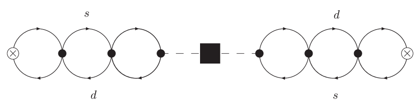
Figure 5.3: The leading $1/N_{c}$ contribution to $\Pi_{\Delta S=2}(q^{2})$ in our ladder resummation approximation. The crosses are insertions of the pseudoscalar current, $P^{ds}$, and the box is a $\Gamma_{\Delta S=2}$ insertion. The resummation in terms of bubbles leads to full two-point functions.

When the $X$ boson propagator is cut, as in (5.88), this diagram factorizes and gives the LO in $N_{c}$ result

$$\Pi_{\Delta S=2}(q^{2})=-2\,\Pi^{\mu}_{P}(-q)_{sd}\Pi_{\mu}^{P}(q)_{sd}\,.$$ (5.89)

For the two-point functions in (5.89) we can use the expressions in (5.1.1), (5.1.2) in the chiral limit and (5.1.3) out of the chiral limit. After performing the appropriate reduction of $\Pi_{\Delta S=2}(q^{2})$ in (5.89) to the matrix element in (2.15), these functions lead to the known $1/N_{c}$ result $\hat{B}_{K}=3/4$.

The NLO in the $1/N_{c}$ expansion contribution to $\Pi_{\Delta S=2}(q^{2})$ in our approximation can be related to the general four-point function

$$\Pi_{PLPL}^{\mu\nu}(p_{1},p_{2},p_{3})=i^{3}\int d^{4}x\int d^{4}y\int d^{4}z\,e^{ip_{1}\cdot x}e^{ip_{2}\cdot y}e^{ip_{3}\cdot z}\langle 0|P^{ds}(0)L^{\mu}_{sd}(x)P^{ds}(y)L^{\nu}_{sd}(z)|0\rangle\,,$$ (5.90)

with certain constraints in the moments and Lorentz indices. The left-handed currents are defined as $2L_{\mu}^{ij}=\bar{q}_{i}\gamma_{\mu}(1-\gamma_{5})q_{j}$.

In the case of four-point functions there are 2 classes of contributions within the method we are using: 3-point-functions like contributions and 4-point-functions like contributions. The former consists of two full 3-point functions with two sources each. They are obtained by gluing to the one-loop 3-point functions full 2-point function legs to obtain the full structure. Then the third leg of both full 3-point functions is removed and the two 3-point functions are pasted together with a propagator. This propagator can have any Dirac structure compatible with the strong interaction symmetries. The 4-point like functions contribution to the generalized four-point function consist in full four point functions with the same flavour and Dirac structure as the generalized four-point function we are calculating. Each of these full-four functions is constructed by gluing to the one-loop four-point function four sources with the full two-point functions permitted by the symmetries of the strong interactions that gives the required structure.

This implies the calculation of many one-loop four-point functions, as well as three-point functions with contributions from the chiral anomaly, such as $\Pi_{PVV}^{\mu\nu}(p_{1},p_{2})$ or $\Pi_{PAA}^{\mu\nu}(p_{1},p_{2})$. This method will allow us to calculate the $\Pi_{PLPL}^{\mu\nu}$ function analytically and investigate the cancellations between the different contributions coming from scalar, pseudoscalar, vector and axial-vector resonances. Work in progress is in this direction [166]. The first step, i.e., the calculation of $\hat{B}_{K}$ in the chiral limit to be compared with the results in [73] is expected to be finished soon.

5.7 An Example of OPE Green’s Function Calculation

The operator product expansion (OPE) of local operators was first formulated by Wilson [167], who proposed an expansion of the following form

$$\langle a|A(x)B(0)|b\rangle\stackrel{{\scriptstyle{x^{\mu}\to 0}}}{{\sim}}\langle a|\sum_{n}C_{n}(x)O_{n}(0)|b\rangle$$ (5.91)

where $A$, $B$ and $O_{n}$ are local operators. $C_{n}(x)$ are c-number functions which can have singularities of the form $(x^{2}-i\varepsilon x^{0})^{-p}$, with p being any real number and also involve logarithms of $x^{2}$. The functions $C_{n}(x-y)$ are determined, except for some constants, by scale invariance (if it is the case). They must be homogeneous functions of order $n-d(A)-d(B)$ in $(x-y)$ where $n$, $d(A)$ and $d(B)$ are the canonical dimensions of the operators $O_{n}$, $A$ and $B$ respectively.

In general, there is an infinite number of non-singular operators $O_{n}$ entering in an OPE; however, to a finite order in $x$ they reduce to a finite number. This kind of expansions are valid also for time ordered products, commutators or any others combination of elementary or composite local fields of a free theory as well as of a renormalized interacting field theory to all orders in perturbation theory.

In this Thesis we are interested in the OPE of Green’s functions constructed with two-quark densities and currents, and within the Standard Model. The simplest case is a two point function of the type

$$\Pi(q^{2}) \equiv i\,\int{\rm d}^{4}y\,e^{iy\cdot q}\,\langle 0|T\left[A(y)B(0)\right]|0\rangle\,,$$ (5.92)

where A and B are densities. An example of this kind of functions is $\Pi_{SS+PP}^{(a)}(p^{2})$, that appears in the calculation of the $\Delta I=3/2$ contribution to $\varepsilon_{K}^{\prime}$ (see Chapter 6). For euclidean values Q of the moment ($q^{2}=-Q^{2}$), for which $Q^{\mu}\to\infty$ implies $Q^{2}\to-\infty$, we can apply the expansion in (5.91) and pass strictly from the limit $x^{\mu}\to\infty$ to the limit $Q^{\mu}\to\infty$ in the next way

$$\lim_{Q\to\infty}\,\Pi(Q^{2}) = \sum_{n=0}^{\infty}\sum_{i=1}\,\langle 0|O_{2n}^{(i)}(0)|0\rangle(\nu)C_{2n}^{(i)}(\nu,Q^{2})\,,$$ (5.93)

with $O_{2n}$ gauge invariant operator of dimension 2n constructed from quark and gluon fields.

In the standard perturbative theory only the unit operator survive in the sum in (5.93). Non-vanishing values of the vacuum expectation values of operators of higher dimension, the so called condensates, are pure non-perturbative effects. Therefore, they correct the perturbative calculation by introducing terms of the type $(1/Q^{2})^{n}$ with $n\geq 1$. Once they are renormalized, the vacuum condensates depend on the renormalization scale $\nu$ in such a way that they cancel the scale dependence of the coefficients $C_{2n}^{(i)}(\nu,Q^{2})$ if the complete OPE is considered.

As an example of the calculation of the Wilson coefficients $C_{2n}^{(i)}(\nu,Q^{2})$, we briefly outline here the method followed to obtain the results in Appendix C. For detailed examples of this kind of calculations see [168]. We consider the combination of three-point functions

$$\Pi^{PAS+SAP}_{\mu}(p_{1},p_{2})\equiv\Pi^{PAS}_{\mu}(p_{1},p_{2})+\Pi^{SAP}_{\mu}(p_{1},p_{2})\,,$$ (5.94)

that is known to be an order parameter. The two functions $\Pi^{PAS}$ and $\Pi^{SAP}$ are defined as in (5.32). The first non-vanishing contribution to $\Pi^{PAS+SAP}_{\mu}(p_{1},p_{2})$ in the chiral limit, $\Pi^{(PAS+SAP)\,\chi}_{\mu}(p_{1},p_{2})$ is proportional to the quark condensate squared.

The diagrams contributing to this order in the OPE belong to one of the three groups showed in Figure 5.4. In total, we must calculate 18 diagrams for each of the three-point functions involved in the combination $\Pi^{(PAS+SAP)\,\chi}_{\mu}(p_{1},p_{2})$. Since it is quite a cumbersome task, we give here, only as an example, the calculation of the first diagram in Figure 5.4 for the function $\Pi^{PAS}_{\mu}(p_{1},p_{2})^{\chi}$, which we will denote by $\Pi^{PAS}_{\mu}(p_{1},p_{2})^{\chi}_{(1)}$ .

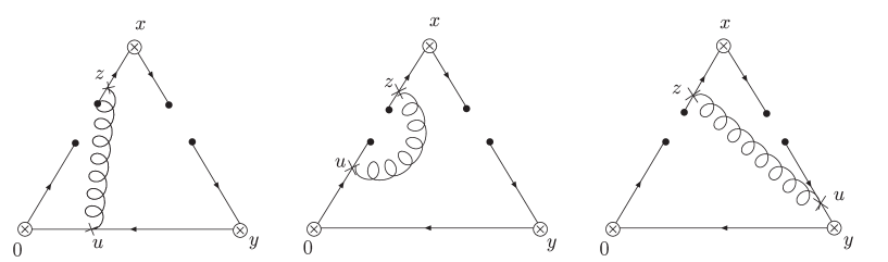
Figure 5.4: The three types of diagrams that contribute to the dominant term in the OPE of the function $\Pi^{PAS+SAP}_{\mu}(p_{1},p_{2})$. For explanations, see the text.

This diagram comes from the Green function with two insertion of the interacting lagrangian

$$i^{2}\frac{i^{2}}{2}\int d^{4}x\,d^{4}y\,d^{4}z\,d^{4}u\,e^{ip_{1}\cdot x}e^{ip_{2}\cdot y}\langle 0|T\left[P(0)A_{\mu}(x)S(y)L_{I}(z)L_{I}(u)\right]|0\rangle\,,$$ (5.95)

where

$$P(0) = :\bar{q}^{A}_{\alpha i}(0)\left(i\gamma_{5}\right)_{ij}q^{A}_{\alpha j}(0):\,,$$

$$A_{\mu}(x) = :\bar{q}^{B}_{\beta k}(x)\left(\gamma_{\mu}\gamma_{5}\right)_{kl}q^{B}_{\beta l}(x):\,,$$

$$S(y) = :\bar{q}^{C}_{\gamma}(y)(-1)q^{C}_{\gamma}(y):\,,$$

$$L_{I}(z) = \frac{1}{2}g:\bar{q}_{\delta m}^{D}(z)\lambda_{\delta\sigma}^{a}\left(\gamma_{\nu}\right)_{mn}q_{\sigma n}^{D}(z)B_{a}^{\nu}(z):\,,$$

$$L_{I}(u) = \frac{1}{2}g:\bar{q}_{\rho o}^{E}(u)\lambda_{\rho\eta}^{b}\left(\gamma_{\xi}\right)_{op}q_{\eta p}^{E}(u)B_{b}^{\xi}(u):\,.$$ (5.96)

In these definitions, the capital letters are flavour indices, the Greek letters are colour indices, $B_{b}^{\mu}(x)$ is a gluon field and $\lambda$ are the Gell-Mann matrices in colour space with

$$\lambda^{a}_{\delta\sigma}\lambda^{b}_{\rho\eta}=2\left[\delta_{\delta\eta}\delta_{\sigma\rho}-1/N_{c}\delta_{\delta\sigma}\delta_{\eta\rho}\right]\delta^{ab}\,.$$ (5.97)

Now we do in (5.95) the contractions of the fields corresponding to the first diagram, applying the relation in (5.97) and the definitions of the fermion and gluon propagators

$$q\mathop{\vtop{\halign{#\cr$\hfil\displaystyle{\kern 1.0pt^{A}_{\alpha i}(x)\bar{q}^{B}_{\beta j}\kern 1.0pt}\hfil$\crcr\kern 3.0pt\nointerlineskip\cr$\hbox{\vrule height=3.0pt,depth=0.0pt,width=1.0pt}\leaders\vrule\hfill\hbox{\vrule height=3.0pt,depth=0.0pt,width=1.0pt}$\crcr\kern 3.0pt\cr}}}\limits(y)\equiv i\delta_{AB}\delta_{ij}S_{ij}^{A}(x-y)\,,\quad\quad B\mathop{\vtop{\halign{#\cr$\hfil\displaystyle{\kern 1.0pt_{a}^{\nu}(z)B_{b}^{\xi}\kern 1.0pt}\hfil$\crcr\kern 3.0pt\nointerlineskip\cr$\hbox{\vrule height=3.0pt,depth=0.0pt,width=1.0pt}\leaders\vrule\hfill\hbox{\vrule height=3.0pt,depth=0.0pt,width=1.0pt}$\crcr\kern 3.0pt\cr}}}\limits(u)\equiv\delta_{ab}D_{\nu\xi}(z-u)\,,$$ (5.98)

that are given by

$$S^{A}_{ij}(x-y) = \int\frac{d^{4}k}{(2\pi)^{4}}S_{ij}^{A}(k)e^{-ik\cdot(x-y)}\,,\quad\quad S^{A}(k)\equiv\frac{1}{\not\!{\bf k}-m_{A}+i\eta}$$

$$D_{\mu\nu}(x-y) = \int\frac{d^{4}k}{(2\pi)^{4}}D_{\mu\nu}(k)e^{-ik\cdot(x-y)}\,,\quad D_{\mu\nu}(k)\equiv\frac{1}{k^{2}+i\eta}\left[-g_{\mu\nu}+(1-a)\frac{k_{\mu}k_{\nu}}{k^{2}+i\eta}\right]\,.$$

The result we obtain from the first diagram is then

$$\Pi^{PAS}_{\mu}(p_{1},p_{2})^{\chi}_{(1)} = \frac{i^{9}}{4}g^{2}\sum_{ABC}\int d^{4}x\,d^{4}y\,d^{4}z\,d^{4}u\,\int\frac{d^{4}k}{(2\pi)^{4}}\frac{d^{4}l}{(2\pi)^{4}}\frac{d^{4}v}{(2\pi)^{4}}\frac{d^{4}w}{(2\pi)^{4}}\frac{1}{k^{2}}(-g_{\nu\xi})$$

$$\times e^{ip_{1}\cdot x}e^{ip_{2}\cdot y}e^{-ik\cdot(z-u)}e^{il\cdot u}e^{-iv\cdot(u-y)}e^{-iw\cdot(x-z)}\left[\gamma_{5}S(l)^{A}\gamma_{\xi}S(v)^{C}\gamma_{\mu}\gamma_{5}S(w)^{B}\gamma_{\nu}\right]$$

$$\left\{\langle 0|:\bar{q}_{\sigma i}^{A}(0)\bar{q}_{\gamma k}^{B}(x)q_{\gamma r}^{A}(y)q_{\sigma n}^{B}(z):|0\rangle-\frac{1}{N_{c}}\langle 0|:\bar{q}_{\gamma i}^{A}(0)\bar{q}_{\sigma k}^{B}(x)q_{\gamma r}^{A}(y)q_{\sigma n}^{B}(z):|0\rangle\right\}.$$

After doing the trace of the Dirac matrices, this expression in the chiral limit simplifies to

$$\Pi^{PAS}_{\mu}(p_{1},p_{2})^{\chi}_{(1)} = \frac{i^{9}}{4}g^{2}\sum_{ABC}\frac{1}{p_{1}^{2}}\frac{-8(p_{1}^{2}p_{2}^{\mu}+p_{2}^{2}p_{1}^{\mu})}{p_{1}^{2}p_{2}^{2}(p_{1}+p_{2})^{2}}\,\frac{1}{144}\frac{1-N_{c}}{N_{c}}\langle\overline{q}q\rangle_{\chi}^{2}$$ (5.101)

$$= i\alpha_{s}\langle\overline{q}q\rangle_{\chi}^{2}\frac{18}{27}\frac{p_{1}^{2}p_{2}^{\mu}+p_{2}^{2}p_{1}^{\mu}}{p_{1}^{2}p_{2}^{2}(p_{1}+p_{2})^{2}}\,,$$

that is the final result for the contribution from the first diagram in Figure 5.4 for the PAS part of the dominant term in the OPE of $\Pi^{PAS+SAP}_{\mu}(p_{1},p_{2})^{\chi}$. The next step to get the final value in Appendix C will be to calculate the SAP part from this first diagram. Then, we will have to repeat the calculation for the other 17 diagrams.

Chapter 6 Hadronic Matrix Elements of the Electroweak Operators $Q_{7}$ and $Q_{8}$

In this chapter we report recent advances on the computation of the matrix elements of the electroweak penguins $Q_{7}$ and $Q_{8}$ which are relevant for the $\Delta I=3/2$ contribution to $\varepsilon^{\prime}_{K}$ in the chiral limit, as said in Section 2.4.2. These matrix elements can be calculated without using any model, but relating them with integrals over spectral functions for which there exist experimental data. This calculation is also an example of the use of the X-boson method at all orders in the $1/N_{C}$ expansion.

The method followed in the derivation of these matrix elements starts from the effective action (6.3) whose derivation from the Standard Model using short-distance renormalization group methods has been described in 2.4. In a general way

$$\Gamma_{SD}=\sum_{i=7,8}C_{i}(\mu_{R})Q_{i}(\mu_{R})\,.$$ (6.1)

This effective action can be used directly in lattice calculations but is less easy to use in other methods. What we know how to identify are currents and densities. We therefore go over to an equivalent scheme using only densities and currents whereby we generate (6.1) by the exchange of colourless $X$-bosons (Eq. (6.5))

$$\Gamma_{X}=\sum_{i}g_{i}(\mu_{C})X_{i}^{I}(\bar{q}^{\prime}\gamma_{I}q)$$ (6.2)

where the coupling constants $g_{i}$ can be determined using short-distance calculations only. The result is Eqs. (6.6) and (6.1). At this step the scheme-dependence in the calculation of the Wilson coefficients $C_{i}$ is removed but we have now a dependence on $M_{X}$ and the scheme used to calculate with $\Gamma_{X}$.

We then need to evaluate the matrix-elements of (6.2). For the case at hand this simplifies considerably. In the chiral limit, the relevant matrix element can be related to vacuum matrix elements (VEVs). The disconnected contributions are just two-quark condensates. The connected ones can be expressed as integrals over two-point functions (or correlators) as given in Eq. (6.1), which we evaluate in Euclidean space. The two relevant integrals are Eqs. (6.14) and (6.24).

Both of the integrals are now dealt with in a similar way. We split them into two pieces at a scale $\mu$ via Eq. (6.15). The two-point function to be integrated over is replaced by its spectral representation, which we assume known.

The long-distance part of the $Q^{2}$ integral can be evaluated and integrals of the type (6.17) and (6.34) remain.

The short-distance part we evaluate in a somewhat more elaborate way which allows us to show that the residual dependence on the $X$-boson mass disappears and that the correct behaviour given by the renormalization group is also incorporated. To do this, we split the short-distance integral in the part with the lowest dimensional operator, which is of dimension six for both $Q_{7}$ and $Q_{8}$, and the remainder, the latter is referred to as the contribution from higher-order operators [169].

The dimension six part can be evaluated using the known QCD short-distance behaviour of the two-point functions at this order. It is vacuum expectation values of dimension six operators over $Q^{6}$ for $Q_{7}$ and over $Q^{4}$ for $Q_{8}$ times a known function of $\alpha_{S}$. The vacuum expectation values can be rewritten again as integrals over two-point functions and the resulting integrals are precisely those needed to cancel the remaining $M_{X}$-dependence. For the contribution from all higher order operators we again perform simply the relevant $Q^{2}$ integrals over the same two-point functions as for dimension six and they are the ones needed to match long- and short-distances exactly.

This way we see how our procedure precisely cancels all the scheme- and scale-dependence and fully relates the results to known spectral functions.

The chapter consists out of two parts. In the first part, Sections 6.1–6.3, we discuss how the $X$-boson approach takes care of the scheme-dependence in the chiral limit independent of the large $N_{c}$ expansion we used in our previous work. We also show precisely how the needed matrix-elements in the chiral limit are related to integrals over spectral functions. This clarifies and extends the previous work on this relation [80, 81, 82, 170]. Equation (6.40) is our main result, but we also present the expression in terms of the usual bag parameters in Section 6.3.

In the second part, Sections 6.4–6.7, we present numerical results and compare our results with those obtained by others and our previous work. Sections 6.4 and 6.5 describe the experimental and theoretical information on both $\mbox{Im }\Pi_{LR}^{T}(Q^{2})$ and the scalar–pseudo-scalar $\mbox{Im }\Pi_{SS+PP}^{(0-3)}(Q^{2})$ spectral functions and give the values of the various quantities needed. The comparison with earlier results is Section 6.7.

In addition, in the Appendix A.1 we derive the NLO in $\alpha_{S}$ coefficient of the leading order term in the OPE of the needed correlators in the same scheme as used for the short-distance weak Hamiltonian. This coefficient was previously only known in a different scheme [171].

6.1 The $Q_{7}$ and $Q_{8}$ Operators

The imaginary part of $G_{E}$, the coupling defined in (3.1) that modulates the chiral Lagrangian of order $e^{2}p^{0}$, is dominated by the short-distance electroweak effects and can thus be reliably estimated from the purely strong matrix-elements of the $|\Delta S|=1$ effective hamiltonian in (2.30) with only the $Q_{7}$ and $Q_{8}$ operators present

$$\Gamma_{{\rm eff}} = -\frac{G_{F}}{\sqrt{2}}\,V_{ud}V_{us}^{*}\,{\displaystyle\sum_{i=7,8}}\,\mbox{Im }C_{i}\,\,\int{\rm d}^{4}x\,Q_{i}(x)$$ (6.3)

with $\mbox{Im }C_{i}=y_{i}\,\mbox{Im }\tau$ the imaginary part of the Wilson coefficients in (2.30). Up to $O(\alpha_{S}^{2})$, the $Q_{7}$ and $Q_{8}$ operators only mix between themselves below the charm quark mass via the strong interaction.

The QCD anomalous dimension matrix $\gamma(\nu)$ in regularizations like Naive Dimensional Regularization (NDR) or ’t Hooft-Veltman (HV) which do not mix operators of different dimension, is defined as ($i=$ 7,8)

$$\nu\,\frac{{\rm d}}{{\rm d}\nu}Q_{i}(\nu) = -{\displaystyle\sum_{j=7,8}}\gamma^{ji}(\nu)\,Q_{j}(\nu)\,;\quad\quad\gamma(\nu)=\sum_{n=1}\gamma^{(n)}a^{n}(\nu)\,$$ (6.4)

where $a(\nu)\equiv\alpha_{S}(\nu)/\pi$.

At low energies, it is convenient to describe the $\Delta S=1$ transitions with an effective action $\Gamma_{LD}$ which uses hadrons, constituent quarks, or other objects to describe the relevant degrees of freedom. A four-dimensional regularization scheme like an Euclidean cut-off, separating long-distance physics from integrated out short-distance physics, is also more practical. In addition, the color singlet Fierzed operator basis becomes useful for identifying QCD currents and densities. The whole procedure has been explicitly done in [75, 72] and reviewed in [172].

At low energies, the effective action (6.3) is therefore replaced by the equivalent

$$\Gamma_{X} = \ g_{7}(\mu_{C},\cdots)X_{7}^{\mu}\,\left((\overline{s}\gamma_{\mu}d)_{L}+\frac{3}{2}e_{q}{\displaystyle\sum_{q=u,d,s}}(\overline{q}\gamma_{\mu}q)_{R}\right)$$ (6.5)

$$+ g_{8}(\mu_{C},\cdots){\displaystyle\sum_{q=u,d,s}}X_{q,8}\left((\overline{q}d)_{L}+(-2)\frac{3}{2}e_{q}(\overline{s}q)_{R}\right)\,.$$

Here all colour sums are performed implicitly inside the brackets. There is also a kinetic term for the X-bosons which we take to be all of the same mass for simplicity.

The couplings $g_{i}$ are determined as functions of the Wilson coefficients $C_{i}$ by taking matrix elements of both sides between quark and gluon external states as explained in [75, 72, 172]. We obtain

$$\frac{|g_{7}(\mu_{C})|^{2}}{M_{X}^{2}} = \mbox{Im }C_{7}(\mu_{R})\,\left[1+a(\mu_{C})\,\left(\gamma^{(1)}_{77}\ln\frac{M_{X}}{\mu_{R}}+\Delta r_{77}\right)\right]$$ (6.6)

$$+ \mbox{Im }C_{8}(\mu_{R})\,\left[a(\mu_{C})\,\Delta r_{78}\right]+O\big{(}a(\mu_{R})-a(\mu_{C})\big{)}$$

and

$$\frac{|g_{8}(\mu_{C})|^{2}}{M_{X}^{2}} = \mbox{Im }C_{8}(\mu_{R})\,\left[1+a(\mu_{C})\,\left(\gamma^{(1)}_{88}\ln\frac{M_{X}}{\mu_{R}}+\tilde{\gamma}^{(1)}_{88}\ln\frac{\mu_{C}}{M_{X}}+\Delta r_{88}\right)\right]$$

$$+ \mbox{Im }C_{7}(\mu_{R})\,\left[a(\mu_{C})\,\left(\gamma^{(1)}_{87}\ln\frac{M_{X}}{\mu_{R}}+\Delta r_{87}\right)\right]+O\big{(}a(\mu_{R})-a(\mu_{C})\big{)}\,.$$

$\tilde{\gamma}_{ij}^{(1)}$ is due to the anomalous dimensions of the two-quark color-singlet densities or currents. It vanishes for conserved currents. In our case $\tilde{\gamma}_{88}^{(1)}=-2\gamma_{m}^{(1)}$, where $\gamma_{m}^{(1)}$ is the QCD anomalous dimension of the quark mass in the regularization used in (6.5). The values of $\Delta r_{ij}\equiv(r-\tilde{r})_{ij}$ have been calculated in [72].

The effective action to be used at low-energies is now specified completely. Notice that singlet color currents and densities are connected by the exchange of a colourless X-boson and therefore are well identified also in the low energy effective theories, and the finite terms which appear due to the correct identification of currents and densities.

The coupling $G_{E}$ is defined in the chiral limit so that we can use soft pion theorems to calculate the relevant matrix-elements, and relate them to a vacuum-matrix-element. For the contribution of $Q_{7}$ and $Q_{8}$, we obtain

$$-\frac{3}{5}\,e^{2}\,F_{0}^{6}\,\mbox{Im }G_{E} = -|g_{7}(\mu_{C},\cdots)|^{2}\,3\,\,i\,\int\frac{{\rm d}^{4}p_{X}}{(2\pi)^{4}}\,\frac{1}{p_{X}^{2}-M_{X}^{2}}\,g_{\mu\nu}\,\Pi_{LR}^{\mu\nu}(p_{X}^{2})$$

$$+ |g_{8}(\mu_{C},\cdots)|^{2}\,i\,\int\frac{{\rm d}^{4}p_{X}}{(2\pi)^{4}}\,\frac{1}{p_{X}^{2}-M_{X}^{2}}\,\left(\Pi_{SS+PP}^{(0)}(p_{X}^{2})-\Pi_{SS+PP}^{(3)}(p_{X}^{2})\right)\,.$$

Where $\Pi_{LR}^{\mu\nu}(p^{2})$ is the following two-point function in the chiral limit [170, 80]:

$$\Pi_{LR}^{\mu\nu}(p) \equiv \frac{1}{2}\,i\,\int{\rm d}^{4}y\,e^{iy\cdot p}\,\langle 0|T\left[L^{\mu}(y)R^{\nu\dagger}(0)\right]|0\rangle\equiv\left[p^{\mu}p^{\nu}-g^{\mu\nu}p^{2}\right]\Pi_{LR}^{T}(p^{2})$$ (6.9)

$$+ p^{\mu}p^{\nu}\Pi_{LR}^{L}(p^{2})\,.$$

In Eq. (6.1) we used the chiral limit so SU(3) chiral symmetry is exact. $L(R)^{\mu}=(\overline{u}\gamma^{\mu}d)_{L(R)}$ or $L(R)^{\mu}=(\overline{d}\gamma^{\mu}s)_{L(R)}$, $\Pi^{L}_{LR}(p^{2})$ vanishes and $\Pi_{SS+PP}^{(a)}(p^{2})$ is the two-point function

$$\Pi_{SS+PP}^{(a)}(p^{2}) \equiv i\,\int{\rm d}^{4}y\,e^{iy\cdot p}\,\langle 0|T\left[(S+iP)^{(a)}(y)(S-iP)^{(a)}(0)\right]|0\rangle$$ (6.10)

with

$$S^{(a)}(x) = -\overline{q}(x)\frac{\lambda^{(a)}}{\sqrt{2}}q(x),\,\,P^{(b)}(x)=\overline{q}(x)i\gamma_{5}\frac{\lambda^{(a)}}{\sqrt{2}}q(x)\,.$$ (6.11)

The 3 $\times$ 3 matrix $\displaystyle\lambda^{(0)}=\sqrt{2}\,{I}/{\sqrt{3}}$ and the rest are the Gell-Mann matrices normalized to $\mbox{tr}\left(\lambda^{(a)}\lambda^{(b)}\right)=2\delta^{ab}$. An alternative form for the last term in (6.1) is,

$$|g_{8}(\mu_{C},\cdots)|^{2}\,3\,i\,\int\frac{{\rm d}^{4}p_{X}}{(2\pi)^{4}}\,\frac{1}{p_{X}^{2}-M_{X}^{2}}\,\Pi_{SS+PP}^{(ds)}(p_{X}^{2})$$ (6.12)

with

$$\Pi_{SS+PP}^{(ds)}(p^{2})=i\,\int{\rm d}^{4}y\,e^{iy\cdot p}\,\langle 0|T\left[(\overline{d}d)_{L}(y)(\overline{s}s)_{R}(0)\right]|0\rangle$$ (6.13)

and $\left(\overline{q}q\right)_{L(R)}=\overline{q}(1-(+)\gamma_{5})q$.

6.2 Exact Long–Short-Distance Matching at NLO in $\alpha_{S}$

6.2.1 The $\mathbf{Q_{7}}$ Contribution

In Euclidean space, the term multiplying $|g_{7}|^{2}$ in the rhs of (6.1) can be written as

$$-\frac{9}{16\pi^{2}}\int^{\infty}_{0}{\rm d}Q^{2}\frac{Q^{4}}{Q^{2}+M_{X}^{2}}\,\Pi_{LR}^{T}(Q^{2})$$ (6.14)

with $Q^{2}=-q^{2}$. We split the integration into a short-distance and a long-distance part by

$$\int^{\infty}_{0}\,{\rm d}Q^{2} = \int^{\mu^{2}}_{0}\,{\rm d}Q^{2}+\int^{\infty}_{\mu^{2}}\,{\rm d}Q^{2}$$ (6.15)

with $M_{X}^{2}>>\mu^{2}$. In QCD, $\Pi_{LR}^{T}(Q^{2})$ obeys an unsubtracted dispersion relation

$$\Pi_{LR}^{T}(Q^{2}) = \int_{0}^{\infty}{\rm d}t\,\frac{1}{\pi}\frac{\mbox{Im }\Pi_{LR}^{T}(t)}{t+Q^{2}}\,.$$ (6.16)

$\mathbf{Q_{7}}$ Long-distance

Putting (6.16) in (6.14) and performing the integral up to $\mu^{2}$ gives

$$-\frac{9}{16\pi^{2}}\int_{0}^{\infty}dt\frac{t^{2}}{M_{X}^{2}}\ln\left(1+\frac{\mu^{2}}{t}\right)\frac{1}{\pi}{\mbox{Im }\Pi_{LR}^{T}(t)}+{\cal O}\left(\frac{\mu^{2}}{M_{X}^{4}}\right)\,,$$ (6.17)

with the use of the Weinberg Sum Rules [162], Eqs. (6.4).

$\mathbf{Q_{7}}$ Short-distance

At large $Q^{2}$ in the chiral limit, $\Pi_{LR}^{T}(Q^{2})$ behaves in QCD as [145]

$$\Pi_{LR}^{T}(Q^{2}) \to \sum_{n=0}^{\infty}\,\sum_{i=1}\,\frac{C^{(i)}_{2(n+3)}(\nu,Q^{2})}{Q^{2(n+3)}}\,\langle 0|O^{(i)}_{2(n+3)}(0)|0\rangle(\nu)$$ (6.18)

where $O^{(i)}_{2(n+3)}(0)$ are dimension $2(n+3)$ gauge invariant operators.

$$O^{(1)}_{6}(0) = \frac{1}{4}\,L^{\mu}(0)\,R_{\mu}(0)=\frac{1}{4}\left(\overline{s}\gamma^{\mu}d\right)_{L}(0)\left(\overline{d}\gamma_{\mu}s\right)_{R}(0)\,;$$

$$O^{(2)}_{6}(0) = (S+iP)^{(0)}(0)\,(S-iP)^{(0)}(0)-(S+iP)^{(3)}(0)\,(S-iP)^{(3)}(0)$$ (6.19)

$$= 3\,(\overline{d}d)_{L}(0)(\overline{s}s)_{R}(0)\,.$$

The coefficients $C_{6}^{(i)}(\nu,Q^{2})$ are related to the anomalous dimension matrix defined in (6.4). This can be used to obtain the NLO in $\alpha_{S}$ part of the coefficient with the same choice of evanescent operators as in [65, 69], calculations of the $\alpha_{S}^{2}$ term in other schemes and choices of evanescent operators are in[171]. Our calculation and results are in App. A.1. At the order we work we only need the lowest order [145]

$$C^{(1)}_{6}(\nu,Q^{2}) = -\frac{16\pi^{2}a(\nu)}{3}\gamma_{77}^{(1)}$$

$$C^{(2)}_{6}(\nu,Q^{2}) = \frac{8\pi^{2}a(\nu)}{9}\gamma_{87}^{(1)}$$ (6.20)

The values of the coefficients of the power corrections are physical quantities and can be determined with global duality FESR, [31, 137, 173],

$${\displaystyle\sum_{m=0}^{\infty}\,\sum_{i=1}}(-1)^{m}\,\langle 0|O^{(i)}_{2(m+3)}(0)|0\rangle(s_{0})\,\frac{1}{2\pi i}\,\oint_{C_{s_{0}}}\,{\rm d}s\,\frac{C^{(i)}_{2(m+3)}(s_{0},-s)}{s^{1+m-n}}$$

$$=M_{n+2}\equiv\int_{0}^{s_{0}}{\rm d}t\,t^{n+2}\,\frac{1}{\pi}\,\mbox{Im }\Pi_{LR}^{T}(t)\,,$$ (6.21)

with $n\geq 0$. $s_{0}$ is the threshold for local duality. At leading order in $\alpha_{S}$ only $n=m$ survive and we can rewrite the short-distance contribution to (6.14) as

$$-\frac{9}{16\pi^{2}}\int^{\infty}_{\mu^{2}}{\rm d}Q^{2}\frac{Q^{4}}{Q^{2}+M_{X}^{2}}\,\Pi_{LR}^{T}(Q^{2})=$$ (6.22)

$$= a(\mu)\,\ln\frac{\mu}{M_{X}}i\int\frac{{\rm d}^{4}\tilde{q}}{(2\pi)^{4}}\,\left(\frac{1}{M_{X}^{2}}\right)\,\,\left[\gamma^{(1)}_{77}\,3g_{\mu\nu}\,\Pi_{LR}^{\mu\nu}(\tilde{q})-\gamma^{(1)}_{87}\,\left(\Pi_{SS+PP}^{(0)}(\tilde{q}^{2})-\Pi_{SS+PP}^{(3)}(\tilde{q}^{2})\right)\right]$$

$$+\left(\frac{-1}{M_{X}^{2}}\right)\frac{9}{16\pi^{2}}\,\sum_{n=1}^{\infty}\frac{1}{n}\,\sum_{i=1}\frac{C^{(i)}_{2(n+3)}}{\mu^{2n}}\left[1+O\left(\frac{\mu^{2}}{M_{X}^{2}}\right)\right]\langle 0|O^{(i)}_{2(n+3)}(0)|0\rangle+O(a^{2})+\cdots$$

$$= a(\mu)\,\ln\frac{\mu}{M_{X}}i\int\frac{{\rm d}^{4}\tilde{q}}{(2\pi)^{4}}\,\left(\frac{1}{M_{X}^{2}}\right)\,\,\left[\gamma^{(1)}_{77}\,3g_{\mu\nu}\,\Pi_{LR}^{\mu\nu}(\tilde{q})-\gamma^{(1)}_{87}\,\left(\Pi_{SS+PP}^{(0)}(\tilde{q}^{2})-\Pi_{SS+PP}^{(3)}(\tilde{q}^{2})\right)\right]$$

$$+\frac{9}{16\pi^{2}}\,\int_{0}^{s_{0}}{\rm d}t\,\frac{t^{2}}{M_{X}^{2}}\,\ln\left(1+\frac{t}{\mu^{2}}\right)\,\frac{1}{\pi}\,\mbox{Im }\Pi^{T}_{LR}(t)+{\cal O}\left(\frac{\mu^{2}}{M_{X}^{4}}\right)+{\cal O}(a^{2})$$

where we have used

$$\int\frac{{\rm d}^{4}\tilde{q}}{(2\pi)^{4}}\,\int{\rm d}^{4}x\,e^{ix\cdot\tilde{q}}\,\langle 0|T\left[J(x)\,\tilde{J}(0)\right]|0\rangle \equiv \langle 0|J(0)\,\tilde{J}(0)|0\rangle\,.$$ (6.23)

6.2.2 The $\mathbf{Q_{8}}$ Contribution

In Euclidean space, the term multiplying $|g_{8}|^{2}$ in the rhs of (6.1), is

$$\frac{1}{16\pi^{2}}\int^{\infty}_{0}{\rm d}Q^{2}\frac{Q^{2}}{Q^{2}+M_{X}^{2}}\,\Pi_{SS+PP}^{(0-3)}(Q^{2})\,$$ (6.24)

with

$$\Pi_{SS+PP}^{(0)}(Q^{2})-\Pi_{SS+PP}^{(3)}(Q^{2}) \equiv \Pi_{SS+PP}^{(0-3)}(Q^{2})\,.$$ (6.25)

This two-point function has a disconnected contribution, corresponding to what is usually called the factorizable contribution. We split off that part explicitly:

$$\frac{1}{16\pi^{2}}\int^{\infty}_{0}{\rm d}Q^{2}\frac{Q^{2}}{Q^{2}+M_{X}^{2}}\,\Pi_{SS+PP}^{(0-3)}(Q^{2})\,=\frac{1}{M_{X}^{2}}\,\big{|}\langle 0|S^{(0)}(0)|0\rangle\big{|}^{2}\,$$

$$+\frac{1}{16\pi^{2}}\int^{\infty}_{0}{\rm d}Q^{2}\frac{Q^{2}}{Q^{2}+M_{X}^{2}}\,\Pi_{SS+PP}^{(0-3)~{}conn}(Q^{2})\,.$$ (6.26)

The Disconnected Contribution

We have included in (6.1) all the $O(\alpha_{S})$ logs and finite terms that take into account passing the four-quark matrix element from the cut-off $\mu_{C}$ regulated $X$-boson effective theory to the $\overline{MS}$ one. Therefore to the order needed

$$\langle 0|S^{(0)}(0)|0\rangle^{2}=3\,\langle 0|\overline{q}q|0\rangle\big{|}^{2}_{\overline{MS}}(\mu_{C})$$ (6.27)

and from now on the quark condensate is understood to be in the $\overline{MS}$ scheme. As shown in [174, 175], $\gamma_{88}^{(1)}=-2\gamma_{m}^{(1)}$ where $\gamma_{m}^{(1)}$ is the one-loop quark mass anomalous dimension. This cancels exactly the scale $\mu_{C}$ dependence in (6.1) to order $\alpha_{S}$[174, 175].

The disconnected contribution to $\mbox{Im }G_{E}$ is thus

$$-\frac{3}{5}\,e^{2}F_{0}^{6}\,\mbox{Im }G_{E}^{Fact}=3\,\langle 0|\bar{q}q|0\rangle^{2}(\mu_{C})\frac{|g_{8}(\mu_{C})|^{2}}{M_{X}^{2}}$$ (6.28)

but now with

$$\frac{|g_{8}(\mu_{C})|^{2}}{M_{X}^{2}} = \mbox{Im }C_{8}(\mu_{R})\left[1+a(\mu_{C})\left(\gamma^{(1)}_{88}\ln\frac{\mu_{C}}{\mu_{R}}+\Delta r_{88}\right)\right]$$ (6.29)

$$+ \mbox{Im }C_{7}(\mu_{R})a(\mu_{R})\left(\gamma^{(1)}_{87}\ln\frac{M_{X}}{\mu_{R}}+\Delta r_{87}\right)+{\cal O}(a^{2})\,.$$

Here one can see that the factorizable contribution is not well defined. It is due to the mixing of $Q_{7}$ and $Q_{8}$ and is reflected here in the $\ln(M_{X}/\mu_{R})$. This $M_{X}$ dependence cancels with the non-factorizable contribution of $Q_{7}$ in (6.22). Notice that the contribution of both terms, $\mbox{Im }C_{8}$ and $\mbox{Im }C_{7}$, to $\mbox{Im }G_{E}$ are of the same order in $1/N_{c}$. It is then necessary to add the non-factorizable term to have $\mbox{Im }G_{E}$ well defined. Since $\mbox{Im }G_{E}$ is a physical quantity, factorization is not well defined for $Q_{8}$. This was also shown to be the case for $Q_{6}$ in [74]. Of course, the leading term of the $1/N_{c}$ expansion is well defined but that approximation would miss a completely new topology, namely the non-factorizable contributions.

The Connected Contribution

From the leading high energy behaviour, the scalar–pseudo-scalar spectral functions satisfy in the chiral limit [5, 176]

$$\int_{0}^{\infty}dt\,\frac{1}{\pi}\,\left[\mbox{Im }\Pi_{SS}^{(0)}(t)-\mbox{Im }\Pi_{PP}^{(3)}(t)\right]=0=\int_{0}^{\infty}dt\,\frac{1}{\pi}\,\left[\mbox{Im }\Pi_{SS}^{(3)}(t)-\mbox{Im }\Pi_{PP}^{(0)}(t)\right]$$ (6.30)

which are analogous to Weinberg Sum Rules. Therefore the connected part of $\Pi^{(0-3)}_{SS+PP}(Q^{2})$ satisfies an unsubtracted dispersion relation in the chiral limit,

$$\Pi^{(0-3)\,\rm conn}_{SS+PP}(Q^{2})={\displaystyle\int^{\infty}_{0}}{\rm d}t\,\frac{1}{\pi}\,\frac{\mbox{Im }\Pi^{(0-3)}_{SS+PP}(t)}{t+Q^{2}}\,.$$ (6.31)

Also in the chiral limit, the scalar and pseudo-scalar $(0-3)$ combinations satisfy other Weinberg-like Sum Rules as shown in [177] for the scalar and in [178] for the pseudo-scalar,

$$\int_{0}^{\infty}dt\,\frac{1}{\pi}\,\mbox{Im }\Pi_{SS}^{(0-3)}(t)=0=\int_{0}^{\infty}dt\,\frac{1}{\pi}\,\mbox{Im }\Pi_{PP}^{(0-3)}(t)\,.$$ (6.32)

We also know that the spectral functions $\mbox{Im }\Pi_{SS(PP)}(Q^{2})$ depend on scale due to the non-conservation of the quark densities.

$$\mu_{C}\frac{{\rm d}}{{\rm d}\mu_{C}}\,\mbox{Im }\Pi_{SS(PP)}^{(a)}(t) = 2\gamma_{m}(\mu_{C})\,\mbox{Im }\Pi_{SS(PP)}^{(a)}(t)\,.$$ (6.33)

This scale dependence is analogous to the one of the disconnected part (6.28) and cancels the $\mu_{C}$ dependence in $|g_{8}(\mu_{C})|^{2}$ also for the connected part.

We now proceed as for $Q_{7}$ and split the integral in (6.2.2) at $\mu^{2}$.

6.2.2.a $\mathbf{Q_{8}}^{conn}$ Long-Distance

We perform simply the integral and obtain

$$-\frac{1}{16\pi^{2}}\int_{0}^{\infty}dt\frac{t}{M_{X}^{2}}\ln\left(1+\frac{\mu^{2}}{t}\right)\frac{1}{\pi}{\mbox{Im }\Pi_{SS+PP}^{(0-3)}(t)}+{\cal O}\left(\frac{\mu^{2}}{M_{X}^{4}}\right)\,.$$ (6.34)

6.2.2.b $\mathbf{Q_{8}}^{conn}$ Short-distance

Using the unsubtracted dispersion relation in (6.31), $\Pi_{SS+PP}^{(0-3)\,\rm conn}(Q^{2})$ in the chiral limit behaves at large $Q^{2}$ in QCD as

$$\Pi_{SS+PP}^{(0-3)\,\rm conn}(Q^{2}) \to \sum_{n=0}^{\infty}\,\sum_{i=1}\,\frac{\tilde{C}^{(i)}_{2(n+3)}(\nu,Q^{2})}{Q^{2(n+2)}}\,\langle 0|\tilde{O}^{(i)\rm}_{2(n+3)}(0)|0\rangle(\nu)$$ (6.35)

where $\tilde{O}^{(i)}_{2(n+3)}(0)$ are dimension $2(n+3)$ gauge invariant operators.

$$\tilde{O}^{(1)}_{6}(0)=O^{(1)}_{6}(0)\,;\quad\quad\tilde{O}^{(2)}_{6}(0)=O^{(2)}_{6}(0)\,.$$ (6.36)

Using the information on the mixing of $Q_{7}$ and $Q_{8}$ in (6.4), the scale dependence (6.33), it is easy to obtain the leading power behavior in (6.35) (see Appendix A.2)

$$\tilde{C}^{(1)}_{6}(\nu,Q^{2}) = \frac{45\pi^{2}}{2}a(\nu)^{2}+O(a^{3})\,;$$

$$\tilde{C}^{(2)}_{6}(\nu,Q^{2}) = \frac{211\pi^{2}}{4}a(\nu)^{2}+O(a^{3})\,.$$ (6.37)

Again the values of the coefficients of the power corrections in (6.35) can be calculated using global duality FESR,

$${\displaystyle\sum_{m=0}^{\infty}\,\sum_{i=1}}(-1)^{m+1}\langle 0|\tilde{O}^{(i)}_{2(m+3)}(0)|0\rangle(\tilde{s}_{0})\,\frac{1}{2\pi i}\,\oint_{C_{\tilde{s}_{0}}}{\rm d}s\,\frac{\tilde{C}^{(i)}_{2(m+3)}(\tilde{s}_{0},-s)}{s^{1+m-n}}$$

$$=\tilde{M}_{n+1}\equiv\int_{0}^{\tilde{s}_{0}}{\rm d}t\,t^{n+1}\,\frac{1}{\pi}\,\mbox{Im }\Pi^{(0-3)}_{SS+PP}(t)\,,$$ (6.38)

with $n\geq 0$, and $\tilde{s}_{0}$ the threshold for local duality for this two-point function. Again only terms with $n=m$ survive at $O(\alpha_{S})$ and one gets

$$\frac{1}{16\pi^{2}}\int^{\infty}_{\mu^{2}}{\rm d}Q^{2}\frac{Q^{2}}{Q^{2}+M_{X}^{2}}\,\Pi_{SS+PP}^{(0-3)~{}conn}(Q^{2})=$$ (6.39)

$$\frac{1}{16\pi^{2}}\,\int_{0}^{\tilde{s}_{0}}{\rm d}t\,\frac{t}{M_{X}^{2}}\,\ln\left(1+\frac{t}{\mu^{2}}\right)\,\frac{1}{\pi}\,\mbox{Im }\Pi^{(0-3)}_{SS+PP}(t)+{\cal O}\left(\frac{\mu^{2}}{M_{X}^{4}}\right)+{\cal O}(a^{3}).$$

6.2.3 Sum

We now add all the contributions of Eqs. (6.17), (6.22), (6.28), (6.34) and (6.39) to obtain the full result. Notice in particular that all contributions contain the correct logarithms of $M_{X}$ to cancel that dependence in Eqs. (6.6) and (6.1).

The integrals over the spectral functions in the respective long and short-distance regime can in both cases be combined to give a simple $\ln(t/\mu^{2})$.

Therefore, when summing everything to ${\cal O}(\alpha_{S})$ and all orders in $1/N_{c}$, we obtain

$$-\frac{3}{5}\,e^{2}F_{0}^{6}\mbox{Im }G_{E} = \Bigg{\{}\mbox{Im }C_{7}(\mu_{R})\left[1+a(\mu_{C})\left(\gamma^{(1)}_{77}\ln\frac{\mu}{\mu_{R}}+\Delta r_{77}\right)\right]$$ (6.40)

$$+\mbox{Im }C_{8}(\mu_{R})a(\mu_{C})\Delta r_{78}\Bigg{\}}\frac{9}{16\pi^{2}}{\cal A}_{LR}(\mu)$$

$$+ \left\{\mbox{Im }C_{8}(\mu_{R})\left[1+a(\mu_{C})\left(\gamma^{(1)}_{88}\ln\frac{\mu_{C}}{\mu_{R}}+\Delta r_{88}\right)\right]\right.$$

$$+\left.\mbox{Im }C_{7}(\mu_{R})a(\mu_{C})\left(\gamma^{(1)}_{87}\ln\frac{\mu}{\mu_{R}}+\Delta r_{87}\right)\right\}\times$$

$$\quad\times\left(3\,\langle 0|\bar{q}q|0\rangle^{2}(\mu_{C})+\frac{1}{16\pi^{2}}{\cal A}_{SP}(\mu,\mu_{C}))\right)\,;$$

where

$${\cal A}_{LR}(\mu) \equiv \int_{0}^{s_{0}}{\rm d}t\,t^{2}\,\ln\left(\frac{t}{\mu^{2}}\right)\,\frac{1}{\pi}\,\mbox{Im }\Pi^{T}_{LR}(t)\,;$$

$${\cal A}_{SP}(\mu,\mu_{C}) \equiv \int_{0}^{\tilde{s}_{0}}{\rm d}t\,t\ln\left(\frac{t}{\mu^{2}}\right)\frac{1}{\pi}\mbox{Im }\Pi_{SS+PP}^{(0-3)}(t)\,.$$ (6.41)

To obtain this result we have used the local duality relations

$$\int^{\infty}_{s_{0}}{\rm d}t\,t^{2}\,\ln\left(\frac{t}{\mu^{2}}\right)\,\frac{1}{\pi}\,\mbox{Im }\Pi^{T}_{LR}(t) = O(a^{2})\,,$$

$$\int^{\infty}_{\tilde{s}_{0}}{\rm d}t\,t\,\ln\left(\frac{t}{\mu^{2}}\right)\,\frac{1}{\pi}\,\mbox{Im }\Pi^{(0-3)}_{SS+PP}(t) = O(a^{2})\,.$$ (6.42)

The expression in (6.40) is exact in the chiral limit, at NLO in $\alpha_{S}$, all orders in $1/N_{c}$ and without electromagnetic corrections. It doesn’t depend on any scale nor scheme at that order analytically. The dependence on $M_{X}$ also nicely cancels out. The $\mu_{C}$ dependence cancels against the $\mu_{C}$ dependence of the densities. Notice that in this final result we have taken into account the contribution of all higher order operators.

As noticed in [72], the connected scalar–pseudo-scalar two-point function is exactly zero in U(3) symmetry, i.e. is $1/N_{c}$ suppressed. We used this fact to disregard this contribution there. We will check later the quality of this approximation from a phenomenological analysis of its value.

6.3 Bag Parameters

We now re-express our main result (6.40) in terms of the usual definition of the bag parameters

$$-\frac{3}{5}\,e^{2}F_{0}^{6}\mbox{Im }G_{E} \equiv \langle 0|\bar{q}q|0\rangle^{2}(\mu_{C})\left[\mbox{Im }C_{7}(\mu_{R})B_{7\chi}(\mu_{C},\mu_{R})+3\mbox{Im }C_{8}(\mu_{R})\,B_{8\chi}(\mu_{C},\mu_{R})\right]$$ (6.43)

$$\equiv -6\,\mbox{Im }C_{7}(\mu_{R})\,\langle 0|O_{6}^{(1)}|0\rangle_{\chi}(\mu_{R})+\mbox{Im }C_{8}(\mu_{R})\,\langle 0|O_{6}^{(2)}|0\rangle_{\chi}(\mu_{R})\,,$$

where the subscript $\chi$ means in the chiral limit.

This definition coincides with the one in [72] and gives

$$B_{7\chi}(\mu_{C},\mu_{R}) = \left[1+\Delta r_{77}\,a(\mu_{R})\right]\,\frac{9}{16\pi^{2}}\,\frac{1}{\langle 0|\bar{q}q|0\rangle^{2}(\mu_{C})}\,{\cal A}_{LR}(\mu_{R})$$

$$+ 3\,a(\mu_{C})\,\Delta r_{87}\left[1+\frac{1}{48\pi^{2}}\,\frac{1}{\langle 0|\bar{q}q|0\rangle^{2}(\mu_{C})}\,{\cal A}_{SP}(\mu_{R},\mu_{C})\right]\,;$$

$$B_{8\chi}(\mu_{C},\mu_{R}) = \left[1+\left(\gamma^{(1)}_{88}\ln\left(\frac{\mu_{C}}{\mu_{R}}\right)+\Delta r_{88}\right)a(\mu_{C})\right]\times$$ (6.44)

$$\times\left[1+\frac{1}{48\pi^{2}}\,\frac{1}{\langle 0|\bar{q}q|0\rangle^{2}(\mu_{C})}\,{\cal A}_{SP}(\mu_{R},\mu_{C})\right]$$

$$+ \frac{a(\mu_{C})}{\langle 0|\bar{q}q|0\rangle^{2}(\mu_{C})}\,\Delta r_{78}\,\frac{3}{16\pi^{2}}\,{\cal A}_{LR}(\mu_{R})\,.$$

The finite terms that appear in the matching between the X-boson effective theory with a cut-off and the Standard Model regularized with the NDR scheme were calculated in [72],

$$\Delta r^{\rm NDR}_{77}=\frac{1}{8N_{c}}\,,\quad\Delta r^{\rm NDR}_{78}=-\frac{3}{4}\,,\Delta r^{\rm NDR}_{87}=-\frac{1}{8}\,,\quad\Delta r^{\rm NDR}_{88}=\frac{5}{8}N_{c}+\frac{1}{8N_{c}}\,.$$ (6.45)

The finite terms to pass from NDR to HV in the same basis and evanescent operators we use can be found in [66]. In the HV scheme of [65, 69] these finite terms are

$$\Delta r^{\rm HV-NDR}_{77}=-\frac{3}{2N_{c}}\,,\quad\Delta r^{\rm HV-NDR}_{78}=1\,,\Delta r^{\rm HV-NDR}_{87}=\frac{3}{2}\,,\quad\Delta r^{\rm HV-NDR}_{88}=\frac{N_{c}}{2}-\frac{3}{2N_{c}}\,.$$ (6.46)

The results for the scheme dependent terms $\Delta r_{77}$ and $\Delta r_{87}$ [72] agree with those in [80, 82].

The $B_{7}$ and $B_{8}$ bag parameters are independent of $\mu$ but depend on $\mu_{R}$ and $\mu_{C}$, and these dependences only cancel in the physical value of $\mbox{Im }G_{E}$. The $\mu_{C}$ dependence is artificial and a consequence of the normalization of the bag parameters to the quark condensate.

At NLO in $1/N_{c}$ we get

$$B^{NDR}_{7\chi}(\mu_{C},\mu_{R}) = \left(1+\frac{a(\mu_{R})}{24}\right)\frac{9}{16\pi^{2}}\,\frac{1}{\langle 0|\bar{q}q|0\rangle^{2}(\mu_{C})}{\cal A}_{LR}(\mu_{R})$$

$$- \frac{3}{8}\,a(\mu_{C})\left[1+\frac{1}{48\pi^{2}}\frac{1}{\langle 0|\bar{q}q|0\rangle^{2}(\mu_{C})}\,{\cal A}_{SP}(\mu_{R},\mu_{C})\right]\,;$$

$$B^{NDR}_{8\chi}(\mu_{C},\mu_{R}) = \left[1+\frac{1}{12}\,\left(54\ln\left(\frac{\mu_{C}}{\mu_{R}}\right)+23\right)a(\mu_{C})\right]\times$$ (6.47)

$$\times\left[1+\frac{1}{48\pi^{2}}\frac{1}{\langle 0|\bar{q}q|0\rangle^{2}(\mu_{C})}{\cal A}_{SP}(\mu_{R},\mu_{C})\right]$$

$$- \,\frac{9}{64\pi^{2}}\,\,\frac{a(\mu_{R})}{\langle 0|\bar{q}q|0\rangle^{2}(\mu_{C})}{\cal A}_{LR}(\mu_{R})$$

and in the HV scheme[65, 69]

$$B^{HV}_{7\chi}(\mu_{C},\mu_{R}) = \left(1-\frac{11}{24}a(\mu_{R})\right)\frac{9}{16\pi^{2}}\,\frac{1}{\langle 0|\bar{q}q|0\rangle^{2}(\mu_{C})}\,{\cal A}_{LR}(\mu_{R})$$

$$+ \frac{33}{8}\,a(\mu_{C})\left[1+\frac{1}{48\pi^{2}}\frac{1}{\langle 0|\bar{q}q|0\rangle^{2}(\mu_{C})}{\cal A}_{SP}(\mu_{R},\mu_{C})\right]\,;$$

$$B^{HV}_{8\chi}(\mu_{C},\mu_{R}) = \left[1+\frac{1}{12}\,\left(54\ln\left(\frac{\mu_{C}}{\mu_{R}}\right)+35\right)a(\mu_{C})\right]\,\times$$ (6.48)

$$\times\left[1+\frac{1}{48\pi^{2}}\frac{1}{\langle 0|\bar{q}q|0\rangle^{2}(\mu_{C})}{\cal A}_{SP}(\mu_{R},\mu_{C})\right]$$

$$+ \frac{3}{64\pi^{2}}\,\frac{a(\mu_{R})}{\langle 0|\bar{q}q|0\rangle^{2}(\mu_{C})}{\cal A}_{LR}(\mu_{R})\,.$$

We find an exact result for these B-parameters in QCD in the chiral limit including the effects of higher dimensional operators to all orders. The scheme dependence is also fully taken into account. To our knowledge this is the first time these fully model independent expressions bag parameters are presented.

6.4 The $\,\Pi_{LR}^{T}(Q^{2})\,$ Two-Point Function and Integrals over It

There are very good data for $\Pi_{LR}^{T}$ [31, 137] in the time-like region below the tau lepton mass. They have been extensively used previously [80, 81, 179, 180], see the talks [173] for recent reviews. We consider it a good approximation to take this data as the chiral limit data. Nevertheless, one can estimate the effect of the chiral corrections with Cauchy’s integrals around a circle of radius $4m_{\pi}^{2}$ of the type

$$\oint_{4m_{\pi}^{2}}{\rm d}s\,s^{n}\,\ln^{m}(s)\,\Pi_{LR}^{T}(-s)\,$$ (6.49)

with $n>0$, $m=0,1$. For all the integrals we use, we have checked that these contributions are negligible using the CHPT expressions for $\Pi_{LR}^{T}(Q^{2})$ at one-loop[5]. The discussion below is focused on the ALEPH data but we present the OPAL results as well.

We reanalyze here the first and the second Weinberg Sum Rules (WSRs) [162], which are properties of QCD in the chiral limit [181],

$$\int_{0}^{\infty}{\rm d}t\,\frac{1}{\pi}\,\mbox{Im }\Pi_{LR}^{T}(t)=\int_{0}^{s_{0}}{\rm d}t\,\frac{1}{\pi}\,\mbox{Im }\Pi_{LR}^{T}(t)+O(a^{2})=f_{\pi}^{2}\,;$$

$$\int_{0}^{\infty}{\rm d}t\,t\,\frac{1}{\pi}\,\mbox{Im }\Pi_{LR}^{T}(t)=\int_{0}^{s_{0}}{\rm d}t\,t\,\frac{1}{\pi}\,\mbox{Im }\Pi_{LR}^{T}(t)+O(a^{2})=0\,$$ (6.50)

where we used the perturbative QCD result for the imaginary part at energies larger than $s_{0}$, i.e. we assumed local duality above $s_{0}$. These two WSRs determine the threshold of perturbative QCD $s_{0}$. We used the experimental value for the pion decay constant $f_{\pi}=(92.4\pm 0.4)$ MeV.

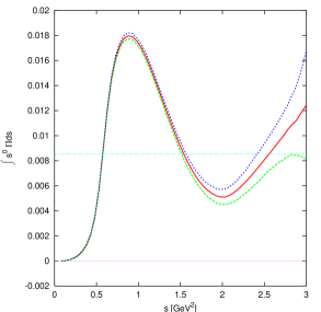
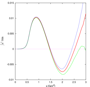
Figure 6.1: The first and second Weinberg sum rule as a function of the upper integration variable $s$. The central curve corresponds to the central values of [31] while the upper and lower curve are the one sigma errors calculated as described in the text.

These two sum rules are plotted in Fig. 6.1 for the central data values and the one sigma errors. These latter are calculated by generating a distribution of spectral functions distributed according to the covariance matrix of [31]. We then take the one sigma error to be the value where 68% of the distributions fall within. All errors in the numbers of this section and in the plots shown are calculated in this way.

At this point, we would like to discuss where local duality sets in: $s_{0}$. As we can see from Fig. 6.1 for $s<M_{\tau}^{2}$ there are two points where (6.4) are satisfied, the first one around 1.5 GeV² and the second around 2.5 GeV². Of course, this does not mean that local duality is already settled at these points as the oscillations show. One can expect however that the violations of local duality are small at these points. It is also obvious that local duality will be better when the value of $s_{0}$ is larger. The procedure to determine the value of $s_{0}$ is repeated for each of the spectral functions generated before and we use consistently a spectral function together with its value of the onset of local duality.

There are several points worth making. Though for every distribution the first duality point in the 1st WSR is very near the corresponding one of the 2nd WSR, they differ by more than their error. Numerically, when used in other sum-rules they produce results outside the naive error. The second duality point, $s_{0}\approx 2.5$ GeV² yields more stable results. There is no a priori reason for the value of $s_{0}$ to be exactly the same for different sum rules.

Though the change from the 1st WSR to the second is small, and even smaller if one looks at negative moments, when one uses large positive moments (the ones we need here), the deviations are quite sizable as we will show. This is because positive large moments weigh more the higher energy region and the negative moments essentially use only information of the low energy region.

Probably in the second duality point, local duality has not been reached either but certainly we should be closer to the asymptotic regime. We therefore take the highest global duality point available, the solution of Eq. (6.4), around $2.5~{}$GeV². Fortunately, for the physical matrix elements, the additional $\log(t/\mu^{2})$ in the integrand reduces the contribution of the data points near the real axis for $t$ around $\mu^{2}$. This makes these sum rules much more reliable than the single moments used in [80, 81].

The second, and highest value with good data, value of $s_{0}$ where the WSRs are satisfied runs roughly between 2.2 GeV² and 3.0 GeV². But not all of these values are equally probable. If we look at the distribution of the $s_{0}$ values, there is a clear peak situated around the value calculated with the central data points but there are tails towards higher $s_{0}$. The widths of the peak are essentially the same as the errors we quote. The $s_{0}$ where the second WSR are mainly in the area

$$s_{0} = (2.53^{+0.13}_{-0.12})\,{\rm GeV}^{2}~{}\mbox{(ALEPH)}\,,\quad\quad s_{0}=(2.49^{+0.17}_{-0.13})\,{\rm GeV}^{2}~{}\mbox{(OPAL)}\,.$$ (6.51)

and where the first WSR is satisfied in

$$s_{0} = (2.56^{+0.15}_{-0.14})\,{\rm GeV}^{2}~{}\mbox{(ALEPH)}\,,\quad\quad s_{0}=(2.53^{+0.17}_{-0.12})\,{\rm GeV}^{2}~{}\mbox{(OPAL)}\,.$$ (6.52)

These errors have been obtained as explained above. In the analysis below we use all experimental distributions with their associated value of $s_{0}$ and not only those with $s_{0}$ in the intervals above.

The OPE of the $\Pi_{LR}^{T}(Q^{2})$ was studied using the same data [31] in [179]. They obtained a quite precise determination of the dimension six and eight higher dimensional operators from a fit to different moments of the energy distribution. This procedure has in principle smaller errors since one can use the tau decay kinematic factors which suppresses the data near the real axis but has a different local duality error. They use $M_{\tau}^{2}$ as upper limit of the hadronic moments, we agree with [180] that one should use the $s_{0}$ where there is global duality with QCD to eliminate possible effects of the lack of local duality at $M_{\tau}^{2}$. Another comment is that as noticed in [82] the $\alpha_{S}^{2}$ corrections used in [179] are in a different scheme [171]. These corrections in the scheme used in [69] are presented in the appendices.

We can determine the following higher dimensional operator contributions (6.18)

$$M_{2} \equiv \int_{0}^{s_{0}}{\rm d}t\,t^{2}\,\frac{1}{\pi}\,\mbox{Im }\Pi_{LR}^{T}(t)$$

$$= {\displaystyle\displaystyle\sum_{m=0}^{\infty}\,\sum_{i=1}}\langle 0|O^{(i)}_{2(m+3)}(0)|0\rangle(s_{0})\,(-1)^{m}\,\frac{1}{2\pi i}\,\oint_{C_{s_{0}}}\,{\rm d}s\,\frac{C^{(i)}_{2(m+3)}(s_{0},-s)}{s^{1+m}}\,$$

$$M_{3} \equiv \int_{0}^{s_{0}}{\rm d}t\,t^{3}\,\frac{1}{\pi}\,\mbox{Im }\Pi_{LR}^{T}(t)$$ (6.53)

$$= {\displaystyle\displaystyle\sum_{m=0}^{\infty}\,\sum_{i=1}}\langle 0|O^{(i)}_{2(m+3)}(0)|0\rangle(s_{0})\,(-1)^{m}\,\frac{1}{2\pi i}\,\oint_{C_{s_{0}}}\,{\rm d}s\,\frac{C^{(i)}_{2(m+3)}(s_{0},-s)}{s^{m}}\,.$$

In Fig. 6.2 we have plotted the value of $M_{2}$ and $M_{3}$ as a function of $s_{0}$ used in the integration, together with the one sigma error band. It is immediately obvious that the main uncertainty is the choice of $s_{0}$ to be used. This uncertainty is increasingly important with the increase of the moment.

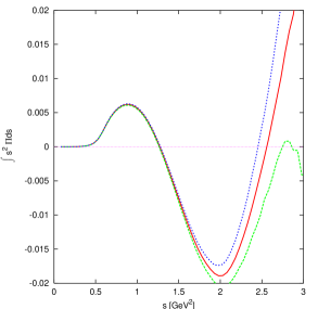
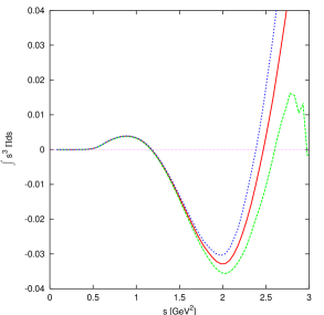
Figure 6.2: The second and third moment as a function of the upper limit of integration $s_{0}$ and the one sigma variation.

Using ALEPH data on $V-A$ spectral functions we get for the dimension six and eight FESR using the value for $s_{0}$ where the second WSR is satisfied

$$M_{2} = -(1.7^{+1.2}_{-1.0})\cdot 10^{-3}\,{\rm GeV}^{6}$$

$$M_{3} = (7.2^{+5.2}_{-4.0})\cdot 10^{-3}\,{\rm GeV}^{8}\,.$$ (6.54)

The error bars are obtained by taking 68% of the generated distributions within this value, only including those where the WSR can be satisfied. The error is smaller than one would judge from Fig. 6.2 since the value of $M_{2}$ and $M_{3}$ at the value of $s_{0}$ where the spectral function satisfies a WSR is much more stable than the variation at a fixed value of $s_{0}$.

Using the OPAL data we get,

$$M_{2} = -(2.0^{+1.0}_{-1.0})\cdot 10^{-3}\,{\rm GeV}^{6}$$

$$M_{3} = (5.2^{+4.0}_{-3.2})\cdot 10^{-3}\,{\rm GeV}^{8}\,.$$ (6.55)

Eq. (6.4) and (6.4) should be compared to other model independent determinations of $M_{2}$ and $M_{3}$ using the ALEPH and OPAL data. In [31, 137, 179] the results obtained were

$$M_{2} = -(3.2\pm 0.9)\cdot 10^{-3}\,{\rm GeV}^{6}$$

$$M_{3} = -(4.4\pm 1.2)\cdot 10^{-3}\,{\rm GeV}^{8}\,.$$ (6.56)

The value for $M_{2}$ is compatible within errors but $M_{3}$ differs even in sign. Our error bars take into account the variation of $s_{0}$ but our result for $M_{3}$ at the second duality point is always positive.

This indicates a potential problem in the determination of $M_{3}$ and higher moments (and of smaller importance in $M_{2}$). As said before violations of local duality can be sizable for higher moments like $M_{3}$ even at $t\simeq M_{\tau}^{2}$ used as upper limit of the moment integrals as done in these references. Other source of discrepancy here is the fact that these three analysis assumed implicitly that contributions with dimension $d>8$ were negligible in all cases, while in our results we include the effect of all higher order dimension operators. The value of the moments $M_{2}$ and $M_{3}$ obtained in [31, 137, 179] must contain higher dimension contamination that can account for the differences between our result and those in (6.4) [85].

In the most recent analysis [85], in which several Finite Energy Sum Rules were studied, the effect of higher dimension operators do was taken into account. The results they got were

$$M_{2} = -(2.27\pm 0.42\pm 0.09)\cdot 10^{-3}\,{\rm GeV}^{6}\,,$$

$$M_{3} = (2.85\pm 1.86\pm 0.32)\cdot 10^{-3}\,{\rm GeV}^{8}\,$$ (6.57)

with the ALEPH data and

$$M_{2} = -(2.53\pm 0.45\pm 0.06)\cdot 10^{-3}\,{\rm GeV}^{6}\,,$$

$$M_{3} = (1.56\pm 1.91\pm 0.23)\cdot 10^{-3}\,{\rm GeV}^{8}\,$$ (6.58)

with the OPAL data. The values for $M_{2}$ and $M_{3}$ here are in agreement with ours in (6.4) and (6.4) within errors, although the central value of $M_{3}$ calculated by Cirigliano et al. is much smaller than our. Despite the fact of this quantitative difference, in [85] was confirmed the sign of $M_{3}$, first obtained in [9].

The integrals which are needed for Eq. (6.40) can be evaluated from the ALEPH data in the same way. We need

$${\cal A}_{LR}(\mu_{R}) \equiv {\displaystyle\int^{s_{0}}_{0}}\,{\rm d}t\,t^{2}\ln\left(\frac{t}{\mu_{R}^{2}}\right)\,\frac{1}{\pi}\,\mbox{Im }\,\Pi_{LR}^{T}(t)=(4.7_{-0.4}^{+0.5})\cdot 10^{-3}~{}{\rm GeV}^{6}\,;$$

$${\cal A}^{\rm Lower}_{LR}(\mu_{R}) \equiv -{\displaystyle\int^{s_{0}}_{0}}\,{\rm d}t\,t^{2}\ln\left(1+\frac{\mu_{R}^{2}}{t}\right)\,\frac{1}{\pi}\,\mbox{Im }\,\Pi_{LR}^{T}(t)=(3.7_{-0.4}^{+0.5})\cdot 10^{-3}~{}{\rm GeV}^{6}\,;$$

$${\cal A}^{\rm Higher}_{LR}(\mu_{R}) \equiv {\displaystyle\int^{s_{0}}_{0}}\,{\rm d}t\,t^{2}\ln\left(1+\frac{t}{\mu_{R}^{2}}\right)\,\frac{1}{\pi}\,\mbox{Im }\,\Pi_{LR}^{T}(t)=(1.0_{-0.7}^{+0.9})\cdot 10^{-3}~{}{\rm GeV}^{6}$$ (6.59)

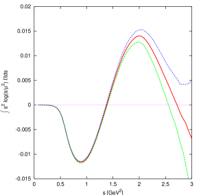
Figure 6.3: The integral over the spectral function needed for $\mbox{Im }G_{E}$.

at $\mu_{R}$ = 2 GeV and using for each distribution its second duality point $s_{0}$. Notice the much smaller error of ${\cal A}_{LR}$ and ${\cal A}^{\rm Lower}_{LR}$ when compared with $M_{2}$ and $M_{3}$. These values are all taken at the second duality point $s_{0}$ where the second WSR is satisfied. We plot ${\cal A}_{LR}$ as a function of $s_{0}$ in Fig. 6.3. The OPAL data give instead

$${\cal A}_{LR}(\mu_{R}) = (4.4_{-0.3}^{+0.4})\cdot 10^{-3}~{}{\rm GeV}^{6}\,;$$

$${\cal A}^{\rm Lower}_{LR}(\mu_{R}) = (3.8_{-0.5}^{+0.4})\cdot 10^{-3}~{}{\rm GeV}^{6}\,;$$

$${\cal A}^{\rm Higher}_{LR}(\mu_{R}) = (0.6_{-0.6}^{+0.8})\cdot 10^{-3}~{}{\rm GeV}^{6}$$

As a test, we can also calculate the electromagnetic pion mass difference in the chiral limit [153],

$${\cal B}_{LR} = {\displaystyle\int^{s_{0}}_{0}}\,{\rm d}t\,t\,\ln\left(\frac{t}{\mu_{R}^{2}}\right)\,\frac{1}{\pi}\,\mbox{Im }\,\Pi_{LR}^{T}(t)=\frac{4\pi F_{0}^{2}}{3\alpha_{QED}}\,\left(m_{\pi^{0}}^{2}-m_{\pi^{+}}^{2}\right)$$ (6.61)

$$= -(5.2\pm 0.5)\cdot 10^{-3}~{}{\rm GeV}^{4}~{}\mbox{(ALEPH)}\,;$$

$$= -(5.2\pm 0.6)\cdot 10^{-3}~{}{\rm GeV}^{4}~{}\mbox{(OPAL)}\,;$$

where we also used the value of $s_{0}$ given by the 2nd WSR. Notice that ${\cal B}_{LR}$ does not depend on $\mu_{R}$ due to the second WSR (6.4). The experimental number is

$$\frac{4\pi F_{0}^{2}}{3\alpha_{QED}}\,\left(m_{\pi^{0}}^{2}-m_{\pi^{+}}^{2}\right)_{\rm E.M.} = -(5.15\pm 0.90)\cdot 10^{-3}\,{\rm GeV}^{4}\,.$$ (6.62)

where we used $F_{0}=(87\pm 6)$ MeV as the chiral limit value of the pion decay constant and removed the QCD contributions [127].

For comparison we quote the central values using as $s_{0}$ the second duality point where the first WSR is satisfied

$$\begin{array}[]{rclrcl}s_{0}&=&(2.56^{+0.15}_{-0.14})~{}\mbox{GeV}^{2}\,,&{\cal A}_{LR}(2{\rm GeV})&=&(4.0_{-0.7}^{+0.6})\cdot 10^{-3}\,{\rm GeV}^{6}\,,\\ M_{2}&=&-(0.1_{-2.8}^{+3.0})\cdot 10^{-3}\,{\rm GeV}^{6},&{\cal A}^{Lower}_{LR}(2{\rm GeV})&=&(2.2\pm 2.1)\cdot 10^{-3}\,{\rm GeV}^{6},\\ M_{3}&=&(11_{-7}^{+9})\cdot 10^{-3}\,{\rm GeV}^{8}\,,&{\cal A}^{Higher}_{LR}(2{\rm GeV})&=&(1.8_{-1.6}^{+0.5})\cdot 10^{-3}\,{\rm GeV}^{6}.\end{array}$$ (6.66)

for ALEPH and for OPAL

$$\begin{array}[]{rclrcl}s_{0}&=&(2.53^{+0.17}_{-0.12})~{}\mbox{GeV}^{2}\,,&{\cal A}_{LR}(2{\rm GeV})&=&(3.4_{-0.8}^{+0.7})\cdot 10^{-3}\,{\rm GeV}^{6}\,,\\ M_{2}&=&(0.1_{-2.3}^{+2.8})\cdot 10^{-3}\,{\rm GeV}^{6},&{\cal A}^{Lower}_{LR}(2{\rm GeV})&=&(1.7^{+1.4}_{-1.3})\cdot 10^{-3}\,{\rm GeV}^{6},\\ M_{3}&=&(10_{-6}^{+9})\cdot 10^{-3}\,{\rm GeV}^{8}\,,&{\cal A}^{Higher}_{LR}(2{\rm GeV})&=&(1.7_{-1.3}^{+1.8})\cdot 10^{-3}\,{\rm GeV}^{6}.\end{array}$$ (6.70)

The errors are larger here. The value of $s_{0}$ where the first WSR is satisfied varies more and is somewhat larger than the $s_{0}$ where the second WSR is satisfied, this makes the last results more dependent on the spectral function at high $t$ which have large errors.

If one tried to see the results using the first duality point, where less duality with QCD is expected, we get that using the one from the 2nd WSR

$$\begin{array}[]{rclrcl}s_{0}&=&(1.47\pm 0.02)\,{\rm GeV}^{2}\;,&{\cal A}_{LR}(2{\rm GeV})&=&(3.3\pm 0.1)\cdot 10^{-3}\,{\rm GeV}^{6},\\ M_{2}&=&-(6.6\pm 0.2)\cdot 10^{-3}\,{\rm GeV}^{6},&{\cal A}^{Lower}_{LR}(2{\rm GeV})&=&(5.9\pm 0.2)\cdot 10^{-3}\,{\rm GeV}^{6},\\ M_{3}&=&-(12_{-2}^{+1})\cdot 10^{-3}\,{\rm GeV}^{8},&{\cal A}^{Higher}_{LR}(2{\rm GeV})&=&-(2.6\pm 0.1)\,{\rm GeV}^{6}.\end{array}$$ (6.74)

Notice that $M_{2}$ is not compatible with (6.4) with the central values differing by more than twice the error. The moment $M_{3}$ changes even sign with respect to the second duality point showing the problems of local duality violations for larger moments more dramatically. As argued before one should take the largest value of $s_{0}$ to ensure better local duality. However, the physical relevant moment ${\cal A}_{LR}$ is much more stable with $s_{0}$.

6.5 The Scalar–Pseudo-Scalar Two-Point Function   $\,\Pi_{SS+PP}^{(0-3)}(Q^{2})\,$

In this section we discuss some of the knowledge of the spectral function $\mbox{Im }\Pi_{SS+PP}^{(0-3)}(t)$ which governs the connected contribution to the matrix element of $Q_{8}$. In the large $N_{c}$ limit there is no difference between the singlet and triplet channel so the integral in (6.75) is $1/N_{c}$ suppressed and its contribution to $\mbox{Im }G_{E}$ is NNLO. But in the scalar-pseudo-scalar sector, violations of the large $N_{c}$ behaviour can be larger than in the vector-axial-vector channel. It is therefore interesting to determine the size of this contribution as well.

After adding the short-distance part to the long-distance part, the relevant integral is (6.40)

$$\,\frac{1}{48\pi^{2}}\frac{1}{\langle 0|\bar{q}q|0\rangle^{2}(\mu_{C})}\,\int_{0}^{\tilde{s}_{0}}{\rm d}t\,t\,\ln\left(\frac{t}{\mu^{2}}\right)\,\frac{1}{\pi}\,\mbox{Im }\Pi_{SS+PP}^{(0-3)}(t)\,,$$ (6.75)

This is the contribution of the connected part relative to the disconnected one. $\tilde{s}_{0}$ is the scale where in this channel QCD duality sets in. The scale $\mu$ is the cut-off scale. The dependence on this scale being NNLO in $1/N_{c}$ cannot match the present NLO order Wilson coefficients.

We can use models like the ones in [177] to evaluate the scalar part of the integrals. We only use the model there using the KLM [182] analysis, since only it ratifies (6.32) at a reasonable value of $\tilde{s}_{0}$ and, in addition, produce values for $L_{4}$, $L_{6}$ and $L_{8}$ compatible with phenomenology. In Fig. 6.4 we plotted for that parameterization the sum rule and the relative correction from the scalar part to the disconnected contribution $3\langle 0|\overline{q}q|0\rangle^{2}(\mu_{R})$ for $\mu=\mu_{R}=2$ GeV.

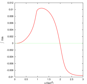
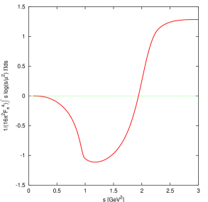
Figure 6.4: The sum rule (6.32) as a function of $\tilde{s}_{0}$ for the scalar part and the relative correction to the disconnected contribution for $Q_{8}$ using the same parametrization as a function of $\tilde{s}_{0}$ for $\mu_{R}=\mu=$ 2 GeV. Notice that the correction is small in the region where the sum rule is satisfied.

The value of the scalar part of Eq. (6.75) is about 0.18 at $\tilde{s}_{0}=(1.41$ GeV)².

In the large $N_{c}$ limit, a sensible alternative estimate is to use meson pole dominance. In the pseudo-scalar sector, the U(3)$\times$U(3) symmetry is broken by the chiral anomaly splitting the singlet $\eta_{1}$ mass away from the zero mass for the Goldstone boson octet.

Three meson intermediate states are not studied enough to be included at this level, we include instead the first $\pi^{\prime}$ resonance. This means including a massless Goldstone boson plus the first $\pi^{\prime}$ resonance and the singlet $\eta_{1}$. The pseudo-scalar sum rule in (6.32) requires the following relation between the octet and the singlet couplings to the pseudo-scalar current for $\tilde{s}_{0}\simeq 2.0$ GeV²,

$$F_{0}^{2}+F_{\pi^{\prime}}^{2}=F_{\eta_{1}}^{2}\,.$$ (6.76)

Phenomenologically $F_{\pi^{\prime}}^{2}/F_{0}^{2}<<1$ [183] and $F_{0}\simeq F_{\eta_{1}}$.

We can introduce a scalar meson octet $S_{8}$ and a singlet $S_{1}$ using the methods of [37]. The coupling constant for the octet can be denoted by $c_{m}$ and has been estimated in [37, 148] to be about $(43\pm 14)$ MeV. In fact, the sum rule (6.30) is a property of QCD and relates in this approximation $c_{m}$ to $F_{0}$

$$c_{m}^{2}=\frac{1}{8}\left[F_{0}^{2}+F_{\pi^{\prime}}^{2}+\cdots\right]=\frac{F_{\eta_{1}}^{2}}{8}\simeq\frac{F_{0}^{2}}{8}$$ (6.77)

which numerically agrees quite well with the phenomenological estimate.

The scalar sum rule in (6.32) requires the singlet and the octet components to have the same coupling leading to a relative correction from the scalar integral to the disconnected contribution of

$$\frac{1}{12\pi^{2}}\frac{F_{\eta_{1}}^{2}}{F_{0}^{4}}\,\left[M_{S_{1}}^{2}\ln\left(\frac{M_{S_{1}}}{\mu}\right)-M_{S_{8}}^{2}\ln\left(\frac{M_{S_{8}}}{\mu}\right)\right].$$ (6.78)

using both sum rules and the lowest meson dominance approximation.

The contribution from the pseudo-scalar connected two-point function relative the disconnected contribution can then be evaluated to

$$\frac{1}{12\pi^{2}}\frac{F_{\eta_{1}}^{2}}{F_{0}^{4}}\,\left[M_{\eta_{1}}^{2}\,\ln\left(\frac{M_{\eta_{1}}}{\mu}\right)\,-\frac{F_{\pi^{\prime}}^{2}}{F_{\eta_{1}}^{2}}\,M_{\pi^{\prime}}^{2}\ln\left(\frac{M_{\pi^{\prime}}}{\mu}\right)\right]\,.$$ (6.79)

The contribution of the $\pi^{\prime}$ is negligible. Using a Breit-Wigner shape for the $\pi^{\prime}$ contribution do not change much the result due to the small coupling of the $\pi^{\prime}$.

As said before the scale $\mu$ is free and cannot be at present matched with OPE QCD since it is a NNLO order in $1/N_{c}$ effect. The scale independence is reached when the sum rule

$$\tilde{M}_{1} = M_{S_{8}}^{2}-M_{S_{1}}^{2}-M_{\eta_{1}}^{2}+\frac{F_{\pi^{\prime}}^{2}}{F_{\eta_{1}}^{2}}M_{\pi^{\prime}}^{2}=0$$ (6.80)

which is $O(N_{c}^{2}\alpha^{2})$ (6.2.2) is fulfilled. This sum rule is very well satisfied in the linear $\sigma$ model, see e.g. [177].

The masses $M_{\eta_{1}}\simeq 0.86$ GeV (chiral limit value) $M_{\pi^{\prime}}\simeq 1.3$ GeV are known. The masses of the singlet and octet of scalars are not so well known. Using $M_{S_{1}}=M_{\sigma}\simeq 0.5$ GeV and $M_{S_{8}}=M_{a_{0}(980)}\simeq 0.98$ GeV the correction to the disconnected contribution is almost independent of the scale $\mu$, neglecting the $\pi^{\prime}$ and is independent of $\mu$ for $F_{\pi^{\prime}}^{2}/F_{0}^{2}=0.017$.

The scalar form factor in [177] is obtained from data and dispersion relations up to 1 GeV and Breit-Wigner shapes above. The result of using these models agreed with the results of naive narrow widths for the lowest scalar resonances. These were constructed to fulfill the short-distance QCD constraints and also produces reasonable values for $L_{6}$ and $L_{8}$. Here, we have also tried Breit-Wigner shapes for the scalar mesons instead of narrow widths and again find results in the same ball park. Now, we also have used the scalar form factors obtained in [184] where the lowest scalar triplet and singlet resonances are generated dynamically for energies up to 1 GeV and Breit-Wigner shapes above and we get similar results.

In all the estimates, we got negative corrections to the disconnected part in the region between -10% to -30%. Though the connected scalar-pseudoscalar contribution in (6.75) cannot be used at a quantitative level at present, the results above indicate that is difficult to have corrections larger than $\pm$30% to the disconnected part.

Of course, the scale dependence left in (6.75) is unsatisfactory in principle but small since the sum rule (6.80) is quite well satisfied.

6.6 Numerical Results for the Matrix-Elements and Bag Parameters

The vacuum expectation value in the chiral limit of $Q_{7}$ itself is related directly to $B_{7\chi}$. This allows us to obtain

$$\langle 0|O_{6}^{(1)}(0)|0\rangle^{NDR}(\mu_{R}) = -\left(1+\frac{1}{24}a(\mu_{R})\right)\,\frac{3}{32\pi^{2}}{\cal A}_{LR}(\mu_{R})$$ (6.81)

$$+ \frac{1}{48}\,a(\mu_{R})\,\left[3\langle 0|\overline{q}q|0\rangle^{2}(\mu_{R})+\frac{1}{16\pi^{2}}{\cal A}_{SP}(\mu_{R},\mu_{C})\right]\,;$$

$$\langle 0|O_{6}^{(1)}(0)|0\rangle^{HV}(\mu_{R}) = -\left(1-\frac{11}{24}a(\mu_{R})\right)\frac{3}{32\pi^{2}}\,{\cal A}_{LR}(\mu_{R})$$ (6.82)

$$- \frac{11}{48}\,a(\mu_{R})\,\left[3\langle 0|\overline{q}q|0\rangle^{2}(\mu_{R})\,+\frac{1}{16\pi^{2}}{\cal A}_{SP}(\mu_{R},\mu_{C})\right]\,.$$

For the numerics, we use the value of the condensate obtained in the $\overline{MS}$ scheme in [130],

$$\langle 0|\overline{q}q|0\rangle(2{\rm GeV}) = -(0.018\pm 0.004)\,{\rm GeV}^{3}\,,$$ (6.83)

the numerical results of Eq. (6.4),

$$a(2~{}GeV)=0.102$$ (6.84)

and neglect, in first approximation, the integral over the scalar–pseudo-scalar two-point function.

The weighted average of the first and second WSR results for ${\cal A}_{LR}(2{\rm GeV})$ from ALEPH data is

$${\cal A}^{\rm ALEPH}_{LR}(2{\rm GeV})=(4.5\pm 0.5)\cdot 10^{-3}~{}{\rm GeV}^{6}$$ (6.85)

and from OPAL data

$${\cal A}^{\rm OPAL}_{LR}(2{\rm GeV})=(4.2\pm 0.4)\cdot 10^{-3}~{}{\rm GeV}^{6}\,.$$ (6.86)

Though the systematic errors aver very correlated, since the central values are very similar we take the simple average of both results as our result

$${\cal A}_{LR}(2{\rm GeV})=(4.35\pm 0.50)\cdot 10^{-3}~{}{\rm GeV}^{6}\,$$ (6.87)

and obtain

$$\langle 0|O_{6}^{(1)}(0)|0\rangle^{NDR}(2{\rm GeV})=-(4.0\pm 0.5)\cdot 10^{-5}~{}{\rm GeV}^{6}$$ (6.88)

$$= \left(-(4.2\pm 0.5)+(0.2\pm 0.1)\right)\cdot 10^{-5}~{}{\rm GeV}^{6}$$

$$= \left((-3.3\pm 0.5)+(-0.9\pm 0.8)+(0.2\pm 0.1)\right)\cdot 10^{-5}~{}{\rm GeV}^{6}$$

and

$$\langle 0|O_{6}^{(1)}(0)|0\rangle^{HV}(2{\rm GeV})=-(6.2\pm 1.0)\cdot 10^{-5}~{}{\rm GeV}^{6}$$ (6.89)

$$= \left((-3.9\pm 0.5)-(2.3\pm 0.9)\right)\cdot 10^{-5}~{}{\rm GeV}^{6}$$

$$= \left((-3.1\pm 0.5)+(-0.8\pm 0.7)-(2.3\pm 0.9)\right)\cdot 10^{-5}~{}{\rm GeV}^{6}$$

where we quote, namely, the total result, the integral and the vacuum expectation value separately and in the last case also the long and short-distance part of the integral separately.

The short-distance part of the integral, the second term in the above, is the contribution of all higher dimensional operators. We find that its contribution is between a few % up to 35 % depending on the value of $\mu$. At $\mu=2$ GeV it is somewhat larger than the error on the integral cut-off at $\mu$.

Similarly, the matrix-element of $Q_{8}$ is directly related to $B_{8}$ and we obtain

$$\langle 0|O_{6}^{(2)}(0)|0\rangle^{NDR}(2{\rm GeV}) = \left[1+\frac{23}{12}\,a(2{\rm GeV})\right]\times$$ (6.90)

$$\times\left[3\,\langle 0|\overline{q}q|0\rangle^{2}(2{\rm GeV})+\frac{1}{16\pi^{2}}{\cal A}_{SP}(2\rm{GeV},2\rm{GeV})\right]\,$$

$$- \frac{27}{64\pi^{2}}\,a(2{\rm GeV})\,{\cal A}_{LR}(2{\rm GeV})\,.$$

$$\langle 0|O_{6}^{(2)}(0)|0\rangle^{HV}(2{\rm GeV}) = \left[1+\frac{35}{12}\,a(2{\rm GeV})\right]\times$$ (6.91)

$$\times\left[3\,\langle 0|\overline{q}q|0\rangle^{2}(2{\rm GeV})+\frac{1}{16\pi^{2}}{\cal A}_{SP}(2\rm{GeV},2\rm{GeV})\right]\,$$

$$+ \frac{9}{64\pi^{2}}\,a(2{\rm GeV})\,{\cal A}_{LR}(2{\rm GeV})\,.$$

Using the same input as above we obtain

$$\langle 0|O_{6}^{(2)}(0)|0\rangle^{NDR}(2{\rm GeV}) = (1.2\pm 0.5)\cdot 10^{-3}\,{\rm GeV}^{6}\,,$$

$$\langle 0|O_{6}^{(2)}(0)|0\rangle^{HV}(2{\rm GeV}) = (1.3\pm 0.6)\cdot 10^{-3}\,{\rm GeV}^{6}\,,$$ (6.92)

where the contribution of the integral over $\mbox{Im }\Pi_{LR}^{T}$ is at the 1% level and thus totally negligible.

Another combination of these two matrix-elements can also be obtained from an integral over the ALEPH data[65, 69] by putting (6.2.1) and (6.18) in (6.4) including also the $\alpha_{S}$ correction of the appendix :

$$M_{2} = \int_{0}^{s_{0}}{\rm d}t\,t^{2}\,\frac{1}{\pi}\,\mbox{Im }\Pi_{LR}^{T}(t)={\displaystyle\sum_{i=1}}\,C^{(i)}_{6}(s_{0},s_{0})\,O^{(i)}_{6}(s_{0})$$ (6.93)

$$= -\frac{4\pi^{2}}{3}\,a(s_{0})\left[2\left(1+\frac{13}{8}\,a(s_{0})\right)\,\langle 0|O_{6}^{(1)}(0)|0\rangle^{NDR}(s_{0})\right.$$

$$+ \left.\,\left(1+\frac{25}{8}a(s_{0})\right)\,\langle 0|O_{6}^{(2)}(0)|0\rangle^{NDR}(s_{0})\right]\,$$

$$= -\frac{4\pi^{2}}{3}\,a(s_{0})\left[2\left(1+\frac{41}{8}\,a(s_{0})\right)\,\langle 0|O_{6}^{(1)}(0)|0\rangle^{HV}(s_{0})\right.$$

$$+ \left.\,\left(1+\frac{21}{8}a(s_{0})\right)\,\langle 0|O_{6}^{(2)}(0)|0\rangle^{HV}(s_{0})\right]\,.$$

$$= -4\pi^{2}a(s_{0})\left[\left(1+\frac{61}{12}a(s_{0})\right)\,\left[\langle 0|\overline{q}q|0\rangle^{2}(s_{0})+\frac{1}{48\pi^{2}}{\cal A}_{SP}(s_{0},s_{0})\right]\,\right.$$

$$- \left.\left(1+\frac{47}{12}a(s_{0})\right)\frac{1}{16\pi^{2}}{\cal A}_{LR}(s_{0})\right]$$

The right hand-side is physical and we checked that is independent of the scale $s_{0}$ and scheme. We can therefore evaluate it at $s_{0}=4$ GeV². The contribution from $\langle 0|O_{6}^{(1)}(0)|0\rangle^{NDR}$ $(s_{0})$ is numerically very small and we obtain

$$M_{2}=-(2.0\pm 0.9)\cdot 10^{-3}~{}\mbox{GeV}^{6}\,,$$ (6.94)

perfectly compatible within errors both with the result obtained from the data in Eq. (6.4) and with the result (6.4). This confirms our results on the size of the integral over $\mbox{Im }\Pi_{SS+PP}(t)$, which can therefore be considered negligible within the present accuracy of the disconnected contribution and $M_{2}$.

There is another sum rule which combines the two matrix elements,

$$\tilde{M}_{1} = \int_{0}^{\tilde{s}_{0}}{\rm d}t\,t\,\frac{1}{\pi}\,\mbox{Im }\Pi_{SS+PP}(t)=-{\displaystyle\sum_{i=1}}\,\tilde{C}^{(i)}_{6}(s_{0},s_{0})\,O^{(i)}_{6}(s_{0})$$

$$= -\frac{\pi^{2}}{4}\,a(s_{0})^{2}\,\left[211\,\langle 0|O_{6}^{(2)}(0)|0\rangle(\tilde{s}_{0})+90\,\langle 0|O_{6}^{(1)}(0)|0\rangle(\tilde{s}_{0})\right]+O(a^{3})\,.$$

For the calculation of the coefficients see Appendix A.2. This sum rule is much less accurate than $M_{2}$ since the leading terms are $\alpha_{S}^{2}$ and the value of $\tilde{M}_{1}$ is not known directly either. Therefore we don’t use it.

The numerical estimates of the disconnected part, ${\cal A}_{SP}$, given above change these numbers somewhat but within the errors quoted.

These results can also be expressed in terms of the bag parameters:

$$B_{7\chi}^{NDR}(2{\rm GeV}) = 0.75\pm 0.20\;;\quad B_{7\chi}^{HV}(2{\rm GeV})=1.15\pm 0.30\;$$

$$B_{8\chi}^{NDR}(2{\rm GeV}) = 1.2\pm 0.3\;;\quad B_{8\chi}^{HV}(2{\rm GeV})=1.3\pm 0.4\,.$$ (6.96)

We can also express it in terms of $\mbox{Im }G_{E}$:

$$F_{0}^{6}~{}\mbox{Im }G_{E} = \mbox{Im }\tau(-2.1\pm 0.9)~{}10^{-6}~{}\mbox{GeV}^{6}\,$$ (6.97)

which is quite compatible with the estimate in [72].

6.7 Comparison with earlier results

To compare with other results in the literature we propose to use the VEVs $\langle 0|O_{6}^{(1)}|0\rangle$ and $\langle 0|O_{6}^{(2)}|0\rangle$. The reason is that these quantities are what [80, 81, 82] and we directly compute. The matrix elements of $K\to\pi\pi$ through $Q_{7}$ and $Q_{8}$, in the chiral limit, can be expressed as follows [72]

$$M_{2}[Q_{7}](\mu_{R}) = \langle(\pi\pi)_{I=2}|Q_{7}|K^{0}\rangle(\mu_{R})=-\sqrt{\frac{2}{3}}\,\frac{\langle 0|\overline{q}q|0\rangle^{2}(\mu_{C})}{F_{0}^{3}}\,\,B_{7\chi}(\mu_{C},\mu_{R})\,$$

$$= 2\sqrt{6}\,\frac{\langle 0|O_{6}^{(1)}|0\rangle_{\chi}(\mu_{R})}{F_{0}^{3}}\,;$$

$$M_{2}[Q_{8}](\mu_{R}) = \langle(\pi\pi)_{I=2}|Q_{8}|K^{0}\rangle(\mu_{R})=-\sqrt{6}\,\frac{\langle 0|\overline{q}q|0\rangle^{2}(\mu_{C})}{F_{0}^{3}}\,\,B_{8\chi}(\mu_{C},\mu_{R})\,$$ (6.98)

$$= -\frac{\sqrt{6}}{3}\,\frac{\langle 0|O_{6}^{(2)}|0\rangle_{\chi}(\mu_{R})}{F_{0}^{3}}\,.$$

The different results obtained in the literature using analytical and lattice methods for the matrix elements in the NDR scheme and at $\mu=2\mbox{\rm GeV}$ are collected in Tables 6.1 and 6.2

Reference	$-6\times 10^{4}\langle 0|O_{6}^{(1)}|0\rangle^{NDR}_{\chi}\,{\rm GeV}^{-6}$
$B_{7}^{\chi}$(2 GeV)=$B_{8}^{\chi}$(2 GeV)=1	$3.2\pm 1.3$
This work, [9] (SS+PP=0)	$2.4\pm 0.3$
This work, [9] (Data & Duality FESR)	$2.4\pm 0.3$
Cirigliano et al., [85] (Data & Fitted FESR)	$2.2\pm 0.5$
Knecht et al., [82] $N_{c}\to\infty$,MHA	$1.1\pm 0.3$
Narison, [81] Data & Tau-like FESR	$2.1\pm 0.6$
CP-PACS Coll., [86] lattice(chiral)	$2.4\pm 0.3$ (stat.)
RBC Coll., [87] lattice(chiral)	$2.8\pm 0.4$ (stat.)
${\rm SPQ_{CD}R}$ Coll., [89] lattice(Wilson)	$1.4\pm 0.1$ (stat.)

Table 6.1: The values of the VEV $\langle 0|O_{6}^{(1)}|0\rangle_{\chi}$ in the NDR scheme at $\mu_{R}=2$ GeV.

Reference	$10^{3}\langle 0|O_{6}^{(2)}|0\rangle^{NDR}_{\chi}\,{\rm GeV}^{-6}$
$B_{7}^{\chi}$(2 GeV)=$B_{8}^{\chi}$(2 GeV)=1	$1.0\pm 0.4$
This work, [9] (SS+PP=0)	$1.2\pm 0.5$
This work, [9] (Data & Duality FESR)	$1.2\pm 0.7$
Cirigliano et al., [85] (Data & Fitted FESR)	$1.5\pm 0.3$
Knecht et al., [82] $N_{c}\to\infty$,MHA	$2.3\pm 0.7$
Narison, [81] Data & Tau-like FESR	$1.4\pm 0.4$
CP-PACS Coll., [86] lattice(chiral)	$1.0\pm 0.2$ (stat.)
RBC Coll., [87] lattice(chiral)	$1.1\pm 0.2$ (stat.)
${\rm SPQ_{CD}R}$ Coll., [89] lattice(Wilson)	$0.8\pm 0.1$ (stat.)

Table 6.2: The values of the VEV $\langle 0|O_{6}^{(2)}|0\rangle_{\chi}$ in the NDR scheme at $\mu_{R}=2$ GeV.

Within the present accuracy of $\langle 0|\bar{q}q|0\rangle$, the disconnected contribution ${\cal A}_{SP}$ in (6.2.3) –second line in the tables– is perfectly compatible with our full result –third line in the tables–, so that we cannot conclude a large deviation from the large $N_{C}$ result within the present accuracy. Notice that we include in this result- third line in Table 6.2- ${\cal O}(\alpha_{S})$ corrections that are indeed leading order in $1/N_{C}$ (see (6.90)) which are usually disregarded in the factorization approaches, this makes the chiral limit $B_{8}^{\chi}(2GeV)$ parameter larger than one by around 20% to 30%.

We agree with the analytical results in [81, 85]. We are borderline within errors with the value of $\langle 0|O_{6}^{(2)}|0\rangle^{NDR}_{\chi}$ in [82] though their central value is twice ours, but our results for $\langle 0|O_{6}^{(1)}|0\rangle^{NDR}_{\chi}$ are not compatible.

The agreement between our results and the lattice results is quite good in the case of the chiral fermion determinations but not so good in the results coming from calculations using Wilson fermions. The lattice determinations are made in the quenched approximation and the quoted errors -which are much smaller than ours for $\langle 0|O_{6}^{(2)}|0\rangle^{NDR}_{\chi}$- are only statistical ones. The present lattice results are larger than the earlier estimates and the value of $\langle 0|O_{6}^{(2)}|0\rangle^{NDR}_{\chi}$ in [85] is smaller than their previous result in [83]. This makes possible the agreement with our results.

We have not quoted the results from the lattice calculation using staggered fermions in [88], since they give their results in terms of the bag parameters. In the chiral limit, the values they obtained for the bag parameters in the NDR scheme are [185] $B_{7}^{\chi}(2\mbox{\rm GeV})=0.85\pm 0.04$ and $B_{8}^{\chi}(2\mbox{\rm GeV})=0.89\pm 0.05$.

6.7.1 Rôle of Higher Dimensional Operators

We clarified here the role of the higher than six dimensional operators, an issue raised in [169]. In our scheme they remove the $\mu$-dependence which is not covered by the renormalization group. The role of these operators was analyzed in [9] and later in [85]

The effect of higher dimension operators in our approach is to add ${\cal A}_{LR}^{\rm Higher}(\mu)$ to the low energy contribution ${\cal A}_{LR}^{\rm Lower}(\mu)$, these are defined in Eq. (6.4),

$${\cal A}_{LR}(\mu) = {\cal A}_{LR}^{\rm Higher}+{\cal A}_{LR}^{\rm Lower}=\int_{0}^{s_{0}}{\rm d}t\,t^{2}\,\ln\left(\frac{t}{\mu^{2}}\right)\,\frac{1}{\pi}\,\mbox{Im }\Pi_{LR}^{T}(t)\,$$ (6.99)

where $\mu$ is an Euclidean cut-off. It is clear than the contribution of higher than dimension six operators is less important only for values of $\mu^{2}$ larger than $s_{0}$, where $\mbox{Im }\Pi^{T}_{LR}$ vanishes because of local duality. In Figure 6.5 we plot the two separate contributions and the sum as a function of $\mu$.

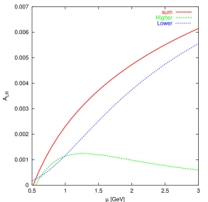
Figure 6.5: The separate contributions to ${\cal A}_{LR}$ and the sum. “Higher” labels the effect of the higher than six dimensional operators in the short-distance contribution and “Lower” the long-distance part.

From the figure we can see for $\mu$ larger than 2 GeV the contribution of all higher dimensional operators is less than 25 %. We agree with [169] that for the matrix elements that involve integrals of $\mbox{Im }\Pi^{T}_{LR}$ one has to go to such values of $\mu$ to disregard the contribution of higher dimensional operators. The contribution we find is somewhat smaller than in [169] since we include the effect of all higher order operators, not just dimension eight.

The high value of $\mu$ is set by the threshold of perturbative QCD $s_{0}$ which depends very much on the spectral function and on the integrand behaviour. In fact, from [151] one can see that relevant spectral function for the 27-plet coupling reaches the perturbative QCD behaviour very soon, from 0.7 GeV to 1 GeV. The OPE matched impressively well with the hadronic ansatz at such low values with just dimension six operators. Therefore though higher dimensional operators appear one can expect smaller contributions in cases like $G_{27}$ and $\mbox{Re }G_{8}$.

The matrix-elements studied in this paper might be special in the sense that they follow from integrals over spectral functions which have no contributions at short-distances from the unit operator or the dimension four operators. As the good matching at low scales in the example in [151] shows, the other quantities which have these contributions might have much smaller higher dimension effects.

Chapter 7 Application to $\varepsilon_{K}^{\prime}$

One of the applications of the hadronic model introduced in Chapter 5 is the calculation of $\mbox{Im }G_{8}$ using the $X$-boson method. This can be used to confirm the large value found in [72] and to study its origin analytically.

At a first step, we will discuss the update presented in [10] of the results of [72]. The new things we would like to input are the non-FSI corrections which after the work in [21, 64, 77, 78] are known. We also use the recent complete isospin breaking result of [70]. The result in [72] did contain the FSI corrections but not the non-FSI which were unknown at that time. The other new input is the $\Delta I=3/2$ contribution calculated in the chiral limit and at NLO in [9] and discussed in Chapter 6.

The chiral corrections to the LO in CHPT predictions for the ratios of amplitudes in (2.22)

$$\varepsilon_{K}^{\prime}\,\simeq\,\frac{i}{\sqrt{2}}\frac{\mbox{Re }a_{2}}{\mbox{Re }a_{0}}\left[\frac{\mbox{Im }a_{2}}{\mbox{Re }a_{2}}-\frac{\mbox{Im }a_{0}}{\mbox{Re }a_{0}}\right]e^{i(\delta_{2}-\delta_{0})}$$ (7.1)

are introduced in (2.36) and (2.40) through the factors $C_{0}$ and $C_{2}$

$$\frac{\mbox{Im }a_{0}}{\mbox{Re }a_{0}}=\left(\frac{\mbox{Im }a_{0}}{\mbox{Re }a_{0}}\right)^{LO}{\cal C}_{0}\,,\quad\frac{\mbox{Im }a_{2}}{\mbox{Re }a_{2}}=\left(\frac{\mbox{Im }a_{2}}{\mbox{Re }a_{2}}\right)^{LO}{\cal C}_{2}+\Omega_{{\rm eff}}\frac{\mbox{Im }a_{0}}{\mbox{Re }a_{0}}\,.$$ (7.2)

The parameter $\Omega_{eff}$ includes the effects of isospin breaking -see Section 2.4.1.

In the ratio $\mbox{Re }a_{0}/\mbox{Re }a_{2}$ the chiral corrections can be also introduced by a multiplicative factor $C_{\Delta I=1/2}$ as follows

$$\frac{\mbox{Re }a_{0}}{\mbox{Re }a_{2}}=\left(\frac{\mbox{Re }a_{0}}{\mbox{Re }a_{2}}\right)^{LO}{\cal C}_{\Delta I=1/2}\,.$$ (7.3)

We get from the fit to experimental $K\to\pi\pi$ amplitudes in [64]

$$C_{\Delta I=1/2}=\frac{{\cal S}_{0}}{{\cal S}_{2}}=\frac{1.90\pm 0.16}{1.56\pm 0.19}=1.22\pm 0.15\,\,\,$$ (7.4)

Where ${\cal S}_{\rm I}$ are the chiral corrections to $\mbox{Re }a_{I}$ to all orders while we call $\cal{T}_{\rm I}$ to the chiral corrections to $\mbox{Im }a_{I}$ to all orders. Therefore, they contain the FSI corrections which were exhaustively studied in [21] plus the non-FSI corrections which are a sizable effect and of opposite direction. All these chiral corrections contain the large overall known factor $f_{K}f_{\pi}^{2}/F_{0}^{3}\simeq 1.47$ from wave function renormalization.

The imaginary parts $\mbox{Im }a_{I}$ get FSI corrections identical to $\mbox{Re }a_{I}$ owing to Watson’s theorem. In addition, both due to octet dominance in $\mbox{Re }a_{0}$ and $\mbox{Im }a_{0}$ and to the numerical dominance of the non-analytic terms at NLO in $K\to\pi\pi$ amplitudes [21, 64, 77]

$$C_{0}=\,{{\cal T}_{0}}/{{\cal S}_{0}}\,\simeq 1.0\pm 0.2\,,$$ (7.5)

to a good approximation.

The situation is quite different for $\mbox{Im }a_{2}$ which is proportional to $\mbox{Im }(e^{2}G_{E})$ at lowest order since $\mbox{Im }G_{27}=0$ in the Standard Model. From the works [21, 64, 78] we also know that

$$C_{2} = \frac{{\cal T}_{2}}{{\cal S}_{2}}\simeq\frac{0.70\pm 0.21-0.73L_{4}/10^{-3}}{1.56\pm 0.18}$$ (7.6)

$$= 0.45\pm 0.15-0.47\frac{L_{4}}{10^{-3}}\,.$$

At LO in CHPT, the result is obtained by substituting directly in (2.22) the value of the ratios given in (3.3) [10]

$$\left(\frac{\varepsilon^{\prime}_{K}}{\varepsilon_{K}}\right)^{LO} = ((-10.8\pm 5.4)+(2.7\pm 0.8))\,\mbox{Im }\tau\,$$ (7.7)

$$= -(8.1\pm 5.5)\,\mbox{Im }\tau=(4.9\pm 3.3)\times 10^{-3}\,.$$

This result is scheme independent and very stable against the short-distance scale as can be seen in Figure 7.1.

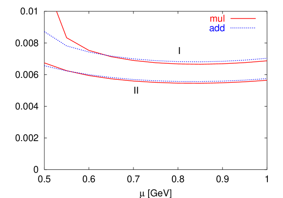
Figure 7.1: Matching of the short-distance scale dependence of our LO in CHPT $\varepsilon^{\prime}_{K}/\varepsilon_{K}$ prediction. Labels I and II are for two different values of $\alpha_{S}$. The two curves for two choices of perturbative matching, see [72]. Notice the quality of the matching.

The difference with the result in Figure 7.1 [72] is due to the new values of $\mbox{Im }\tau$ in (3.38) and $\mbox{Re }G_{8}$ and $G_{27}$ in (3.35).

Including the known and estimated higher order CHPT corrections, we get [10]

$$-\frac{1}{|\varepsilon_{K}|\sqrt{2}}\,\frac{\mbox{Re }a_{2}}{\mbox{Re }a_{0}}\,\frac{\mbox{Im }a_{0}}{\mbox{Re }a_{0}}=-(8.9\pm 4.8)\,\mbox{Im }\tau\,$$ (7.8)

and

$$\frac{1}{|\varepsilon_{K}|\sqrt{2}}\,\frac{\mbox{Re }a_{2}}{\mbox{Re }a_{0}}\,\frac{\mbox{Im }a_{2}}{\mbox{Re }a_{2}}=((1.0\pm 0.3)+(0.5\pm 0.7))\,\mbox{Im }\tau\,=(1.5\pm 0.8)\,\mbox{Im }\tau\,.$$

where the second part comes from isospin breaking contribution with $\Omega_{eff}=0.06\pm 0.08$ [70], and we used $L_{4}=0$ in (7.6). And therefore,

$$\frac{\varepsilon^{\prime}_{K}}{\varepsilon_{K}} = ((-8.9\pm 4.8)+(1.5\pm 0.8))\,\mbox{Im }\tau\,$$ (7.9)

$$= -(7.4\pm 4.9)\,\mbox{Im }\tau=(4.5\pm 3.0)\times 10^{-3}$$

to be compared to the world average [61, 62]

$$\mbox{Re }\left(\frac{\varepsilon^{\prime}_{K}}{\varepsilon_{K}}\right){\Bigg{|}}_{\rm exp}=(1.66\pm 0.16)\times 10^{-3}\,.$$ (7.10)

Though the central value of our Standard Model prediction in (7.9) is a factor around 3 too large, within the big uncertainties it is still compatible with the experimental result. Two immediate consequences of the analysis above, namely, the LO CHPT prediction (7.7) is actually very close of the the final result (7.9) and second, the part with $\Delta I=1/2$ dominates when all higher order CHPT corrections are included.

The large final uncertainty we quote in (7.9) is mainly due to the uncertainties of (i) the chiral limit quark condensate, which is not smaller than 20%, (ii) $L_{5}$, which is around 30%, and (iii) the NLO in $1/N_{c}$ corrections to the matrix element of $Q_{6}$, which is around 20%. All of them together make the present prediction for the $\Delta I=1/2$ contribution to $\varepsilon^{\prime}_{K}$ to have an error around 55%. Reduction in the uncertainty of all these inputs, especially of the quark condensate and $L_{5}$ is needed to obtain a reasonable final uncertainty.

We substituted the value used in [72] for $\mbox{Im }(e^{2}G_{E})$ by the one in (3.39), notice however that numerically they coincide within errors. There are also large uncertainties in the $\Delta I=3/2$ component coming from isospin breaking [70], and more moderate in the non-FSI corrections to $\mbox{Im }a_{2}$, fortunately the impact of them in the final result is not as large as the ones associated to the $\Delta I=1/2$ component.

Assuming the $\Delta I=3/2$ component of $\varepsilon^{\prime}_{K}$ is fixed to be the one in (3.39) as indicated by the analytic methods [9, 81, 82, 85] and lattice [86, 87, 138, 139], one can try to extract the value of $\mbox{Im }G_{8}$ from the experimental result in (7.10). We get

$$\mbox{Im }G_{8}=(2.0^{+0.7}_{-0.4})\,\left(\frac{87{\rm MeV}}{F_{0}}\right)^{4}\,\mbox{Im }\tau$$ (7.11)

i.e. the central value coincides with the large $N_{c}$ result for $\mbox{Im }G_{8}$ within 30% of uncertainty. This value has to be compared to the result in [72] $\mbox{Im }G_{8}=(4.4\pm 2.2)\left(87{\rm MeV}/F_{0}\right)^{4}\,\mbox{Im }\tau$.

More work is needed to confirm the large value of $\mbox{Im }G_{8}$ obtained in [72]. We plan to analyze the origin of this value using the $X$-boson method as done in [72] but substituting the ENJL model by the hadronic model described in Chapter 5, that allow us to perform all calculations analytically. We intend to see the effect of the vector, axial-vector and scalar sources as well as the possible cancellations of their contributions. This will shed light on the leading large hadronic contributions which produce this $\mbox{Im }G_{8}$.

7.1 $\varepsilon_{K}^{\prime}$ with a Different Set of Input Parameters

Alternatively, we can calculate $\varepsilon_{K}^{\prime}$ using as input parameters the values of $\mbox{Re }G_{8}$ and $G_{27}$ obtained in the second reference in [70] where the leading isospin breaking effects are included. The values of the couplings found there, after normalizing them to $F_{0}=87\mbox{\rm MeV}$ -in [70] a lower value $F_{0}=85.7\mbox{\rm MeV}$ is used- are

$$\mbox{Re }G_{8}=\left(6.5\pm 0.26\right)\,\left(\frac{87{\rm MeV}}{F_{0}}\right)^{4}\,{\rm and}\,G_{27}=\left(0.54\pm 0.02\right)\,\left(\frac{87{\rm MeV}}{F_{0}}\right)^{4}\,.$$ (7.12)

Notice that the value of $G_{27}$ and $\mbox{Re }G_{8}$ in (7.12) are compatible with those in (3.35), but the central values are somewhat different. With these inputs, we get

$$-\frac{1}{|\varepsilon_{K}|\sqrt{2}}\,\frac{\mbox{Re }a_{2}}{\mbox{Re }a_{0}}\,\frac{\mbox{Im }a_{0}}{\mbox{Re }a_{0}}=-(10.8\pm 5.4)\,\mbox{Im }\tau\,$$ (7.13)

and

$$\frac{1}{|\varepsilon_{K}|\sqrt{2}}\,\frac{\mbox{Re }a_{2}}{\mbox{Re }a_{0}}\,\frac{\mbox{Im }a_{2}}{\mbox{Re }a_{2}}=((1.2\pm 0.3)+(0.6\pm 0.9))\,\mbox{Im }\tau\,=(1.8\pm 0.9)\,\mbox{Im }\tau\,.$$

where the second part, as in (7), comes from isospin breaking contribution with $\Omega_{eff}=0.06\pm 0.08$ [70].

The final value for the ratio $\varepsilon_{K}^{\prime}/\varepsilon_{K}$ from this set of input parameters is

$$\frac{\varepsilon^{\prime}_{K}}{\varepsilon_{K}} = ((-10.8\pm 5.4)+(1.8\pm 0.9))\,\mbox{Im }\tau\,$$ (7.14)

$$= -(8.9\pm 5.4)\,\mbox{Im }\tau=(5.4\pm 3.3)\times 10^{-3}$$

that is compatible with our result in (7.9). The difference between both results mainly comes from the different values of $\mbox{Re }G_{8}$ obtained by the fits to experimental data in [64] and [70].

Chapter 8 Conclusions

A. Charged Kaon $K\to 3\pi$ CP-Violating Asymmetries

We have performed the first full analysis at NLO in CHPT of the CP-violating asymmetries in the slope $g$ and the decay rate $\Gamma$ for the disintegration of charged Kaons into three pions. We have done the full order $p^{4}$ calculation for $K\to 3\pi$ and completely agree with the recent results in [64]. To give the CP-asymmetries at NLO, one needs the FSI phases at NLO also, i.e. at two loops. This is not available at present. We have calculated the dominant two-bubble contributions using the optical theorem and the known one-loop and tree level results in Appendix B.4 as explained in Section 4.4.1. Due to the small phase space available for the re-scattering effects of the final tree pions one expects the rest of the FSI to be very suppressed. We have included this contribution in our final numbers. As a byproduct, we have predicted the isospin I=2 FSI phase at NLO and two combinations of matrix elements of the isospin I=1 FSI re-scattering matrix $\mathbb{R}$ at NLO. They can be found numerically in Section 4.4.1 and analytically in Appendix B.4.5. We have given analytical expressions for all the results in the Appendices B.1, B.2, B.3, and B.4.

Our final results at LO can be found in Table 4.5 and at NLO in Table 4.6. If we use the counterterms in Table 4.2, we find NLO corrections of the expected size, i.e. around 20%, for $\Delta g_{C}$ and $\Delta g_{N}$. With those values for the NLO counterterms, the CP-violating asymmetry $\Delta g_{C}$ is dominated by the value of $\mbox{Im }G_{8}$ while the rest of the CP-violating asymmetries studied here, namely, $\Delta g_{N}$, $\Delta\Gamma_{C}$ and $\Delta\Gamma_{N}$, are dominated by the value of $\mbox{Im }\widetilde{K}_{2}$ and $\mbox{Im }\widetilde{K}_{3}$.

Of course, our results in Table 4.6 depend on the size of $\mbox{Im }\widetilde{K}_{2}$ and $\mbox{Im }\widetilde{K}_{3}$. If their values are within a factor two to three the ones in Table 4.2 then the central value of $\Delta g_{C}$ changes within the quoted uncertainties for it, while the central value for $\Delta g_{N}$ doubles. The asymmetries in the decay rates $\Delta\Gamma_{C}$ and $\Delta\Gamma_{N}$ can change even sign if we vary $\mbox{Im }\widetilde{K}_{2}$ and $\mbox{Im }\widetilde{K}_{3}$ within the uncertainties quoted in Table 4.2. Therefore, we have presented for them just ranges.

We partially disagree with references [112, 114, 140] when the authors claim that one could expect one order of magnitude enhancement at NLO in all the asymmetries studied here. We find that for $\Delta g_{C}$ and $\Delta g_{N}$ the NLO corrections are of the order of 20% to 30% . Only $\Delta\Gamma_{C}$ and $\Delta\Gamma_{N}$ can vary of one order of magnitude and even change sign depending on the value of $\mbox{Im }\widetilde{K}_{2}$ and $\mbox{Im }\widetilde{K}_{3}$. We also find that $\Delta g_{C}$ can be as large as $-4\times 10^{-5}$ both at LO and NLO while in the conclusions of [112, 114, 140] it was claimed that any of these asymmetries could not exceed $10^{-5}$ within the Standard Model.

In Section 4.3.2, we found that making the cut proposed in [108, 109] for the energy of the pion with charge opposite to the decaying Kaon, there is one order of magnitude enhancement for $\Delta\Gamma_{C}$ in agreement with the claims in those references. This result is however valid for our LO calculation. It remains unclear whether the cut can provide a real advantage at NLO since in this case the cancellation among the various counterterm contributions can mask the effect. In addition, it remains to see how feasible is to perform this cut experimentally. We do not find this enhancement for $\Delta\Gamma_{N}$.

The measurement of these CP-violating asymmetries by NA48 at CERN, by KLOE at Frascati, by OKA at Protvino and/or elsewhere at the level of $10^{-4}$ to $10^{-5}$ will be extremely interesting for many reasons. The combined analysis of all four CP-violating asymmetries $\Delta g_{C}$, $\Delta g_{N}$, $\Delta\Gamma_{C}$ and $\Delta\Gamma_{N}$ can allow to obtain more information on the values of the presently poorly known $\mbox{Im }G_{8}$, and the unknown $\mbox{Im }\widetilde{K}_{2}$ and $\mbox{Im }\widetilde{K}_{3}$. Due to the different dependence on these parameters, if the measurement is good enough, one can try to fix $\mbox{Im }\widetilde{K}_{2}$ and $\mbox{Im }\widetilde{K}_{3}$ from the measurement of the asymmetries $\Delta g_{N}$, $\Delta\Gamma_{C}$ and $\Delta\Gamma_{N}$ which are dominated by the order $p^{4}$ counterterms and use them to predict more accurately $\Delta g_{C}$.

The large dependence of the asymmetry $\Delta g_{C}$ of $\mbox{Im }G_{8}$ at NLO can also be used as consistency check between the theoretical predictions for $\Delta g_{C}$ and for the CP-violating parameter $\varepsilon_{K}^{\prime}$. Any prediction for $\varepsilon_{K}^{\prime}$ has to be also able to predict the CP-violating asymmetries discussed here. In particular, the measurement of $\Delta g_{C}$ may also shed light on a possible large value for $\mbox{Im }G_{8}$ as found in calculations at NLO in $1/N_{c}$ –see for instance [72, 90, 94].

Moreover, it seems that some models beyond the Standard Model can reach values not much larger than $1\times 10^{-4}$ for the CP-violating asymmetries, see for instance [186]. Our results can help to distinguish new physics effects from the Standard Model ones in these observables and unveil beyond the Standard Model physics.

B. $\Delta I=3/2$ Contribution to Direct CP Violation

In Chapter 6 we have calculated in a model independent way the matrix elements of the $\Delta S=1$ operators $Q_{7}$ and $Q_{8}$ in the chiral limit. We have done it to all orders in $1/N_{c}$ and NLO in $\alpha_{s}$.

The scheme dependence has been taken into account exactly at NLO using the $X$ boson method as proposed and used in [72, 74, 75]. In fact, these two operators are a submatrix of the ten by ten done in [72].

We obtain exact matching in an Euclidean-cut-off regularization and analytical cancellation exact of (all) infrared and UV scheme dependences.

For the contribution of higher order operators discussed in [169] and [81] we clarify how to include all higher dimensional operators and exact scheme dependence at NLO in $\alpha_{S}$ of both the $Q_{7}$ and $Q_{8}$ matrix elements. As a result we find smaller corrections due to this effects as discussed in Section 6.7.1. In our approach the effect of the higher order operators is to remove the remaining dependence on the Euclidean cutoff $\mu$ beyond the RGE evolution. The result of resuming all higher dimensional operators in the case of $Q_{7}$ makes its prediction much less sensitive to the choice of $s_{0}$. The scale cancellation is only possible if both contributions have the same hadronic content.

As noticed in [72, 82], ${\cal A}_{SP}$ is zero in the large $N_{c}$ limit and therefore is Zweig suppressed. We find no sizable violation of the dimension six FESR using factorization for $Q_{8}$.

We find that the moment $M_{2}$ is very sensitive to the spectral function around 2 GeV².

Our main analytical results are the expression for the matrix-elements (6.40), the bag parameters (6.3), (6.3) and the expansion coefficients of the spectral functions (A.1.2), (A.1.2) and (A.2.2). The main numerical results are the VEVs (6.88),(6.89) and the bag parameters (6.6). These results are exact in the chiral limit, so we have the $\Delta I=3/2$ part of $\varepsilon_{K}^{\prime}/\varepsilon_{K}$ model independently at all orders in $1/N_{c}$. This has been possible because our results for $\mbox{Im }(e^{2}G_{E})$ can be written in an exact way in terms of integrals of full two-point functions in the chiral limit. They can be related to spectral functions via dispersion relations and resummation of the effect of all higher dimensional operators in the OPE of the relevant two-point functions. The information about these spectral functions comes from known results on the scalar spectral functions and from experimental $\tau$-data, that are the most important source of uncertainty. The results can be then substantially improved by obtaining better experimental data from $\tau$ decays. Such improvement can be performed in the B-factories (BaBar,Belle).

In order to reach final values, all effects which vanish in the chiral limit, as final state interactions and the rest of higher CHPT corrections, isospin violation and long-distance electromagnetic effects, must be included as explained in Section 2.4.2 of Chapter 2.

This calculation is a good example of two facts. First, in some cases we can extract information about low energy couplings from experimental data, using dispersion relations and the relation between these couplings and integrals over appropriate Green’s functions. Another point is that the $X$-boson method can account for the scheme and scale dependence, regardless of wether we are using the large $N_{c}$ approach or not.

C. Ladder Resummation Approximation to QCD Green’s functions

We have constructed a new approximation to low and intermediate energy hadronic quantities [11], described in Chapter 5. Our approach naturally fits in the large $N_{c}$ limit and incorporates chiral symmetry constraints by construction. It keeps the good features of the ENJL model (CHPT at NLO, contains some short-distance QCD constraints, good phenomenology …) and improves adding more short-distance QCD constraints and the analytic structure of large $N_{c}$.

We have shown that many short-distance constraints can be easily incorporated but pointed out that our model, but also those with general Green’s functions saturated by hadrons approaches, cannot reconcile all short-distance constraints due to a general conflict between short distance constraints on Green’s functions and those on form factors and cross-sections that can be obtained from those Green’s functions via LSZ reduction –see Section 5.5.

Our approach incorporates the gap equation and the concept of a constituent quark mass following directly from the Ward Identities and the resummation assumption.

We have also compared our results with experimental results for hadronic observables and found reasonable agreement.

The calculation of the four-point functions that are needed in the calculation of some of the CP-violating parameters we have discussed in this Thesis is in progress [166].

D. Future Plans and Applications

The next step we are already finishing is to use the Green’s functions obtained within the hadronic model introduced above in the calculation of hadronic matrix elements relevant for $\varepsilon_{K}^{\prime}$ and the $\hat{B}_{K}$ parameter. We will analyze the relevant internal cancellations and dominant hadronic parameters in the quantities we calculate with them.

Work in this direction where we will study the origin of the large chiral corrections to $\hat{B}_{K}$ found in [73] is in progress [166]. This parameter can be determined by an integration over all the range of energies of the four-point function $\Pi_{PLPL}^{\alpha\alpha}$ [73], where P denotes a pseudoscalar density and L denotes a left-handed (V-A) current. The method we will follow is briefly described in Section 5.6.

This program will also be extended to study the origin of the large value for $\mbox{Im }G_{8}$ which was obtained in [72]. Large values of $\mbox{Im }G_{8}$ were previously pointed out in [94] and more recently in [90]. Another source of information about the imaginary part of this coupling, as discussed in the first part of this Chapter, is the measurement of the different CP-violating asymmetries in the charged kaon decays $K\to 3\pi$ since they depend in a determinant way on $\mbox{Im }G_{8}$.

Another more ambitious program is to use this hadronic model to construct the $\Delta S=1$ Green’s functions that let us get systematically all the $\Delta S=1$ counterterms at NLO.

Appendix A OPE of $\Pi_{LR}^{T}(Q^{2})$ and $\Pi_{SS+PP}^{(0-3)\,\rm conn}(Q^{2})$

A.1 Calculation of the Corrections of $\mathcal{O}(a^{2})$ to the Dimension Six Contribution to $\Pi_{LR}^{T}(Q^{2})$

A.1.1 Renormalization Group Analysis

We have the two-point function

$$\Pi^{\mu\nu}_{LR}(q) \equiv \frac{1}{2}\,i\int d^{D}y\,e^{iq\cdot y}\langle 0|T(L^{\mu}(y)R^{\nu}(0)^{{\dagger}})|0\rangle\equiv(q^{\mu}q^{\nu}-g^{\mu\nu}q^{2})\Pi_{LR}^{T}(q^{2})$$ (A.1)

$$+ q^{\mu}q^{\nu}\Pi_{LR}^{L}(q^{2})$$

The contribution of dimension six operators to $\Pi_{LR}^{T}(Q^{2})$ (where $Q^{2}=-q^{2}$) can be written in $D=4-2\epsilon$ dimensions as

$$Q^{6}\,\Pi_{LR}^{T}(Q^{2})\Big{|}_{D=6}\,\equiv\,\nu^{2\epsilon}\,\sum_{i=1,2}C_{i}(\nu,Q^{2})<O_{i}>(\nu)$$ (A.2)

with

$$<O_{1}> \equiv \langle 0|O_{6}^{(1)}|0\rangle=\frac{1}{4}\,<0|(\overline{s}\gamma^{\nu}d)_{L}(\overline{d}\gamma_{\nu}s)_{R}|0>$$

$$<O_{2}> \equiv \langle 0|O_{6}^{(2)}|0\rangle=3\,<0|(\overline{d}d)_{L}(\overline{s}s)_{R}|0>$$ (A.3)

and

$$C_{i}(\nu,s)=a(\nu)\sum_{k=0}a(\nu)^{k}\,C_{i}^{(k)}(\nu,s)$$ (A.4)

where the dependence in $\nu$ and $s$ of $C_{i}^{(k)}$ is only logarithmic. Everything here we define in the $\overline{MS}$ scheme.

In absence of electromagnetic interactions the matrix elements (A.1.1) only mix between themselves. The renormalization group equations (RGE) they satisfy are

$$\nu\frac{d<O_{1}>(\nu)}{d\nu} = -\gamma_{77}(\nu)<O_{1}>(\nu)+\frac{1}{6}\,\gamma_{87}(\nu)<O_{2}>(\nu)$$

$$\nu\frac{d<O_{2}>(\nu)}{d\nu} = -\gamma_{88}(\nu)<O_{2}>(\nu)+6\,\gamma_{78}(\nu)<O_{1}>(\nu)$$ (A.5)

With $\gamma(\nu)$ the QCD anomalous dimension matrix defined in (6.4). In the $NDR$ scheme [65, 66, 69] for $n_{f}=3$ flavours,

$$\gamma(\nu) = {\displaystyle\sum_{n=1}}\gamma^{(n)}a(\nu)^{n}\,$$

$$\gamma^{(1)} = -\frac{3}{2\,N_{c}}\,\left(\begin{array}[]{c|c}-1&0\\ N_{c}&N_{c}^{2}-1\\ \end{array}\right);$$

$$\gamma^{NDR(2)} = -\frac{1}{96N_{c}^{2}}\left(\begin{array}[]{c|c}-137N_{c}^{2}+132N_{c}-45&213N_{c}^{3}-72N_{c}^{2}+108N_{c}\\ 200N_{c}^{3}-132N_{c}^{2}-18N_{c}&203N_{c}^{4}-60N_{c}^{3}-479N_{c}^{2}+132N_{c}-45\end{array}\right)\,.$$ (A.8)

In the HV scheme of [65, 69]

$$\gamma^{HV(2)} = -\frac{1}{96N_{c}^{2}}\left(\begin{array}[]{c|c}-17N_{c}^{2}-12N_{c}-45&-107N_{c}^{3}+24N_{c}^{2}+108N_{c}\\ 80N_{c}^{3}+12N_{c}^{2}-18N_{c}&115N_{c}^{4}-12N_{c}^{3}-71N_{c}^{2}-12N_{c}-45\end{array}\right)\,.$$ (A.11)

We also need the quark mass anomalous dimension in the $\overline{MS}$ scheme,

$$\gamma_{m}(a)\equiv-\frac{\nu}{m}\,\frac{{\rm d}m}{{\rm d}\nu}={\displaystyle\sum_{k=1}}\,\gamma_{m}^{(k)}a(\nu)^{k}\,$$ (A.13)

where $m$ is a quark mass. The first coefficient is scheme independent

$$\gamma_{m}^{(1)}=\frac{3}{2}C_{F}\,.$$ (A.14)

Notice that $\gamma_{88}^{(1)}=-2\gamma_{m}^{(1)}$ to all orders in $1/N_{c}$ [174, 175], this is the reason why $B_{8}$ in the chiral limit is very near to 1 [72]. The large $N_{c}$ result absorbs all the one-loop scale dependence. This exact scale cancellation does not occur for $Q_{6}$ even at leading order in $\alpha_{S}$. There is a remnant diagonal anomalous dimension at one-loop of order one in $1/N_{c}$ which is not taken into account by the large $N_{c}$ matrix element. There is therefore no reason to expect $B_{6}$ around 1 as sometimes is claimed in the literature.

$\gamma_{m}^{(2)}$ is the same for both the NDR and HV schemes[187],

$$\gamma^{\overline{MS}(2)}_{m} = \frac{C_{F}}{96N_{c}}\left[203N_{c}^{2}-60N_{c}-9\right]\,.$$ (A.15)

The relation $\gamma_{88}^{(2)}=-2\gamma_{m}^{(2)}$ is not valid:

$$\gamma_{88}^{NDR(2)} = -2\gamma_{m}^{\overline{MS}(2)}+\frac{1}{32N_{c}^{2}}\left[89N_{c}^{2}-24N_{c}+18\right]\,.$$ (A.16)

The two-point function $\Pi_{LR}^{T}(Q^{2})$ is independent of the scale $\nu$ in $D=4$

$$\frac{d}{d\nu}\Big{(}Q^{6}\,\Pi_{LR}^{T}(Q^{2})\Big{|}_{D=6}\Big{)}=0\,.$$ (A.17)

This is also true in $D$ dimensions if $\gamma_{5}$ is anti-commuting like in the NDR scheme. The HV results are obtained from the NDR ones using the published results in [66].

In $D=4-2\epsilon$ (A.17) yields the general condition

$$0 = \displaystyle\sum_{k=0}a^{k}(\nu)\left(\beta(a)(k+1)-2\epsilon k)C_{i}^{(k)}(\nu,Q^{2})\,<O_{i}>(\nu)\right.$$ (A.18)

$$+ \left.\nu\frac{dC_{i}^{(k)}(\nu,Q^{2})}{d\nu}<O_{i}>(\nu)+C_{i}^{(k)}(\nu,Q^{2})\,\nu\frac{d<O_{i}>(\nu)}{d\nu}\right)$$

with

$$\nu\frac{da(\nu)}{d\nu}=a\,(\beta(a)-2\epsilon)$$ (A.19)

and $\beta(a)=\sum_{k=1}\,\beta_{k}a(\nu)^{k}$ with first coefficient $\beta_{1}=1-11N_{c}/6$ for $n_{f}=3$.

To order $a(\nu)^{0}$, one gets

$$\frac{dC_{i}^{(0)}(\nu,Q^{2})}{d\nu}=0$$ (A.20)

so the $C_{i}^{(0)}$ are constants.

To order $a(\nu)$

$$\beta_{1}C_{1}^{(0)}+\nu\frac{dC_{1}^{(1)}(\nu,Q^{2})}{d\nu}-\gamma_{77}^{(1)}C_{1}^{(0)}-2\epsilon C_{1}^{(1)}=0\,,$$

$$\beta_{1}C_{2}^{(0)}+\nu\frac{dC_{2}^{(1)}(\nu,Q^{2})}{d\nu}-\gamma_{88}^{(1)}C_{2}^{(0)}+\frac{1}{6}\gamma_{87}^{(1)}C_{1}^{(0)}-2\epsilon C_{2}^{(1)}=0\,.$$ (A.21)

Integrating these two equations we obtain

$$C_{1}^{(1)}(\nu,Q^{2}) = \frac{D_{1}^{(1)}}{2\epsilon}+\left(\frac{Q^{2}}{\nu^{2}}\right)^{-\epsilon}\left[-\frac{{D_{1}^{(1)}}}{2\epsilon}+F_{1}^{(1)}\right]\,,$$

$$C_{2}^{(1)}(\nu,Q^{2}) = \frac{D_{2}^{(1)}}{2\epsilon}+\left(\frac{Q^{2}}{\nu^{2}}\right)^{-\epsilon}\left[-\frac{{D_{2}^{(1)}}}{2\epsilon}+F_{2}^{(1)}\right]$$ (A.22)

with

$$D_{1}^{(1)}=C_{1}^{(0)}\left[\beta_{1}-\gamma_{77}^{(1)}\right]\,;\hskip 28.45274ptD_{2}^{(1)}=C_{2}^{(0)}\left[\beta_{1}-\gamma_{88}^{(1)}\right]+\frac{1}{6}C_{1}^{(0)}\,\gamma_{87}^{(1)}$$ (A.23)

which are valid in $D=4-2\epsilon$. The coefficients $C_{i}^{(0)}$, $D_{i}^{(1)}$, and $F_{i}^{(1)}$ depend on $\epsilon$. The anomalous dimensions $\beta_{1}$ and $\gamma_{ij}$ do not depend on $\epsilon$ in $MS$, and in $\overline{MS}$ schemes in a known fashion.

A.1.2 Calculation of the Constants $C_{i}^{(0)}$ and $F_{i}^{(1)}$

The bare vacuum expectation value of $<O_{1}>$ can be expressed as an integral as follows

$$<O_{1}>^{\rm bare}=-\frac{i}{2}g_{\mu\nu}\int\frac{d^{D}q}{(2\pi)^{D}}\Pi^{\mu\nu}_{LR}(q)=\frac{D-1}{2}\int\frac{d^{D}Q}{(2\pi)^{D}}(Q^{2}\Pi_{LR}^{T}(Q^{2}))\,.$$ (A.24)

The scheme used here to regularize this integral is the $\overline{MS}$ scheme with $D=4-2\epsilon$,

$$<O_{1}>^{\rm bare}=\frac{3-2\epsilon}{32\pi^{2}}\frac{(4\pi)^{\epsilon}}{\Gamma(2-\epsilon)}\int_{0}^{\infty}dQ^{2}(Q^{2})^{1-\epsilon}(Q^{2}\Pi_{LR}^{T}(Q^{2}))$$ (A.25)

Notice that $<O_{1}>^{\rm bare}$ is scale independent. The integral (A.25) diverges due to the high energy behaviour of $\Pi_{LR}^{T}(Q^{2})$. It is enough then to use the large $Q^{2}$ expansion of $\Pi_{LR}^{T}(Q^{2})$ in $D$ dimensions. This is a series in $\left(1/Q^{2}\right)^{n}$ starting at $n=3$ in the chiral limit, Eq. (A.2). Each coefficient of this series is finite and can be written as a Wilson coefficient times the vacuum expectation value of some operator. We now put (A.2) and (A.1.1) in (A.25) and perform the integral to find the divergent part. For that we need the integral,

$$\int_{\mu^{2}}^{\infty}dQ^{2}\frac{1}{(Q^{2})^{1+\epsilon}} = \frac{1}{\epsilon}\mu^{-2\epsilon}\,.$$ (A.26)

We will set $\mu=\nu$ afterwards.

The $\overline{MS}$ subtraction needed then gives the full dependence on $\nu$.

$$\nu\frac{d<O_{1}>^{\overline{MS}}(\nu)}{d\nu} = \frac{3}{16\pi^{2}}a(\nu)\left\{\overline{C}_{1}^{(0)}+a(\nu)\left\{\frac{G_{1}^{(1)}}{2}+\frac{\overline{D}_{1}^{(1)}}{6}+\overline{F}_{1}^{(1)}\right\}\right\}<O_{1}>^{\overline{MS}}(\nu)$$

$$+ \frac{3}{16\pi^{2}}a(\nu)\left\{\overline{C}_{2}^{(0)}+a(\nu)\left\{\frac{G_{2}^{(1)}}{2}+\frac{\overline{D}_{2}^{(1)}}{6}+\overline{F}_{2}^{(1)}\right\}\right\}<O_{2}>^{\overline{MS}}(\nu)\,.$$

Overlined quantities are in four dimensions and

$$G_{i}^{(1)} = \lim_{\epsilon\to 0}\frac{1}{\epsilon}\left(D_{i}^{(1)}-\overline{D}_{i}^{(1)}\right)\,.$$ (A.28)

Comparing (A.1.2) and (A.1.1) order by order in $a$ and using (A.23), we get up to the needed order in $\epsilon$

$$C_{1}^{(0)} = -\frac{16\pi^{2}}{3}\left[\gamma_{77}^{(1)}+p_{77}\,\epsilon\right]\,;$$

$$C_{2}^{(0)} = \frac{8\pi^{2}}{9}\left[\gamma_{87}^{(1)}+p_{87}\,\epsilon\right];$$ (A.29)

$\overline{D_{1}^{(1)}}$, $\overline{D_{2}^{(1)}}$, $G_{1}^{(1)}$ and $G_{2}^{(1)}$ are then determined up to the $p_{ij}$ from Eq. (A.23). We also get

$$\overline{F}_{1}^{(1)} = -\frac{16\pi^{2}}{3}\gamma_{77}^{(2)}-\frac{1}{6}\overline{D}_{1}^{(1)}-\frac{1}{2}G_{1}^{(1)}\,;$$

$$\overline{F}_{2}^{(1)} = \frac{8\pi^{2}}{9}\gamma_{87}^{(2)}-\frac{1}{6}\overline{D}_{2}^{(1)}-\frac{1}{2}G_{2}^{(1)}\,.$$ (A.30)

The constants $p_{ij}$ we determine below.

A.1.3 The constants $p_{ij}$

We now evaluate Eq. (A.25) to ${\cal O}(a)$ fully with its subtraction in dimensional regularization using the same split in the integral at $\mu^{2}$ as we used in the main text. The short-distance dimension six part is the only divergent part, now regulated by dimensional regularization rather than the $X$-boson propagator as in the main text. The result is

$$<O_{1}>^{\overline{MS}}(\nu) = \frac{3}{32\pi^{2}}a(\nu)\Bigg{[}\left(\frac{1}{3}\overline{C}_{1}^{(0)}-\frac{16\pi^{2}}{3}p_{77}\right)<O_{1}>^{\overline{MS}}(\nu)$$ (A.31)

$$+ \left(\frac{1}{3}\overline{C}_{2}^{(0)}+\frac{8\pi^{2}}{9}p_{87}\right)<O_{2}>^{\overline{MS}}(\nu)\Bigg{]}-\frac{3}{32\pi^{2}}{\cal A}_{LR}(\nu).$$

Comparison with Eq. (6.81) and (6.82) allows to determine $p_{77}$ and $p_{87}$. The finite coefficients there are basically the $\Delta r_{ij}$ that corrected for the dimensional regularization to the $X$-boson scheme. If one works fully in dimensional regularization, it is here that these finite parts surface.

The result is

$$p_{77}^{NDR} = -\frac{3}{4N_{c}}\;;\quad p_{87}^{NDR}=\frac{3}{4}\;;$$

$$p_{77}^{HV} = -\frac{9}{4N_{c}}\;;\quad p_{87}^{HV}=\frac{9}{4}\,.$$ (A.32)

The transition between both agrees with the results in [66].

Putting in (A.1.1) and (A.11) to obtain numerical values

$$-\frac{3}{16\pi^{2}}\overline{C}_{1}^{(0)} = \frac{1}{2}\,;\quad\quad-\frac{3}{16\pi^{2}}\overline{D}_{1}^{(1)}=-\frac{5}{2}\,;$$

$$\frac{9}{8\pi^{2}}\overline{C}_{2}^{(0)} =- \frac{3}{2};\quad\quad\frac{9}{8\pi^{2}}\,\overline{D}_{2}^{(1)}=\frac{3}{2}\,.$$ (A.33)

For (A.1.2), in the NDR case we get

$$-\frac{3}{16\pi^{2}}\overline{F}_{1}^{NDR(1)} = \frac{13}{16}\,\quad\quad\frac{9}{8\pi^{2}}\overline{F}_{2}^{NDR(1)}=-\frac{75}{16}$$ (A.34)

and in the HV scheme

$$-\frac{3}{16\pi^{2}}\overline{F}_{1}^{HV(1)} = \frac{41}{16}\,;\quad\quad\frac{9}{8\pi^{2}}\overline{F}_{2}^{HV(1)}=-\frac{63}{16}\,.$$ (A.35)

All the expressions above are for $n_{f}=3$ flavours.

A.2 Calculation of the Corrections of $\mathcal{O}(a^{2})$ to the Dimension Six Contribution to $\Pi_{SS+PP}^{(0-3)\,\rm conn}(Q^{2})$

A.2.1 Renormalization Group Analysis

The function we have to study here is

$$\Pi_{SS+PP}^{(0-3)}(q)\equiv i\int\,d^{D}y\,e^{iy\cdot q}\,\langle 0|T[(S+iP)^{(0-3)}(y)(S-iP)^{(0-3)}(0)]|0\rangle$$ (A.36)

with the definitions appearing in Section 6.1.

The contribution of dimension six to the connected part of $\Pi_{SS+PP}^{(0-3)}(Q^{2})$ can be written as (6.35)

$$Q^{4}\,\Pi_{SS+PP}^{(0-3)\,\rm conn}(Q^{2})\Big{|}_{D=6}=\nu^{2\epsilon}\sum_{i=1,2}\tilde{C}_{i}(\nu,Q^{2})\langle O_{i}\rangle(\nu)\,$$ (A.37)

with

$$\tilde{C}_{i}(\nu,s)=a(\nu)\sum_{k=0}a^{k}(\nu)\tilde{C}_{i}^{(k)}(\nu,s)$$ (A.38)

and the operators $O_{1}$ and $O_{2}$ were defined in (A.1.1).

From (6.33) and (6.31), we have now in $D=4-2\epsilon$,

$$\nu\frac{d}{d\nu}\Pi_{SS+PP}^{(0-3)}(Q^{2})=2\gamma_{m}(\nu)\,\Pi_{SS+PP}^{(0-3)}(Q^{2})\,.$$ (A.39)

Using this relation and the renormalization group equations, we get

$$\tilde{C}_{1}^{(1)}(\nu,Q^{2}) = \frac{\tilde{D}_{1}^{(1)}}{2\epsilon}+\left(\frac{Q^{2}}{\nu^{2}}\right)^{-\epsilon}\left[-\frac{{\tilde{D}_{1}^{(1)}}}{2\epsilon}+\tilde{F}_{1}^{(1)}\right]\,,$$

$$\tilde{C}_{2}^{(1)}(\nu,Q^{2}) = \frac{\tilde{D}_{2}^{(1)}}{2\epsilon}+\left(\frac{Q^{2}}{\nu^{2}}\right)^{-\epsilon}\left[-\frac{{\tilde{D}_{2}^{(1)}}}{2\epsilon}+\tilde{F}_{2}^{(1)}\right]$$ (A.40)

with

$$\tilde{D}_{1}^{(1)} = \tilde{C}_{1}^{(0)}\left[\beta_{1}-2\gamma_{m}^{(1)}-\gamma_{77}^{(1)}\right]\,,$$

$$\tilde{D}_{2}^{(1)} = \tilde{C}_{2}^{(0)}\left[\beta_{1}-2\gamma_{m}^{(1)}-\gamma_{88}^{(1)}\right]+\frac{1}{6}\tilde{C}_{1}^{(0)}\,\gamma_{87}^{(1)}\,.$$ (A.41)

In the next Section we determine the values of the constants $\tilde{C}_{i}^{(0)}$ and $\tilde{F}_{i}^{(1)}$, which depend on $\epsilon$.

A.2.2 Calculation of the Constants $\tilde{C}_{i}^{(0)}$ and $\tilde{F}_{i}^{(1)}$

The connected part of $\Pi_{SS+PP}^{(0-3)}(Q^{2})$ can be related to the bare vacuum expectation value of the connected part of $<O_{2}>(\nu)$ through the relation

$$<O_{2}>^{\rm bare}_{\rm conn}(\nu)=-i\,\int\frac{d^{D}q}{(2\pi)^{D}}\,\Pi_{SS+PP}^{(0-3)\,\rm conn}(q)=\int\frac{d^{D}Q}{(2\pi)^{D}}\,\Pi_{SS+PP}^{(0-3)\,\rm conn}(Q^{2})$$ (A.42)

In the $\overline{MS}$ scheme with $D=4-2\epsilon$ and with renormalized $\Pi_{SS+PP}^{(0-3)}(Q^{2})$

$$<O_{2}>^{\rm bare}_{\rm conn}(\nu)=\frac{(4\pi)^{\epsilon}}{16\pi^{2}\,\Gamma(2-\epsilon)}\,\int_{0}^{\infty}\,dQ^{2}\,(Q^{2})^{1-\epsilon}\,\Pi_{SS+PP}^{(0-3)\,\rm conn}(Q^{2})$$ (A.43)

Proceeding analogously to the case of $\Pi_{LR}^{T}(Q^{2})$ in Appendix A.1.2 and using that there is now a non vanishing contribution coming from the anomalous dimensions of $\Pi_{SS+PP}^{(0-3)\,\rm conn}$, namely,

$$\int\frac{d^{D}Q}{(2\pi)^{D}}\,\nu\,\frac{d\Pi_{SS+PP}^{(0-3)\,\rm conn}(Q^{2})}{d\nu}=2\gamma_{m}(\nu)<O_{2}>^{\rm bare}_{\rm conn}(\nu)$$ (A.44)

that we have to add to the one from the $\nu$-dependence of the subtraction determined by the integration of $Q^{2}$ in (A.42).

The scale dependence of the total $<O_{2}>$ can be obtained by adding both, we get in $D=4-2\epsilon$

$$\nu\frac{d<O_{2}>^{\overline{MS}}(\nu)}{d\nu} = \frac{1}{8\pi^{2}}a(\nu)\left\{\overline{\tilde{C}}_{1}^{(0)}+a(\nu)\left\{\frac{\tilde{G}_{1}^{(1)}}{2}+\frac{\overline{\tilde{D}}_{1}^{(1)}}{2}+\overline{\tilde{F}}_{1}^{(1)}\right\}\right\}<O_{1}>^{\overline{MS}}(\nu)$$ (A.45)

$$+ \frac{1}{8\pi^{2}}a(\nu)\left\{\overline{\tilde{C}}_{2}^{(0)}+a(\nu)\left\{\frac{\tilde{G}_{2}^{(1)}}{2}+\frac{\overline{\tilde{D}}_{2}^{(1)}}{2}+\overline{\tilde{F}}_{2}^{(1)}\right\}\right\}<O_{2}>^{\overline{MS}}(\nu)$$

$$+ 2\,\gamma_{m}<O_{2}>^{\overline{MS}}(\nu)$$

Again the barred quantities have to be taken at $\epsilon=0$ and

$$\tilde{G}_{i}^{(1)}=\lim_{\epsilon\to 0}\frac{1}{\epsilon}\left(\tilde{D}_{i}^{(1)}-\overline{\tilde{D}}_{i}^{(1)}\right)\,.$$ (A.46)

Comparing this equation with (A.1.1) order by order in $a(\nu)$ one obtains,

$$\tilde{C}_{1}^{(0)} = 48\pi^{2}p_{78}\,\epsilon\,;\quad\quad\quad\quad\tilde{C}_{2}^{(0)}=-8\pi^{2}\,\left[\gamma_{88}^{(1)}+2\gamma_{m}^{(1)}+p_{88}\,\epsilon\right]\,;$$

$$\overline{\tilde{F}}_{1}^{(1)} = 48\pi^{2}\gamma_{78}^{(2)}-\frac{1}{2}\tilde{G}_{1}^{(1)}-\frac{1}{2}\overline{\tilde{D}}_{1}^{(1)}\,;$$

$$\overline{\tilde{F}}_{2}^{(1)} = -8\pi^{2}\left[\gamma_{88}^{(2)}+2\gamma_{m}^{(2)}\right]-\frac{1}{2}\tilde{G}_{2}^{(1)}-\frac{1}{2}\overline{\tilde{D}}_{2}^{(1)}$$ (A.47)

Using Eq. (A.2.1) everything can then be determined in terms of the $p_{ij}$.

A.2.3 Calculation of the $p_{ij}$.

We now evaluate also the finite part from Eq. (A.36) fully in dimensional regularization to ${\cal O}(a)$ and obtain

$$<O_{2}>^{\overline{MS}}(\nu) = \frac{1}{16\pi^{2}}a(\nu)\Bigg{[}\left(\overline{\tilde{C}}_{1}^{(0)}+{48\pi^{2}}p_{78}\right)<O_{1}>^{\overline{MS}}(\nu)$$ (A.48)

$$+ \left(\overline{\tilde{C}}_{2}^{(0)}-{8\pi^{2}}p_{88}\right)<O_{2}>^{\overline{MS}}(\nu)\Bigg{]}+3<0|\bar{q}q|0>^{2}(\nu)$$

$$+ \frac{1}{16\pi^{2}}{\cal A}_{SP}(\nu)\,.$$

Comparison with Eq. (6.90) allows to determine $p_{78}$ and $p_{88}$. The finite coefficients there are basically the $\Delta r_{ij}$ that corrected for the dimensional regularization to the $X$-boson scheme. If one works fully in dimensional regularization, it is here that these finite parts surface for the $Q_{8}$ contribution.

The results are

$$p_{88}^{NDR} = -\frac{5}{4}N_{c}-\frac{1}{4N_{c}}\;;\quad p_{78}^{NDR}=\frac{3}{2}\;;$$

$$p_{88}^{HV} = -\frac{9}{4}N_{c}+\frac{11}{4N_{c}}\;;\quad p_{78}^{HV}=-\frac{1}{2}\,.$$ (A.49)

again agreeing with the transition between both from [66].

Putting numbers, we get

$$\overline{\tilde{C}}_{1}^{(0)} = \overline{\tilde{C}}_{2}^{(0)}=\overline{\tilde{D}}_{1}^{(1)}=\overline{\tilde{D}}_{2}^{(1)}=0\;$$

$$\frac{1}{48\pi^{2}}\overline{\tilde{F}}_{1}^{(1)} = \frac{15}{32}\,;\quad\quad-\frac{1}{8\pi^{2}}\overline{\tilde{F}}_{2}^{(1)}=-\frac{211}{32}\;$$ (A.50)

which are scheme independent. All the expressions above are for $n_{f}=3$ flavours.

Appendix B Analytical formulas for $K\to 3\pi$ decays

Here we give some analytical formulas for the amplitudes and the CP-violating parameters in the $K\to 3\pi$, for which we give numerical results in Chapter 4. We also explain the method followed in the calculation of the dominant FSI at NLO for these processes.

B.1 $K\to 3\pi$ Amplitudes at NLO

A general way of writing the decay amplitude for $K^{+}\rightarrow 3\pi$ at NLO including FSI effects also at NLO is

$$A(K^{+}\rightarrow 3\pi)\,(s_{1},s_{2},s_{3})=G_{8}\,a_{8}(s_{1},s_{2},s_{3})\,+\,G_{27}\,a_{27}(s_{1},s_{2},s_{3})\,+\,e^{2}G_{E}\,a_{E}(s_{1},s_{2},s_{3})\,\hskip 14.22636pt$$

$$+\,F^{(4)}(\widetilde{K}_{i},Z_{i},s_{1},s_{2},s_{3})\,+\,i\,F^{(6)}(\widetilde{K}_{i},Z_{i},s_{1},s_{2},s_{3})\,.\hskip 56.9055pt$$ (B.1)

While for the corresponding CP conjugate the amplitude is

$$A(K^{-}\rightarrow 3\pi)\,(s_{1},s_{2},s_{3})=G_{8}^{*}\,a_{8}(s_{1},s_{2},s_{3})\,+\,G_{27}\,a_{27}(s_{1},s_{2},s_{3})\,+\,e^{2}G_{E}^{*}\,a_{E}(s_{1},s_{2},s_{3})\,\hskip 14.22636pt$$

$$+\,F^{(4)}(\widetilde{K}_{i}^{*},Z_{i}^{*},s_{1},s_{2},s_{3})\,+\,i\,F^{(6)}(\widetilde{K}_{i}^{*},Z_{i}^{*},s_{1},s_{2},s_{3})\,.\hskip 56.9055pt$$ (B.2)

The energies $s_{i}$ are defined in Section 2.5, the $\widetilde{K}_{i}$ and $Z_{i}$ are counterterms appearing at ${\cal O}(p^{4})$ and ${\cal O}(e^{2}p^{2})$ respectively, see Table 4.1 and (3.17) for definitions. The functions $F^{(4)}(s_{1},s_{2},s_{3})$ and $F^{(6)}(s_{1},s_{2},s_{3})$ are

$$F^{(4)}(\widetilde{K}_{i},Z_{i},s_{1},s_{2},s_{3}) = \sum_{i=1,11}H_{i}^{(4)}(s_{1},s_{2},s_{3})\widetilde{K}_{i}+\sum_{i=1,14}J_{i}^{(4)}(s_{1},s_{2},s_{3})Z_{i}\,,$$

$$F^{(6)}(\widetilde{K}_{i},Z_{i},s_{1},s_{2},s_{3}) = \sum_{i=1,11}H_{i}^{(6)}(s_{1},s_{2},s_{3})\widetilde{K}_{i}+\sum_{i=1,14}J_{i}^{(6)}(s_{1},s_{2},s_{3})Z_{i}\,.$$ (B.3)

The complex functions $a_{i}$ can be written in terms of real functions as

$$a_{i}\,(s_{1},s_{2},s_{3})\, = \,B_{i}(s_{1},s_{2},s_{3})\,+\,i\,C_{i}(s_{1},s_{2},s_{3})$$ (B.4)

$B_{i}(s_{1},s_{2},s_{3})$ and $C_{i}(s_{1},s_{2},s_{3})$ are real functions corresponding to the dispersive and absorptive amplitudes respectively and admit a CHPT expansion

$$B_{i}(s_{1},s_{2},s_{3}) = B_{i}^{(2)}(s_{1},s_{2},s_{3})+B_{i}^{(4)}(s_{1},s_{2},s_{3})+{\cal O}(p^{6})\,,$$

$$C_{i}(s_{1},s_{2},s_{3}) = C_{i}^{(4)}(s_{1},s_{2},s_{3})+C_{i}^{(6)}(s_{1},s_{2},s_{3})+{\cal O}(p^{8})\,,$$ (B.5)

where the superscript ${(2n)}$ indicates that the function is ${\cal O}(p^{2n})$ in CHPT.

The functions $B_{i}^{(2)}$, $B_{i}^{(4)}$, $C_{i}^{(4)}$ and the part depending on $\widetilde{K}_{i}$ of $F^{(4)}$ in (B.1) and (B.1) for $i=8,27$, which correspond to the CP-conserving amplitudes up to order ${\cal O}(p^{4})$ and without electroweak corrections, that is,

$$A(K\to 3\pi) = \mbox{Re }G_{8}\left(B_{8}^{(2)}(s_{1},s_{2},s_{3})+B_{8}^{(4)}(s_{1},s_{2},s_{3})+iC_{8}^{(4)}(s_{1},s_{2},s_{3})\right)$$ (B.6)

$$+G_{27}\left(B_{27}^{(2)}(s_{1},s_{2},s_{3})+B_{27}^{(4)}(s_{1},s_{2},s_{3})+iC_{27}^{(4)}(s_{1},s_{2},s_{3})\right)$$

$$+F^{(4)}(\mbox{Re }\widetilde{K}_{i},s_{1},s_{2},s_{3})\,$$

were obtained in [64]. We calculated these amplitudes for all the decays defined in (4) and got total agreement with [64]. The explicit expressions can be found there taking into account that the relation between the functions defined here and those used in [64] is, for the charged Kaon decays,

$$M_{10}(s_{3})+M_{11}(s_{1})+M_{11}(s_{2})+M_{12}(s_{1})(s_{2}-s_{3})+M_{12}(s_{2})(s_{1}-s_{3})$$

$$\hskip 28.45274pt=\mbox{Re }G_{8}\left(B_{8}^{(2)}+B_{8}^{(4)}+iC_{8}^{(4)}\right)_{(++-)}$$

$$\hskip 56.9055pt+G_{27}\left(B_{27}^{(2)}+B_{27}^{(4)}+iC_{27}^{(4)}\right)_{(++-)}+F^{(4)}_{(++-)}\,,$$

$$M_{7}(s_{3})+M_{8}(s_{1})+M_{8}(s_{2})+M_{9}(s_{1})(s_{2}-s_{3})+M_{9}(s_{2})(s_{1}-s_{3})$$

$$\hskip 28.45274pt=\mbox{Re }G_{8}\left(B_{8}^{(2)}+B_{8}^{(4)}+iC_{8}^{(4)}\right)_{(00+)}$$

$$\hskip 56.9055pt+G_{27}\left(B_{27}^{(2)}+B_{27}^{(4)}+iC_{27}^{(4)}\right)_{(00+)}+F^{(4)}_{(00+)}\,.$$ (B.7)

The functions $B_{i}^{(2)}$, $B_{i}^{(4)}$, $C_{i}^{(4)}$ and the part depending on $\widetilde{K}_{i}$ of $F^{(4)}$ in (B.1) and (B.1) were calculated for $i=8,27$ in [64]. We calculated these quantities and got total agreement with [64], the explicit expressions can be found there. The functions $C_{i}^{(6)}(s_{1},s_{2},s_{3})$ (for i=8,27) and $F^{(6)}$ are associated to FSI at NLO coming from two loops diagrams and are discussed in Appendix B.4.

We have also calculated the contributions of order $e^{2}p^{0}$ and $e^{2}p^{2}$ from the CHPT Lagrangian in (3.1) and (3.17) in presence of strong interactions for all the $K\to 3\pi$ transitions, that fix the functions $B_{E}^{(2)}$, $B_{E}^{(4)}$, $C_{E}^{(4)}$ and $J_{i}^{(4)}$. The results are in the Appendix B.1 of reference [8].

In order to calculate the asymmetries in the slope g defined in (2.41) we need to expand these amplitudes in powers of the Dalitz plots variables $x$ and $y$,

$$x\equiv\frac{s_{1}-s_{2}}{m_{\pi^{+}}^{2}} {\rm and} \quad y\equiv\frac{s_{3}-s_{0}}{m_{\pi^{+}}^{2}}\,.$$ (B.8)

The notation we are going to use here is

$$G_{i}^{(2n)}(s_{1},s_{2},s_{3})\,=\,G_{i,0}^{(2n)}\,+\,y\,G_{i,1}^{(2n)}\,+\,{\cal O}(x,y^{2})\,;$$ (B.9)

where the function $G_{i}(s_{1},s_{2},s_{3})$ can be any of the functions $B_{i}(s_{1},s_{2},s_{3})$, $C_{i}(s_{1},s_{2},s_{3})$ defined in (B.4) or $H_{i}(s_{1},s_{2},s_{3})$, $J_{i}(s_{1},s_{2},s_{3})$ in (B.1). The coefficients $G_{i,0(1)}^{(2n)}$ are real quantities that depend on the masses $m_{\pi}^{2}$, $m_{K}^{2}$, the pion decay constant and the strong counterterm couplings of ${\cal O}(p^{4})$, i.e., $L_{i}^{r}$.

B.2 The Slope $g$ and $\Delta g$ at LO and NLO

We have checked that the following relations

• $F_{0}^{2}\,\mbox{Re }\left(e^{2}G_{E}\right)<<m_{\pi}^{2}\mbox{Re }G_{8}$

• $\mbox{Im }G_{8}<<\mbox{Re }G_{8}$

• $\mbox{Im }(e^{2}G_{E})<<\mbox{Re }G_{8}$

can be used in this and the next sections to simplify the analytical expressions. To obtain the numerical results included in the text we use the full expressions, with no simplifications. We have also checked that the terms disregarded with the application of these relations generate very small changes in the numbers.

Using the simplifications above, the value of $g$ at LO can be written trivially as

$$g^{\rm LO}\,=\,2\frac{B_{8,1}^{(2)}\mbox{Re }G_{8}+B_{27,1}^{(2)}G_{27}+B_{E,1}^{(2)}\mbox{Re }\left(e^{2}G_{E}\right)}{B_{8,0}^{(2)}\mbox{Re }G_{8}+B_{27,0}^{(2)}G_{27}+B_{E,0}^{(2)}\mbox{Re }\left(e^{2}G_{E}\right)}\,.$$ (B.10)

The expressions for $B_{8,j}^{(2)}$, $B_{27,i}^{(2)}$, and $B_{E,i}^{(2)}$ needed above can be obtained from the expressions of the corresponding $B$’s for the charged Kaon decays $++-$ and $00+$ in Appendix B.3 and expanding them as in (B.9). The results we get are in (4.2.1).

We consider now the NLO corrections to the slope $g$. Disregarding the tiny CP-violating we have $g[K^{+}\to 3\pi]=g[K^{-}\to 3\pi]$ at NLO we get

$$A_{0}^{\rm NLO} = \left[\sum_{i=8,27}\left(B_{i,0}^{(2)}+B_{i,0}^{(4)}\right)\mbox{Re }G_{i}\,+\,\sum_{j=1,11}H_{j,0}^{(4)}\mbox{Re }\widetilde{K}_{j}\right]^{2}\,+\,\left[\sum_{i=8,27}\left(C_{i,0}^{(4)}\mbox{Re }G_{i}\right)\right]^{2}\,,$$

$$A_{y}^{\rm NLO} = 2\,\Bigg{\{}\left[\sum_{i=8,27}\left(B_{i,0}^{(2)}+B_{i,0}^{(4)}\right)\mbox{Re }G_{i}\,+\,\sum_{j=1,11}H_{j,0}^{(4)}\mbox{Re }\widetilde{K}_{j}\right]$$ (B.11)

$$\times\left[\sum_{i=8,27}\left(B_{i,1}^{(2)}+B_{i,1}^{(4)}\right)\mbox{Re }G_{i}\,+\,\sum_{j=1,11}H_{j,1}^{(4)}\mbox{Re }\widetilde{K}_{j}\right]$$

$$+\left[\sum_{i=8,27}\left(C_{i,0}^{(4)}\mbox{Re }G_{i}\right)\right]\times\left[\sum_{i=8,27}\left(C_{i,1}^{(4)}\mbox{Re }G_{i}\right)\right]\Bigg{\}}\,$$

for the coefficients defined in (4.4.2).

One can get $g_{C(N)}$ at NLO using (4.4.2) and the results above substituting the coefficients $C_{i,j}^{(4)}$, $B_{i,j}^{(2n)}$ and $H_{i,j}^{(4)}$ by their values calculated expanding in the Dalitz variables the results in [64].

The slope $g$ asymmetry in (2.5) can be written at LO as in (2.5). At NLO $\Delta g$ depend on the sum $A^{+}_{y}A^{-}_{0}+A^{+}_{0}A^{-}_{y}$ -see (4.4.2) and (4.4.2). It can be obtained directly from (B.2) where we have neglected the small CP-violating effects.

For the difference $A^{+}_{y}A^{-}_{0}-A^{+}_{0}A^{-}_{y}$, we get

$$\left(A^{+}_{y}A^{-}_{0}-A^{+}_{0}A^{-}_{y}\right)_{\rm NLO} = 4{\cal A}_{I}\left[\left({\cal A}_{R}^{2}-{\cal C}_{R}^{2}\right){\cal D}_{R}-2{\cal A}_{R}{\cal B}_{R}{\cal C}_{R}\right]+4{\cal C}_{I}\left[\left({\cal A}_{R}^{2}-{\cal C}_{R}^{2}\right){\cal B}_{R}\right.$$ (B.12)

$$\left.+2{\cal A}_{R}{\cal C}_{R}{\cal D}_{R}\right]+4\left({\cal B}_{I}{\cal C}_{R}-{\cal D}_{I}{\cal A}_{R}\right)\left({\cal A}_{R}^{2}+{\cal C}_{R}^{2}\right)\,,$$

where ${\cal A}_{R}$, ${\cal B}_{R}$, ${\cal C}_{R}$ and ${\cal D}_{R}$ contain the contributions from the real parts of the counterterms

$${\cal A}_{R} = \sum_{i=8,27,E}\left(B_{i,0}^{(2)}+B_{i,0}^{(4)}\right)\,\mbox{Re }G_{i}\,+\,\sum_{i=1,11}H_{i,0}^{(4)}\,\mbox{Re }\widetilde{K}_{i}\,,$$

$${\cal B}_{R} = \sum_{i=8,27,E}\left(B_{i,1}^{(2)}+B_{i,1}^{(4)}\right)\,\mbox{Re }G_{i}\,+\,\sum_{i=1,11}H_{i,1}^{(4)}\,\mbox{Re }\widetilde{K}_{i}\,,$$

$${\cal C}_{R} = \sum_{i=8,27,E}\left(C_{i,0}^{(4)}+C_{i,0}^{(6)}\right)\,\mbox{Re }G_{i}\,+\,\sum_{i=1,11}H_{i,0}^{(6)}\,\mbox{Re }\widetilde{K}_{i}\,,$$

$${\cal D}_{R} = \sum_{i=8,27,E}\left(C_{i,1}^{(4)}+C_{i,1}^{(6)}\right)\,\mbox{Re }G_{i}\,+\,\sum_{i=1,11}H_{i,1}^{(6)}\,\mbox{Re }\widetilde{K}_{i}\,.$$ (B.13)

While ${\cal A}_{I}$, ${\cal B}_{I}$, ${\cal C}_{I}$ are the same expressions but substituting the real parts of the counterterms by their imaginary parts.

The coefficients $B_{i,0(1)}^{(2n)}$, $C_{i,0(1)}^{(2n)}$ and $H_{i,0(1)}^{(2n)}$ defined in (B.9) are real.

B.3 The Quantities $|A|^{2}$ and $\Delta|A|^{2}$ at LO and NLO

Here we give the results for the quantities $A$ and $\Delta A$ defined in (4.2.3) and (4.3.2), respectively. They enter in the integrands of the decay rates $\Gamma$ in (4.2.3) and the CP-violating asymmetries $\Delta\Gamma$, see (4.17).

To simplify the analytical expressions, we have made use of the fact that the imaginary part of the counterterms is much smaller than their real parts. The $|A_{C(N)}|^{2}$ which give the asymmetries $\Delta\Gamma$ at LO are in (4.2.3).

The result for $\Delta|A_{C}|^{2}$ at LO can be obtained substituting in (4.19) the functions $B_{i}^{(2)}(s_{1},s_{2},s_{3})$ and $C_{i}^{(4)}(s_{1},s_{2},s_{3})$ for $i=8$ and $i=27$ by

$$B_{8\,++-}^{(2)}(s_{1},s_{2},s_{3}) = i\,\frac{C\,F_{0}^{4}}{f_{\pi}^{3}f_{K}}\,(s_{3}-m_{K}^{2}-m_{\pi}^{2})\,,$$

$$B_{27\,++-}^{(2)}(s_{1},s_{2},s_{3}) = i\,\frac{C\,F_{0}^{4}}{f_{\pi}^{3}f_{K}}\,\frac{1}{3}(13m_{\pi}^{2}+3m_{K}^{2}-13s_{3})\,,$$

$$C_{8\,++-}^{(4)}(s_{1},s_{2},s_{3}) = i\,\frac{C\,F_{0}^{4}}{f_{\pi}^{3}f_{K}}\,\left(-\frac{1}{16\pi f_{\pi}^{2}}\right)$$

$$\times\Bigg{\{}\frac{1}{2}\left[s_{3}^{2}-s_{3}(3m_{\pi}^{2}+m_{K}^{2})+2m_{\pi}^{2}(m_{K}^{2}+m_{\pi}^{2})\right]\sigma(s_{3})$$

$$+ \frac{1}{6}\left[4s_{2}^{2}+s_{2}(-4m_{\pi}^{2}+2m_{K}^{2}-s_{3})+m_{\pi}^{2}(4s_{3}-2m_{K}^{2}-3m_{\pi}^{2})\right]\sigma(s_{2})$$

$$+ ({\rm exchange\,\,s_{1}\,\,and\,\,s_{2}\,\,in\,\,the\,\,second\,\,term})\Bigg{\}}\,,$$

$$C_{27\,++-}^{(4)}(s_{1},s_{2},s_{3}) = i\,\frac{C\,F_{0}^{4}}{f_{\pi}^{3}f_{K}}\,\left(-\frac{1}{16\pi f_{\pi}^{2}}\right)$$ (B.14)

$$\times\Bigg{\{}\frac{1}{6}\left[-13s_{3}^{2}+3s_{3}(13m_{\pi}^{2}+m_{K}^{2})-2m_{\pi}^{2}(3m_{K}^{2}+13m_{\pi}^{2})\right]\sigma(s_{3})$$

$$+\frac{1}{36(m_{K}^{2}-m_{\pi}^{2})}\Big{[}s_{2}^{2}(14m_{\pi}^{2}+31m_{K}^{2})+s_{2}(26s_{3}(m_{K}^{2}-m_{\pi}^{2})$$

$$-174m_{K}^{2}m_{\pi}^{2}-7m_{K}^{4}+76m_{\pi}^{4})+(104m_{\pi}^{2}s_{3}(m_{\pi}^{2}-m_{K}^{2})$$

$$-168m_{\pi}^{6}+161m_{K}^{2}m_{\pi}^{4}+67m_{K}^{4}m_{\pi}^{2})\Big{]}\,\sigma(s_{2})$$

$$+ ({\rm exchange\,\,s_{1}\,\,and\,\,s_{2}\,\,in\,\,the\,\,second\,\,term})\Bigg{\}}\,,$$

and $B_{E}^{(2)}$, $C_{E}^{(4)}$ by

$$B_{E\,++-}^{(2)} = i\,\frac{C\,F_{0}^{4}}{f_{\pi}^{3}f_{K}}\,\left(-2F_{0}^{2}\right)\,,$$

$$C_{E\,++-}^{(4)} = i\,\frac{C\,F_{0}^{4}}{f_{\pi}^{3}f_{K}}\,\left(\frac{-F_{0}^{2}}{16\pi f_{\pi}^{2}}\right)\,\Bigg{\{}(2m_{\pi}^{2}-s_{3})\sigma(s_{3})$$ (B.15)

$$+\frac{1}{4(m_{K}^{2}-m_{\pi}^{2})}\left[3s_{2}^{2}+s_{2}(5m_{K}^{2}-12m_{\pi}^{2})+m_{\pi}^{2}(5m_{\pi}^{2}-m_{K}^{2})\right]\sigma(s_{2})$$

$$+({\rm exchange\,\,s_{1}\,\,and\,\,s_{2}\,\,in\,\,the\,\,second\,\,term})\Bigg{\}}\,.$$

One can get $\Delta|A_{N}|^{2}$ at LO substituting in (4.19) the functions $B_{i}^{(2)}(s_{1},s_{2},s_{3})$ and $C_{i}^{(4)}(s_{1},s_{2},s_{3})$ for $i=8$ and $i=27$ by

$$B_{8\,00+}^{(2)}(s_{1},s_{2},s_{3}) = i\,\frac{C\,F_{0}^{4}}{f_{\pi}^{3}f_{K}}\,(m_{\pi}^{2}-s_{3})\,,$$

$$B_{27\,00+}^{(2)}(s_{1},s_{2},s_{3}) = i\,\frac{C\,F_{0}^{4}}{f_{\pi}^{3}f_{K}}\,\frac{1}{6(m_{K}^{2}-m_{\pi}^{2})}\left[5m_{K}^{4}+19m_{\pi}^{2}m_{K}^{2}-4m_{\pi}^{4}+s_{3}(4m_{\pi}^{2}-19m_{K}^{2})\right]\,,$$

$$C_{8\,00+}^{(4)}(s_{1},s_{2},s_{3}) = i\,\frac{C\,F_{0}^{4}}{f_{\pi}^{3}f_{K}}\,\left(-\frac{1}{16\pi f_{\pi}^{2}}\right)$$

$$\times\Bigg{\{}\frac{1}{2}\left[s_{3}^{2}+s_{3}(m_{K}^{2}-m_{\pi}^{2})-m_{\pi}^{2}m_{K}^{2}\right]\sigma(s_{3})$$

$$+ \frac{1}{6}\left[2s_{2}^{2}+s_{2}(s_{3}-2(4m_{\pi}^{2}+m_{K}^{2}))+m_{\pi}^{2}(-4s_{3}+5m_{K}^{2}+9m_{\pi}^{2})\right]\sigma(s_{2})$$

$$+ ({\rm exchange\,\,s_{1}\,\,and\,\,s_{2}\,\,in\,\,the\,\,second\,\,term})\Bigg{\}}\,,$$

$$C_{27\,00+}^{(4)}(s_{1},s_{2},s_{3}) = i\,\frac{C\,F_{0}^{4}}{f_{\pi}^{3}f_{K}}\,\left(-\frac{1}{16\pi f_{\pi}^{2}}\right)\frac{1}{(m_{K}^{2}-m_{\pi}^{2})}$$ (B.16)

$$\times\Bigg{\{}\frac{-1}{12}\Big{[}26s_{3}^{2}(m_{K}^{2}-m_{\pi}^{2})+s_{3}(56m_{\pi}^{4}-57m_{K}^{2}m_{\pi}^{2}-14m_{K}^{4})$$

$$\hskip 14.22636pt+m_{\pi}^{2}(31m_{K}^{2}m_{\pi}^{2}-30m_{\pi}^{4}+19m_{K}^{4})\Big{]}\sigma(s_{3})$$

$$+\frac{1}{36}\Big{[}s_{2}^{2}(-8m_{\pi}^{2}+38m_{K}^{2})+s_{2}(s_{3}(19m_{K}^{2}-4m_{\pi}^{2})$$

$$\hskip 14.22636pt-144m_{K}^{2}m_{\pi}^{2}-23m_{K}^{4}+32m_{\pi}^{4})+s_{3}(16m_{\pi}^{2}-76m_{K}^{2})m_{\pi}^{2}$$

$$\hskip 14.22636pt-36m_{\pi}^{6}+151m_{K}^{2}m_{\pi}^{4}+65m_{K}^{4}m_{\pi}^{2})\Big{]}\sigma(s_{2})$$

$$+({\rm exchange\,\,s_{1}\,\,and\,\,s_{2}\,\,in\,\,the\,\,second\,\,term})\Bigg{\}}\,,$$

and

$$B_{E\,00+}^{(2)} = i\,\frac{C\,F_{0}^{4}}{f_{\pi}^{3}f_{K}}\,\frac{F_{0}^{2}}{2(m_{K}^{2}-m_{\pi}^{2})}\left(5m_{\pi}^{2}-m_{K}^{2}-3s_{3}\right)\,,$$

$$C_{E\,00+}^{(4)} = i\,\frac{C\,F_{0}^{4}}{f_{\pi}^{3}f_{K}}\,\left(\frac{-1}{16\pi(m_{K}^{2}-m_{\pi}^{2})}\right)$$ (B.17)

$$\times\Bigg{\{}\frac{1}{4}\left[s_{3}(8m_{K}^{2}-5m_{\pi}^{2})+m_{\pi}^{2}(3m_{\pi}^{2}-7m_{K}^{2})\right]\sigma(s_{3})$$

$$+\frac{1}{4}\left[2s_{2}^{2}+s_{2}(s_{3}-3(m_{K}^{2}+2m_{\pi}^{2}))+m_{\pi}^{2}(-4s_{3}+5m_{\pi}^{2}+7m_{K}^{2})\right]\sigma(s_{2})$$

$$+\frac{1}{4}\left[2s_{1}^{2}+s_{1}(s_{3}-3(m_{K}^{2}+2m_{\pi}^{2}))+m_{\pi}^{2}(-4s_{3}+5m_{\pi}^{2}+7m_{K}^{2}\right]\sigma(s_{1})\Bigg{\}}\,.\,$$

The function $\sigma(s)$ appearing in all the formulas above is

$$\sigma(s)\,=\,\sqrt{1-\frac{4m_{\pi}^{2}}{s}}\,.$$ (B.18)

In all the expressions at LO we use $f_{K}=f_{\pi}=F_{0}$.

At NLO, we get

$$|A_{NLO}|^{2} = \left[\left(B_{8}^{(2)}+B_{8}^{(4)}\right)\mbox{Re }G_{8}+\left(B_{27}^{(2)}+B_{27}^{(4)}\right)G_{27}+\sum_{i=1,11}H_{i}^{(4)}\mbox{Re }\widetilde{K}_{i}\right]^{2}$$

$$+\left[C_{8}^{(4)}\mbox{Re }G_{8}+C_{27}^{(4)}G_{27}\right]^{2}\,,$$

$$\Delta|A_{NLO}|^{2} = -2\mbox{Im }G_{8}\Bigg{\{}\left[G_{27}\left(B_{27}^{(2)}+B_{27}^{(4)}\right)+\sum_{i=1,11}H_{i}^{(4)}\mbox{Re }\widetilde{K}_{i}\right]\left(C_{8}^{(4)}+C_{8}^{(6)}\right)$$ (B.19)

$$\hskip 28.45274pt-\left(B_{8}^{(2)}+B_{8}^{(4)}\right)\left[G_{27}\left(C_{27}^{(4)}+C_{27}^{(6)}\right)+H_{i}^{(6)}\mbox{Re }\widetilde{K}_{i}\right]\Bigg{\}}$$

$$-2\mbox{Im }\left(e^{2}G_{E}\right)\Bigg{\{}\left(\sum_{i=8,27}\left[\mbox{Re }G_{i}\left(B_{i}^{(2)}+B_{i}^{(4)}\right)\right]+\sum_{i=1,11}H_{i}^{(4)}\mbox{Re }\widetilde{K}_{i}\right)\,C_{E}^{(4)}$$

$$\hskip 28.45274pt-\left(B_{E}^{(2)}+B_{E}^{(4)}\right)\left(\sum_{i=8,27}\left[\mbox{Re }G_{i}\left(C_{i}^{(4)}+C_{i}^{(6)}\right)\right]+\sum_{i=1,11}H_{i}^{(6)}\mbox{Re }\widetilde{K}_{i}\right)\Bigg{\}}$$

$$+\left(2\sum_{i=1,11}H_{i}^{(4)}\mbox{Im }\widetilde{K}_{i}\right)\Bigg{\{}\sum_{i=8,27}\left[\mbox{Re }G_{i}\,\left(C_{i}^{(4)}+C_{i}^{(6)}\right)\right]$$

$$\hskip 199.16928pt+\sum_{i=1,11}H_{i}^{(6)}\mbox{Re }\widetilde{K}_{i}\Bigg{\}}$$

$$-2\left(\sum_{i=1,11}H_{i}^{(6)}\mbox{Im }\widetilde{K}_{i}\right)\Bigg{\{}\sum_{i=8,27}\left[\mbox{Re }G_{i}\,\left(B_{i}^{(2)}+B_{i}^{(4)}\right)\right]$$

$$\hskip 199.16928pt+\sum_{i=1,11}H_{i}^{(4)}\mbox{Re }\widetilde{K}_{i}\Bigg{\}}\,.$$

Again, we disregarded the $s_{i}$ dependence of the functions $B_{i}^{(2n)}$, $C_{i}^{(2n)}$ and $H_{i}^{(2n)}$. The functions $B_{8(27)}^{(4)}$ and $H_{i}^{(4)}$ can be deduced from the results in [64] and the functions $B_{E}^{(4)}$ from Appendix B.1 of reference [8]. Finally, the functions $C_{i}^{(6)}$ and $H_{i}^{(6)}$ are discussed in Appendix B.4.

B.4 Final State Interactions at NLO

In this Appendix we provide some details of the calculation of the FSI using the optical theorem in the framework of CHPT. We compute the imaginary part of the amplitudes at ${\cal O}(p^{6})$. The calculation corresponds to the diagrams shown in Figures B.1 and B.2.

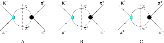
Figure B.1: Relevant diagrams for the calculation of FSI for $K^{+}\rightarrow\pi^{+}\pi^{+}\pi^{-}$. The square vertex is the weak vertex and the round one is the strong vertex

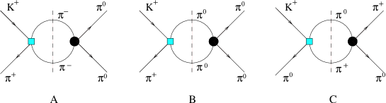
Figure B.2: Relevant diagrams for the calculation of FSI for $K^{+}\rightarrow\pi^{0}\pi^{0}\pi^{+}$. The square vertex is the weak vertex and the round one is the strong vertex.

We can distinguish the cases in which the weak vertex is of ${\cal O}(p^{4})$ and the strong vertex of order ${\cal O}(p^{2})$ and the inverse case in which the weak vertex is of order ${\cal O}(p^{2})$ and the strong vertex of order ${\cal O}(p^{4})$. In this paper we will not consider the weak vertices generated by the electroweak penguin. In Subsection B.4.1 we provide some notation. In Subsections B.4.2 and B.4.3 we report the calculation for the charged Kaon decays. An example of the calculation of the integrals that must be performed is given in Subsection B.4.4. Finally, in Subsection B.4.5 we give analytical results for the strong phases at NLO.

B.4.1 Notation

In order to be concise we use the functions $M_{i}$ for the weak amplitudes given in [64]. We define

$$\widetilde{M}_{i}(s) = \int_{-1}^{1}d\cos\theta\;\left.M_{i}(a(s)+b(s)\cos\theta)\right|_{p^{4}}\,,$$ (B.20)

$$\widetilde{M}_{i}^{s}(s) = \int_{-1}^{1}d\cos\theta\;\left.(a(s)+b(s)\cos\theta)M_{i}(a(s)+b(s)\cos\theta)\right|_{p^{4}}\,,$$ (B.21)

$$\widetilde{M}_{i}^{ss}(s) = \int_{-1}^{1}d\cos\theta\;\left.(a(s)+b(s)\cos\theta)^{2}M_{i}(a(s)+b(s)\cos\theta)\right|_{p^{4}}\,,$$ (B.22)

$$a(s) = \frac{1}{2}(m_{K}^{2}+3m_{\pi}^{2}-s)\,,$$

$$b(s) = \frac{1}{2}\sqrt{(s-4m_{\pi}^{2})\left(s-2(m_{K}^{2}+m_{\pi}^{2})+\frac{(m_{K}^{2}-m_{\pi}^{2})^{2}}{s}\right)}\,.$$ (B.23)

The amplitudes at ${\cal O}(p^{4})$ for the $\pi\pi\rightarrow\pi\pi$ scattering in a theory with three flavors can be found in [188]. We decompose the amplitudes in the various cases as follows. For the case $\pi^{+}\pi^{+}\rightarrow\pi^{+}\pi^{+}$ the amplitude at ${\cal O}(p^{4})$ is

$$\Pi_{1} = P_{1}(s)+P_{2}(s,t)+P_{2}(s,u).$$ (B.24)

For the case $\pi^{0}\pi^{0}\rightarrow\pi^{+}\pi^{-}$ the amplitude at ${\cal O}(p^{4})$ is

$$\Pi_{2} = P_{3}(s)+P_{4}(s,t)+P_{4}(s,u).$$ (B.25)

For the case $\pi^{+}\pi^{-}\rightarrow\pi^{+}\pi^{-}$ the amplitude at ${\cal O}(p^{4})$ is

$$\Pi_{3} = P_{5}(s)+P_{6}(s,t)+P_{6}(s,u)+P_{7}(s,t)-P_{7}(s,u).$$ (B.26)

Finally the amplitude $\pi^{0}\pi^{0}\rightarrow\pi^{0}\pi^{0}$ at ${\cal O}(p^{4})$ is

$$\Pi_{4} = P_{8}(s)+P_{8}(t)+P_{8}(u).$$ (B.27)

The value for the various $P_{i}$ can be deduced from [188]. In the following we use

$$\!\!\!\!\!\!\!\!\!\widetilde{P}^{(n,m)}_{i}(s) = \int_{-1}^{1}d\cos\theta\;s^{n}(c(s)(1-\cos\theta))^{m}P_{i}(s,c(s)(1-\cos\theta))\,,$$ (B.28)

$$\!\!\!\!\!\!\!\!\!\widehat{P}^{(n)}_{1,i}(s) = \int_{-1}^{1}d\cos\theta\;(c(s)(1-\cos\theta))^{n}P_{i}(c(s)(1+\cos\theta),c(s)(1-\cos\theta))\,,$$ (B.29)

$$\!\!\!\!\!\!\!\!\!\widehat{P}^{(n)}_{2,i}(s) = \int_{-1}^{1}d\cos\theta\;(c(s)(1-\cos\theta))^{n}P_{i}(c(s)(1-\cos\theta),s)\,,$$ (B.30)

$$\!\!\!\!\!\!\!\!\!c(s) = -\frac{1}{2}(s-4m_{\pi}^{2})\,.$$ (B.31)

Another function we use in the next subsections is $\sigma(s)$ which was defined already in (B.18).

B.4.2 Final State Interactions for $K^{+}\rightarrow\pi^{+}\pi^{+}\pi^{-}$

We first compute the contributions depicted in Figure B.1 in which the weak vertex is of ${\cal O}(p^{4})$ and the strong vertex of ${\cal O}(p^{2})$. The results for the diagrams A and B are

$${\rm Im}A^{(6,1)}_{W} = \frac{\sigma(s_{3})}{32\pi}\frac{(2m_{\pi}^{2}-s_{3})}{f_{\pi}^{2}}\left[\left.M_{10}(s_{3})\right|_{p^{4}}+\widetilde{M}_{11}(s_{3})+\widetilde{M}_{12}(s_{3})(m_{K}^{2}\right.$$ (B.32)

$$+3m_{\pi}^{2}-2s_{3})\left.-\widetilde{M}_{12}^{s}(s_{3})\right]\,,$$

$${\rm Im}A^{(6,2)}_{W} = \frac{\sigma(s_{1})}{32\pi}\frac{(s_{1}-m_{\pi}^{2})}{f_{\pi}^{2}}\left[\left.M_{7}(s_{1})\right|_{p^{4}}+\widetilde{M}_{8}(s_{1})+\widetilde{M}_{9}(s_{1})(m_{K}^{2}+3m_{\pi}^{2}-2s_{1})\right.$$ (B.33)

$$\left.-\widetilde{M}_{9}^{s}(s_{1})\right]+(s_{1}\leftrightarrow s_{2})\,,$$

respectively. For diagram C we have both $S$-wave and $P$-wave contributions. We get for them

$${\rm Im}A^{(6,3)}_{W,S} = \frac{\sigma(s_{1})}{64\pi}\frac{s_{1}}{f_{\pi}^{2}}\left[2\left.M_{11}(s_{1})\right|_{p^{4}}+\widetilde{M}_{11}(s_{1})+\widetilde{M}_{10}(s_{1})+\widetilde{M}_{12}^{s}(s_{1})\right.$$ (B.34)

$$\left.-\widetilde{M}_{12}(s_{1})(m_{K}^{2}+3m_{\pi}^{2}-2s_{1})\right]+(s_{1}\leftrightarrow s_{2})\,,$$

$${\rm Im}A^{(6,3)}_{W,P} = \frac{\sigma(s_{1})}{64\pi}\frac{1}{f_{\pi}^{2}}\frac{s_{1}(s_{3}-s_{2})}{s_{1}^{2}-2(m_{K}^{2}+m_{\pi}^{2})s_{1}+(m_{K}^{2}-m_{\pi}^{2})^{2}}\left[(s_{1}-(m_{K}^{2}+3m_{\pi}^{2}))\right.$$ (B.35)

$$\!\!\!\times(\widetilde{M}_{11}(s_{1})-\widetilde{M}_{10}(s_{1})+\widetilde{M}_{12}(s_{1})(2s_{1}-m_{K}^{2}-3m_{\pi}^{2}))+2\widetilde{M}^{s}_{11}(s_{1})$$

$$\!\!\!-2\widetilde{M}^{s}_{10}(s_{1})+\widetilde{M}^{s}_{12}(s_{1})(5s_{1}-3(m_{K}^{2}+3m_{\pi}^{2}))+2\widetilde{M}^{ss}_{12}(s_{1})$$

$$\!\!\!+\frac{8}{3}b^{2}(s_{1})\left.M_{12}(s_{1})\right|_{p^{4}}\Big{]}+(s_{1}\leftrightarrow s_{2})\,,$$

respectively.

Secondly, we report the calculation of the case in which the strong vertex is of ${\cal O}(p^{4})$ and the weak vertex is of ${\cal O}(p^{2})$. With analogous notation as above, we get

$${\rm Im}A^{(6,1)}_{\pi} = \frac{\sigma(s_{3})}{32\pi}\left.M_{10}(s_{3})\right|_{p^{2}}\ (P_{1}(s_{3})+\widetilde{P}^{(0,0)}_{2}(s_{3}))\,,$$ (B.36)

$${\rm Im}A^{(6,2)}_{\pi} = \frac{\sigma(s_{1})}{32\pi}\left.(M_{7}(s_{1})+M_{8}(s_{2})+M_{8}(s_{3}))\right|_{p^{2}}\,(P_{3}(s_{1})+\widetilde{P}^{(0,0)}_{4}(s_{1}))$$ (B.37)

$$\!\!\!+(s_{1}\leftrightarrow s_{2})\,,$$

$${\rm Im}A^{(6,3)}_{\pi,S} = \frac{\sigma(s_{1})}{32\pi}\left(\left.M_{10}(s_{3})\right|_{p^{2}}+\left.M_{10}(s_{2})\right|_{p^{2}}\right)(P_{5}(s_{1})+\widetilde{P}^{(0,0)}_{6}(s_{1}))$$ (B.38)

$$\!\!\!+(s_{1}\leftrightarrow s_{2})\,,$$

$${\rm Im}A^{(6,3)}_{\pi,P} = \frac{\sigma(s_{1})}{32\pi}\left(\left.M_{10}(s_{3})\right|_{p^{2}}-\left.M_{10}(s_{2})\right|_{p^{2}}\right)\frac{1}{s_{1}-4m_{\pi}^{2}}\Big{(}(s_{1}-4m_{\pi}^{2})\widetilde{P}_{7}^{(0,0)}(s_{1})$$ (B.39)

$$\!\!\!+2\widetilde{P}_{7}^{(0,1)}(s_{1})\Big{)}+(s_{1}\leftrightarrow s_{2})\,.$$

The final result for the Im$A^{(6)}$ is given by the sum

$${\rm Im}A^{(6)} = \sum_{i=1,2;\ j=W,\pi}{\rm Im}A^{(6,i)}_{j}+\sum_{j=W,\pi;\ k=S,P}{\rm Im}A^{(6,3)}_{j,k}\,.$$ (B.40)

The relation between this imaginary amplitude and the functions defined in Appendix B.1 is

$$\mbox{Im }A^{(6)}=\sum_{i=8,27}G_{i}\,C_{i}^{(6)}(s_{1},s_{2},s_{3})\,+\,\sum_{i=1,11}H_{i}^{(6)}(s_{1},s_{2},s_{3})\widetilde{K}_{i}\,.$$ (B.41)

This relation is also valid for $K^{+}\to\pi^{0}\pi^{0}\pi^{+}$.

B.4.3 Final State Interactions for $K^{+}\rightarrow\pi^{0}\pi^{0}\pi^{+}$

The calculation is analogous to the one for $K^{+}\rightarrow\pi^{+}\pi^{+}\pi^{-}$. The relevant graphs are depicted in Figure B.2. In the case in which the weak vertex is of ${\cal O}(p^{4})$, we get

$${\rm Im}A^{(6,1)}_{W} = \frac{\sigma(s_{3})}{32\pi}\frac{(s_{3}-m_{\pi}^{2})}{f_{\pi}^{2}}\left[2M_{11}(s_{3})+\widetilde{M}_{11}(s_{3})+\widetilde{M}_{10}(s_{3})-\widetilde{M}_{12}(s_{3})(m_{K}^{2}\right.$$ (B.42)

$$\left.+3m_{\pi}^{2}-2s_{3})+\widetilde{M}_{12}^{s}(s_{3})\right]\,,$$

$${\rm Im}A^{(6,2)}_{W} = \frac{\sigma(s_{3})}{32\pi}\frac{m_{\pi}^{2}}{f_{\pi}^{2}}\left[M_{7}(s_{3})+\widetilde{M}_{8}(s_{3})+\widetilde{M}_{9}(s_{3})(m_{K}^{2}+3m_{\pi}^{2}-2s_{3})\right.$$ (B.43)

$$\left.-\widetilde{M}_{9}^{s}(s_{3})\right]\,,$$

$${\rm Im}A^{(6,3)}_{W,S} = \frac{\sigma(s_{1})}{64\pi}\frac{(2m_{\pi}^{2}-s_{1})}{f_{\pi}^{2}}\left[2M_{8}(s_{1})+\widetilde{M}_{8}(s_{1})+\widetilde{M}_{7}(s_{1})-\widetilde{M}_{9}(s_{1})(m_{K}^{2}\right.$$ (B.44)

$$+3m_{\pi}^{2}-2s_{1})\left.+\widetilde{M}_{9}^{s}(s_{1})\right]+(s_{1}\leftrightarrow s_{2})\,.$$

Also in this case diagram C generates both $S$-wave and $P$-wave contributions. The P-wave contribution due to the diagram C in B.2 is

$${\rm Im}A^{(6,3)}_{W,P} = \frac{\sigma(s_{1})}{64\pi}\frac{1}{f_{\pi}^{2}}\frac{s_{1}(s_{3}-s_{2})}{s_{1}^{2}-2(m_{K}^{2}+m_{\pi}^{2})s_{1}+(m_{K}^{2}-m_{\pi}^{2})^{2}}\left[(s_{1}-(m_{K}^{2}+3m_{\pi}^{2}))\right.$$ (B.45)

$$\!\!\!\times(\widetilde{M}_{8}(s_{1})-\widetilde{M}_{7}(s_{1})+\widetilde{M}_{9}(s_{1})(2s_{1}-m_{K}^{2}-3m_{\pi}^{2}))+2\widetilde{M}^{s}_{8}(s_{1})$$

$$\!\!\!-2\widetilde{M}^{s}_{7}(s_{1})+\widetilde{M}^{s}_{9}(s_{1})(5s_{1}-3(m_{K}^{2}+3m_{\pi}^{2}))+2\widetilde{M}^{ss}_{9}(s_{1})$$

$$\!\!\!+\frac{8}{3}b^{2}(s_{1})M_{9}(s_{1})\Big{]}+(s_{1}\leftrightarrow s_{2})\,.$$

If the strong vertex is ${\cal O}(p^{4})$ and the weak vertex is order ${\cal O}(p^{2})$, we get

$${\rm Im}A^{(6,1)}_{\pi} = \frac{\sigma(s_{3})}{32\pi}\left.(M_{10}(s_{1})+M_{10}(s_{2}))\right|_{p^{2}}\ (P_{3}(s_{3})+\widetilde{P}^{(0,0)}_{4}(s_{3}))\,,$$ (B.46)

$${\rm Im}A^{(6,2)}_{\pi} = \frac{\sigma(s_{3})}{32\pi}\left.(M_{7}(s_{3})+M_{8}(s_{1})+M_{8}(s_{2}))\right|_{p^{2}}\,(P_{8}(s_{3})+\widetilde{P}^{(0,0)}_{8}(s_{3}))\,,$$

$${\rm Im}A^{(6,3)}_{\pi,S} = \frac{\sigma(s_{1})}{64\pi}\left.\left(2M_{8}(s_{1})+M_{8}(s_{2})+M_{8}(s_{3})+M_{7}(s_{2})+M_{7}(s_{3})\right)\right|_{p^{2}}$$ (B.48)

$$\!\!\!\times\Big{(}\widetilde{P}^{(0,0)}_{3}(s_{1})+\widehat{P}^{(0)}_{1,4}(s_{1})+\widetilde{P}^{(0)}_{2,4}(s_{1})\Big{)}+(s_{1}\leftrightarrow s_{2})\,,$$

$${\rm Im}A^{(6,3)}_{\pi,P} = \frac{\sigma(s_{1})}{64\pi}\left.\left(M_{7}(s_{3})-M_{8}(s_{3})-M_{7}(s_{2})+M_{8}(s_{2})\right)\right|_{p^{2}}\frac{1}{s_{1}-4m_{\pi}^{2}}$$ (B.49)

$$\!\!\!\times\Big{(}(s_{1}-4m_{\pi}^{2})(\widetilde{P}^{(0,0)}_{3}(s_{1})-\widehat{P}^{(0)}_{1,4}(s_{1})+\widetilde{P}^{(0)}_{2,4}(s_{1}))+2\widetilde{P}^{(1,0)}_{3}(s_{1})$$

$$\!\!\!-2\widetilde{P}^{(1)}_{1,4}(s_{1})+2\widehat{P}^{(1)}_{2,4}(s_{1})\Big{)}+(s_{1}\leftrightarrow s_{2})\,.$$

The total contribution is given by the sum of (B.40) with the proper right-hand side terms.

B.4.4 Integrals

The integrals necessary to compute the two-bubble FSI we discussed in the previous subsection can be calculated generalizing the method outlined in [189]. As an example we show the integration of the function

$$32\pi^{2}B(m_{1},m_{2},t) = C_{B}+\left\{\frac{2\eta\delta}{t}\ln\frac{\eta-\delta}{\eta+\delta}+\frac{\lambda}{t}\ln\frac{(\lambda-t)^{2}-\eta^{2}\delta^{2}}{(\lambda+t)^{2}-\eta^{2}\delta^{2}}\right\}$$ (B.50)

where $C_{B}$ is a term which does not depend on $t$,

$$C_{B} = 2\left(1-\ln\frac{\eta^{2}-\delta^{2}}{4\nu^{2}}\right)$$ (B.51)

and

$$\eta = m_{1}+m_{2}$$

$$\delta = m_{1}-m_{2}$$

$$\lambda = \sqrt{\left[\left(t-\eta^{2}\right)\left(t-\delta^{2}\right)\right]}\,.$$ (B.52)

In the center of mass frame one can define

$$Q = p_{K}+p_{\pi}=(\sqrt{s},0,0,0)$$

$$p_{\pi} = \frac{\sqrt{s}}{2}\left(\left(1-\frac{m_{K}^{2}-m_{\pi}^{2}}{s}\right),0,0,\sqrt{1-\frac{2(m_{K}^{2}+m_{\pi}^{2})}{s}+\frac{(m_{K}^{2}-m_{\pi}^{2})^{2}}{s^{2}}}\right)$$

where $p_{\pi}$ is the momentum of the external pion entering in the same vertex of the Kaon. The functions $B$ can also be generated in the strong vertex. In this case $p_{k}$ is the momentum of an external pion. The contribution to the imaginary part of the amplitude $A$ is

$${\rm Im}\,A=\frac{1}{32\pi}\sigma(s)\int_{-1}^{1}{\rm d}\,\cos\theta\,B[m_{1},m_{2},t]$$ (B.54)

with

$$t = a+b\cos\theta$$ (B.55)

and $a\equiv a(s)$, $b\equiv b(s)$ in (B.20). In order to solve the difficult part of the integral one can put

$$t=\frac{1}{2}\left[\eta^{2}+\delta^{2}-(\eta^{2}-\delta^{2})\frac{1+x^{2}}{2x}\right]\,.$$ (B.56)

In this way

$$\int_{-1}^{1}d\!\cos\theta\frac{\lambda}{t}\ln\frac{(\lambda-t)^{2}-\eta^{2}\delta^{2}}{(\lambda+t)^{2}-\eta^{2}\delta^{2}} = \frac{\eta^{2}-\delta^{2}}{2b}\int_{x_{\rm min}}^{x_{\rm max}}dx\;\frac{(1-x^{2})^{2}\ln x}{x^{2}\left(x^{2}+1-2x\alpha\right)}$$ (B.58)

$$= \frac{\eta^{2}-\delta^{2}}{2bx}\biggr{\{}-1-x^{2}-(1-x^{2})\ln x+\alpha x\ln^{2}x$$

$$\!\!\!+2x\sqrt{\alpha^{2}-1}\biggl{(}\ln x\ln\frac{1-\alpha+x\sqrt{a^{2}-1}}{1-\alpha-x\sqrt{a^{2}-1}}\biggr{.}$$

$$\!\!\!+Li_{2}\left(\frac{x}{\alpha+\sqrt{\alpha^{2}-1}}\right)$$

$$\!\!\!\left.\biggl{.}+Li_{2}\left(x(\alpha+\sqrt{\alpha^{2}-1})\right)\biggr{)}\biggr{\}}\right|_{x_{\rm min}}^{x_{\rm max}}$$

where

$$\alpha = {(\eta^{2}+\delta^{2})\over(\eta^{2}-\delta^{2})}$$

$$x_{\rm max} = \frac{2}{\eta^{2}-\delta^{2}}\left\{\frac{\eta^{2}+\delta^{2}}{2}-a-b+\frac{1}{2}\sqrt{(2(a+b)-(\eta^{2}+\delta^{2}))^{2}-(\eta^{2}-\delta^{2})^{2}}\right\}$$

$$x_{\rm min} = \frac{2}{\eta^{2}-\delta^{2}}\left\{\frac{\eta^{2}+\delta^{2}}{2}-a+b+\frac{1}{2}\sqrt{(2(a-b)-(\eta^{2}+\delta^{2}))^{2}-(\eta^{2}-\delta^{2})^{2}}\right\}\,.$$

In the case $m_{K}=m_{\pi}$, $a+b=0$ and one recovers the formulas of [189].

B.4.5 Analytical Results for the Dominant FSI Phases at NLO

The elements of the matrices defined in (4.44) have the next analytical expressions at NLO

$$\mathbb{R}^{\rm LO} = \left(\begin{array}[]{cc}R_{11}&R_{12}\\ R_{21}&R_{22}\end{array}\right)\,,$$ (B.62)

$$\delta_{2}^{\rm NLO} = \frac{\displaystyle\sum_{i=8,27,E}G_{i}\left(C_{i,1}^{(++-)}+C_{i,1}^{(00+)}\right)+\sum_{i=1,11}\left(H_{i,1}^{(6)(++-)}+H_{i,1}^{(6)(00+)}\right)\widetilde{K}_{i}}{\displaystyle\sum_{i=8,27,E}G_{i}\left(B_{i,1}^{(++-)}+B_{i,1}^{(00+)}\right)+\sum_{i=1,11}\left(H_{i,1}^{(4)(++-)}+H_{i,1}^{(4)(00+)}\right)\widetilde{K}_{i}}\,,$$ (B.63)

with

$$R_{11} = \frac{\left(-\beta_{1}+\frac{1}{2}\beta_{3}\right)^{\rm NR}\left(\alpha_{1}+\alpha_{3}\right)^{\rm R-NR}-\left(\beta_{1}+\beta_{3}\right)^{\rm NR}\left(-\alpha_{1}+\frac{1}{2}\alpha_{3}\right)^{\rm R-NR}}{\left(-\beta_{1}+\frac{1}{2}\beta_{3}\right)^{\rm NR}\left(\alpha_{1}+\alpha_{3}\right)^{\rm NR}-\left(\beta_{1}+\beta_{3}\right)^{\rm NR}\left(-\alpha_{1}+\frac{1}{2}\alpha_{3}\right)^{\rm NR}}\,,$$

$$R_{21} = \frac{\left(-\beta_{1}+\frac{1}{2}\beta_{3}\right)^{\rm NR}\left(\beta_{1}+\beta_{3}\right)^{\rm R-NR}-\left(\beta_{1}+\beta_{3}\right)^{\rm NR}\left(-\beta_{1}+\frac{1}{2}\beta_{3}\right)^{\rm R-NR}}{\left(-\beta_{1}+\frac{1}{2}\beta_{3}\right)^{\rm NR}\left(\alpha_{1}+\alpha_{3}\right)^{\rm NR}-\left(\beta_{1}+\beta_{3}\right)^{\rm NR}\left(-\alpha_{1}+\frac{1}{2}\alpha_{3}\right)^{\rm NR}}\ ,$$

$$R_{12} = -\frac{\left(-\alpha_{1}+\frac{1}{2}\alpha_{3}\right)^{\rm NR}\left(\alpha_{1}+\alpha_{3}\right)^{\rm R-NR}-\left(\alpha_{1}+\alpha_{3}\right)^{\rm NR}\left(-\alpha_{1}+\frac{1}{2}\alpha_{3}\right)^{\rm R-NR}}{\left(-\beta_{1}+\frac{1}{2}\beta_{3}\right)^{\rm NR}\left(\alpha_{1}+\alpha_{3}\right)^{\rm NR}-\left(\beta_{1}+\beta_{3}\right)^{\rm NR}\left(-\alpha_{1}+\frac{1}{2}\alpha_{3}\right)^{\rm NR}}\,,$$

$$R_{22} = -\frac{\left(-\alpha_{1}+\frac{1}{2}\alpha_{3}\right)^{\rm NR}\left(\beta_{1}+\beta_{3}\right)^{\rm R-NR}-\left(\alpha_{1}+\alpha_{3}\right)^{\rm NR}\left(-\beta_{1}+\frac{1}{2}\beta_{3}\right)^{\rm R-NR}}{\left(-\beta_{1}+\frac{1}{2}\beta_{3}\right)^{\rm NR}\left(\alpha_{1}+\alpha_{3}\right)^{\rm NR}-\left(\beta_{1}+\beta_{3}\right)^{\rm NR}\left(-\alpha_{1}+\frac{1}{2}\alpha_{3}\right)^{\rm NR}}\,,$$ (B.64)

The definitions of $\alpha_{1}$, $\alpha_{3}$, $\beta_{1}$ and $\beta_{3}$ are in (4.4.1) and the values of their relevant combinations are

$$\left(-\alpha_{1}+\frac{1}{2}\alpha_{3}\right)^{\rm NR} = \sum_{i=8,27,E}G_{i}B_{i,0}^{(00+)}+\sum_{i=1,11}H_{i,0}^{(4)(00+)}\widetilde{K}_{i}\,,$$

$$\left(-\alpha_{1}+\frac{1}{2}\alpha_{3}\right)^{\rm R-NR} = \sum_{i=8,27,E}G_{i}C_{i,0}^{(00+)}+\sum_{i=1,11}H_{i,0}^{(6)(00+)}\widetilde{K}_{i}\,,$$

$$\left(-\beta_{1}+\frac{1}{2}\beta_{3}\right)^{\rm NR} = \frac{1}{2}\left[\sum_{i=8,27,E}G_{i}\left(B_{i,1}^{(++-)}-B_{i,1}^{(00+)}\right)\right.$$

$$\left.+\sum_{i=1,11}\left(H_{i,1}^{(4)(++-)}-H_{i,1}^{(4)(00+)}\right)\widetilde{K}_{i}\right]\,,$$

$$\left(-\beta_{1}+\frac{1}{2}\beta_{3}\right)^{\rm R-NR} = \frac{1}{2}\left[\sum_{i=8,27,E}G_{i}\left(C_{i,1}^{(++-)}-C_{i,1}^{(00+)}\right)\right.$$

$$\left.+\sum_{i=1,11}\left(H_{i,1}^{(6)(++-)}-H_{i,1}^{(6)(00+)}\right)\widetilde{K}_{i}\right]\,,$$

$$\left(\alpha_{1}+\alpha_{3}\right)^{\rm NR} = \sum_{i=8,27,E}G_{i}B_{i,0}^{(+-0)}+\sum_{i=1,11}H_{i,0}^{(4)(+-0)}\widetilde{K}_{i}\,,$$

$$\left(\alpha_{1}+\alpha_{3}\right)^{\rm R-NR} = \sum_{i=8,27,E}G_{i}C_{i,0}^{(+-0)}+\sum_{i=1,11}H_{i,0}^{(6)(+-0)}\widetilde{K}_{i}\,,$$

$$\left(\beta_{1}+\beta_{3}\right)^{\rm NR} = -\frac{1}{2}\left[\sum_{i=8,27,E}G_{i}B_{i,1}^{(+-0)}+\sum_{i=1,11}H_{i,1}^{(4)(+-0)}\widetilde{K}_{i}\right]\,,$$

$$\left(\beta_{1}+\beta_{3}\right)^{\rm R-NR} = \frac{1}{2}\left[\sum_{i=8,27,E}G_{i}C_{i,1}^{(+-0)}+\sum_{i=1,11}H_{i,1}^{(6)(+-0)}\widetilde{K}_{i}\right]\,.$$ (B.65)

where the functions $B_{i,0(1)}$, $C_{i,0(1)}$ and $H_{i,0(1)}$ are those obtained form the expansion in (B.9) of the corresponding full quantities that can be found in Appendix B.3.

Disregarding the tiny CP-violating (less than 1%) and the effects of order $e^{2}p^{2}$ (the loop contribution is less than 2%), we obtain the numbers in (4.4.1).

Appendix C Some Short-Distance Relations for Three-point Functions

We calculated or recalculated several short-distance behaviours of three-point functions in [11]. The results are

$$\lim_{\lambda\to\infty}\Pi^{PSP}(\lambda p_{1},\lambda p_{2})^{\chi}=\frac{\langle\overline{q}q\rangle_{\chi}}{2\lambda^{2}}\left\{\frac{p_{2}^{2}}{q^{2}p_{1}^{2}}+\frac{q^{2}}{p_{1}^{2}p_{2}^{2}}-\frac{p_{1}^{2}}{q^{2}p_{2}^{2}}-\frac{2}{p_{1}^{2}}\right\}$$ (C.1)

$$\lim_{\lambda\to\infty}\Pi^{SVV}(\lambda p_{1},\lambda p_{2})^{\chi}=\frac{\langle\overline{q}q\rangle_{\chi}}{2\lambda^{2}q^{2}p_{1}^{2}p_{2}^{2}}\Bigg{\{}-4p_{2}^{2}\,p_{1\mu}p_{1\nu}-2(p_{1}^{2}+p_{2}^{2}-q^{2})\,p_{1\mu}p_{2\nu}$$ (C.2)

$$-2(p_{1}^{2}+p_{2}^{2}+q^{2})\,p_{2\mu}p_{1\nu}-4p_{1}^{2}\,p_{2\mu}p_{2\nu}+\left(q^{4}-(p_{1}^{2}-p_{2}^{2})^{2}\right)\,g_{\mu\nu}\Bigg{\}}$$

$$\lim_{\lambda\to\infty}\Pi^{PVA}(\lambda p_{1},\lambda p_{2})^{\chi}=\frac{i\langle\overline{q}q\rangle_{\chi}}{2\lambda^{2}q^{2}p_{1}^{2}p_{2}^{2}}\Bigg{\{}4p_{2}^{2}\,p_{1\mu}p_{1\nu}-2(q^{2}+p_{1}^{2}-p_{2}^{2})\,p_{1\mu}p_{2\nu}$$ (C.3)

$$+2(q^{2}+p_{2}^{2}-p_{1}^{2})\,p_{2\mu}p_{1\nu}-4p_{1}^{2}\,p_{2\mu}p_{2\nu}+\left(p_{2}^{4}-(p_{1}^{2}-q^{2})^{2}\right)\,g_{\mu\nu}\Bigg{\}}$$

Some of these have been mentioned in Refs. [133, 160].

The following were first calculated to our knowledge in [11]

$$\lim_{\lambda\to\infty}\left(\Pi^{PAS}(\lambda p_{1},\lambda p_{2})^{\chi}+\Pi^{SAP}(\lambda p_{1},\lambda p_{2})^{\chi}\right)\,=\,i4\pi\alpha_{S}\frac{N_{c}^{2}-1}{N_{c}^{2}}\frac{\langle\overline{q}q\rangle_{\chi}^{2}}{\lambda^{5}}$$ (C.4)

$$\times\left\{\frac{2p_{1\mu}}{p_{1}^{2}}\left(\frac{1}{q^{4}}+\frac{1}{p_{2}^{4}}+\frac{1}{p_{2}^{2}q^{2}}\right)+\frac{p_{2\mu}}{p_{2}^{2}}\left(\frac{-1}{q^{4}}+\frac{1}{p_{2}^{2}q^{2}}\right)+\frac{q_{\mu}}{q^{2}}\left(\frac{1}{p_{2}^{4}}-\frac{1}{p_{2}^{2}q^{2}}\right)\right\}$$

$$\lim_{\lambda\to\infty}\lim_{m_{q}\to 0}\frac{\partial}{\partial m_{i}}\left(\Pi^{PAS}(\lambda p_{1},\lambda p_{2})^{ijk}+\Pi^{SAP}(\lambda p_{1},\lambda p_{2})^{ijk}\right) = -2i\langle\overline{q}q\rangle_{\chi}\frac{p_{2\mu}}{\lambda^{3}p_{2}^{2}q^{2}}\,,$$

$$\lim_{\lambda\to\infty}\lim_{m_{q}\to 0}\frac{\partial}{\partial m_{j}}\left(\Pi^{PAS}(\lambda p_{1},\lambda p_{2})^{ijk}+\Pi^{SAP}(\lambda p_{1},\lambda p_{2})^{ijk}\right) = 2i\langle\overline{q}q\rangle_{\chi}\frac{p_{1\mu}}{\lambda^{3}p_{1}^{2}}\left(\frac{1}{q^{2}}+\frac{1}{p_{2}^{2}}\right)\,,$$

$$\lim_{\lambda\to\infty}\lim_{m_{q}\to 0}\frac{\partial}{\partial m_{k}}\left(\Pi^{PAS}(\lambda p_{1},\lambda p_{2})^{ijk}+\Pi^{SAP}(\lambda p_{1},\lambda p_{2})^{ijk}\right) = 2i\langle\overline{q}q\rangle_{\chi}\frac{q_{\mu}}{\lambda^{3}p_{2}^{2}q^{2}}\,.$$ (C.5)

Bibliography

- [1] J. H. Christenson, J. W. Cronin, V. L. Fitch and R. Turlay, Phys. Rev. Lett. 13 (1964) 138.
- [2] B. Aubert et al. [BABAR Collaboration], Phys. Rev. Lett. 87 (2001) 091801 [arXiv:hep-ex/0107013].
- [3] K. Abe et al. [Belle Collaboration], Phys. Rev. Lett. 87 (2001) 091802 [arXiv:hep-ex/0107061].
- [4] S. Weinberg, PhysicaA 96 (1979) 327.
- [5] J. Gasser and H. Leutwyler, Annals Phys. 158 (1984) 142; Nucl. Phys. B 250 (1985) 465.
- [6] S. Chen, M. Davier, E. Gámiz, A. Hocker, A. Pich and J. Prades, Eur. Phys. J. C 22 (2001) 31 [arXiv:hep-ph/0105253].
- [7] E. Gámiz, M. Jamin, A. Pich, J. Prades and F. Schwab, J. High Energy Phys. 01 (2003) 060 [arXiv:hep-ph/0212230]; M. Jamin, arXiv:hep-ph/0309147.
- [8] E.. Gámiz, J. Prades and I. Scimemi, J. High Energy Phys. 10 (2003) 042 [arXiv:hep-ph/0309172].
- [9] J. Bijnens, E. Gámiz and J. Prades, J. High Energy Phys. 10 (2001) 009 [arXiv:hep-ph/0108240]; E. Gámiz, J. Prades and J. Bijnens, Nucl. Phys. B (Proc. Suppl.) 126 (2003) 195 [arXiv:hep-ph/0209089].
- [10] J. Bijnens, E. Gámiz and J. Prades, arXiv:hep-ph/0309216.
- [11] J. Bijnens, E. Gámiz, E. Lipartia and J. Prades, J. High Energy Phys. 04 (2003) 055 [arXiv:hep-ph/0304222].
- [12] S. L. Glashow, Nucl. Phys. 22 (1961) 579.
- [13] S. Weinberg, Phys. Rev. Lett. 19 (1967) 1264.
- [14] A. Salam, Originally printed in *Svartholm: Elementary Particle Theory, Proceedings of the Nobel Symposioum Held 1968 at Lerum, Sweden*, Stockholm 1968, 367-377
- [15] S. L. Glashow, J. Iliopoulos and L. Maiani, Phys. Rev. D 2 (1970) 1285.
-
[16]
O. W. Greenberg,
Phys. Rev. Lett. 13 (1964) 598;
M. Y. Han and Y. Nambu, Phys. Rev. 139 (1965) B1006;
H. Fritzsch, M. Gell-Mann and H. Leutwyler, Phys. Lett. B 47 (1973) 365. - [17] A. Pich, arXiv:hep-ph/0206011; eConf C0209101 (2002) TU01 [arXiv:hep-ph/0210445].
-
[18]
Y. Fukuda et al. [Super-Kamiokande Collaboration],
Phys. Rev. Lett. 81 (1998) 1562
[arXiv:hep-ex/9807003];
Q. R. Ahmad et al. [SNO Collaboration], Phys. Rev. Lett. 87 (2001) 071301 [arXiv:nucl-ex/0106015];
M. H. Ahn et al. [K2K Collaboration], Phys. Rev. Lett. 90 (2003) 041801 [arXiv:hep-ex/0212007];
K. Eguchi et al. [KamLAND Collaboration], Phys. Rev. Lett. 90 (2003) 021802 [arXiv:hep-ex/0212021]. - [19] A. Pich, arXiv:hep-ph/9412274, arXiv:hep-ph/9601202, arXiv:hep-ph/9610243, arXiv:hep-ph/0001118; Nucl. Phys. B (Proc. Suppl.) 66 (1998) 456 [arXiv:hep-ph/9709441], 81 (2000) 183 [arXiv:hep-ph/9910390], 98 (2001) 385 [arXiv:hep-ph/0012297].
- [20] W. A. Bardeen, A. J. Buras and J. M. Gerard, Phys. Lett. B 192 (1987) 138; Nucl. Phys. B 293 (1987) 787.
- [21] E. Pallante, A. Pich and I. Scimemi, Nucl. Phys. B 617 (2001) 441 [arXiv:hep-ph/0105011].
- [22] K. Hagiwara et al. [Particle Data Group Collaboration], Phys. Rev. D 66 (2002) 010001.
- [23] A. J. Buras and M. Jamin, arXiv:hep-ph/0306217.
-
[24]
P. Colangelo, F. De Fazio, G. Nardulli and N. Paver,
Phys. Lett. B 408 (1997) 340
[arXiv:hep-ph/9704249];
M. Jamin, Nucl. Phys. Proc. Suppl. 64 (1998) 250 [arXiv:hep-ph/9709484];
M. Eidemuller, M. Jamin and F. Schwab, arXiv:hep-ph/0310185. - [25] M. Jamin, J. A. Oller and A. Pich, Eur. Phys. J. C 24 (2002) 237 [arXiv:hep-ph/0110194].
- [26] K. Maltman and J. Kambor, Phys. Rev. D 65 (2002) 074013 [arXiv:hep-ph/0108227].
-
[27]
V. Lubicz,
Nucl. Phys. B (Proc. Suppl.) 94 (2001) 116
[arXiv:hep-lat/0012003];
R. Gupta and K. Maltman, Int. J. Mod. Phys. A 16S1B (2001) 591 [arXiv:hep-ph/0101132]. - [28] H. Wittig, Nucl. Phys. B (Proc. Suppl.) 119 (2003) 59 [arXiv:hep-lat/0210025].
- [29] T. Kaneko, Nucl. Phys. B (Proc. Suppl.) 106 (2002) 133 [hep-lat/0111005].
-
[30]
K. G. Chetyrkin, J. H. Kühn and A. A. Pivovarov,
Nucl. Phys. B 533 (1998) 473
[arXiv:hep-ph/9805335];
J. G. Körner, F. Krajewski and A. A. Pivovarov, Eur. Phys. J. C 20 (2001) 259 [arXiv:hep-ph/0003165];
M. Davier, S. M. Chen, A. Hocker, J. Prades and A. Pich, Nucl. Phys. B (Proc. Suppl.) 98 (2001) 319. - [31] R. Barate et al, [ALEPH Collaboration] Eur. Phys. J. C 4 (1998) 409.
- [32] J. Prades and A. Pich, Nucl. Phys. B (Proc. Suppl.) 74 (1999) 309 [arXiv:hep-ph/9811263]; Nucl. Phys. B (Proc. Suppl.) 86 (2000) 236 [arXiv:hep-ph/9909559];
- [33] J. Kambor and K. Maltman, Phys. Rev. D 62 (2000) 093023 [arXiv:hep-ph/0005156];
- [34] M. Jamin, J. A. Oller and A. Pich, Nucl. Phys. B 587 (2000) 331 [arXiv:hep-ph/0006045];
- [35] M. Jamin, J. A. Oller and A. Pich, Nucl. Phys. B 622 (2002) 279 [hep-ph/0110193].
- [36] G. Ecker, J. Gasser, H. Leutwyler, A. Pich and E. de Rafael, Phys. Lett. B 223 (1989) 425.
- [37] G. Ecker, J. Gasser, A. Pich and E. de Rafael, Nucl. Phys. B 321 (1989) 311.
- [38] M. Gell-Mann, R. J. Oakes and B. Renner, Phys. Rev. 175 (1968) 2195.
- [39] M. C. Gonzalez-Garcia and Y. Nir, Rev. Mod. Phys. 75, 345 (2003) [arXiv:hep-ph/0202058].
- [40] N. Cabibbo, Phys. Rev. Lett. 10 (1963) 531.
- [41] M. Kobayashi and T. Maskawa, Prog. Theor. Phys. 49 (1973) 652.
- [42] L. Wolfenstein, Phys. Rev. Lett. 51 (1983) 1945. Z. Phys. C 29 (1985) 491.
- [43] H. Fritzsch and Z. -z. Xing, Prog. Part. Nucl. Phys. 45 (2000) 1 [arXiv:hep-ph/9912358].
- [44] M. Battaglia et al., arXiv:hep-ph/0304132.
- [45] C. Jarlskog, Phys. Rev. Lett. 55 (1985) 1039;
- [46] A. Pich, arXiv:hep-ph/9312297.
- [47] P. Krawczyk, D. London, R. D. Peccei and H. Steger, Nucl. Phys. B 307 (1988) 19.
- [48] A. J. Buras, arXiv:hep-ph/0307203.
- [49] Y. Nir, Nucl. Phys. B (Proc. Suppl.) 117 (2003) 111 [arXiv:hep-ph/0208080].
- [50] K. Abe et al. [BELLE Collaboration], Phys. Rev. D 67 (2003) 031102 [arXiv:hep-ex/0212062].
- [51] B. Aubert et al. [BABAR Collaboration], arXiv:hep-ex/0303046.
- [52] K. Abe, arXiv:hep-ex/0308072.
- [53] E. de Rafael, arXiv:hep-ph/9502254.
- [54] A. J. Buras, M. Jamin and P. H. Weisz, Nucl. Phys. B 347 (1990) 491;
- [55] J. Urban, F. Krauss, U. Jentschura and G. Soff, Nucl. Phys. B 523 (1998) 40 [arXiv:hep-ph/9710245].
- [56] S. Herrlich and U. Nierste, Nucl. Phys. B 476 (1996) 27 [arXiv:hep-ph/9604330].
- [57] S. Herrlich and U. Nierste, Nucl. Phys. B 419 (1994) 292 [arXiv:hep-ph/9310311].
- [58] T. Inami and C. S. Lim, Prog. Theor. Phys. 65 (1981) 297 [Erratum-ibid. 65 (1981) 1772].
- [59] M. Ciuchini, E. Franco, F. Parodi, V. Lubicz, L. Silvestrini and A. Stocchi, eConf C0304052 (2003) WG306 [arXiv:hep-ph/0307195].
- [60] H. Burkhardt et al. [NA31 Collaboration], Phys. Lett. B 206 (1988) 169;
- [61] J.R. Batley et al. [NA48 Collaboration], Phys. Lett. B 544 (2002) 97 [arXiv:hep-ex/0208009].
- [62] A. Alavi-Harati et al. [KTeV Collaboration], Phys. Rev. D 67 (2003) 012005 [arXiv:hep-ex/0208007].
- [63] G. D. Barr et al. [NA31 Collaboration], Phys. Lett. B 317 (1993) 233; Ł. K. Gibbons et al., Phys. Rev. Lett. 70 (1993) 1203; A. Alavi-Harati et al. [KTeV Collaboration], Phys. Rev. Lett. 83 (1999) 22 [arXiv:hep-ex/9905060]; A. Lai et al. [NA48 Collaboration], Eur. Phys. J. C 22 (2001) 231 [arXiv:hep-ex/0110019].
- [64] J. Bijnens, P. Dhonte and F. Persson, Nucl. Phys. B 648 (2003) 317 [arXiv:hep-ph/0205341].
- [65] A. J. Buras and P. H. Weisz, Nucl. Phys. B 333 (1990) 66; A. J. Buras, M. Jamin, E. Lautenbacher and P. H. Weisz, Nucl. Phys. B 370 (1992) 69 [Addendum-ibid. B 375 (1992) 501]; Nucl. Phys. B 400 (1993) 37 [hep-ph/9211304]; Nucl. Phys. B 400 (1993) 75 [hep-ph/9211321]; A. J. Buras, M. Jamin and M. E. Lautenbacher, Nucl. Phys. B 408 (1993) 209 [arXiv:hep-ph/9303284].
- [66] M. Ciuchini, E. Franco, G. Martinelli and L. Reina, Phys. Lett. B 301 (1993) 263 [arXiv:hep-ph/9212203]; Nucl. Phys. B 415 (1994) 403 [hep-ph/9304257].
- [67] A. J. Buras, arXiv:hep-ph/9806471.
- [68] J. Bijnens, arXiv:hep-ph/0204068.
- [69] G. Buchalla, A. J. Buras and M. E. Lautenbacher, Rev. Mod. Phys. 68 (1996) 1125 [hep-ph/9512380].
- [70] V. Cirigliano, A. Pich, G. Ecker and H. Neufeld, “Isospin violation in epsilon’,” Phys. Rev. Lett. 91 (2003) 162001 [arXiv:hep-ph/0307030]; arXiv:hep-ph/0310351.
-
[71]
J. F. Donoghue, E. Golowich, B. R. Holstein and J. Trampetic,
Phys. Lett. B 179 (1986) 361
[Erratum-ibid. 188B (1987) 511];
H. Y. Cheng, Phys. Lett. B 201 (1988) 155;
M. Lusignoli, Nucl. Phys. B 325 (1989) 33;
A. J. Buras and J. M. Gerard, Phys. Lett. B 192 (1987) 156. - [72] J. Bijnens and J. Prades, J. High Energy Phys. 06 (2000) 035 [arXiv:hep-ph/0005189]; Nucl. Phys. B (Proc. Suppl.) 96 (2001) 354 [arXiv:hep-ph/0010008]; arXiv:hep-ph/0009156; arXiv:hep-ph/0009155.
- [73] J. Bijnens and J. Prades, Nucl. Phys. B 444 (1995) 523 [hep-ph/9502363]; Phys. Lett. B 342 (1995) 331 [hep-ph/9409255].
- [74] J. Bijnens and J. Prades, J. High Energy Phys. 01 (1999) 023 [arXiv:hep-ph/9811472]; J. Prades, Nucl. Phys. B (Proc. Suppl.) 86 (2000) 294 [arXiv:hep-ph/9909245]; J. Bijnens, arXiv:hep-ph/9907514.
- [75] J. Bijnens and J. Prades, J. High Energy Phys. 01 (2000) 002 [hep-ph/9911392].
- [76] E. Pallante and A. Pich, Nucl. Phys. B 592 (2001) 294 [arXiv:hep-ph/0007208]; Phys. Rev. Lett. 84 (2000) 2568 [arXiv:hep-ph/9911233].
- [77] J. Bijnens, E. Pallante and J. Prades, Nucl. Phys. B 521 (1998) 305 [arxiv:hep-ph/9801326].
- [78] V. Cirigliano and E. Golowich, Phys. Lett. B 475 (2000) 351 [arXiv:hep-ph/9912513]; Phys. Rev. D 65 (2002) 054014 [arXiv:hep-ph/0109265].
- [79] J. Bijnens and M. B. Wise, Phys. Lett. B 137 (1984) 245.
- [80] J. F. Donoghue and E. Golowich, Phys. Lett. B 478 (2000) 172 [hep-ph/9911309].
- [81] S. Narison, Nucl. Phys. B 593 (2001) 3 [hep-ph/0004247]; Nucl. Phys. B (Proc. Suppl.) 96 (2001) 364 [hep-ph/0012019].
- [82] M. Knecht, S. Peris and E. de Rafael, Phys. Lett. B 508 (2001) 117 [arXiv:hep-ph/0102017]; M. Knecht, Proceedings High-Energy Physics (HEP 2001), 226; S. Peris, arXiv:hep-ph/0204181;
- [83] V. Cirigliano, J. F. Donoghue, E. Golowich and K. Maltman, Phys. Lett. B 522 (2001) 245 [arXiv:hep-ph/0109113].
- [84] V. Cirigliano, Talk at QCD ’02, Montpellier, arXiv:hep-ph/0209332; E. Golowich, Talk at ICHEP ’02, Amsterdam.
- [85] V. Cirigliano, J. F. Donoghue, E. Golowich and K. Maltman, arXiv:hep-ph/0209332; Phys. Lett. B 555 (2003) 71 [arXiv:hep-ph/0211420].
- [86] J. I. Noaki et al. [CP-PACS Collaboration], Phys. Rev. D 68 (2003) 014501 [arXiv:hep-lat/0108013].
- [87] T. Blum et al. [RBC Collaboration], arXiv:hep-lat/0110075.
- [88] T. Bhattacharya, G. T. Fleming, G. Kilcup, R. Gupta, W. Lee and S. Sharpe, arXiv:hep-lat/0309105.
- [89] P. Boucaud, V. Gimenez, C. J. Lin, V. Lubicz, G. Martinelli, M. Papinutto and C. T. Sachrajda [SPQcdR Collaboration], arXiv:hep-lat/0309128.
- [90] T. Hambye, S. Peris and E. de Rafael, J. High Energy Phys. 05 (2003) 027 [arXiv:hep-ph/0305104].
- [91] M. Ciuchini et al., arXiv:hep-ph/9910237; Nucl. Phys. B 523 (1998) 501 [arXiv:hep-ph/9711402]; Nucl. Phys. B 415 (1994) 403 [arXiv:hep-ph/9304257]; Phys. Lett. B 301 (1993) 263 [arXiv:hep-ph/9212203].
- [92] A. J. Buras, M. Jamin and M. E. Lautenbacher, Nucl. Phys. B 408 (1993) 209 [arXiv:hep-ph/9303284].
- [93] S. Bertolini, J. O. Eeg, M. Fabbrichesi and E. I. Lashin, Nucl. Phys. B 514 (1998) 93 [arXiv:hep-ph/9706260]; Phys. Rev. D 63 (2001) 056009 [arXiv:hep-ph/0002234].
- [94] T. Hambye, G.O. Köhler, E.A. Paschos and P.H. Soldan, Nucl. Phys. B 564 (2000) 391 [arXiv:hep-ph/9906434]; T. Hambye, G.O. Köhler, E.A. Paschos, P.H. Soldan and W.A. Bardeen, Phys. Rev. D 58 (1998) 014017 [arXiv:hep-ph/9802300].
-
[95]
G. ’t Hooft,
Nucl. Phys. B 72 (1974) 461;
A. V. Manohar, hep-ph/9802419, Les Houches Summer School in Theoretical Physics, Session 68: Probing the Standard Model of Particle Interactions, Les Houches, France, 28 Jul - 5 Sep 1997 F. David and R. Gupta eds. -
[96]
W. A. Bardeen, J. Bijnens and J. M. Gerard,
Phys. Rev. Lett. 62 (1989) 1343;
J. Bijnens, J. M. Gerard and G. Klein, Phys. Lett. B 257 (1991) 191;
J. P. Fatelo and J. M. Gerard, Phys. Lett. B 347 (1995) 136. - [97] A. Pich and E. de Rafael, Nucl. Phys. B 358 (1991) 311.
- [98] G. Ecker, G. Isidori, G. Müller, H. Neufeld and A. Pich, Nucl. Phys. B 591 (2000) 419 [arXiv:hep-ph/0006172].
- [99] V. Cirigliano, J. F. Donoghue and E. Golowich, Phys. Lett. B 450 (1999) 241; Phys. Rev. D 61 (2000) 093001 [Erratum-ibid. D 63 (2001) 059903] [arXiv:hep-ph/9907341]; V. Cirigliano, J. F. Donoghue and E. Golowich, Phys. Rev. D 61 (2000) 093002 [arXiv:hep-ph/9909473]; V. Cirigliano and E. Golowich, Phys. Lett. B 475 (2000) 351 [arXiv:hep-ph/9912513].
- [100] S. Peris, arXiv:hep-ph/0310063.
- [101] J.A. Cronin, Phys. Rev. 161 (1967) 1483; B.R. Holstein, ibidem 183 (1969) 1228; T.J. Devlin and J.O. Dickey, Rev. Mod. Phys. 51 (1979) 237.
- [102] J.F. Donoghue, E. Golowich, B.R. Holstein, Phys. Rev. D 30 (1984) 587; H.-Y. Cheng, C.Y. Cheung, W.B. Yeung, Mod. Phys. Lett. A 4 (1989) 869; Z. Phys. C 43 (1989) 391; S. Fajfer, J.-M. Gérard, Z. Phys. C 42 (1989) 425.
- [103] J. Kambor, J. Missimer and D. Wyler, Phys. Lett. B 261 (1991) 496.
- [104] J. Kambor, J. Missimer and D. Wyler, Nucl. Phys. B 346 (1990) 17.
- [105] J. Kambor, J.F. Donoghue, B.R. Holstein, J. Missimer and D. Wyler, Phys. Rev. Lett. 68 (1992) 1818.
- [106] B.R. Holstein Phys. Rev. 177 (1969) 2417;
- [107] L.-F. Li and L. Wolfenstein, Phys. Rev. D 21 (1980) 178.
- [108] C. Avilez, Phys. Rev. D 23 (1981) 1124.
- [109] B. Grinstein, S.-J. Rey and M.B. Wise, Phys. Rev. D 33 (1986) 1495.
- [110] J.F. Donoghue, B.R. Holstein and G. Valencia, Phys. Rev. D 36 (1987) 798.
-
[111]
A.A. Bel’kov, A.V. Lanyov, G. Bohm and D. Ebert,
Phys. Lett. B 232 (1989) 118;
A.A. Bel’kov, G. Bohm, D. Ebert, A.V. Lanyov and A. Schaale, Int. J. Mod. Phys. A 7 (1992) 4757. - [112] G. D’Ambrosio, G. Isidori and N. Paver, Phys. Lett. B 273 (1991) 497.
- [113] G. Isidori, L. Maiani and A. Pugliese, Nucl. Phys. B 381 (1992) 522.
- [114] L. Maiani, G. Pancheri and N. Paver, “The Second Daphne Physics Handbook. Vol. 1, 2,”
- [115] E.P. Shabalin, Talk at 17th Rencontres de Physique de la Vallee d’Aoste on Results and Perspectives in Particle Physics, La Thuile, Val d’Aosta, Italy, March 9-15 (2003), arXiv:hep-ph/0305320.
- [116] E.P. Shabalin, Nucl. Phys. B 409 (1993) 87; ITEP-92-6; Phys. Atom. Nucl. 61 (1998) 1372 [Yad. Fiz. 61 (1998) 1478].
- [117] G. D’Ambrosio, G. Isidori, A. Pugliese and N. Paver, Phys. Rev. D 50 (1994) 5767 [Erratum-ibid. D 51 (1995) 3975] [arXiv:hep-ph/9403235].
- [118] E. Gámiz, J. Prades and I. Scimemi, Invited talk at 38th Rencontres de Moriond on Electroweak Interactions and Unified Theories, Les Arcs, France, March 15-22 (2003), arXiv:hep-ph/0305164.
- [119] I.V. Ajinenko et al., Phys. Lett. B 567 (2003) 159 [arXiv:hep-ex/0205027].
- [120] R. Wanke, Talk at 38th Rencontres de Moriond on Electroweak Interactions and Unified Theories, Les Arcs, France, March 15-22 (2003), arXiv:hep-ex/0305059; C. Cheshkov, Talk at 38th Rencontres de Moriond on QCD, Les Arcs, France, March 23-26 (2003), arXiv:hep-ex/0306012.
- [121] A. Aloisio et al. [KLOE Collaboration], arXiv:hep-ex/0307054; M. Primavera, Talk at Workshop on Chiral Dynamics 2003: Theory and Experiment, Bonn, Germany, September 8-13 (2003).
- [122] J. Wess and B. Zumino, Phys. Lett. B 37 (1971) 95.
- [123] E. Witten, Nucl. Phys. B 223 (1983) 422.
- [124] J. Prades and A. Pich, Phys. Lett. B 245 (1990) 117; J. Prades, Nucl. Phys. B (Proc. Suppl.) 23B (1991) 301; A. Pich, J. Prades and P. Yepes, Nucl. Phys. B 388 (1992) 31.
- [125] G. Ecker, Lectures given at the Advanced School on QCD 2000, Benasque, (Huesca), Spain, hep-ph/0011026; A. Pich, Lectures at Les Houches Summer School in Theoretical Physics, Session 68: Probing the Standard Model of Particle Interactions, Les Houches, France, arxiv:hep-ph/9806303.
- [126] G. Ecker, Prog. Part. Nucl. Phys. 35 (1995) 1 [arXiv:hep-ph/9501357]; A. Pich, Rept. Prog. Phys. 58 (1995) 563 [arXiv:hep-ph/9502366].
- [127] G. Amorós, J. Bijnens and P. Talavera, Nucl. Phys. B 602 (2001) 87 [hep-ph/0101127].
- [128] J. Bijnens and P. Talavera, J. High Energy Phys. 03 (2002) 046 [hep-ph/0203049].
- [129] J. Bijnens and P. Talavera, Nucl. Phys. B 489 (1997) 387 [hep-ph/9610269].
- [130] J. Bijnens, J. Prades and E. de Rafael, Phys. Lett. B 348 (1995) 226. [arXiv:hep-ph/9411285].
- [131] G. Esposito-Farèse Z. Phys. C 50 (1991) 255.
- [132] G. Ecker, J. Kambor and D. Wyler, Nucl. Phys. B 394 (1993) 101.
- [133] M. Knecht and A. Nyffeler, Eur. Phys. J. C 21 (2001) 659 [arXiv:hep-ph/0106034].
- [134] V. Cirigliano, G. Ecker, H. Neufeld and A. Pich, J. High Energy Phys. 06 (2003) 012 [arXiv:hep-ph/0305311] and work in preparation.
- [135] S. Peris, M. Perrottet and E. de Rafael, J. High Energy Phys. 05 (1998) 011 [hep-ph/9805442];
-
[136]
M. Jamin,
Phys. Lett. B 538 (2002) 71
[arXiv:hep-ph/0201174];
K. Maltman and J. Kambor, Phys. Lett. B 517 (2001) 332 [arXiv:hep-ph/0107060]. - [137] K. Ackerstaff et al. [OPAL Collaboration], Eur. Phys. J. C 7 (1999) 571 [arXiv:hep-ex/9808019].
- [138] J. I. Noaki et al. [CP-PACS Collaboration], Nucl. Phys. B (Proc. Suppl.) 106 (2002) 332 [arXiv:hep-lat/0110142]; T. Blum et al. [RBC Collaboration], Nucl. Phys. B (Proc. Suppl.) 106 (2002) 317 [arXiv:hep-lat/0110185].
- [139] D. Becirevic et al. [SPQCDR Collaboration], Nucl. Phys. B (Proc. Suppl.) 119 (2003) 359 [arXiv:hep-lat/0209136].
- [140] G. D’Ambrosio and G. Isidori, Int. J. Mod. Phys. A 13 (1998) 1 [arXiv:hep-ph/9611284].
- [141] S. Bertolini, M. Fabbrichesi and J. O. Eeg, Rev. Mod. Phys. 72 (2000) 65 [arXiv:hep-ph/9802405].
- [142] L. Maiani and M. Testa, Phys. Lett. B 245 (1990) 585.
- [143] L. Lellouch and M. Luscher, Commun. Math. Phys. 219 (2001) 31 [arXiv:hep-lat/0003023].
-
[144]
C. T. Sachrajda,
Int. J. Mod. Phys. A 17 (2002) 3140
[arXiv:hep-ph/0110304];
G. Martinelli, arXiv:hep-ph/0110023. - [145] M. A. Shifman, A. I. Vainshtein and V. I. Zakharov, Nucl. Phys. B 147 (1979) 385, 448.
-
[146]
P. Colangelo and A. Khodjamirian,
arXiv:hep-ph/0010175;
E. de Rafael, arXiv:hep-ph/9802448. - [147] M. Jamin and A. Pich, Nucl. Phys. B 425 (1994) 15 [arXiv:hep-ph/9402363];
- [148] J. Bijnens, C. Bruno and E. de Rafael, Nucl. Phys. B 390 (1993) 501 [arXiv:hep-ph/9206236].
- [149] J. Bijnens, Phys. Rept. 265 (1996) 369 [hep-ph/9502335].
- [150] J. Bijnens, E. Pallante and J. Prades, Nucl. Phys. B 626 (2002) 410 [hep-ph/0112255]; Nucl. Phys. B 474 (1996) 379 [hep-ph/9511388]; Phys. Rev. Lett. 75 (1995) 1447 [Erratum-ibid. 75 (1995) 3781] [hep-ph/9505251]; J. Prades, arXiv:hep-ph/0108192.
- [151] S. Peris and E. de Rafael, Phys. Lett. B 490 (2000) 213 [hep-ph/0006146], see eprint for important erratum .
- [152] E. de Rafael, Nucl. Phys. B (Proc. Suppl.) 119 (2003) 71 [arXiv:hep-ph/0210317]; AIP Conf. Proc. 602 (2001) 14 [arXiv:hep-ph/0110195]; arXiv:hep-ph/0109280.
- [153] T. Das, G. S. Guralnik, V. S. Mathur, F. E. Low and J. E. Young, Phys. Rev. Lett. 18 (1967) 759.
- [154] Y. Nambu and G. Jona-Lasinio, Phys. Rev. 122 (1961) 345.
-
[155]
T. Hatsuda and T. Kunihiro,
Phys. Rept. 247 (1994) 221
[hep-ph/9401310];
S. P. Klevansky, Rev. Mod. Phys. 64 (1992) 649. -
[156]
A. Manohar and H. Georgi,
Nucl. Phys. B 234 (1984) 189;
D. Espriu, E. de Rafael and J. Taron, Nucl. Phys. B 345 (1990) 22 [Erratum-ibid. B 355 (1991) 278]. - [157] J. Bijnens, E. de Rafael and H. -q. Zheng, Z. Phys. C 62 (1994) 437 [hep-ph/9306323].
- [158] J. Bijnens and J. Prades, Z. Phys. C 64 (1994) 475 [hep-ph/9403233].
- [159] M. F. Golterman and S. Peris, Phys. Rev. D 61 (2000) 034018 [hep-ph/9908252].
- [160] B. Moussallam and J. Stern, hep-ph/9404353; B. Moussallam, Phys. Rev. D 51 (1995) 4939 [hep-ph/9407402]; Nucl. Phys. B 504 (1997) 381 [hep-ph/9701400].
-
[161]
Nucl. Phys. B 490 (1997) 239
[hep-ph/9610360];
J. Bijnens, A. Fayyazuddin and J. Prades, Phys. Lett. B 379 (1996) 209 [hep-ph/9512374]. - [162] S. Weinberg, Phys. Rev. Lett. 18 (1967) 507.
- [163] L. J. Reinders, H. Rubinstein and S. Yazaki, Phys. Rept. 127 (1985) 1.
- [164] G. P. Lepage and S. J. Brodsky, Phys. Lett. B 87 (1979) 359; Phys. Rev. D 22 (1980) 2157.
- [165] A. Pich, [hep-ph/0205030].
- [166] J. Bijnens, E. Gámiz, E. Lipartia and J. Prades, work in preparation.
- [167] K. G. Wilson, Phys. Rev. 179 (1969) 1499.
- [168] P. Pascual and R. Tarrach, Lect. Notes Phys. 194 (1984) 1.
- [169] V. Cirigliano, J. F. Donoghue and E. Golowich, J. High Energy Phys. 10, 048 (2000) [hep-ph/0007196]; E. Golowich, hep-ph/0008338; J. F. Donoghue, hep-ph/0012072; Nucl. Phys. B (Proc. Suppl.) 96 (2001) 329 [hep-ph/0010111].
- [170] M. Knecht, S. Peris and E. de Rafael, Phys. Lett. B 457 (1999) 227 [hep-ph/9812471]; Nucl. Phys. B (Proc. Suppl.) 86 (2000) 279 [hep-ph/9910396].
-
[171]
L. V. Lanin, V. P. Spiridonov and K. G. Chetyrkin,
Sov. J. Nucl. Phys. 44 (1986) 892 (Yad. Fiz. 44 (1986) 1372);
L. E. Adam and K. G. Chetyrkin, Phys. Lett. B 329 (1994) 129 [hep-ph/9404331]. - [172] J. Bijnens, “Weak interactions of light flavors,” Lectures given at Advanced School on Quantum Chromodynamics (QCD 2000), Benasque, Huesca, Spain, 3-6 Jul 2000, [hep-ph/0010265].
-
[173]
E. de Rafael,
Nucl. Phys. B (Proc. Suppl.) 76 (1999) 291;
M. Davier, Nucl. Phys. B (Proc. Suppl.) 98 (2001) 305; eConf C0209101 (2002) WE03 [arXiv:hep-ex/0301035]. - [174] A. J. Buras and J. M. Gerard, Nucl. Phys. B 264 (1986) 371.
- [175] E. de Rafael, Nucl. Phys. B (Proc. Suppl.) 7A (1989) 1.
- [176] C. Bernard, A. Duncan, J. LoSecco and S. Weinberg, Phys. Rev. D 12 (1975) 792.
- [177] B. Moussallam, Eur. Phys. J. C 14 (2000) 111 [hep-ph/9909292]; J. High Energy Phys. 08 (2000) 005 [hep-ph/0005245].
- [178] H. Leutwyler, Nucl. Phys. B 337 (1990) 108.
- [179] M. Davier, L. Girlanda, A. Hocker and J. Stern, Phys. Rev. D 58 (1998) 096014 [hep-ph/9802447].
- [180] S. Peris, B. Phily and E. de Rafael, Phys. Rev. Lett. 86 (2001) 14 [hep-ph/0007338].
- [181] E. G. Floratos, S. Narison and E. de Rafael, Nucl. Phys. B 155 (1979) 115; D. J. Broadhurst, Phys. Lett. B 101 (1981) 423.
- [182] R. Kaminski, L. Lesniak and K. Rybicki, Z. Phys. C 74 (1997) 79 [hep-ph/9606362].
- [183] C. A. Dominguez and E. de Rafael, Annals Phys. 174 (1987) 372.
- [184] U. G. Meißner and J. A. Oller, Nucl. Phys. A 679 (2001) 671 [arXiv:hep-ph/0005253].
- [185] W. Lee, private communication.
- [186] G. D’Ambrosio, G. Isidori and G. Martinelli, Phys. Lett. B 480 (2000) 164 [arXiv:hep-ph/9911522].
- [187] R. Tarrach, Nucl. Phys. B 183 (1981) 384.
- [188] V. Bernard, N. Kaiser and U.-G. Meißner, Nucl. Phys. B 357 (1991) 129.
- [189] J. Bijnens, G. Colangelo, G. Ecker, J. Gasser and M.E. Sainio, Nucl. Phys. B 508 (1997) 263 [Erratum-ibid. B 517 (1998) 639] [arXiv:hep-ph/9707291].