Soft, collinear and non-relativistic modes in radiative decays of very heavy quarkonium

Abstract

We analyze the end-point region of the photon spectrum in semi-inclusive radiative decays of very heavy quarkonium ($m\alpha_{\rm s}^{2}\gg\Lambda_{QCD}$). We discuss the interplay of the scales arising in the Soft-Collinear Effective Theory, $m$, $m(1-z)^{1/2}$ and $m(1-z)$ for $z$ close to $1$, with the scales of heavy quarkonium systems in the weak coupling regime, $m$, $m\alpha_{\rm s}$ and $m\alpha_{\rm s}^{2}$. For $1-z\sim\alpha_{\rm s}^{2}$ only collinear and (ultra)soft modes are seen to be relevant, but the recently discovered soft-collinear modes show up for $1-z\ll\alpha_{\rm s}^{2}$. The $S$- and $P$-wave octet shape functions are calculated. When they are included in the analysis of the photon spectrum of the $\Upsilon(1S)$ system, the agreement with data in the end-point region becomes excellent. The NRQCD matrix elements $\left<\phantom{}1^{3}S_{1}|O_{8}(\phantom{}^{1}S_{0})|\phantom{}1^{3}S_{1}\right>$ and $\left<\phantom{}1^{3}S_{1}|O_{8}(\phantom{}^{3}P_{J})|\phantom{}1^{3}S_{1}\right>$ are also obtained.

I Introduction

Effective field theories (EFT) have proved extremely useful in the field of strong interactions. Applications to high energy processes in QCD involving very energetic partons duncan , however, have been elusive until recently. Important features of a suitable EFT for such processes were outlined in luke , which led to the development of the so called Soft-Collinear Effective Theory (SCET) bauer ; beneke ; neubert (see school for a pedagogical introduction).

SCET has generated high expectations. Indeed factorization proofs appear to greatly simplify and power corrections seem to become under control. In addition, a large number of potential applications is envisaged ira . Among those, exclusive and semi-inclusive $B$-decays have deserved special attention due to the necessity to have a good control on the hadronic effects in order to extract the CKM matrix elements from the abundant $B$-factory data.

SCET was originally formulated in terms of soft, collinear and usoft modes. Later, it was realized that two possible scalings for collinear modes were relevant and the terminology SCET_I and SCET_II was introduced. Recently a new mode, called soft-collinear, has been claimed to be necessary neubert (see new for the latest discussions). It is often assumed that some of the momentum components of these modes have typical sizes $\sim\Lambda_{\rm QCD}$ or even smaller.

One of the difficulties that one faces in $B$-physics is that the bound state dynamics of the initial $B$-meson is dominated by the scale $\Lambda_{\rm QCD}$, and hence a weak coupling analysis is not reliable. Therefore, the interplay of the initial bound state dynamics with final state modes of momentum components of the order $\Lambda_{\rm QCD}$ (or smaller) is difficult to figure out. We advocate here that a very heavy quarkonium in the initial state may provide an excellent theoretical tool to shed light on this issue, since the bound state dynamics occurs at weak coupling and it is amenable of a detailed analysis. We shall illustrate this point by analyzing the end-point region of the photon spectrum in inclusive decays of very heavy quarkonium.

Semi-inclusive radiative decays for the $\Upsilon(1S)$ have already been discussed in the framework of SCET many ; FL0 ; FL . SCET has been used to put forward factorization formulas and to resum Sudakov logarithms. An improved description of data cleo with respect to earlier approaches earlier has been achieved. However, the bound state dynamics, which is relevant for the evaluation of the octet shape functions, has not been studied in detail, but rather modeled by analogy with $B$-meson systems neubertmodel , which is a doubtful approximation. We shall calculate here the octet shape functions under the assumption that the bottom quark is sufficiently heavy as to consider $\Upsilon(1S)$ a Coulombic state. This assumption appears to be self-consistent in the calculation of the spectrum yndurain ; sumino ; hamburg ; pinedahamburg , and decay and production currents currenthamburg . We observe that the factorization scale dependence of the shape functions is sensible to the bound state dynamics and discuss its cancellation.

We distribute the paper as follows. In section II we calculate the photon spectrum at the end-point region in the weak coupling regime. We do so by matching first QCD to Non-Relativistic QCD (NRQCD) BBL +SCET_I, next NRQCD+SCET_I to Potential NRQCD (pNRQCD) mont +SCET_II, and finally carrying out the calculations in the later EFT. We confirm the factorization formulas FL0 ; FL and obtain the octet shape functions. In section III, we apply our results to the $\Upsilon(1S)$ system and obtain a very good description of the experimental data cleo in the end-point region. In section IV we discuss the interplay of the several scales in the problem, in particular the emergence of a soft-collinear mode. Section V is devoted to the conclusions. In the Appendix we present results for NRQCD octet matrix elements of the $1\phantom{}^{3}S_{1}$ state, which follow from those of section II.

II The end-point region of the photon spectrum

We start from the formula given in Ref. FL

$${d\Gamma\over dz}=z{M\over 16\pi^{2}}{\rm Im}T(z)\quad\quad T(z)=-i\int d^{4}xe^{-iq\cdot x}\left<\phantom{}n^{2S+1}L_{J}|T\{J_{\mu}(x)J_{\nu}(0)\}|\phantom{}n^{2S+1}L_{J}\right>\eta^{\mu\nu}_{\perp}$$ (1)

where $J_{\mu}(x)$ is the electromagnetic current for heavy quarks in QCD and we have used spectroscopic notation for the heavy quarkonium states. The formula above holds for states fulfilling relativistic normalization. In the case that non-relativistic normalization is used, as we shall do below, the rhs of either the first or second formulas in (1) must be multiplied by $2M$, $M$ being the mass of the heavy quarkonium state. At the end-point region the photon momentum (in light cone coordinates) in the rest frame of the heavy quarkonium is $q=\left(q_{+},q_{-},q_{\perp}\right)=(zM/2,0,0)$ with $z\sim 1$ ($M\sqrt{1-z}\ll M$). This together with the fact that the heavy quarkonium is a non-relativistic system fixes the relevant kinematic situation. It is precisely in this situation when the standard NRQCD factorization (operator product expansion) breaks down rotwise . The quark (antiquark) momentum in the $Q\bar{Q}$ rest frame can be written as $p=(p_{0},{\bf p})$, $p_{0}=m+l_{0},{\bf p}={\bf l}$; $l_{0},{\bf l}\ll m$, $m$ being the mass of the heavy quark ($M\sim 2m$). Momentum conservation implies that if a few gluons are produced in the short distance annihilation process at least one of them has momentum $r=(r_{+},r_{-},r_{\perp})$, $r_{-}\sim M/2$ ; $r_{+},r_{\perp}\ll M$, which we will call collinear. At short distances, the emission of hard gluons is penalized by $\alpha_{\rm s}(m)$ and the emission of softer ones by powers of soft scale over $M$. Hence, the leading contribution at short distances consists of the emission of a single collinear gluon. This implies that the $Q\bar{Q}$ pair must be in a color octet configuration, which means that the full process will have an extra long distance suppression related to the emission of (ultra)soft gluons. The next-to-leading contribution at short distances already allows for a singlet $Q\bar{Q}$ configuration. Hence, the relative weight of color-singlet and color-octet configurations depends not only on $z$ but also on the bound state dynamics, and it is difficult to establish a priori. In order to do so, it is advisable to implement the constraints above by introducing suitable EFTs. In a first stage we need NRQCD BBL , which factors out the scale $m$ in the $Q\bar{Q}$ system, supplemented with collinear gluons, namely gluons for which the scale $m$ has been factored out from the components $r_{+},r_{\perp}$ (but is still active in the component $r_{-}$). For the purposes of this work it is enough to take for the Lagrangian of the collinear gluons the full QCD Lagrangian and enforce $r_{+},r_{\perp}\ll m$ when necessary.

II.1 Matching QCD to NRQCD+SCET_I

For definiteness, we shall restrict our analysis to ${}^{3}S_{1}$ states, which decay mainly through two additional gluons. At tree level, the electromagnetic current in (1) can be matched to the following currents in this EFT FL

$$J_{\mu}(x)=e^{-i2mx_{0}}\left(\Gamma_{\alpha\beta i\mu}^{(1,\phantom{}^{3}S_{1})}J^{i\alpha\beta}_{(1,\phantom{}^{3}S_{1})}(x)+\Gamma_{\alpha\mu}^{(8,\phantom{}^{1}S_{0})}J^{\alpha}_{(8,\phantom{}^{1}S_{0})}(x)+\Gamma_{\alpha\mu ij}^{(8,\phantom{}^{3}P_{J})}J^{\alpha ij}_{(8,\phantom{}^{3}P_{J})}(x)+\dots\right)+h.c.$$ (2)

$$\Gamma_{\alpha\beta i\mu}^{(1,\phantom{}^{3}S_{1})}={g_{s}^{2}ee_{Q}\over 3m^{2}}\eta^{\perp}_{\alpha\beta}\eta_{\mu i} J^{i\alpha\beta}_{(1,\phantom{}^{3}S_{1})}(x)=\chi^{\dagger}\mbox{\boldmath$\sigma$}^{i}\psi Tr\{B^{\alpha}_{\perp}B^{\beta}_{\perp}\}(x)$$ (3)

$$\Gamma_{\alpha\mu}^{(8,\phantom{}^{1}S_{0})}={g_{s}ee_{Q}\over m}\epsilon_{\alpha\mu}^{\perp} J^{\alpha}_{(8,\phantom{}^{1}S_{0})}(x)=\chi^{\dagger}B^{\alpha}_{\perp}\psi(x)$$ (5)

$$\Gamma_{\alpha\mu ij}^{(8,\phantom{}^{3}P_{J})}={g_{s}ee_{Q}\over m^{2}}\left(\eta_{\alpha j}^{\perp}\eta_{\mu i}^{\perp}+\eta_{\alpha i}^{\perp}\eta_{\mu j}^{\perp}-\eta_{\alpha\mu}^{\perp}n^{j}n^{i}\right) J^{\alpha ij}_{(8,\phantom{}^{3}P_{J})}(x)=-i\chi^{\dagger}B^{\alpha}_{\perp}\mbox{\boldmath$\nabla$}^{i}\mbox{\boldmath$\sigma$}^{j}\psi(x)$$ (7)

where $n=(n_{+},n_{-},n_{\perp})=(1,0,0)$ and $\epsilon_{\alpha\mu}^{\perp}=\epsilon_{\alpha\mu\rho 0}n^{\rho}$. These effective currents can be identified with the leading order in $\alpha_{\rm s}$ of the currents introduced in FL . We use both Latin ($1$ to $3$) and Greek ($0$ to $3$) indices, $B^{\alpha}_{\perp}$ is a single collinear gluon field here, and $ee_{Q}$ is the charge of the heavy quark. Note, however, that in order to arrive at (2) one need not specify the scaling of collinear fields as $M(\lambda^{2},1,\lambda)$ but only the cut-offs mentioned above, namely $r_{+},r_{\perp}\ll M$. Even though the $P$-wave octet piece appears to be $1/m$ suppressed with respect to the $S$-wave octet piece, it will eventually give rise to contributions of the same order once the bound state effects are taken into account. This is due to the fact that the ${}^{3}S_{1}$ initial state needs a chromomagnetic transition to become an octet ${}^{1}S_{0}$, which is $\alpha_{\rm s}$ suppressed with respect to the chromoelectric transition required to become an octet ${}^{3}P_{J}$.

$T(z)$ can then be written as

$$T(z) = H^{(1,\phantom{}^{3}S_{1})}_{ii^{\prime}\alpha\alpha^{\prime}\beta\beta^{\prime}}T_{(1,\phantom{}^{3}S_{1})}^{ii^{\prime}\alpha\alpha^{\prime}\beta\beta^{\prime}}+H^{(8,\phantom{}^{1}S_{0})}_{\alpha\alpha^{\prime}}T_{(8,\phantom{}^{1}S_{0})}^{\alpha\alpha^{\prime}}+H^{(8,\phantom{}^{3}P_{J})}_{\alpha ij\alpha^{\prime}i^{\prime}j^{\prime}}T_{(8,\phantom{}^{3}P_{J})}^{\alpha ij\alpha^{\prime}i^{\prime}j^{\prime}}+\cdots$$ (8)

where

$$H^{(1,\phantom{}^{3}S_{1})}_{ii^{\prime}\alpha\alpha^{\prime}\beta\beta^{\prime}} = \eta_{\perp}^{\mu\nu}\Gamma_{\alpha\beta i\mu}^{(1,\phantom{}^{3}S_{1})}\Gamma_{\alpha^{\prime}\beta^{\prime}i^{\prime}\nu}^{(1,\phantom{}^{3}S_{1})}$$

$$H^{(8,\phantom{}^{1}S_{0})}_{\alpha\alpha^{\prime}} = \eta_{\perp}^{\mu\nu}\Gamma_{\alpha\mu}^{(8,\phantom{}^{1}S_{0})}\Gamma_{\alpha^{\prime}\nu}^{(8,\phantom{}^{1}S_{0})}$$

$$H^{(8,\phantom{}^{3}P_{J})}_{\alpha ij\alpha^{\prime}i^{\prime}j^{\prime}} = \eta_{\perp}^{\mu\nu}\Gamma_{\alpha\mu ij}^{(8,\phantom{}^{3}P_{J})}\Gamma_{\alpha^{\prime}\nu i^{\prime}j^{\prime}}^{(8,\phantom{}^{3}P_{J})}$$ (9)

and

$$T_{(1,\phantom{}^{3}S_{1})}^{ii^{\prime}\alpha\alpha^{\prime}\beta\beta^{\prime}}(z) = -i\int d^{4}xe^{-iq\cdot x-2mx_{0}}\left<\phantom{}{}^{3}S_{1}|T\{{J^{i\alpha\beta}_{(\phantom{}1,^{3}S_{1})}(x)}^{\dagger}J^{i^{\prime}\alpha^{\prime}\beta^{\prime}}_{(1,\phantom{}^{3}S_{1})}(0)\}|\phantom{}^{3}S_{1}\right>$$ (10)

$$T_{(8,\phantom{}^{1}S_{0})}^{\alpha\alpha^{\prime}}(z) = -i\int d^{4}xe^{-iq\cdot x-2mx_{0}}\left<\phantom{}{}^{3}S_{1}|T\{{J^{\alpha}_{(8,^{1}S_{0})}(x)}^{\dagger}J^{\alpha^{\prime}}_{(8,\phantom{}^{1}S_{0})}(0)\}|\phantom{}^{3}S_{1}\right>$$ (11)

$$T_{(8,\phantom{}^{3}P_{J})}^{\alpha ij\alpha^{\prime}i^{\prime}j^{\prime}}(z) = -i\int d^{4}xe^{-iq\cdot x-2mx_{0}}\left<\phantom{}{}^{3}S_{1}|T\{{J^{\alpha ij}_{(8,\phantom{}^{3}P_{J})}(x)}^{\dagger}J^{\alpha^{\prime}i^{\prime}j^{\prime}}_{(8,\phantom{}^{3}P_{J})}(0)\}|\phantom{}^{3}S_{1}\right>$$ (12)

In (8) we have not written a crossed term $(8,\phantom{}^{1}S_{0}$-$\phantom{}{}^{3}P_{J})$ since it eventually vanishes at the order we will be calculating.

II.2 Matching NRQCD+SCET_I to pNRQCD+SCET_II

If we restrict ourselves to $z$ such that $M(1-z){\ \lower-1.2pt\vbox{\hbox{\hbox to0.0pt{$<$\hss}\lower 6.0pt\vbox{\hbox{$\sim$}}}}\ }m\alpha_{\rm s}^{2}$, the scale of the binding energy, we can proceed one step further in the EFT hierarchy. As discussed in Ref. mont , NRQCD still contains quarks and gluons with energies $\sim m\alpha_{\rm s}$, which, in the situation above, can be integrated out. This leads to Potential NRQCD (pNRQCD). On the SCET side, the restriction above implies that one may also restrict collinear gluons in the final state to have $r_{+},r_{\perp}\ll M\sqrt{1-z}{\ \lower-1.2pt\vbox{\hbox{\hbox to0.0pt{$<$\hss}\lower 6.0pt\vbox{\hbox{$\sim$}}}}\ }m\alpha_{\rm s}$, as we shall do. The scale $M\sqrt{1-z}$, which is still active in SCET_I, must then be integrated out many . The integration of this scale produces the dominant contributions from the color singlet currents. We have

$$\left<\phantom{}{}^{3}S_{1}|T\{{J^{i\alpha\beta}_{(\phantom{}1,^{3}S_{1})}(x)}^{\dagger}J^{i^{\prime}\alpha^{\prime}\beta^{\prime}}_{(1,\phantom{}^{3}S_{1})}(0)\}|\phantom{}^{3}S_{1}\right>\longrightarrow$$

$$\longrightarrow 2N_{c}{S_{V}^{i}}^{\dagger}({\bf x},{\bf 0},x_{0})S_{V}^{i^{\prime}}({\bf 0},{\bf 0},0)\left<\textrm{{\small VAC}}|Tr\{B^{\alpha}_{\perp}B^{\beta}_{\perp}\}(x)Tr\{B^{\alpha^{\prime}}_{\perp}B^{\beta^{\prime}}_{\perp}\}(0)|\textrm{{\small VAC}}\right>$$ (13)

The calculation of the vacuum correlator for collinear gluons above has been carried out in FL , and the final result, which is obtained by sandwiching (13) between the quarkonium states, reduces to the one put forward in that reference.

For the color octet currents, the leading contribution arises from a tree level matching of the currents (2),

$$J^{\alpha}_{(8,\phantom{}^{1}S_{0})}(x) \longrightarrow \sqrt{2T_{F}}O_{P}^{a}({\bf x},{\bf 0},x_{0})B^{a\alpha}_{\perp}(x)$$ (14)

$$J^{\alpha ij}_{(8,\phantom{}^{3}P_{J})}(x) \longrightarrow \sqrt{2T_{F}}\left.\left(i\mbox{\boldmath$\nabla$}^{i}_{\bf y}O_{V}^{aj}({\bf x},{\bf y},x_{0})\right)\right|_{{\bf y}={\bf 0}}B^{a\alpha}_{\perp}(x)$$ (16)

$S_{V}^{i}$, $O_{V}^{ai}$ and $O_{P}^{a}$ are the projection of the singlet and octet wave function fields introduced in mont to their vector and pseudoscalar components, namely $S=(S_{P}+S_{V}^{i}\sigma^{i})/\sqrt{2}$ and $O^{a}=(O_{P}^{a}+O_{V}^{ai}\sigma^{i})/\sqrt{2}$. $T_{F}=1/2$ and $N_{c}=3$ is the number of colors. $B^{a\alpha}_{\perp}(x)$ in (14) are now collinear gluons with $r_{+},r_{\perp}\ll M\sqrt{1-z}{\ \lower-1.2pt\vbox{\hbox{\hbox to0.0pt{$<$\hss}\lower 6.0pt\vbox{\hbox{$\sim$}}}}\ }m\alpha_{\rm s}$.

II.3 Calculation in pNRQCD+SCET_II

We shall then calculate the contributions of the color octet currents in pNRQCD coupled to collinear gluons. They are depicted in Fig. 1. For the contribution of the $P$-wave current, it is enough to have the pNRQCD Lagrangian at leading (non-trivial) order in the multipole expansion given in mont . For the contribution of the $S$-wave current, one needs a $1/m$ chromomagnetic term given in dib .

Figure 1: Color octet contributions. $\bullet$ represents the color octet S-wave current, $\blacktriangle$ represents the color octet P-wave current. The notation for the other vertices is that of Ref. dib , namely ✜:= ${igc_{F}\over\sqrt{N_{c}T_{F}}}{\left({\mbox{\boldmath$\sigma$}}_{1}-{\mbox{\boldmath$\sigma$}}_{2}\right)\over 2m}\,{\rm Tr}\left[T^{b}{\bf B}\right]$ and ❶:= ${ig\over\sqrt{N_{c}T_{F}}}{\bf x}\,{\rm Tr}\left[T^{b}{\bf E}\right]$. The solid line represents the singlet field, the double line represents the octet field and the gluon with a line inside represents a collinear gluon.

Let us consider the contribution of the $S$-wave color octet current in some detail. We have from the first diagram of Fig. 1,

$$T_{(8,\phantom{}^{1}S_{0})}^{\alpha\alpha^{\prime}}(z)=-i\eta^{\alpha\alpha^{\prime}}_{\perp}(4\pi){32\over 3}T_{F}^{2}\left({c_{F}\over 2m}\right)^{2}\alpha_{\rm s}(\mu_{u})C_{f}\int d^{3}{\bf x}\int d^{3}{\bf x}^{\prime}\psi^{\ast}_{n0}({\bf x}^{\prime})\psi_{n0}({\bf x})\int\!\!\!{d^{4}k\over(2\pi)^{4}}{{\bf k}^{2}\over k^{2}+i\epsilon}\times$$

$$\times\left(1\over-k_{0}+E_{n}-h_{o}+i\epsilon\right)_{{\bf x}^{\prime},{\bf 0}}{1\over(M(1-z)-k_{+})M-{\bf k}_{\perp}^{2}+i\epsilon}\left(1\over-k_{0}+E_{n}-h_{o}+i\epsilon\right)_{{\bf 0},{\bf x}}$$ (17)

where we have used the Coulomb gauge (both for ultrasoft and collinear gluons). $E_{n}<0$ is the binding energy ($M=2m+E_{n}$) of the heavy quarkonium, $\psi_{n0}({\bf x})$ its wave function, and $h_{o}$ the color-octet Hamiltonian at leading order, which contains the kinetic term and a repulsive Coulomb potential mont . $c_{F}$ is the hard matching coefficient of the chromomagnetic interaction in NRQCD BBL , which will eventually be taken to $1$. We have also enforced that $k$ is ultrasoft by neglecting it in front of $M$ in the collinear gluon propagator. We shall evaluate (17) in light cone coordinates. If we carry out first the integration over $k_{-}$, only the pole $k_{-}={\bf k}_{\perp}^{2}/k_{+}$ contributes. Then the only remaining singularities in the integrand are in the collinear gluon propagator. Hence, the absorptive piece can only come from its pole $M^{2}(1-z)-Mk_{+}={\bf k}_{\perp}^{2}$. If $k_{+}{\ \lower-1.2pt\vbox{\hbox{\hbox to0.0pt{$<$\hss}\lower 6.0pt\vbox{\hbox{$\sim$}}}}\ }M(1-z)$, then ${\bf k}_{\perp}^{2}\sim M^{2}(1-z)$ which implies $k_{-}\sim M$. This contradicts the assumption that $k$ is ultrasoft. Hence, ${\bf k}_{\perp}^{2}$ must be expanded in the collinear gluon propagator. We then have

$${\rm Im}\left(T_{(8,\phantom{}^{1}S_{0})}^{\alpha\alpha^{\prime}}(z)\right)=-\eta^{\alpha\alpha^{\prime}}_{\perp}(4\pi){32\over 3}T_{F}^{2}\left({c_{F}\over 2m}\right)^{2}\alpha_{\rm s}(\mu_{u})C_{f}\times$$

$$\times\int d^{3}{\bf x}\int d^{3}{\bf x}^{\prime}\psi^{\ast}_{n0}({\bf x}^{\prime})\psi_{n0}({\bf x}){1\over 8\pi M}\int_{0}^{\infty}dk_{+}\delta\left(M(1-z)-k_{+}\right)\times$$

$$\times\int_{0}^{\infty}dx\left(\left\{\delta({\bf\hat{x}}),{h_{o}-E_{n}\over h_{o}-E_{n}+{k_{+}\over 2}+x}\right\}-{h_{o}-E_{n}\over h_{o}-E_{n}+{k_{+}\over 2}+x}\delta({\bf\hat{x}}){h_{o}-E_{n}\over h_{o}-E_{n}+{k_{+}\over 2}+x}\right)_{{\bf x},{\bf x}^{\prime}}$$ (18)

where we have introduced the change of variables $|{\bf k}_{\perp}|=\sqrt{2k_{+}x}$. Restricting ourselves to the ground state ($n=1$) and using the techniques of reference benekeschuler we obtain

$${\rm Im}\left(T_{(8,\phantom{}^{1}S_{0})}^{\alpha\alpha^{\prime}}(z)\right)=-\eta^{\alpha\alpha^{\prime}}_{\perp}{16\over 3}T_{F}^{2}\left({c_{F}\over 2m}\right)^{2}\alpha_{\rm s}(\mu_{u})C_{f}{1\over M}\int_{0}^{\infty}dk_{+}\delta(M(1-z)-k_{+})\times$$

$$\times\int_{0}^{\infty}dx\left(2\psi_{10}({\bf 0})I_{S}({k_{+}\over 2}+x)-I_{S}^{2}({k_{+}\over 2}+x)\right)$$

$$I_{S}({k_{+}\over 2}+x):=\int d^{3}{\bf x}\psi_{10}({\bf x})\left({h_{o}-E_{1}\over h_{o}-E_{1}+{k_{+}\over 2}+x}\right)_{{\bf x},{\bf 0}}=$$

$$=m\sqrt{\gamma\over\pi}{\alpha_{\rm s}N_{c}\over 2}{1\over 1-z^{\prime}}\left(1-{2z^{\prime}\over 1+z^{\prime}}\;\phantom{}_{2}F_{1}\left(-\frac{\lambda}{z^{\prime}},1,1-\frac{\lambda}{z^{\prime}},\frac{1-z^{\prime}}{1+z^{\prime}}\right)\right)$$ (19)

where

$$\gamma=\frac{mC_{f}\alpha_{\rm s}}{2}\quad z^{\prime}=\frac{\kappa}{\gamma}\quad-\frac{\kappa^{2}}{m}=E_{1}-\frac{k_{+}}{2}-x\quad\lambda=-\frac{1}{2N_{c}C_{f}}$$ (20)

($E_{1}=-m\frac{\left(C_{f}\alpha_{\rm s}\right)^{2}}{4}=-{\gamma^{2}\over m}$). This result can be recast in the factorized form given in FL .

$${\rm Im}\left(T_{(8,\phantom{}^{1}S_{0})}^{\alpha\alpha^{\prime}}(z)\right)=-\eta^{\alpha\alpha^{\prime}}_{\perp}\int dl_{+}S_{S}(l_{+}){\rm Im}J_{M}(l_{+}-M(1-z))$$

$${\rm Im}J_{M}(l_{+}-M(1-z))=T_{F}^{2}\left(N_{c}^{2}-1\right){2\pi\over M}\delta(M(1-z)-l_{+})$$

$$S_{S}(l_{+})={4\alpha_{\rm s}(\mu_{u})\over 3\pi N_{c}}\left({c_{F}\over 2m}\right)^{2}\int_{0}^{\infty}dx\left(2\psi_{10}({\bf 0})I_{S}({l_{+}\over 2}+x)-I_{S}^{2}({l_{+}\over 2}+x)\right)$$ (21)

We have thus obtained the $S$-wave color octet shape function $S_{S}(l_{+})$. Analogously, for the $P$-wave color octet shape functions, we obtain from the second diagram of Fig. 1

$${\rm Im}\left(T_{(8,\phantom{}^{3}P_{J})}^{\alpha ij\alpha^{\prime}i^{\prime}j^{\prime}}(z)\right)\!\!\!=\!\!-\eta_{\perp}^{\alpha\alpha^{\prime}}\delta^{jj^{\prime}}\!\!\!\int\!\!\!dl_{+}\!\!\left(\delta_{\perp}^{ii^{\prime}}S_{P1}(l_{+})+\left(n^{i}n^{i^{\prime}}\!\!-{1\over 2}\delta_{\perp}^{ii^{\prime}}\right)S_{P2}(l_{+})\right){\rm Im}J_{M}(l_{+}-M(1-z))$$

$$S_{P1}(l_{+}):={\alpha_{\rm s}(\mu_{u})\over 6\pi N_{c}}\int_{0}^{\infty}\!\!\!dx\left(2\psi_{10}({\bf 0})I_{P}(\frac{l_{+}}{2}+x)-I_{P}^{2}(\frac{l_{+}}{2}+x)\right)$$

$$S_{P2}(l_{+}):={\alpha_{\rm s}(\mu_{u})\over 6\pi N_{c}}\int_{0}^{\infty}\!\!\!dx\frac{8l_{+}x}{\left(l_{+}+2x\right)^{2}}\left(\psi^{2}_{10}({\bf 0})-2\psi_{10}({\bf 0})I_{P}(\frac{l_{+}}{2}+x)+I_{P}^{2}(\frac{l_{+}}{2}+x)\right)$$ (22)

where

$$I_{P}({k_{+}\over 2}+x):=-\frac{1}{3}\int d^{3}{\bf x}{\bf x}^{i}\psi_{10}({\bf x})\left({h_{o}-E_{1}\over h_{o}-E_{1}+{k_{+}\over 2}+x}\mbox{\boldmath$\nabla$}^{i}\right)_{{\bf x},{\bf 0}}=$$

$$=\sqrt{\frac{\gamma^{3}}{\pi}}{8\over 3}\left(2-\lambda\right)\!\!\frac{1}{4(1+z^{\prime})^{3}}\Bigg{(}2(1+z^{\prime})(2+z^{\prime})+(5+3z^{\prime})(-1+\lambda)+2(-1+\lambda)^{2}+$$

$$\left.+\frac{1}{(1-z^{\prime})^{2}}\left(4z^{\prime}(1+z^{\prime})(z^{\prime 2}-\lambda^{2})\left(\!\!-1+\frac{\lambda(1-z^{\prime})}{(1+z^{\prime})(z^{\prime}-\lambda)}+\phantom{}_{2}F_{1}\left(-\frac{\lambda}{z^{\prime}},1,1-\frac{\lambda}{z^{\prime}},\frac{1-z^{\prime}}{1+z^{\prime}}\right)\right)\right)\right)$$ (23)

Note that two shape functions are necessary for the $P$-wave case. The three shape functions above are UV divergent and need regularization and renormalization. In order to regulate them at this order it is enough to calculate the ultrasoft loop (the integral over $k$ in (17)) in $D$-dimensions (leaving the bound state dynamics in $3$ space dimensions). The UV behavior can be easily obtained by making an expansion of $I_{S}$ and $I_{P}$ in $1/z^{\prime}$, which is displayed in formulas (27) and (28) of the Appendix. For the purpose of this section we only need the expansions up to order $1/{z^{\prime}}^{2}$. The singular pieces read ($D=4-2\varepsilon$)

$$\left.S_{S}(l_{+})\right|_{\varepsilon\rightarrow 0}\simeq{4c_{F}^{2}\alpha_{\rm s}(\mu_{u})\gamma^{5}\over 3\pi^{2}N_{c}m^{3}}(1-\lambda)\left(-2+\lambda(2\ln 2+1)\right)\left(\frac{1}{\varepsilon}+\ln\left(\frac{\mu}{\frac{l_{+}}{2}+\frac{\gamma^{2}}{m}}\right)+\cdots\right)$$

$$\left.S_{P1}(l_{+})\right|_{\varepsilon\rightarrow 0}\simeq{4\alpha_{\rm s}(\mu_{u})\gamma^{5}\over 9\pi^{2}N_{c}m}(2-\lambda)\left(-\frac{17}{6}+\lambda(2\ln 2+\frac{1}{6})\right)\left(\frac{1}{\varepsilon}+\ln\left(\frac{\mu}{\frac{l_{+}}{2}+\frac{\gamma^{2}}{m}}\right)+\cdots\right)$$

$$\left.S_{P2}(l_{+})\right|_{\varepsilon\rightarrow 0}\simeq{\alpha_{\rm s}(\mu_{u})l_{+}\gamma^{3}\over 3\pi^{2}N_{c}}\left(\frac{1}{\varepsilon}+\ln\left(\frac{\mu}{l_{+}}\right)+\cdots\right)$$ (24)

The renormalization is not straightforward. We will assume that suitable operators exists which may absorb the $1/\varepsilon$ poles so that a MS scheme makes sense to define the above expressions, and discuss in the following the origin of such operators. In order to understand the scale dependence of (24) it is important to notice that it appears because the term ${\bf k}_{\perp}^{2}$ in the collinear gluon propagator is neglected in (17). It should then cancel with an IR divergence induced by keeping the term ${\bf k}_{\perp}^{2}$, which implies assuming a size $M^{2}(1-z)$ for it, and expanding the ultrasoft scales accordingly. We have checked that it does. However, this contribution cannot be computed reliably within pNRQCD (neither within NRQCD) because it implies that the $k_{-}$ component of the ultrasoft gluon is of order $M$, and hence it becomes collinear. A reliable calculation involves (at least) two steps within the EFT strategy. The first one is the matching calculation of the singlet electromagnetic current at higher orders both in $\alpha_{\rm s}$ and in $({\bf k}_{\perp}/M)^{2}$ and $k_{+}/M$. The second is a one loop calculation with collinear gluons involving the higher order singlet currents. Notice, before going on, that all divergences (and logarithms) of $S_{S}(l_{+})$ and $S_{P1}(l_{+})$ in (24) are sensible to the bound state dynamics, whereas those for $S_{P2}(l_{+})$ are not. For the former, Fig. 2 shows the relevant diagrams which contribute to the IR behavior we are eventually looking for. We need NNLO in $\alpha_{\rm s}$, but only LO in the $({\bf k}_{\perp}/M)^{2}$ and $k_{+}/M$ expansion. These diagrams are IR finite, but they induce, in the second step, the IR behavior which matches the UV of (24). The second step amounts to integrating out the scale $M\sqrt{1-z}$ by calculating the loops with collinear gluons and expanding smaller scales in the integrand. We have displayed in Fig. 3 the two diagrams which provide the aforementioned IR divergences. For the latter, the UV behavior of which does not depend on the bound state dynamics, we need the matching at LO in $\alpha_{\rm s}$ (last diagram in Fig. 2) but NLO in $k_{+}/M$ and $({\bf k}_{\perp}/M)^{2}$. We have checked that the coefficient of the logarithm coincides with that of the $(1-z)\log(1-z)$ term in the QCD calculation earlier , as it should.

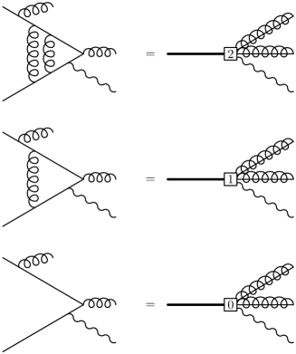
Figure 2: Relevant diagrams in the matching calculation QCD $\rightarrow$ pNRQCD+SCET.

Figure 3: Diagrams which induce an IR scale dependence which cancels against the UV one of the octet shape functions.

The above means that the scale dependence of the leading order contributions of the color-octet currents is of the same order as the NNLO contributions in $\alpha_{\rm s}$ of the color-singlet current, a calculation which is not available. One might, alternatively, attempt to resum logs and use the NLO calculation kramer as the boundary condition. This log resummation is non-trivial. One must take into account the correlation of scales inherent to the non-relativistic system LMR , which in the framework of pNRQCD has been implemented in pinedarg ; currentrg , and combine it with the resummation of Sudakov logs in the framework of SCET luke ; many ; FL0 ; FL (see also hautmann ). Correlations within the various scales of SCET may start playing a role here as well MSS . In any case, it should be clear that by only resumming Sudakov logs, as it has been done so far many , one does not resum all the logs arising in the color octet contributions of heavy quarkonium, at least in the weak coupling regime.

III Application to the $\Upsilon(1S)$

We apply here the results of section II to the $\Upsilon(1S)$. There is good evidence that the $\Upsilon(1S)$ state can be understood as a weak coupling (positronium like) bound state yndurain ; sumino ; hamburg ; pinedahamburg . Hence, ignoring $O\left(\Lambda_{\rm QCD}\right)$ in the shape functions, as we did in section II, should be a reasonable approximation. In the analysis of FL the effects of the octet shape functions were set to zero, so we expect to improve on their results. We plot in Fig. 4 the CLEO data in the end point region cleo , the curve obtained in FL (dashed line) and our curves (solid and dot-dashed lines). Our curves are obtained by adding to the results of FL , which consist of the LL resummation of the singlet contributions only, our (MS) results for the color octet contributions (without LL resummation many ) and setting the scale dependence to $\mu=M\sqrt{1-z}$ (solid line) and to $\mu=2^{\pm 1}M\sqrt{1-z}$ (dot-dashed lines). The first choice is the most reasonable one according to the discussion in the previous section and the last ones are displayed in order to get the flavor of the systematic errors. We have used the following values for the masses and $\alpha_{\rm s}$ in our plots: $m_{b}=4.8$ GeV, $M_{\Upsilon}=9.46$ GeV, $\alpha_{\rm s}\left(\mu_{h}\right)=0.216$, $\alpha_{\rm s}\left(\mu_{s}\right)=0.32$ and $\alpha_{\rm s}\left(\mu_{u}\right)=0.65$. $\mu_{h}\sim m$ stands for the hard scale and is to be used for the $\alpha_{\rm s}$ arising from (3). $\mu_{s}\sim m\alpha_{\rm s}$ stands for the soft scale and is to be used for the $\alpha_{\rm s}$ participating in the bound state dynamics (in $E_{1}$, $I_{S}$, $I_{P}$ and $\psi_{10}({\bf 0})$). $\mu_{u}\sim m\alpha_{\rm s}^{2}$ stands for the ultrasoft scale and is to be used for the $\alpha_{\rm s}$ arising from the coupling of ultrasoft gluons. It turns out that the color octet contribution is numerically enhanced and dominates over the color singlet one in the whole end-point region. In order to compare with the experimental curve, the theoretical result must be convoluted with the experimental efficiency cleo and the overall normalization must be taken as a free parameter. By adjusting our curves to data around $z\sim 0.7$, we obtain an almost perfect agreement in the whole end-point region ($z\in[0.7,1]$) for $\mu=M\sqrt{1-z}$ (solid line). A complete analysis, including systematic errors, is beyond the scope of this paper. It would require either a NNLO matching or a NLO one kramer with NLL resummation of the singlet current. In addition one should estimate what the leading non-perturbative effects are. In any case, it should be clear from our results that the introduction of a gluon mass field is not necessary for the description of the experimental data on the photon spectrum in the end-point region of $\Upsilon(1S)$ radiative decays.

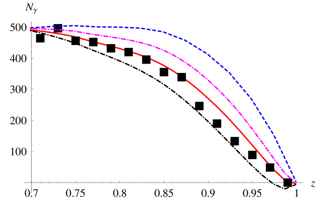
Figure 4: End point region of the photon spectrum in semi-inclusive $\Upsilon$ decay. The points are the CLEO data cleo , the dashed line is the curve obtained in FL and the solid and dot-dashed lines are our results. The solid line is obtained by setting $\mu=M\sqrt{(1-z)}$ (natural choice) and the dot-dashed lines are obtained by setting $\mu=2M\sqrt{1-z}$ and $\mu=2^{-1}M\sqrt{1-z}$.

IV Discussion

We would like to make a few remarks which stem from the details of our calculation. In the existing formulations of SCET, suitable scaling properties are assigned to the various modes. However the standard assignments are violated in our case. The collinear gluons in Fig. 1 scale as $m(\lambda^{2},1,\lambda^{2})$ rather than $m(\lambda^{2},1,\lambda)$ ($\lambda=\sqrt{1-z}$), which is the assigned scaling in bauer ; beneke ; neubert . This indicates that SCET should better be discussed in terms of UV (and IR) cut-offs for the relevant modes, rather than scaling properties. This becomes particularly clear when we analyze the scaling of the ultrasoft gluon in the same diagrams. If $m\alpha_{\rm s}^{2}\sim M(1-z)$, it scales like $m(\lambda^{2},\lambda^{2},\lambda^{2})$ ($\lambda=\alpha_{\rm s}$), which coincides with the standard scaling rules. If, however, $m\alpha_{\rm s}^{4}\sim M(1-z)$, it scales like $m(\lambda^{4},\lambda^{2},\lambda^{3})$, the typical scaling of the recently discovered soft-collinear modes neubert . Either scaling is properly described by the ultrasoft gluons of pNRQCD, since they are defined as the ones having all four momenta much smaller than the soft scale $\sim m\alpha_{\rm s}$ (UV cut-off), which is fulfilled in both cases. However, if one insisted to assign to the ultrasoft gluons a momentum scaling $m(\lambda^{2},\lambda^{2},\lambda^{2})$ and not smaller (i.e. one is introducing an IR cut-off for them), then the situation $m\alpha_{\rm s}^{4}\sim M(1-z)$ would require the introduction of new (ultra)soft-collinear modes scaling like $m(\lambda^{4},\lambda^{2},\lambda^{3})$ with an UV cut-off $\sim m\lambda^{2}$ for the ${+}$ and ${\perp}$ components. Whether it is convenient or not to make such splitting is a matter of debate neubert ; new .

The case $m\alpha_{\rm s}\sim M(1-z)$ has not been discussed. For the color-octet contributions, it requires a calculation in NRQCD, since if one attempts at doing it from Fig. 1 one immediately realizes that the four momentum of the ultrasoft gluon is $\sim m\alpha_{\rm s}$, a region where pNRQCD is not applicable. Hence at NRQCD+SCET_I level (Section II.1) one should calculate a set of diagrams involving a collinear and a soft gluon. The leading order contribution comes from the $S$-wave current only and we have seen it to vanish.

We have refrained ourselves to put forward a Lagrangian for SCET which also holds for heavy quarkonium systems because several issues, like the remarks made above, should be better understood. Clearly, as we have shown in this paper, one cannot simply take over the SCET for heavy-light systems and apply it to heavy quarkonium (for instance, one misses logs which depend on the binding effects). Our analysis also indicates that it may be convenient to rephrase SCET in terms of cut-offs rather than in terms of scaling properties of the various modes as it has been done so far. Then, one would have to account properly for both the suitable cut-offs of pNRQCD and those of SCET.

V Conclusions

Apart from making a few remarks, which we hope will be useful for an eventual construction of a SCET Lagrangian adapted to heavy quarkonium systems, we have calculated the $S$- and $P$-wave octet shape functions in the weak coupling regime. We have also discussed their scale dependence. The addition of these contributions to the ones obtained in FL makes the agreement with data for the end point photon spectrum of inclusive $\Upsilon(1S)$ decays almost perfect. As a by-product the NRQCD matrix elements $\left<\Upsilon(1S)|O_{8}(^{1}S_{0})|\Upsilon(1S)\right>$ and $\left<\Upsilon(1S)|O_{8}(^{3}P_{J})|\Upsilon(1S)\right>$ have also been calculated, in the weak coupling regime, (see Appendix A) and their scale dependence discussed.

Appendix A Calculation of $\Upsilon(1S)$ NRQCD color octet matrix elements

Figure 5: Diagrams which require a ${\cal P}_{1}(^{3}S_{1})$ operator for renormalization. The solid circle stands for either the $O_{8}(^{1}S_{0})$ or $O_{8}(^{3}P_{J})$ operator, the crossed box for either the chromomagnetic (✜ ) or chromoelectric (❶ ) interaction in Fig. 1, the empty box for the octet Coulomb potential, and the thin solid lines for free $Q\bar{Q}$ propagators.

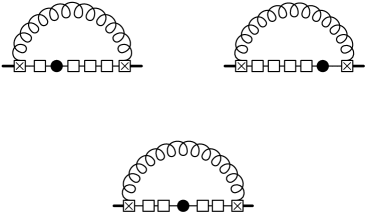
Figure 6: Diagrams which require a $O_{1}(^{3}S_{1})$ operator for renormalization. Symbols are as in Fig. 5.

The calculation in Section II.3 can be easily taken over to provide a calculation of $\left<\Upsilon(1S)\right|$ $\left.O_{8}(\phantom{}^{1}S_{0})|\Upsilon(1S)\right>$ and $\left<\Upsilon(1S)|O_{8}(\phantom{}^{3}P_{J})|\Upsilon(1S)\right>$ assuming that $m\alpha_{\rm s}^{2}\gg\Lambda_{QCD}$ is a reasonable approximation for this system. Indeed, we only have to drop the delta function (which requires a further integration over $k_{+}$) and arrange for the suitable factors in (21) and (22). We obtain

$$\left<\Upsilon(1S)|O_{8}(^{1}S_{0})|\Upsilon(1S)\right>=-2T_{F}^{2}(N_{c}^{2}-1)\int_{0}^{\infty}dk_{+}S_{S}(k_{+})$$

$$\left<\Upsilon(1S)|O_{8}(^{3}P_{J})|\Upsilon(1S)\right>=-{4(2J+1)T_{F}^{2}(N_{c}^{2}-1)\over 3}\int_{0}^{\infty}dk_{+}S_{P1}(k_{+})$$ (25)

where we have used

$$\int_{0}^{\infty}dk_{+}S_{P2}(k_{+})={2\over 3}\int_{0}^{\infty}dk_{+}S_{P1}(k_{+})$$ (26)

The expressions above contain UV divergences which may be regulated in the same way as in Section II.3, namely by calculating the ultrasoft loop in $D$ dimensions. These divergences can be traced back to the diagrams in Fig. 5 and Fig. 6. Indeed, if we expand $I_{S}$ and $I_{P}$ for $z^{\prime}$ large, we obtain

$$I_{S}\sim m\sqrt{\frac{\gamma}{\pi}}\frac{\alpha_{\rm s}N_{c}}{2}\left\{\frac{1}{{z^{\prime}}}+\frac{1}{{z^{\prime}}^{2}}(-1+2\lambda\ln 2)+\frac{1}{{z^{\prime}}^{3}}\left(1-2\lambda+\frac{\lambda^{2}\pi^{2}}{6}\right)+\right.$$

$$\left.+\frac{1}{{z^{\prime}}^{4}}\left(-1+\lambda(2\ln 2+1)+\lambda^{2}(-4\ln 2)+\frac{3}{2}\zeta(3)\lambda^{3}\right)+{\cal O}(\frac{1}{{z^{\prime}}^{5}})\right\}$$ (27)

$$I_{P}\sim\sqrt{\frac{\gamma^{3}}{\pi}}{8\over 3}(2-\lambda)\left\{\frac{1}{2{z^{\prime}}}+\left(-\frac{3}{4}+\lambda\left(-\frac{1}{4}+\ln 2\right)\right)\frac{1}{{z^{\prime}}^{2}}+\right.$$

$$\left.+\left(1-\lambda+\frac{1}{12}(-6+\pi^{2})\lambda^{2}\right)\frac{1}{{z^{\prime}}^{3}}+\frac{1}{4}\left(-5+\lambda+\lambda^{2}(2-8\ln 2)+8\lambda\ln 2+\right.\right.$$

$$\left.\left.+\lambda^{3}\left(-4\ln 2+3\zeta(3)\right)\right)\frac{1}{{z^{\prime}}^{4}}+{\cal O}(\frac{1}{{z^{\prime}}^{5}})\right\}$$ (28)

It is easy to see that only powers of $1/z^{\prime}$ up to order four may give rise to divergences. Moreover, each power of $1/z^{\prime}$ corresponds to one Coulomb exchange. Taking into account the result of the following integral,

$$\int_{0}^{\infty}dk_{+}\int_{0}^{\infty}dx(2k_{+}x)^{-\varepsilon}\frac{1}{{z^{\prime}}^{\alpha}}=2^{1-2\varepsilon}\left(\frac{\gamma^{2}}{m}\right)^{2-2\varepsilon}\frac{\Gamma^{2}(1-\varepsilon)}{\Gamma\left(\frac{\alpha}{2}\right)}\Gamma\left(\frac{\alpha}{2}+2\varepsilon-2\right)$$ (29)

we see that only the $1/{z^{\prime}}^{2}$ and $1/{z^{\prime}}^{4}$ terms produce divergences. The former correspond to diagrams in Fig. 5 and the latter to Fig. 6, which can be renormalized by the operators ${\cal P}_{1}(^{3}S_{1})$ and $O_{1}(^{3}S_{1})$ respectively. It is again important to notice that these divergences are a combined effect of the ultrasoft loop and quantum mechanics perturbation theory (potential loops benekesmirnov ) and hence it may not be clear at first sight if they must be understood as ultrasoft (producing $\log\mu_{u}$ in the notation of Refs. pinedarg ; currentrg ) or potential (producing $\log\mu_{p}$ in the notation of Ref. pinedarg ; currentrg ). In any case, the logarithms they produce depend on the regularization and renormalization scheme used for both ultrasoft and potential loops. Notice that the scheme we use in this work is not the standard one in pNRQCD lambpos ; pinedarg ; hamburg . In the standard scheme the ultrasoft divergences (anomalous dimensions) are identified by dimensionally regulating both ultrasoft and potential loops and subsequently taking $D\rightarrow 4$ in the ultrasoft loop divergences only. If we did this in the present calculation we would obtain no ultrasoft divergence. Hence, in the standard scheme there would be contributions to the potential anomalous dimensions only. The singular pieces in our scheme are displayed below

$$\left.\left<\Upsilon(1S)|O_{8}(^{1}S_{0})|\Upsilon(1S)\right>\right|_{\varepsilon\rightarrow 0}\simeq-{1\over\varepsilon}\left({2\gamma^{2}\over\mu m}\right)^{-2\varepsilon}{1\over 24}C_{F}^{2}N_{c}\alpha_{\rm s}(\mu_{u})\left(C_{f}\alpha_{\rm s}(\mu_{s})\right)^{4}{\gamma^{3}\over\pi^{2}}\Bigg{(}2+$$

$$\left.+\lambda\left[-7-4\log 2\right]+\lambda^{2}\left[4+8\log 2+4\log^{2}2+{\pi^{2}\over 3}\right]+\lambda^{3}\left[-4\log^{2}2-{\pi^{2}\over 3}-{3\over 2}\zeta(3)\right]\right)$$

$$\left.\left<\Upsilon(1S)|O_{8}(^{3}P_{J})|\Upsilon(1S)\right>\right|_{\varepsilon\rightarrow 0}\simeq-(2J+1){1\over\varepsilon}\left({2\gamma^{2}\over\mu m}\right)^{-2\varepsilon}{4\over 27}C_{f}\alpha_{\rm s}(\mu_{u})(C_{f}\alpha_{\rm s}(\mu_{s}))^{2}{\gamma^{5}\over\pi^{2}}\times$$

$$\times(2-\lambda)\left(-4++\lambda\left[{47\over 12}+5\log 2\right]+\lambda^{2}\left[{5\over 6}-{2\pi^{2}\over 9}-{8\over 3}\log 2-{8\over 3}\log^{2}2\right]+\right.$$

$$\left.+\lambda^{3}\left[-{7\over 12}+{\pi^{2}\over 9}-{5\over 3}\log 2+{4\over 3}\log^{2}2+{3\over 4}\zeta(3)\right]\right)$$ (30)

References

- (1) M. J. Dugan and B. Grinstein, Phys. Lett. B 255 (1991) 583.
- (2) C. W. Bauer, S. Fleming and M. E. Luke, Phys. Rev. D 63 (2001) 014006 [arXiv:hep-ph/0005275].
- (3) C. W. Bauer, S. Fleming, D. Pirjol and I. W. Stewart, Phys. Rev. D 63 (2001) 114020 [arXiv:hep-ph/0011336]; C. W. Bauer and I. W. Stewart, Phys. Lett. B 516 (2001) 134 [arXiv:hep-ph/0107001]; C. W. Bauer, D. Pirjol and I. W. Stewart, Phys. Rev. D 65 (2002) 054022 [arXiv:hep-ph/0109045]; Phys. Rev. D 66 (2002) 054005 [arXiv:hep-ph/0205289]; Phys. Rev. D 68 (2003) 034021 [arXiv:hep-ph/0303156]; D. Pirjol and I. W. Stewart, Phys. Rev. D 67 (2003) 094005 [arXiv:hep-ph/0211251].
- (4) M. Beneke, A. P. Chapovsky, M. Diehl and T. Feldmann, Nucl. Phys. B 643 (2002) 431 [arXiv:hep-ph/0206152]; M. Beneke and T. Feldmann, Phys. Lett. B 553 (2003) 267 [arXiv:hep-ph/0211358].
- (5) R. J. Hill and M. Neubert, Nucl. Phys. B 657 (2003) 229 [arXiv:hep-ph/0211018]; T. Becher, R. J. Hill and M. Neubert, arXiv:hep-ph/0308122; T. Becher, R. J. Hill, B. O. Lange and M. Neubert, arXiv:hep-ph/0309227.
- (6) M. Beneke, http://wwwteor.mi.infn.it/ brambill/school.html; M. Neubert, ibid.
- (7) C. W. Bauer, S. Fleming, D. Pirjol, I. Z. Rothstein and I. W. Stewart, Phys. Rev. D 66 (2002) 014017 [arXiv:hep-ph/0202088].
- (8) M. Beneke and T. Feldmann, arXiv:hep-ph/0311335; B. O. Lange and M. Neubert, arXiv:hep-ph/0311345; C. W. Bauer, M. P. Dorsten and M. P. Salem, arXiv:hep-ph/0312302; J. Chay and C. Kim, arXiv:hep-ph/0401089.
- (9) C. W. Bauer, C. W. Chiang, S. Fleming, A. K. Leibovich and I. Low, Phys. Rev. D 64 (2001) 114014 [arXiv:hep-ph/0106316].
- (10) S. Fleming and A. K. Leibovich, Phys. Rev. Lett. 90 (2003) 032001 [arXiv:hep-ph/0211303].
- (11) S. Fleming and A. K. Leibovich, Phys. Rev. D 67 (2003) 074035 [arXiv:hep-ph/0212094].
- (12) B. Nemati et al. [CLEO Collaboration], Phys. Rev. D 55 (1997) 5273 [arXiv:hep-ex/9611020].
- (13) S. J. Brodsky, D. G. Coyne, T. A. DeGrand and R. R. Horgan, Phys. Lett. B 73 (1978) 203; D. M. Photiadis, Phys. Lett. B 164 (1985) 160; S. Wolf, Phys. Rev. D 63 (2001) 074020 [arXiv:hep-ph/0010217].
- (14) A. L. Kagan and M. Neubert, Eur. Phys. J. C 7 (1999) 5 [arXiv:hep-ph/9805303]; F. De Fazio and M. Neubert, JHEP 9906 (1999) 017 [arXiv:hep-ph/9905351].
- (15) S. Titard and F. J. Yndurain, Phys. Rev. D 49 (1994) 6007 [arXiv:hep-ph/9310236]; Phys. Rev. D 51 (1995) 6348 [arXiv:hep-ph/9403400]; Phys. Lett. B 351 (1995) 541 [arXiv:hep-ph/9501338]; A. Pineda and F. J. Yndurain, Phys. Rev. D 58 (1998) 094022 [arXiv:hep-ph/9711287]; Phys. Rev. D 61 (2000) 077505 [arXiv:hep-ph/9812371]; A. Pineda, JHEP 0106 (2001) 022 [arXiv:hep-ph/0105008].
- (16) N. Brambilla, Y. Sumino and A. Vairo, Phys. Lett. B 513 (2001) 381 [arXiv:hep-ph/0101305]; Phys. Rev. D 65 (2002) 034001 [arXiv:hep-ph/0108084]; S. Recksiegel and Y. Sumino, Phys. Rev. D 67 (2003) 014004 [arXiv:hep-ph/0207005].
- (17) B. A. Kniehl, A. A. Penin, V. A. Smirnov and M. Steinhauser, Nucl. Phys. B 635 (2002) 357 [arXiv:hep-ph/0203166]; A. A. Penin and M. Steinhauser, Phys. Lett. B 538 (2002) 335 [arXiv:hep-ph/0204290].
- (18) B. A. Kniehl, A. A. Penin, A. Pineda, V. A. Smirnov and M. Steinhauser, arXiv:hep-ph/0312086.
- (19) B. A. Kniehl, A. A. Penin, M. Steinhauser and V. A. Smirnov, Phys. Rev. Lett. 90 (2003) 212001 [arXiv:hep-ph/0210161].
- (20) G. T. Bodwin, E. Braaten and G. P. Lepage, Phys. Rev. D 51 (1995) 1125 [Erratum-ibid. D 55 (1997) 5853] [arXiv:hep-ph/9407339].
- (21) A. Pineda and J. Soto, Nucl. Phys. Proc. Suppl. 64 (1998) 428 [arXiv:hep-ph/9707481]; N. Brambilla, A. Pineda, J. Soto and A. Vairo, Nucl. Phys. B 566 (2000) 275 [arXiv:hep-ph/9907240].
- (22) I. Z. Rothstein and M. B. Wise, Phys. Lett. B 402 (1997) 346 [arXiv:hep-ph/9701404].
- (23) F. Maltoni and A. Petrelli, Phys. Rev. D 59 (1999) 074006 [arXiv:hep-ph/9806455].
- (24) M. Kramer, Phys. Rev. D 60 (1999) 111503 [arXiv:hep-ph/9904416].
- (25) N. Brambilla, D. Eiras, A. Pineda, J. Soto and A. Vairo, Phys. Rev. D 67 (2003) 034018 [arXiv:hep-ph/0208019].
- (26) M. Beneke, G. A. Schuler and S. Wolf, Phys. Rev. D 62 (2000) 034004 [arXiv:hep-ph/0001062].
- (27) M. E. Luke, A. V. Manohar and I. Z. Rothstein, Phys. Rev. D 61 (2000) 074025 [arXiv:hep-ph/9910209].
- (28) A. Pineda, Phys. Rev. D 65 (2002) 074007 [arXiv:hep-ph/0109117]; A. Pineda, Phys. Rev. A 66 (2002) 062108 [arXiv:hep-ph/0204213].
- (29) A. Pineda, Phys. Rev. D 66 (2002) 054022 [arXiv:hep-ph/0110216].
- (30) F. Hautmann, Nucl. Phys. B 604 (2001) 391 [arXiv:hep-ph/0102336].
- (31) A. V. Manohar, J. Soto and I. W. Stewart, Phys. Lett. B 486 (2000) 400 [arXiv:hep-ph/0006096].
- (32) J. H. Field, Phys. Rev. D 66 (2002) 013013 [arXiv:hep-ph/0101158].
- (33) M. Beneke and V. A. Smirnov, Nucl. Phys. B 522 (1998) 321 [arXiv:hep-ph/9711391].
- (34) A. Pineda and J. Soto, Phys. Lett. B 420 (1998) 391 [arXiv:hep-ph/9711292]; A. Pineda and J. Soto, Phys. Rev. D 59 (1999) 016005 [arXiv:hep-ph/9805424].