Three-generation flavor transitions and decays
of supernova relic neutrinos

Abstract

If neutrinos have mass, they can also decay. Decay lifetimes of cosmological interest can be probed, in principle, through the detection of the redshifted, diffuse neutrino flux produced by all past supernovae—the so-called supernova relic neutrino (SRN) flux. In this work, we solve the SRN kinetic equations in the general case of three-generation flavor transitions followed by invisible (nonradiative) two-body decays. We then use the general solution to calculate observable SRN spectra in some representative decay scenarios. It is shown that, in the presence of decay, the SRN event rate can basically span the whole range below the current experimental upper bound—a range accessible to future experimental projects. Radiative SRN decays are also briefly discussed.

I Introduction

In the last few years, compelling evidence has emerged in favor of neutrino masses and mixings (see, e.g., Revi for recent reviews). Within a three-generation framework, the known flavor eigenstates of neutrinos $\nu_{\alpha}$ and antineutrinos $\bar{\nu}_{\alpha}$ $(\alpha=e,\mu,\tau)$ must then be considered as linear superpositions of mass eigenstates $\nu_{i}$ ($i=1,2,3$),

$${\stackrel{{\scriptstyle{}_{(-)}}}{{\nu}}\!\!}_{\alpha}=\sum_{i}U_{\alpha i}{\stackrel{{\scriptstyle{}_{(-)}}}{{\nu}}\!\!}_{i}\ ,$$ (1)

where the mixing matrix $U_{\alpha i}$ (assumed here to be real for simplicity) can be expressed in terms of three mixing angles $(\theta_{12},\theta_{13},\theta_{23})$ in the standard parametrization Hagi . The $\nu_{i}$ squared mass spectrum can be cast in the form

$$(m^{2}_{1},m^{2}_{2},m^{2}_{3})=M^{2}+\left(-\frac{\delta m^{2}}{2},+\frac{\delta m^{2}}{2},\pm\Delta m^{2}\right)\ ,$$ (2)

where $\delta m^{2}$ and $\Delta m^{2}$ govern the two independent $\nu$ oscillation frequencies, while $M^{2}$ fixes the absolute $\nu$ mass scale. Current neutrino oscillation data (see, e.g., Sola ; Atmo ) provide the best-fit values:

$$\delta m^{2} \simeq 7.2\times 10^{-5}\mathrm{\ eV}^{2}\ ,$$ (3)

$$|\pm\Delta m^{2}| \simeq 2.0\times 10^{-3}\mathrm{\ eV}^{2}\ ,$$ (4)

$$\sin^{2}\theta_{12} \simeq 0.29\ ,$$ (5)

$$\sin^{2}\theta_{23} \simeq 0.50\ ,$$ (6)

and the upper bound (at $3\sigma$) Atmo

$$\sin^{2}\theta_{13}<0.067\ .$$ (7)

The sign of $\Delta m^{2}$ is currently unknown, while $M^{2}$ is bounded from above by laboratory and astrophysical constraints ($\sqrt{M^{2}}\lesssim{\mathrm{few}}\times 10^{-1}$ eV Revi ).

In general, massive neutrinos can not only mix, but also decay (see, e.g., the reviews in Dolg ; Pakv ; Gelm ). Neutrino decay has been invoked in the past, e.g., to solve the solar neutrino problem or the atmospheric neutrino anomaly (see Pak2 and references therein). These and other neutrino decay solutions have not been experimentally validated so far, implying that the decay lifetimes ($\tau_{i}$ in the rest frame) must be sufficiently long to leave unperturbed the current neutrino phenomenology. Roughly speaking, this can be achieved by imposing $\tau_{i}E/m_{i}L\gg 1$ in the laboratory frame, where $L$ and $E$ are the neutrino pathlength and energy, respectively. Such arguments, properly refined and applied to solar neutrinos [$L/E\sim O(10^{7})$ km/MeV], lead to a safe lower bound Bell

$$\frac{\tau_{i}}{m_{i}}\gtrsim 5\times 10^{-4}\mathrm{\ s/eV}\ .$$ (8)

Similarly, from the supernova (SN) 1987A neutrino events [$L/E\sim O(10^{16})$ km/MeV] one might naively guess a much stronger lower bound,

$$\frac{\tau_{i}}{m_{i}}\gtrsim O(10^{5})\mathrm{\ s/eV}\ ,$$ (9)

which, however, does not hold for relatively large values of the mixing angle $\theta_{12}$ SN87 , as those implied by current data in Eq. (5) (see also the comment at the end of Sec. IV C). On the other hand, for neutrino decay effects to be observable in our universe, it must be roughly $\tau_{i}E/m_{i}\lesssim 1/H_{0}$, where $H_{0}$ is the Hubble constant; by setting $H_{0}=70\;\mathrm{km}\,\mathrm{s}^{-1}\,\mathrm{Mpc}^{-1}$ and taking $E\sim O(10)$ MeV (i.e., in the energy range probed by supernova neutrinos), a rough upper bound for the “neutrino decay observability” is obtained,

$$\frac{\tau_{i}}{m_{i}}\lesssim O(10^{11})\mathrm{\ s/eV}\ .$$ (10)

The comparison of Eqs. (8) and (10) implies that many decades in $\tau_{i}/m_{i}$ are still open to experimental and theoretical investigations.

The exploration of relatively long neutrino lifetimes, and of the associated decay effects, can be effectively pursued through astrophysical and cosmological observations. For instance, evidence for neutrino decay might be signaled by an anomalous flavor composition of high-energy astrophysical neutrinos Be03 . Neutrino decay might also profoundly alter the flux of supernova relic neutrinos (SRN) and possibly push it close to the current experimental SRN upper bounds SKSN ; Male , as recently pointed out in Ref. Ando . Given the promising prospects for detecting SRN signals in the Super-Kamiokande (SK) water Cherenkov detector (if doped with Gd GADZ ) or in planned larger detectors such as the Underground Nucleon Decay and Neutrino Observatory (UNO) UNNO or Hyper-Kamiokande Hype , we think that the interesting idea of probing neutrino decay through SRN data Ando appears as an opportunity which, although challenging, deserves further studies.

On the basis of the previous motivations, in this work we aim at providing a general framework, as well as specific examples, for the calculation of nonradiative two-body decays of SRN,

$$\nu_{i}\to{\stackrel{{\scriptstyle{}_{(-)}}}{{\nu}}\!\!}_{j}+X\$$ (11)

(and for analogous antineutrino decays), where $X$ is a (pseudo)scalar particle, e.g., a Majoron Gelm . After considering the “standard” case of $3\nu$ flavor transitions without decay in Sec. II, we discuss in Sec. III the more general case of $3\nu$ transitions followed by decays, and give the explicit solution of the neutrino kinetic equations for generic decay parameters. Specific numerical examples (inspired by neutrino-Majoron decay models) are given in Sec. IV, in order to show representative SRN event rates and energy spectra in the presence of decay. Conclusions and prospects for future work are given in Sec. V.

A final remark is in order. In this paper, we focus on invisible two-body decays [Eq. (11)] since they can be tested, in principle, by future SRN data. Invisible decays into three neutrinos are not considered here, also because the typical final-state neutrino energy would generally be too low to be probed by SRN observations. Radiative two-body neutrino decays, instead, do not suffer of such “low-energy” $\nu$ detection problem, but are however severely constrained by the current astrophysical $\gamma$-ray phenomenology. A brief discussion of the photon background from hypothetical SRN radiative decays is given in Appendix A. Appendix B finally deals with some subdominant $3\nu$ oscillation effects in the atmospheric neutrino background, which are often overlooked in SRN searches.

II Three-neutrino flavor transitions without decay

In this Section we consider the standard case of flavor transitions among three stable neutrinos. Although the no-decay case for SRN has already been treated in previous works (see, e.g., An03 ; AnSa ; Fuku ; Ka03 ; An04 for recent contributions), we prefer to discuss its calculations in some detail, both to make the paper self-consistent, and to better appreciate the differences with the case of unstable neutrinos. In this Section we also define the notation, as well as our default choices and approximations for several inputs (from cosmology and astrophysics, neutrino oscillation data, and supernova simulations) needed to compute the SRN signal. The same inputs will be used in the presence of $\nu$ decay (Sec. IV).

We do not address here the problem of the uncertainties affecting these—and other equally admissible—input choices, being mainly interested to highlight the additional effects of neutrino decay (as compared with the standard case). Careful considerations about central values and uncertainties of the various inputs will be necessary, however, when supernova relic neutrinos will be eventually detected by experiments and used to constrain models, with or without neutrino decay (see An04 for a recent approach using simulated data).

Finally, we remind that three-flavor oscillations affect not only the signal in SRN searches, but also the background. We discuss in Appendix B some subtle $3\nu$ effects which are often neglected in calculating the atmospheric neutrino background rate.

II.1 Input from cosmology and astrophysics

The local (redshift $z=0$) number density of mass eigenstates $\nu_{i}$ per unit of energy, coming from all past core-collapse supernovae, is given by (see, e.g., An03 ):

$$n_{\nu_{i}}(E)=\int_{0}^{\infty}{dz\,H^{-1}(z)\,R_{\mathrm{SN}}(z)\,Y_{\nu_{i}}(E(1+z))}\ ,$$ (12)

where $R_{\mathrm{SN}}(z)$ is the supernova formation rate (per unit of time and of comoving volume at redshift $z$), $Y_{\nu_{i}}(q)$ is the average yield of $\nu_{i}$ for a typical supernova [per unit of initial, unredshifted energy $q=E(1+z)$], and $H(z)$ is the Hubble constant at redshift $z$ which, in standard notation Hagi , reads

$$H(z)=H_{0}[(1+z)^{2}(1+\Omega_{M}z)-\Omega_{\Lambda}z(2+z)]^{\frac{1}{2}}\ .$$ (13)

Since supernova relic neutrinos are ultrarelativistic ($v\simeq c$), the above number density per unit of energy $n_{\nu_{i}}(E)$ can be identified, in natural units ($c=1$), with the local relic $\nu_{i}$ flux per unit of time, area, and energy.

We assume, following An03 ; Fuku , that the function $R_{\mathrm{SN}}$ is given by

$$R_{\mathrm{SN}}(z)=0.0122\,R_{\mathrm{SF}}(z)/M_{\odot}\ ,$$ (14)

where the star formation rate $R_{\mathrm{SF}}$ is parametrized as Mada

$$R_{\mathrm{SF}}(z)=0.3\,h_{65}\,\frac{\exp(3.4z)}{45+\exp(3.8z)}\;\;M_{\odot}\mathrm{yr}^{-1}\mathrm{Mpc}^{-3}$$ (15)

for $z<5$ (and $R_{\mathrm{SF}}=0$ otherwise An03 ), with $h_{65}=H_{0}/65\;\mathrm{km}\,\mathrm{s}^{-1}\,\mathrm{Mpc}^{-1}$. (Other choices are also possible for $R_{\mathrm{SF}}$; see, e.g., Ka03 .)

The above expression for $R_{\mathrm{SF}}$ actually holds for an Einstein-de Sitter cosmology $(\Omega_{M},\Omega_{\Lambda})=(1,0)$. For a different cosmology one has to apply a correction factor An03

$$R_{\mathrm{SF}}\to R_{\mathrm{SF}}\frac{[(1+z)^{2}(1+\Omega_{M}z)-\Omega_{\Lambda}z(2+z)]^{\frac{1}{2}}}{(1+z)^{\frac{3}{2}}}\ ,$$ (16)

which cancels the dependence of $n_{\nu_{i}}$ upon $(\Omega_{M},\Omega_{\Lambda})$ in Eq. (12). This cancellation does not apply in the presence of neutrino decay (see Sec. III B). When needed, we shall then fix $\Omega_{M}=0.3$, $\Omega_{\Lambda}=0.7$, and $h_{65}=1.077$ (i.e., $H_{0}=70\;\mathrm{km}\,\mathrm{s}^{-1}\,\mathrm{Mpc}^{-1}$), consistently with recent determinations of cosmological parameters SDSS .

II.2 Input from neutrino oscillation phenomenology

The smallness of the $\delta m^{2}/\Delta m^{2}$ ratio [see Eqs. (3) and (4)] and of $\sin^{2}\theta_{13}$ [see Eq. (7)] lead to the approximate decoupling of the supernova $3\nu$ dynamics into “high” ($H$) and “low” ($L$) $2\nu$ subsystems, governed by $(k_{H},\sin^{2}\theta_{13})$ and $(k_{L},\sin^{2}\theta_{12})$, respectively, where $k_{H}=\pm\Delta m^{2}/2E$ and $k_{L}=\delta m^{2}/2E$ are the two independent neutrino wavenumbers (see, e.g., SNan and references therein). Matter effects Matt are governed by the potential $V=\pm\sqrt{2}\,G_{F}\,N_{e}(x)$, where $N_{e}(x)$ is the electron density at radius $x$ (roughly falling as $x^{-3}$ outside the supernova neutrinosphere, up to shock-wave effects Shoc ), and the plus (minus) sign refers to neutrinos (antineutrinos). The four cases corresponding to $\mathrm{sign}(\Delta m^{2})=\pm 1$ (normal or inverted hierarchy) and $\mathrm{sign}(V)=\pm 1$ (neutrinos or antineutrinos) lead, in general, to different physics.

In supernova neutrino oscillations, it is customary to average out unobservable interference phases from the beginning, and to work directly in terms of level crossing probabilities $P_{ij}$ KuPa . At the exit from the supernova, the yields of neutrino mass eigenstates $Y_{\nu_{i}}$ are then given by

$$Y_{\nu_{i}}=\sum_{\alpha,j}P_{ij}\,|U^{m}_{\alpha j}|^{2}\,Y_{\nu_{\alpha}}\$$ (17)

(and similarly for antineutrinos), where $U^{m}_{\alpha j}$ and $Y_{\nu_{\alpha}}$ are, respectively, the mixing matrix elements in matter and the neutrino flavor yields at the neutrinosphere.

The usual assumption $Y_{\nu_{\mu}}=Y_{\nu_{\tau}}=Y_{\bar{\nu}_{\mu}}=Y_{\bar{\nu}_{\tau}}\equiv Y_{\nu_{x}}$ implies that the inner matrix product in Eq. (17) depends only on $Y_{\nu_{x}}$, $Y_{\nu_{e}}$ for neutrinos ($Y_{\nu_{x}}$, $Y_{\bar{\nu}_{e}}$ for antineutrinos), and on the squared mixing matrix elements $|U^{m}_{ei}|^{2}$. Such elements are given by

$$(|U^{m}_{e1}|^{2},|U^{m}_{e2}|^{2},|U^{m}_{e3}|^{2})=(\cos^{2}\theta_{13}^{m}\,\cos^{2}\theta_{12}^{m},\,\cos^{2}\theta_{13}^{m}\,\sin^{2}\theta_{12}^{m},\,\sin^{2}\theta_{13}^{m})\ ,$$ (18)

where

$$\cos 2\theta_{13}^{m} \simeq \frac{\cos 2\theta_{13}-V/k_{H}}{\sqrt{(\cos 2\theta_{13}-V/k_{H})^{2}+\sin^{2}2\theta_{13}}}\simeq-\mathrm{sign}(V)\mathrm{sign}(\Delta m^{2})\ ,$$ (19)

$$\cos 2\theta_{12}^{m} \simeq \frac{\cos 2\theta_{12}-V/k_{L}}{\sqrt{(\cos 2\theta_{12}-V/k_{L})^{2}+\sin^{2}2\theta_{12}}}\simeq-\mathrm{sign}(V)\ ,$$ (20)

and we have used the fact that $|V/k_{H,L}|\gg 1$ at the neutrinosphere.

A further simplification of Eq. (17) comes from the adiabaticity of the $1\leftrightarrow 2$ level crossing in the $L$ subsystem [$P_{L}\simeq 0$ for the mass-mixing values in Eqs. (3) and (5)]. The matrix $P_{ij}$ has then (at most) one nontrivial $2\times 2$ submatrix with indices $(k,l)$ and off-diagonal entry $P_{H}$, where $P_{H}$ is the $k\leftrightarrow l$ crossing probability in the $H$ subsystem (equal for $\nu$ and $\bar{\nu}$ SNan ). The final results for the yield of the $i$-th mass eigenstate at the exit from the supernova are collected in Table I.

Table 1: Relevant mixing matrix elements and supernova neutrino yields in the four possible $3\nu$ scenarios. The $k\leftrightarrow l$ level crossing in the $H$ system (if any) is reported in the 5th column. See the text for details.

Scenario	$|U^{m}_{e1}|^{2}$	$|U^{m}_{e2}|^{2}$	$|U^{m}_{e3}|^{2}$	$k\leftrightarrow l$	Yield of $i$-th $\nu$ state
					$Y_{\nu_{1}}=Y_{\nu_{x}}$
$\nu$, normal hierarchy	0	0	1	$3\leftrightarrow 2$	$Y_{\nu_{2}}=(1-P_{H})Y_{\nu_{x}}+P_{H}Y_{\nu_{e}}$
					$Y_{\nu_{3}}=P_{H}Y_{\nu_{x}}+(1-P_{H})Y_{\nu_{e}}$
					$Y_{\bar{\nu}_{1}}=Y_{\bar{\nu}_{e}}$
$\bar{\nu}$, normal hierarchy	1	0	0	—	$Y_{\bar{\nu}_{2}}=Y_{\nu_{x}}$
					$Y_{\bar{\nu}_{3}}=Y_{\nu_{x}}$
					$Y_{\nu_{1}}=Y_{\nu_{x}}$
$\nu$, inverted hierarchy	0	1	0	—	$Y_{\nu_{2}}=Y_{\nu_{e}}$
					$Y_{\nu_{3}}=Y_{\nu_{x}}$
					$Y_{\bar{\nu}_{1}}=(1-P_{H})Y_{\nu_{x}}+P_{H}Y_{\bar{\nu}_{e}}$
$\bar{\nu}$, inverted hierarchy	0	0	1	$3\leftrightarrow 1$	$Y_{\bar{\nu}_{2}}=Y_{\nu_{x}}$
					$Y_{\bar{\nu}_{3}}=P_{H}Y_{\nu_{x}}+(1-P_{H})Y_{\bar{\nu}_{e}}$

In general, the crossing probability $P_{H}$ depends on the $\nu$ potential profile $V(x)$ (see, e.g., SNan ). This dependence vanishes in the limiting cases of adiabatic transitions ($P_{H}\simeq 0$) and strongly nonadiabatic transitions ($P_{H}\simeq 1$), which correspond roughly to $\sin^{2}\theta_{13}\gg 10^{-4}$ and $\sin^{2}\theta_{13}\ll 10^{-5}$, respectively (see, e.g., Luna ). In our numerical examples, we shall consider for simplicity only the two limiting cases,

$$P_{H}=0\mathrm{\ or\ }1\ .$$ (21)

For our purposes, we can also neglect the secondary corrections due to Earth matter crossing SNan ; Luna for arrival neutrino directions below the horizon. In this approximation, the number density of SRN in the flavor basis is simply given by

$$n_{\nu_{\alpha}}(E)=\sum_{i}|U_{\alpha i}|^{2}n_{\nu_{i}}(E)\ ,$$ (22)

and similarly for antineutrinos. Finally, in the phenomenologically interesting case of supernova relic $\bar{\nu}_{e}$ one gets, up to negligible terms of $O(\sin^{2}{\theta_{13}})$,

$$n_{\bar{\nu}_{e}}(E)\simeq\cos^{2}\theta_{12}\,n_{\bar{\nu}_{1}}(E)+\sin^{2}\theta_{12}\,n_{\bar{\nu}_{2}}(E)\ ,$$ (23)

where $\sin^{2}\theta_{12}$ is taken from Eq. (5).

II.3 Input from supernova simulations

Concerning the three relevant $\nu$ flavor yields at the neutrinosphere $Y_{\nu}$ ($\nu=\nu_{e},\bar{\nu}_{e},\nu_{x}$), we assume for simplicity equipartition of the total binding energy $E_{b}$ (taken equal to $3\times 10^{53}$ erg) among all flavors,

$$Y_{\nu}(E)=\frac{E_{b}}{6\langle E\rangle_{\nu}}\,\varphi(E;\langle E\rangle_{\nu},\alpha)\ ,$$ (24)

where $\varphi(E)$ is the normalized neutrino spectrum ($\int dE\varphi=1$), $\langle E\rangle_{\nu}$ is the average $\nu$ energy, and $\alpha$ is a spectral parameter. A useful spectral parametrization is given in Ref. Spec :

$$\varphi(E)=\frac{(\alpha+1)^{(\alpha+1)}}{\Gamma(\alpha+1)}\left(\frac{E}{\langle E\rangle_{\nu}}\right)^{\alpha}\frac{e^{-(\alpha+1)E/\langle E\rangle_{\nu}}}{\langle E\rangle_{\nu}}\ ,$$ (25)

where $\Gamma$ is the Euler gamma function. From the admissible parameter ranges in Ref. Spec , we pick up the following values:

$$(\langle E\rangle_{\nu_{e}},\langle E\rangle_{\bar{\nu}_{e}},\langle E\rangle_{\nu_{x}})=(12,15,18)\ \mathrm{MeV}\ ,$$ (26)

$$\alpha=3\ .$$ (27)

Figure 1 shows the functions $Y_{\nu_{e}}(E)$, $Y_{\bar{\nu}_{e}}(E)$, and $Y_{\nu_{x}}(E)$, which follow from the previous assumptions. We emphasize that such assumptions are not meant to provide “reference” or “best” neutrino spectra, but just a reasonable input for our numerical computations and for the comparison of results with and without decay.

Figure 1: Supernova neutrino yields of $\nu_{e}$, $\bar{\nu}_{e}$, and $\nu_{x}$ (curves labelled by $Y_{\nu_{e}}$, $Y_{\bar{\nu}_{e}}$, $Y_{\nu_{x}}$, respectively), as defined through Eqs. (24)–(27).

II.4 Results for supernova relic $\bar{\nu}_{e}$ fluxes and positron spectra (no decay)

Supernova relic $\bar{\nu}_{e}$’s can produce observable signals (positrons) through the reaction:

$$\bar{\nu}_{e}+p\to n+e^{+}\ .$$ (28)

For our purposes, the cross section for this process can be approximated at zeroth order Xsec , with $E_{e^{+}}=E_{\nu}-1.293$ MeV, where $E_{e^{+}}$ is the total (true) positron energy. We will generically refer to “water targets” but not to specific detectors; therefore, we will not include experiment-dependent details such as the difference between true and measured positron energy (i.e., the detector resolution function), or the detector efficiency function.

Figure 2: Supernova relic $\bar{\nu}_{e}$ spectrum (middle panel), and associated positron spectrum from $\bar{\nu}_{e}+p\to n+e^{+}$ (right panel), in the presence of $3\nu$ flavor transitions without decay. The spectra depend on the mass hierarchy (left panel), which can be either normal (NH) or inverted (IH). In the latter case, there is a further dependence on the crossing probability $P_{H}$. The representative cases $P_{H}=0$ (“large $\theta_{13}$”) and $P_{H}=1$ (“small $\theta_{13}$”) are shown.

Figure 2 shows our SRN flux calculations for no decay, in both cases of normal hierarchy (NH) and inverted hierarchy (IH), as reported in the left panel. The middle panel refers to the absolute supernova relic $\bar{\nu}_{e}$ fluxes [Eq. (23)] in units of $\bar{\nu}_{e}$/MeV/cm²/s, as a function of neutrino energy. The right panel refers to the absolute positron event rate per MeV and per kton-year (kTy) in water, as a function of the true positron energy. In the case of normal hierarchy (solid curves), the $\bar{\nu}_{e}$ and positron spectra do not depend on the crossing probability $P_{H}$ (see Table I). This case is indistinguishable from the case of inverted hierarchy with $P_{H}=1$ AnSa . In both such cases (NH with any $P_{H}$, or IH with $P_{H}=1$) it is

$$n_{\bar{\nu}_{e}}(E)=\int_{0}^{\infty}{dz\,H^{-1}(z)\,R_{\mathrm{SN}}(z)\,[\cos^{2}\theta_{12}\,Y_{\bar{\nu}_{e}}(E(1+z))+\sin^{2}\theta_{12}Y_{\nu_{x}}(E(1+z))]}\ .$$ (29)

In the case of inverted hierarchy with $P_{H}=0$ (dashed curves in Fig. 2), the supernova relic $\bar{\nu}_{e}$ spectrum depends only on $Y_{\nu_{x}}$,

$$n_{\bar{\nu}_{e}}(E)=\int_{0}^{\infty}{dz\,H^{-1}(z)\,R_{\mathrm{SN}}(z)\,Y_{\nu_{x}}(E(1+z))}\ ,$$ (30)

and is thus peaked at somewhat higher energy [see Eq. (24) and Fig. 1].

The results in Fig. 2 are in agreement with previous absolute estimates of the neutrino and positron spectra in water-Cherenkov detectors (see, e.g., AnSa ), modulo different choices for (some of) the inputs of SRN calculations. As we shall see, such results can be profoundly modified by neutrino decay.

III Three-neutrino flavor transitions and decays

In this Section we discuss and solve the neutrino kinetic equations in the general case of $3\nu$ flavor transitions plus decay. We consider generic rest-frame (anti)neutrino lifetimes $\tau_{i}$ and associated decay widths,

$$\tau_{i}^{-1}=\Gamma_{i}=\sum_{m_{j}<m_{i}}\Gamma(\nu_{i}\to\nu_{j})\ +\Gamma(\nu_{i}\to\bar{\nu}_{j})\ .$$ (31)

Also, in this Section we do not set restrictions on branching ratios

$$B(\nu_{i}\to\nu_{j})=\Gamma(\nu_{i}\to\nu_{j})/\Gamma_{i}\ ,$$ (32)

and on neutrino decay energy spectra

$$\psi_{\nu_{i}\to\nu_{j}}(E_{i},E_{j})=\mathrm{Prob}[\nu_{i}(E_{i})\to\nu_{j}(E_{j})]\$$ (33)

(normalized to unity, $\int dE_{j}\,\psi(E_{i},E_{j})=1$).

Notice that, for $\tau_{i}/m_{i}$ values above the bound in Eq. (8), supernova relic $\nu$ flavor transitions occur in matter (and become incoherent) well before neutrino decay losses become significant, so that hypothetical interference effects between the two phenomena Lind can be neglected. For our purposes, flavor transitions inside the supernova can thus be taken as decoupled from the subsequent (incoherent) propagation and decay of mass eigenstates in vacuum.

An important remark is in order. In this work we consider only vacuum neutrino decays. It is possible, however, to construct models where fast invisible decays can be triggered by matter effects Bere ; GLam at the very high densities characterizing the supernova neutrinosphere, even in the absence of vacuum decays (e.g, for diagonal neutrino-Majoron couplings; see, e.g. Kach ). In such scenarios, matter-induced decays might thus occur before flavor transitions in supernovae, leading to a phenomenology rather different from the one considered in this paper (and subject to model-dependent constraints from supernova energetics Kach ; Smir ; Choi ; Toma ; Farz ). We emphasize that the results discussed in the following sections are generally applicable to vacuum neutrino decays occurring after flavor transitions, while possible matter-induced fast decays are beyond the scope of this work.

III.1 Kinetic equations

In the presence of $\nu$ decay, the local ($z=0$) SRN number density per unit energy $n_{\nu_{i}}(E)$ depends on the history of all past ($z>0$) decays having the $\nu_{i}$ as initial or final mass state. The functions $n_{\nu_{i}}(E,z)$ (number of $\nu_{i}$ per unit of comoving volume and of energy at redshift $z$) can be obtained through a direct integration of the neutrino kinetic equations, as described below.

The generic form of the kinetic equations for the phase-space distribution function $f$ is

$${\cal L}[f]={\cal C}[f]\ ,$$ (34)

where $\cal L$ is the Liouville operator and $\cal C$ is the collision operator, embedding creation and destruction terms for the particle described by $f$ (see, e.g., Dolg ; Kolb ).

For ultrarelativistic relic neutrinos $\nu_{i}$ $(E\simeq p=|\overrightarrow{p}|)$, described at time $t$ by $n_{\nu_{i}}(E,t)=4\pi p^{2}fR^{3}(t)/R_{0}^{3}$, the Liouville operator takes the form

$${\cal L}[n_{\nu_{i}}(E,t)]=\left[\frac{\partial}{\partial t}-H(t)E\frac{\partial}{\partial E}-H(t)\right]n_{\nu_{i}}(E,t)\ .$$ (35)

The collision operator of unstable neutrinos reads

$${\cal C}[n_{\nu_{i}}(E,t)]=R_{\mathrm{SN}}(t)Y_{\nu_{i}}(E)+\sum_{m_{j}>m_{i}}q_{ji}(E,t)-\Gamma_{i}\,\frac{m_{i}}{E}\,n_{\nu_{i}}(E,t)\ ,$$ (36)

where

$$q_{ji}(E,t)=\int_{E}^{\infty}dE^{\prime}n_{\nu_{j}}(E^{\prime},t)\,\Gamma(\nu_{j}\to\nu_{i})\,\frac{m_{j}}{E^{\prime}}\,\psi_{\nu_{j}\to\nu_{i}}(E^{\prime},E)\ .$$ (37)

The right-hand side (r.h.s.) of Eq. (36) contains two source terms and one sink term. The first source term quantifies the standard (decay-independent) emission of $\nu_{i}$ from core-collapse supernovae. The second source term quantifies the population increase of $\nu_{i}$ due to decays from heavier states; this term is absent for the heaviest neutrino state(s). The last (sink) term on the right-hand side (r.h.s.) of Eq. (36) represents the loss of $\nu_{i}$ due to decay to lighter states with total width $\Gamma_{i}$; this term is absent for the lightest, stable neutrino state(s).

III.2 General solution

In order to solve the set of kinetic equations (34)–(37), we first rewrite them in terms of the redshift variable $z=z(t)$ and of the redshifted energy $\varepsilon=\varepsilon(E,z)$,

$$\left(\begin{array}[]{c}t\\ E\end{array}\right)\to\left(\begin{array}[]{c}z\\ \varepsilon\end{array}\right)\equiv\left(\begin{array}[]{c}R_{0}/R(t)-1\\ E/(1+z)\end{array}\right)\ ,$$ (38)

with associated partial derivatives

$$\left(\begin{array}[]{c}\frac{\partial}{\partial t}\\ \\ \frac{\partial}{\partial E}\end{array}\right)=\left(\begin{array}[]{cc}\frac{\partial z}{\partial t}&\frac{\partial\varepsilon}{\partial t}\\ \\ \frac{\partial z}{\partial E}&\frac{\partial\varepsilon}{\partial E}\\ \end{array}\right)\left(\begin{array}[]{c}\frac{\partial}{\partial z}\\ \\ \frac{\partial}{\partial\varepsilon}\end{array}\right)=\left(\begin{array}[]{c}-H(z)\left((1+z)\frac{\partial}{\partial z}-\varepsilon\frac{\partial}{\partial\varepsilon}\right)\\ \\ \frac{1}{1+z}\frac{\partial}{\partial\varepsilon}\end{array}\right)\ ,$$ (39)

where the relation $\dot{z}=-(1+z)H(z)$ has been used. With this change of variables, the Liouville operator depends on $z$ only, and the kinetic equations can be directly integrated.

More precisely, by defining the auxiliary function

$$\xi(z)=\int_{0}^{z}dz^{\prime}\,H^{-1}(z^{\prime})(1+z^{\prime})^{-2}\ ,$$ (40)

and the global source term

$$S_{i}(\varepsilon(1+z),z)=R_{\mathrm{SN}}(z)Y_{\nu_{i}}(\varepsilon(1+z))+\sum_{m_{j}>m_{i}}q_{ji}(\varepsilon(1+z),z)\ ,$$ (41)

the neutrino kinetic equations (34)–(36) can be cast in a compact form

$$-H(z)\,e^{m_{i}\Gamma_{i}\xi(z)/\varepsilon}\,\frac{\partial}{\partial z}\left[(1+z)n_{\nu_{i}}\,e^{-m_{i}\Gamma_{i}\xi(z)/\varepsilon}\right]=S_{i}(\varepsilon(1+z),z)\ ,$$ (42)

which is easily integrated, giving

$$n_{\nu_{i}}=\frac{1}{1+z}\int_{z}^{\infty}\frac{dz^{\prime}}{H(z^{\prime})}\,S_{i}(\varepsilon(1+z^{\prime}),z^{\prime})\,e^{-m_{i}\Gamma_{i}[\xi(z^{\prime})-\xi(z)]/\varepsilon}\ .$$ (43)

By replacing back the variable $E=\varepsilon(1+z)$, one obtains the general solution of the neutrino kinetic equations,

$$n_{\nu_{i}}(E,z) = \frac{1}{1+z}\int_{z}^{\infty}\frac{dz^{\prime}}{H(z^{\prime})}\,\left[R_{\mathrm{SN}}(z^{\prime})\,Y_{\nu_{i}}\left(E\frac{1+z^{\prime}}{1+z}\right)\right.$$ (44)

$$+\left.\sum_{m_{j}>m_{i}}q_{ji}\left(E\frac{1+z^{\prime}}{1+z},z^{\prime}\right)\right]e^{-m_{i}\Gamma_{i}[\xi(z^{\prime})-\xi(z)](1+z)/E}\ ,$$

which holds for generic neutrino mass spectra $m_{i}$, decay widths $\Gamma_{i}$, and decay energy spectra $\psi_{\nu_{j}\to\nu_{i}}(E,E^{\prime})$. The effect of flavor transitions is embedded in the yields $Y_{\nu_{i}}$ (see Table I), in the same way as for the no-decay case discussed in Sec. II. Notice that the dependence of $1/H(z^{\prime})$ upon the cosmology cancels with the factor $R_{\mathrm{SN}}(z^{\prime})$ (see Sec. II A) but not with the other factors in Eq. (44). Therefore, in the presence of decay, the SRN density acquires a dependence on the cosmological parameters $(\Omega_{M},\Omega_{\Lambda})$.

The double integration (over energy and redshift) implied by Eqs. (37) and (44) can be performed numerically by following the decay sequence, i.e., starting from the heaviest state ($q_{ji}=0$) and ending at the lightest state ($\Gamma_{i}=0$). The observable local supernova relic $\nu_{i}$ density is finally obtained by setting $z=0$ in $n_{\nu_{i}}(E,z)$. We conclude by noting that the case of no decay [Eq. (12)] is obtained from the general solution [Eq. (44)] at $z=0$ in the limit $\tau_{i}\to\infty$ (i.e., $\Gamma_{i}=0=q_{ji}$), as expected.

IV Applications to scenarios inspired by Majoron models

In this section we apply the general results of Sec. III B to some representative decay scenarios, inspired by Majoron models. After a brief overview of the $2\nu$ decay case, we examine and compare a few representative $3\nu$ decay cases, which provide SRN yields higher, comparable, or lower than for no decay. Simplificative assumptions will be made in all cases, in order to reduce the parameter space, and to highlight the main effects of neutrino decay.

IV.1 Two-family decay

Let us consider a doublet of “heavy” and “light” neutrino mass eigenstates $\nu_{h,l}$ ($m_{h}>m_{l}$). We briefly recall that nonradiative (invisible) decays of the kind

$$\nu_{h}\to{\stackrel{{\scriptstyle{}_{(-)}}}{{\nu}}\!\!}_{l}+X\ ,$$ (45)

may arise through the coupling of $\nu_{h,l}$ to a very light scalar or pseudoscalar particle $X$ (assumed to be effectively massless for our purposes). In particular, $X$ can be the Goldstone boson (Majoron) in models with spontaneous violation of the $B-L$ symmetry of the standard electroweak model Pecc .

There is a vast literature on neutrino-Majoron decay models (see, e.g., Gelm ; Dolg and references therein) and related phenomenological constraints on neutrino-Majoron couplings (see, e.g., Pakv ; PaVa ; Kach ; Toma ; Raft ; Farz ). Since the neutrino-Majoron coupling can also contribute to the neutrino mass, model-dependent relations may arise between neutrino mass and decay parameters (see, e.g., PaVa ; Toma ). The branching ratios and final-state spectra for the two channels $\nu_{h}\to\nu_{l}$ and $\nu_{h}\to\bar{\nu}_{l}$ are also functions of model-dependent couplings.

Here, however, we do not commit ourselves to any specific theoretical model, and assume that the lifetime-to-mass ratio $\tau/m_{h}$ is a free parameter [subject only to the safe constraint in Eq. (8), when needed]. We also focus on two phenomenologically interesting cases in which the branching ratios and decay spectra become model-independent, namely, the case of quasidegenerate (QD) neutrino masses ($m_{h}\simeq m_{l}\gg m_{h}-m_{l}$) and of strongly hierarchical (SH) neutrino masses ($m_{h}\gg m_{l}\simeq 0$). Table II displays the relevant characteristics of the QD and SH cases (for ultrarelativistic neutrinos), obtained as appropriate limits of the general results worked out in Ref. KLam .

Table 2: Branching ratios and energy spectra in $2\nu$ Majoron decay scenarios $\nu_{h}\to{\stackrel{{\scriptstyle{}_{(-)}}}{{\nu}}\!\!}_{l}+X$, for the extreme cases of quasi-degenerate (QD) and strongly hierarchal (SH) masses of the “heavy” and “light” active neutrinos $\nu_{h,l}$. Analogous expressions hold for $\bar{\nu}_{h}$ decay, with the replacements $\nu_{k}\leftrightarrow\bar{\nu}_{k}$ ($k=h,l$).

Case	Mass relations	$B(\nu_{h}\to\nu_{l})$	$B(\nu_{h}\to\bar{\nu}_{l})$	$\psi_{\nu_{h}\to\nu_{l}}(E_{h},E_{l})$	$\psi_{\nu_{h}\to\bar{\nu}_{l}}(E_{h},E_{l})$
QD	— $m_{h}\simeq m_{l}\gg m_{h}-m_{l}$	1	0	$\delta(E_{h}-E_{l})$	—
SH	$m_{h}\gg m_{l}\simeq 0$	$1/2$	$1/2$	$\displaystyle\frac{2E_{l}}{E_{h}^{2}}$	$\displaystyle\frac{2}{E_{h}}\left(1-\frac{E_{l}}{E_{h}}\right)$

In the QD case (Table II), the $\nu_{h}$ decays only into $\nu_{l}$, which carries the whole $\nu_{h}$ energy. When the decay is complete (i.e., for lifetimes $\tau E/m_{h}\ll H_{0}^{-1}$ in the laboratory frame), the initial $\nu_{h}$ energy spectrum is then directly transferred to the $\nu_{l}$ energy spectrum.

In the SH case, the $\nu_{h}$ decays into either $\nu_{l}$ or $\bar{\nu}_{l}$ with the same probability, but with different energy distributions (Table II). When the decay is complete, the initial $\nu_{h}$ energy spectrum is then transferred to the final $\nu_{l}$ and $\bar{\nu}_{l}$ spectra through convolutions with the $\psi$-functions in Table II. For later purposes, in the SH case we define two (normalization-preserving) convolution operators $\mathcal{D}$ and $\overline{\mathcal{D}}$, acting over the $\nu_{h}$ yield functions $Y_{\nu_{h}}(E)$ as:

$${\cal D}Y_{\nu_{h}}(E) = \int_{E}^{\infty}dE^{\prime}\,\psi_{\nu_{h}\to\nu_{l}}(E^{\prime},E)Y_{\nu_{h}}(E^{\prime})\ ,$$ (46)

$$\overline{\cal D}Y_{\nu_{h}}(E) = \int_{E}^{\infty}dE^{\prime}\,\psi_{\nu_{h}\to\bar{\nu}_{l}}(E^{\prime},E)Y_{\nu_{h}}(E^{\prime})\ .$$ (47)

Notice that, for supernova neutrino yields parameterized through Eq. (25) Spec , the specific choice $\alpha=3$ in Eq. (27) makes the integrals in Eqs. (46) and (47) analytical and elementary. Qualitatively, in the SH case the action of the operators $\cal D$ and $\overline{\cal D}$ is to increase the neutrino yields at low energy.

The above notation, although introduced for the $2\nu$ decay case, will be frequently used in the following subsections. In fact, we shall consider $3\nu$ scenarios whose $2\nu$ sub-decays can be treated within either the QD or the SH approximation.

IV.2 Three-family decays for normal hierarchy and quasidegenerate masses

In this section we consider a representative decay scenario which provides SRN densities generally higher than for no decay. The scenario involves normal mass hierarchy ($+\Delta m^{2}$), with masses much larger than their splittings ($m^{2}_{i}\gg\Delta m^{2},\,\delta m^{2}$). The quasidegenerate (QD) approximation, which forbids decays of neutrinos into antineutrinos and vice versa, can thus be applied (see Table II). In the context of supernova relic $\bar{\nu}_{e}$’s, we shall consider only antineutrino decays ($\bar{\nu}_{3}\to\bar{\nu}_{1,2}$ and $\bar{\nu}_{2}\to\bar{\nu}_{1}$).

For the sake of simplicity, we assume that $B(\bar{\nu}_{3}\to\bar{\nu}_{2})=B(\bar{\nu}_{3}\to\bar{\nu}_{1})=1/2$, and also that $\tau_{3}/m_{3}=\tau_{2}/m_{2}\equiv\tau/m$. By construction, the decay scenario considered in this section is thus governed by just one free parameter ($\tau/m$). Notice that, for $\tau/m\sim O(10^{10})$ s/eV, SRN decay effects are expected to occur on a truly cosmological scale [see Eq. (10)]. For much larger values of $\tau/m$, the no-decay case is recovered. For much smaller values of $\tau/m$, SRN decay is instead complete, all SRN being in the lightest mass eigenstate $\bar{\nu}_{i}$ at the time of detection.

Figure 3 shows the supernova relic $\bar{\nu}_{e}$ energy spectrum, and the associated (observable) positron spectrum, for the decay scenario described above (and graphically shown in the left panel). The energy spectra for complete decay (red solid curves) appear to be a factor of $\sim 2$ higher—and also slightly harder—than for no decay (black solid curve). This difference is entirely due to the role of $\nu_{x}$, as explained below.

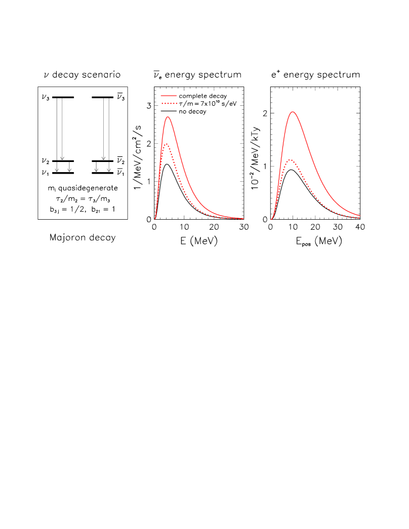
Figure 3: (Color online.) Supernova relic $\bar{\nu}_{e}$ spectrum (middle panel), and associated positron spectrum from $\bar{\nu}_{e}+p\to n+e^{+}$ (right panel), for a decay scenario with normal hierarchy and quasidegenerate masses (left panel, with $\tau/m$ and branching ratios assignments). The red and black solid curves correspond to the limiting cases of complete decay and no decay, respectively. The red dotted curves correspond to incomplete decay with $\tau/m=7\times 10^{10}$ s/eV. See the text for details.

For complete decay, the final state is populated by stable $\bar{\nu}_{1}$’s only, coming both from the initial $\bar{\nu}_{1}$ component ($Y_{\bar{\nu}_{1}}=Y_{\bar{\nu}_{e}}$) and from fully decayed $\bar{\nu}_{2,3}$’s ($Y_{\bar{\nu}_{2}}+Y_{\bar{\nu}_{3}}=2Y_{\nu_{x}}$, see Table I), with unaltered neutrino energies (QD case in Table II). The final relic $\bar{\nu}_{e}$ density (given by $\cos^{2}\theta_{12}$ times the final density of $\bar{\nu}_{1}$) is thus obtained by redshifting an initial yield equal to $\cos^{2}\theta_{12}Y_{\bar{\nu}_{e}}+2\cos^{2}\theta_{12}Y_{\nu_{x}}$. In the case of no decay for normal hierarchy, the initial yield is instead given by $\cos^{2}\theta_{12}\,Y_{\bar{\nu}_{e}}+\sin^{2}\theta_{12}Y_{\nu_{x}}$ [see Eq. (29)]. Therefore, while the $Y_{\bar{\nu}_{e}}$ component is the same in the two cases, the weight of the $Y_{\nu_{x}}$ component for complete decay is $2\cos^{2}\theta_{12}\simeq 1.42$, much larger than for no decay, where the weight is $\sin^{2}\theta_{12}\simeq 0.29$. The stronger weight of $Y_{\nu_{x}}$ for complete decay leads to the increase in normalization, peak energy, and width, which is visible in Fig. 3.

For incomplete neutrino decay (i.e., for $\tau/m\sim O(10^{10})$ s/eV), one expects an intermediate situation leading to a SRN flux moderately higher than for no decay. Figure 3 displays the results for a representative case ($\tau/m=7\times 10^{10}$ s/eV, red dotted curves), as obtained through the general solution of the kinetic equations worked out in Sec. III. Summarizing, the decay scenario examined in this section can lead to an increase of the SRN rate, as compared with the case of no decay. The enhancement can be as large as a factor $\sim 2$, the larger the more complete is the decay.

IV.3 Three-family decays for normal hierarchy and $m_{1}\simeq 0$

In this section we consider a representative decay scenario which provides observable SRN densities generally comparable to the no-decay case. The scenario assumes that the mass hierarchy is normal ($+\Delta m^{2}$) and that the lightest state is basically massless ($m_{1}\simeq 0$), so that $m_{2,3}\gg m_{1}$ and the approximation of strong hierarchy (SH) can be applied to the decays of $\nu_{2,3}$ (and of $\bar{\nu}_{2,3}$).

According to Table II (SH case), we can take $B(\nu_{2}\to\nu_{1})=B(\nu_{2}\to\bar{\nu}_{1})=1/2$. For the sake of simplicity, we extend such “branching ratio democracy” to all the $\nu_{3}$ decay channels, namely, we take $B(\nu_{3}\to\nu_{1})=B(\nu_{3}\to\bar{\nu}_{1})=B(\nu_{3}\to\nu_{2})=B(\nu_{3}\to\bar{\nu}_{2})=1/4$. We also assume $\tau_{3}/m_{3}=\tau_{2}/m_{2}\equiv\tau/m$, so that, as in the previous section, there is only one free parameter ($\tau/m$). The cases of no decay, incomplete decay, and complete decay, are then obtained for $\tau/m$ much larger, comparable, or much smaller than $O(10^{10})$ s/eV, respectively.

Figure 4 shows the supernova relic $\bar{\nu}_{e}$ and positron spectra for this scenario where, as depicted in the left panel, all decay channels are open. The results for the no-decay limit (solid curves) are identical to those in Fig. 3 and are not discussed again. The middle panel in Fig. 4 shows that the neutrino spectrum for complete decay (green solid curve) is significantly enhanced at low energy, as compared with the one for no decay. The positron spectrum, however, is very similar in the two cases (right panel). These features can be understood as follows.

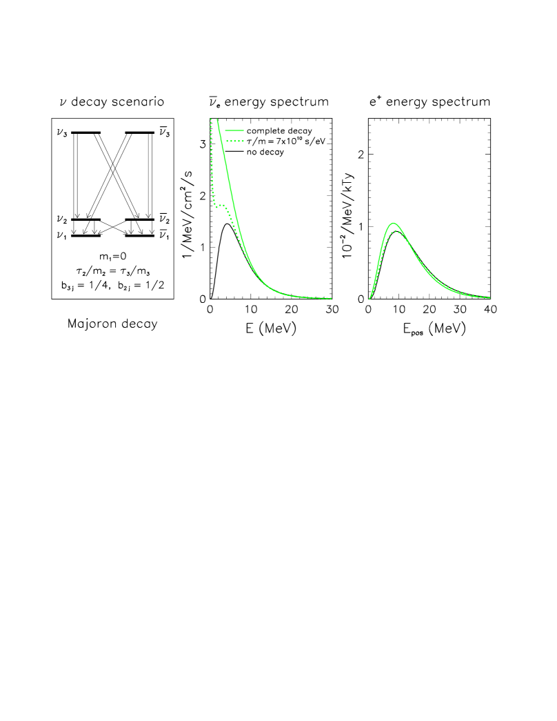
Figure 4: (Color online.) Supernova relic $\bar{\nu}_{e}$ spectrum (middle panel), and associated positron spectrum from $\bar{\nu}_{e}+p\to n+e^{+}$ (right panel), for a decay scenario with normal hierarchy and $m_{1}\simeq 0$ (left panel, with $\tau/m$ and branching ratios assignments). The green and black solid curves correspond to the limiting cases of complete decay and no decay, respectively. The green dotted curves correspond to incomplete decay with $\tau/m=7\times 10^{10}$ s/eV. See the text for details.

For complete decay, the final yield of stable $\bar{\nu}_{1}$’s comes both from the initial $\bar{\nu}_{1}$’s and from a complex decay chain, through the action of the operators $\cal D$ and $\overline{\cal D}$ [Eqs. (46) and (47)]:

$$\bar{\nu}_{1}\longrightarrow\bar{\nu}_{1} \Longrightarrow Y_{\bar{\nu}_{1}}\ ,$$ (48)

$$\bar{\nu}_{2}\stackrel{{\scriptstyle\frac{1}{2}\cal D}}{{\longrightarrow}}\bar{\nu}_{1} \Longrightarrow \frac{1}{2}{\cal D}Y_{\bar{\nu}_{2}}\ ,$$ (49)

$$\nu_{2}\stackrel{{\scriptstyle\frac{1}{2}\overline{\cal D}}}{{\longrightarrow}}\bar{\nu}_{1} \Longrightarrow \frac{1}{2}{\overline{\cal D}}Y_{\nu_{2}}\ ,$$ (50)

$$\bar{\nu}_{3}\stackrel{{\scriptstyle\frac{1}{4}\cal D}}{{\longrightarrow}}\bar{\nu}_{1} \Longrightarrow \frac{1}{4}{\cal D}Y_{\bar{\nu}_{3}}\ ,$$ (51)

$$\nu_{3}\stackrel{{\scriptstyle\frac{1}{4}\overline{\cal D}}}{{\longrightarrow}}\bar{\nu}_{1} \Longrightarrow \frac{1}{4}{\overline{\cal D}}Y_{\nu_{3}}\ ,$$ (52)

$$\bar{\nu}_{3}\stackrel{{\scriptstyle\frac{1}{4}\cal D}}{{\longrightarrow}}\bar{\nu}_{2}\stackrel{{\scriptstyle\frac{1}{2}\cal D}}{{\longrightarrow}}\bar{\nu}_{1} \Longrightarrow \frac{1}{8}{\cal D}\,{\cal D}Y_{\bar{\nu}_{3}}\ ,$$ (53)

$$\bar{\nu}_{3}\stackrel{{\scriptstyle\frac{1}{4}\overline{\cal D}}}{{\longrightarrow}}\nu_{2}\stackrel{{\scriptstyle\frac{1}{2}\overline{\cal D}}}{{\longrightarrow}}\bar{\nu}_{1} \Longrightarrow \frac{1}{8}{\overline{\cal D}}\,{\overline{\cal D}}Y_{\bar{\nu}_{3}}\ ,$$ (54)

$$\nu_{3}\stackrel{{\scriptstyle\frac{1}{4}\overline{\cal D}}}{{\longrightarrow}}\bar{\nu}_{2}\stackrel{{\scriptstyle\frac{1}{2}\cal D}}{{\longrightarrow}}\bar{\nu}_{1} \Longrightarrow \frac{1}{8}{\cal D}\,{\overline{\cal D}}Y_{\nu_{3}}\ ,$$ (55)

$$\nu_{3}\stackrel{{\scriptstyle\frac{1}{4}\cal D}}{{\longrightarrow}}\nu_{2}\stackrel{{\scriptstyle\frac{1}{2}\overline{\cal D}}}{{\longrightarrow}}\bar{\nu}_{1} \Longrightarrow \frac{1}{8}{\overline{\cal D}}\,{\cal D}Y_{\nu_{3}}\ .$$ (56)

This chain leads to a SRN density equation for complete decay formally similar to Eq. (29) (no decay), but with the integrand in square brackets replaced by $\cos^{2}\theta$ times the sum of the terms in Eqs. (48)–(56):

$$\cos^{2}\theta_{12}\left(Y_{\bar{\nu}_{1}}+\frac{1}{2}{\cal D}Y_{\bar{\nu}_{2}}+\dots+\frac{1}{8}{\overline{\cal D}}{\cal D}Y_{\nu_{3}}\right)\ .$$ (57)

In the above expression for complete decay, terms which are linear and quadratic in the convolution operators produce a substantial enhancement of the SRN energy spectrum at low energy, visible as a “pile-up” of decayed neutrinos with degraded energy in the middle panel of Fig. 4. At high energy, however, such terms happen to provide a contribution which is numerically close to the no-decay term $\sin^{2}\theta_{12}Y_{\nu_{x}}$ in Eq. (29), so that the high-energy tails of the SRN spectra for no decay and for complete decay (black and green solid curves in the middle panel of Fig. 4) are accidentally very similar to each other. Analogously, the case of incomplete decay (e.g., $\tau/m=7\times 10^{10}$ s/eV, green dotted curves), is appreciably different from the cases of no decay and of complete decay only at low energy.

In this scenario, the interesting effects of decay are almost completely confined to low $\bar{\nu}_{e}$ energies, and are thus washed out in the observable $e^{+}$ spectrum, due to the cross section enhancement of high-energy features. In fact, the $e^{+}$ spectra for the three cases of complete, incomplete, and no decay, turn out to be very similar to each other (right panel of Fig. 4).

In conclusion, from the results of this section we learn that there are neutrino decay scenarios which, despite a relatively complex structure (see Fig. 4), cannot be distinguished from the no decay case through future SRN observations, for any value of $\tau/m$ above the safe bound in Eq. (8). Similarly, such scenarios do not alter the “standard” (no-decay) SN 1987A phenomenology, and thus provide a particularly clean example of how the naive limit in Eq. (9) can actually be evaded.

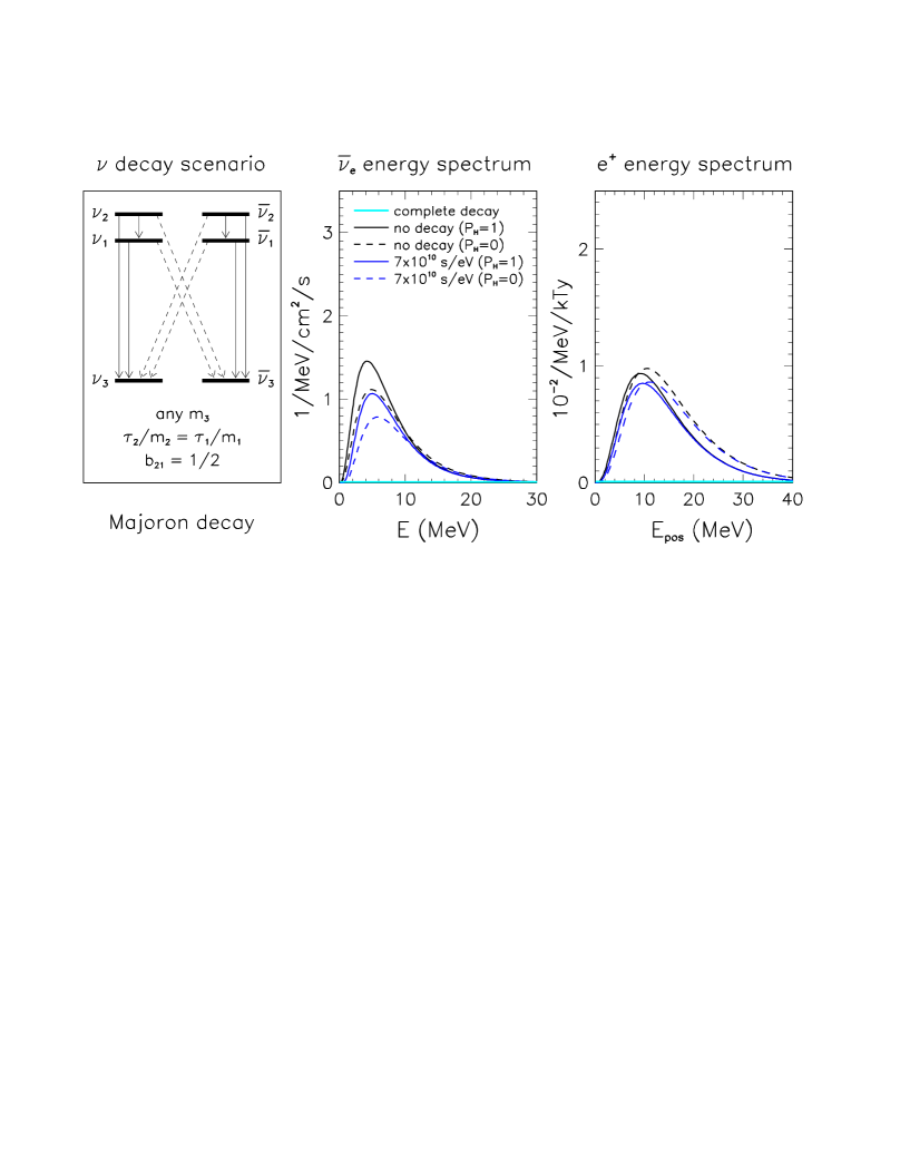
Figure 5: (Color online.) Supernova relic $\bar{\nu}_{e}$ spectrum (middle panel), and associated positron spectrum from $\bar{\nu}_{e}+p\to n+e^{+}$ (right panel), for a decay scenario with inverted hierarchy and generic $m_{3}$ (left panel, with $\tau/m$ and branching ratios assignments). The black and the blue curves correspond, respectively, to no decay and to incomplete decay with $\tau/m=7\times 10^{10}$ s/eV, for both $P_{H}=1$ (solid) and $P_{H}=0$ (dashed). The horizontal (light blue) line at $\sim 0$ corresponds to the case of complete decay. See the text for details.

IV.4 Three-family decay for inverted hierarchy

We conclude our survey of $3\nu$ decays by discussing a scenario where the SRN density is generally suppressed, as compared with the case of no decay. The scenario assumes an inverted mass hierarchy ($-\Delta m^{2}$), a fixed branching ratio $B(\bar{\nu}_{2}\to\bar{\nu}_{1})=1/2\ [=B(\nu_{2}\to\nu_{1})]$, and $\tau_{1}/m=\tau_{2}/m\equiv\tau/m$. Under these assumptions, only the decay $\bar{\nu}_{2}\to\bar{\nu}_{1}$ (where the QD approximation is applicable) is relevant to SRN observations. In fact, decays to $\bar{\nu}_{3}$ provide a negligible amount of $\bar{\nu}_{e}$’s ($\propto\sin^{2}\theta_{13}$). In particular, as graphically reported in the left panel of Fig. 5, the absolute value of $m_{3}$ makes no difference: It only opens (closes) the “dashed” decay channels for $m_{3}\simeq 0$ ($m_{3}$ large), with no change on the relic $\bar{\nu}_{e}$ flux for fixed $B(\bar{\nu}_{2}\to\bar{\nu}_{1})$. In the above scenario, the case of complete decay ($\tau/m\ll O(10^{10})$ s/eV) is trivial: since the final state is populated only by $\bar{\nu}_{3}$ (and $\nu_{3}$), the relic density of $\bar{\nu}_{e}$ is negligibly small ($\propto\sin^{2}\theta_{13}$).

The nontrivial case of incomplete decay ($\tau/m\sim O(10^{10})$ s/eV) is then expected to lead to an intermediate suppression of the SRN density. Figure 5 shows the numerical results for the specific value $\tau/m=7\times 10^{10}$ s/eV, in both cases $P_{H}=1$ (solid curves) and $P_{H}=0$ (dashed curves). The neutrino spectra for incomplete decay (blue curves) appear to be systematically lower than the corresponding no-decay spectra (black curves), although the difference is mitigated in the positron spectra (right panel of Fig. 5). A more substantial suppression of the positron spectrum can be obtained by lowering $\tau/m$ (see next subsection). In conclusion, in the inverted hierarchy scenario of Fig. 5, the SRN signal is generally suppressed by neutrino decay, and can eventually disappear for complete decay.

IV.5 Overview and summary of $3\nu$ decay

In the previous three subsections we have discussed, for three rather different scenarios, the cases of no decay [$(\tau/m\gg O(10^{10})$ s/eV], of complete decay [$\tau/m\ll O(10^{10})$ s/eV], and of incomplete decay for a specific value of $\tau/m$ ($=7\times 10^{10}$ s/eV). We think it useful to show also the behavior of the SRN signal for continuous values of the free parameter $\tau/m$.

Figure 6 shows the positron event rate integrated in the energy window $E_{e^{+}}\in[10,20]$ MeV which, although lower than the current SK window SKSN , might become accessible to future, low-background SRN searches GADZ . For each scenario, the rate is normalized to the standard expectations for no decay and normal hierarchy (NH), and is plotted as a function of $\tau/m$. The black solid line represents the reference case (no decay in NH), which is indistinguishable from the case of no decay with inverted hierarchy (IH) and $P_{H}=1$ (see Sec. II D). The black dashed line refers instead to the no-decay case with IH and $P_{H}=0$. For no decay, variations in the hierarchy or in $P_{H}$ appear to induce relatively small effect, which might be difficult to uncover once realistic experimental and theoretical uncertainties are considered in future SRN observations. Decay effects, however, enlarge dramatically the possible range of observable positron rates provided that $\tau/m$ is in the cosmologically interesting range below $O(10^{11})$ s/eV [See Eq. (10)]. For $\bar{\nu}$ decay in the quasidegenerate NH spectrum of Sec. IV B (red curve in Fig. 6), the positron rate rapidly increases for decreasing $\tau/m$, and reaches the “complete decay plateau” already at $\tau/m\sim O(10^{9})$ s/eV, with an asymptotic enhancement by a factor $\sim 2.3$. In the case of IH spectrum considered in Sec. IV D (solid and dashed blue curves in Fig. 6), conversely, the positron rate vanishes when approaching $\tau/m\sim O(10^{9})$ s/eV, for both cases $P_{H}=1$ (solid) and $P_{H}=0$ (dashed). Finally, for the NH spectrum with $m_{1}\simeq 0$ of Sec. IV C (green curve in Fig. 6), the positron rate appears to be almost the same as for no decay, at any value of $\tau/m$.

Summarizing, neutrino decay can enlarge the reference no-decay predictions for observable positron rates by any factor $f$ in the range $\sim[0,2.3]$.

Since the current experimental upper bound on the SRN flux from SK SKSN is just a factor of $\sim 2$–3 above typical no-decay expectations SKSN ; An03 (including those in this work), future observations below such bound are likely to have an impact on neutrino decay models. If experimental and theoretical uncertainties can be kept smaller than a factor of two (a nontrivial task), one should eventually be able to rule out, at least, either the lowermost or the uppermost values in the range $f\in[0,2.3]$, i.e., one of the extreme cases of “complete decay.” Optimistically, one might then try to constrain specific decay models and lifetime-to-mass ratios through observations (a goal not reachable with current information Ando ). Degeneracy between decay and no decay in specific models (as the one considered in Sec. IV C) will, however, set intrinsic limitations to SRN tests of neutrino lifetimes.

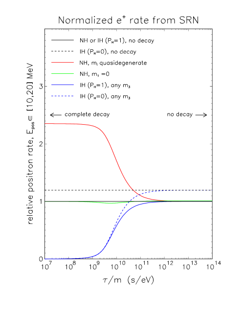
Figure 6: (Color online.) Positron event rates in the energy range $[10,20]$ MeV for various decay scenarios, normalized to standard expectations for normal hierarchy and no decay. The $\tau/m$ range in abscissa is well above the safe bound in Eq. (8). Notice how the expectations branch out (and then reach the complete decay limit) in the cosmologically relevant range $\tau/m\lesssim 10^{11}$ s/eV. See the text for details.

V Conclusions and PROSPECTS

Neutrino decays with cosmologically relevant neutrino lifetimes [$\tau_{i}/m_{i}\lesssim O(10^{11})$ s/eV] can, in principle, be probed through observations of supernova relic $\bar{\nu}_{e}$ (SRN). We have shown how to incorporate the effects of both flavor transitions and decays in the calculation of the SRN density, by finding the general solution of the neutrino kinetic equations for generic two-body nonradiative decays. (Radiative decays are briefly commented upon in Appendix A.) We have then applied such solution to three representative decay scenarios which lead to an observable SRN density larger, comparable, or smaller than for no decay. In the presence of decay, the expected range of the SRN rate is significantly enlarged (from zero up to the current upper bound). Future SRN observations can thus be expected to constrain at least some extreme decay scenarios and, in general, to test the likelihood of specific decay models, as compared with the no-decay case.

In this work we have focused on theoretical SRN calculations, and have not attempted a phenomenological analysis of the sensitivity to neutrino decay through prospective SRN experimental data, as those which might be collected, e.g., in the proposed Gd-doped Super-Kamiokande detector GADZ , in Hyper-Kamiokande Hype , or in the UNO project UNNO . Such analysis would require a detailed characterization of the many uncertainties affecting both the background-subtracted SRN signal and the theoretical inputs, especially those related to supernova simulations and to the star formation rate. These uncertainties, although currently rather large, are likely to decrease in the future as more powerful supernova codes and new astrophysical observations will become available (including, hopefully, a galactic supernova explosion). When significant improvements will be made in this direction, a systematic approach to SRN predictions and to their uncertainties will certainly be required, in order to interpret future SRN data and to use them to constrain nonradiative neutrino lifetimes in a range [up to $\tau/m\sim O(10^{11})$ s/eV] which is both largely unexplored and difficult to access by other means.

Appendix A Radiative decays of supernova relic neutrinos

Radiative neutrino decays El74 ; Pe77 of the kind

$${\stackrel{{\scriptstyle{}_{(-)}}}{{\nu}}\!\!}_{j}\to\ {\stackrel{{\scriptstyle{}_{(-)}}}{{\nu}}\!\!}_{i}+\gamma\$$ (58)

have been considered in a number of papers (see, e.g., Dolg ; Pakv ; PaVa ; Raft and references therein). Limits on the neutrino lifetime/mass ratio $\tau/m$ for such decay modes can be derived from a variety of arguments Raft . E.g., one of the strongest bounds,

$$\tau/m\gtrsim O(10^{20})\ \mathrm{s/eV}\ ,$$ (59)

is set by the nonobservation of infrared (IR) photons that would be emitted by Big Bang relic neutrinos Ress and, in addition, by the nonobservation of scattering of high energy [$O$(TeV)] photons from distant sources on this hypothetical IR background Bill . In the context of supernova neutrinos, the lack of excess $\gamma$ flux during the SN 1987A neutrino burst sets a limit $\tau/m\gtrsim O(10^{15})$ s/eV KoTu ; Raft . In this Appendix, we estimate phenomenological limits on $\tau/m$ from SRN radiative decays which, to our knowledge, have not been discussed so far in the literature.

Hypothetical radiative decays of SRN produce a diffuse photon background, whose local $(z=0)$ density per unit of volume and energy is obtained by integrating over the (redshifted) source terms $q^{\gamma}_{ji}$,

$$n_{\gamma}(E_{\gamma})=\int_{0}^{\infty}\frac{dz}{H(z)}\sum_{ji}^{m_{j}>m_{i}}q_{ji}^{\gamma}(E_{\gamma}(1+z),z)$$ (60)

where the $q^{\gamma}_{ji}$ have an expression analogous to Eq. (37), but with the appropriate final-state energy distribution for the photon in the laboratory frame,

$$\psi^{\gamma}_{\nu_{j}\to\nu_{i}}(E_{j},E_{\gamma})=\frac{m^{2}_{j}}{E_{j}\,\Delta m^{2}_{ji}}\left(1-\alpha+2\alpha\frac{E_{\gamma}\,m^{2}_{j}}{E_{j}\Delta m^{2}_{ji}}\right)\$$ (61)

(for $E_{j}>E_{\gamma}\Delta m^{2}_{ji}/m^{2}_{j}$), where $\Delta m^{2}_{ji}=m^{2}_{j}-m^{2}_{i}$, and the so-called asymmetry (or anisotropy) parameter $\alpha$ quantifies the amount of parity violation in the decay Raft ; Wilc ($\alpha\in[-1,+1]$ for Dirac neutrinos, while $\alpha=0$ for Majorana neutrinos Raft ). In calculating the photon density $n_{\gamma}$ from Eqs. (60) and (37), one can assume at first order that the neutrino density at any $z$ is basically “undecayed,” namely

$$n_{\nu_{j}}(E,z)\simeq n^{0}_{\nu_{j}}(E,z)=\frac{1}{1+z}\int_{0}^{\infty}\frac{dz^{\prime}}{H(z^{\prime})}R_{\mathrm{SN}}(z^{\prime})Y_{\nu_{j}}\left(E\frac{1+z^{\prime}}{1+z}\right)\ ,$$ (62)

as derived from Eq. (44) in the limit $\Gamma_{j}m_{j}/E_{j}\to 0$. This assumption will be validated a posteriori below.

In order to perform numerical calculations, the neutrino mass and decay parameters must be fixed. We assume a representative NH scenario with $m_{1}=0$, so that $m^{2}_{j}/\Delta m^{2}_{ji}\simeq 1$ (strong hierarchy approximation) and the $\psi$ function in Eq. (61) becomes the same for all decay channels. We also assume that $\tau_{2}/m_{2}=\tau_{1}/m_{1}\equiv\tau/m$, so that the total photon flux is

$$n_{\gamma}(E_{\gamma})=(\tau/m)^{-1}\int_{0}^{\infty}\frac{dz}{H(z)}\int_{E_{\gamma}}^{\infty}\frac{dE^{\prime}}{E^{\prime}}\psi(E^{\prime},E_{\gamma})\sum_{j=2,3}n^{0}_{\nu_{j}}(E^{\prime},z)\ ,$$ (63)

independently of the decay branching ratios (provided that they add up to unity, i.e., that only radiative decays occur). In the above equation, the inner sum extends to all the unstable states (both $\nu$ and $\bar{\nu}$). From Table I, it follows that the relevant neutrino yield to be integrated is

$$Y_{\nu_{2}}+Y_{\nu_{3}}+Y_{\bar{\nu}_{2}}+Y_{\bar{\nu}_{3}}=Y_{\nu_{e}}+3Y_{\nu_{x}}\ ,$$ (64)

for any value of $P_{H}$.

Figure 7 shows the results for the photon flux $n_{\gamma}(E_{\gamma})$ in the above scenario, assuming $\tau/m=10^{14}$ s/eV and three representative values $\alpha=-1,0,+1$, corresponding to green, red, and blue curves, respectively. The curves cross at $E_{\gamma}\simeq 1.21$ MeV, where the $\alpha$-dependent part of the integral in Eq. (63) vanishes. Lower (higher) values of $\tau/m$ would simply shift the curves upwards (downwards) along the $y$-axis. In the same figure, we superpose (as a dashed line) the best fit to the experimental $\gamma$ background flux measured by the COMPTEL experiment for $E_{\gamma}\in[0.1,\,30]$ MeV COMT ,

$$n_{\gamma}^{\mathrm{bkgd}}(E_{\gamma})\simeq 4\pi\times(1.05\pm 0.2)\times 10^{-4}\left(\frac{E_{\gamma}}{5\ \mathrm{MeV}}\right)^{-2.4}\mathrm{\ cm}^{-2}\mathrm{\ s}^{-1}\mathrm{\ MeV}^{-1}\ .$$ (65)

From Fig. 7 we derive that, in order to keep the $\gamma$ flux from hypothetical SRN decay below the observed $\gamma$ background, it must be

$$\tau/m\gtrsim O(10^{14})\mathrm{\ s/eV}\ ,$$ (66)

up to an $\alpha$-dependent factor of $O(1)$. Similar results would be obtained for inverted hierarchy and $m_{3}=0$ (not shown). Notice that this limit largely justifies a posteriori the “undecayed” approximation for $n_{\nu}$ in Eq. (62).

We do not further elaborate the SRN constraint in Eq. (62), since it is not competitive with the one in Eq. (59). We note, however, that the supernova relic neutrino bound in Eq. (66) is stronger than the one coming from the diffuse extragalactic stellar neutrino background [$\tau/m\gtrsim O(10^{12})$ s/eV] recently discussed in Fior .

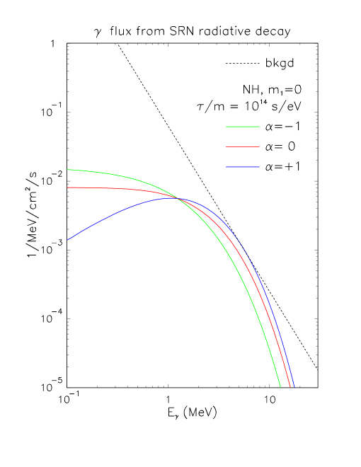
Figure 7: (Color online.) Energy spectrum of the photon flux coming from hypothetical radiative decays of SRN (solid curves), in a scenario with normal hierarchy, $m_{1}=0$, and $\tau_{2}/m_{2}=\tau_{3}/m_{3}=10^{14}$ s/eV. The calculations are performed for three representative values of the decay asymmetry parameter $\alpha$ ($=-1,0,+1$). The dashed line represents the power-law best fit to the $\gamma$ background measured by the COMPTEL experiment in the range $E_{\gamma}\in[0.1,30]$ MeV COMT .

Appendix B Remarks on $3\nu$ oscillations of the atmospheric neutrino background

In water-Cherenkov detectors, $3\nu$ flavor transitions affect not only the $e^{+}$ signal induced by supernova relic $\bar{\nu}_{e}$, but also the $e^{\pm}$ background induced by low-energy atmospheric neutrinos. The irreducible components of the $e^{\pm}$ background SKSN ; Male are due to (1) interactions of atmospheric $\nu_{e}$ and $\bar{\nu}_{e}$; and (2) decays of “invisible” $\mu^{\pm}$ (below the threshold for Cherenkov emission), induced by low-energy atmospheric $\nu_{\mu}$ and $\bar{\nu}_{\mu}$. In Super-Kamiokande SKSN , the background components (1) and (2) are characterized by parent neutrino energy spectra peaked at $E\sim 100$ and $E\sim 150$ MeV, respectively Male .

In SKSN , the effects of neutrinos oscillations on the $e^{\pm}$ background are calculated by assuming pure $2\nu$ oscillations in the $\nu_{\mu}\to\nu_{\tau}$ channel with maximal mixing (i.e., $\delta m^{2}\simeq 0$, $\theta_{13}\simeq 0$, and $\sin^{2}\theta_{23}\simeq 1/2$). Within the $2\nu$ approximation, the background component (1) is not affected by oscillations, while the component (2) is suppressed by the average effect of $\Delta m^{2}$-driven oscillations, through a factor $f_{\mu}=\sin^{2}2\theta_{23}\sin^{2}(1.27\Delta m^{2}L/E)\simeq 0.5\sin^{2}2\theta_{23}\simeq 0.5$, where $[\Delta m^{2}]=\mathrm{eV}^{2}$, $[L]=\mathrm{m}$, and $[E]=\mathrm{MeV}$. In terms of averaged flavor oscillation probabilities $P_{\alpha\beta}$, the $2\nu$ approximation implies that $(P_{ee},P_{\mu\mu},P_{\mu e})\simeq(1,\,0.5,\,0)$ SKSN .

We remark, however, that the $2\nu$ approximation $\delta m^{2}\simeq 0$, usually valid for typical atmospheric neutrino energies ($\gtrsim 1$ GeV), is not applicable in the SRN context. Indeed, for $E\sim O(100)$ MeV and $L\sim O(R_{\oplus})$, the associated oscillation phase cannot be neglected [$\delta m^{2}L/E\sim O(1)$]. Even for $\theta_{13}=0$, the low-energy atmospheric neutrino background is thus sensitive to the “solar” $\delta m^{2}$, rather than to the “atmospheric” $\Delta m^{2}$ (which can be effectively taken as $\infty$).

The possibility of probing $\delta m^{2}$-driven oscillations at very low atmospheric $\nu$ energy ($\ll 1$ GeV) would deserve, in itself, a separate investigation. Here we only make some rough estimates of the relevant flavor oscillation probabilities $P_{\alpha\beta}$ for $\delta m^{2}\neq 0$. We assume isotropic atmospheric neutrino fluxes (produced at $h=20$ km from the ground level), equal components of $\nu$ and $\bar{\nu}$ (with weights 3 and 1, respectively, to account for the different cross sections), and a $\nu_{\mu}/\nu_{e}$ flavor ratio $r=2$. Matter effects are estimated through a constant-density approximation for the Earth. The oscillations parameters are taken from Eqs. (3)–(6), with either $\sin^{2}\theta_{13}=0$ or $\sin^{2}\theta_{13}=0.067$ [see Eq. (7)]. We consider a representative neutrino energy $E=100$ MeV, and average over all incoming $\nu$ directions.

Under these assumptions, and for $\sin^{2}\theta_{13}=0$, we find $(P_{ee},P_{\mu\mu},P_{\mu e})\simeq(0.77,\,0.42,\,0.11)$, which differ significantly from the values $(1,\,0.5,\,0)$ obtained by setting $\delta m^{2}=0$. The atmospheric electron events [background (1)] and invisible muon events [background (2)] are then modulated, respectively, by the factors $f_{e}\simeq P_{ee}+rP_{\mu e}\simeq 0.99$ and $f_{\mu}\simeq P_{\mu\mu}+P_{ee}/r\simeq 0.48$, which happen to differ only slightly from the values $(f_{e},\,f_{\mu})=(1,\,0.5)$ considered in SKSN by setting $\delta m^{2}=0$. Analogously, for $\sin^{2}\theta_{13}=0.067$ we find $(P_{ee},P_{\mu\mu},P_{\mu e})\simeq(0.67,\,0.17,\,0.41)$ and $(f_{e},\,f_{\mu})\simeq(1.01,\,0.50)$. Therefore, despite significant $\delta m^{2}$-induced effects on the oscillation probabilities, the irreducible atmospheric background rates do not appear to be significantly modified as compared with those obtained by (incorrectly) setting $\delta m^{2}=0$, independently of the value of $\sin^{2}\theta_{13}$.

In conclusion, the approximation $\delta m^{2}=0$ is not applicable, in principle, to the analysis of the irreducible atmospheric neutrino background in SRN searches SKSN . However, in practice, this approximation does not appear to be harmful (according to our provisional estimates). More refined estimates of $\delta m^{2}$-driven oscillations might be of some interest in future high-statistics SRN searches UNNO ; Hype , which are expected to find a signal above the irreducible atmospheric $\nu$ background. These oscillation effects would instead loose interest if the “irreducible” background could be “reduced away” by tagging SRN events, as recently proposed in GADZ .

References

- (1) V. Barger, D. Marfatia and K. Whisnant, Int. J. Mod. Phys. E 12, 569 (2003); M. C. Gonzalez-Garcia and Y. Nir, Rev. Mod. Phys. 75, 345 (2003); C. Giunti and M. Laveder, hep-ph/0310238; G. Altarelli and K. Winter (editors), Neutrino Mass, Springer Tracts in Modern Physics 190 (2003).
- (2) K. Hagiwara et al. [Particle Data Group Collaboration], Phys. Rev. D 66, 010001 (2002).
- (3) G.L. Fogli, E. Lisi, A. Marrone, and A. Palazzo, hep-ph/0309100, to appear in Phys. Lett. B.
- (4) G.L. Fogli, E. Lisi, A. Marrone, D. Montanino, A. Palazzo, and A.M. Rotunno, Phys. Rev. D 69, 017301 (2004).
- (5) A.D. Dolgov, Phys. Rept. 370, 333 (2002).
- (6) S. Pakvasa, hep-ph/0305317, in the Proceedings of the 10th International Workshop on Neutrino Telescopes (Venice, Italy, 2003), edited by M. Baldo-Ceolin (U. of Padua Publication, Italy, 2003), p. 469.
- (7) G. Gelmini and E. Roulet, Rept. Prog. Phys. 58, 1207 (1995).
- (8) S. Pakvasa, hep-ph/9905426, in the Proceedings of the 8th International Workshop on Neutrino Telescopes (Venice, Italy, 1999), edited by M. Baldo-Ceolin (U. of Padua Publication, Italy, 1999), p. 283.
- (9) J.F. Beacom and N.F. Bell, Phys. Rev. D 65, 113009 (2002); see also A. Bandyopadhyay, S. Choubey, and S. Goswami, Phys. Lett. B 555, 33 (2003).
- (10) KamLAND Collaboration, K. Eguchi et al., hep-ex/0310047.
- (11) J.A. Frieman, H.E. Haber, and K. Freese, Phys. Lett. B 200, 115 (1988).
- (12) J.F. Beacom, N.F. Bell, D. Hooper, S. Pakvasa, and T.J. Weiler, Phys. Rev. Lett. 90, 181301 (2003); G. Barenboim and C. Quigg, Phys. Rev. D 67, 073024 (2003).
- (13) Super-Kamiokande Collaboration, M. Malek et al., Phys. Rev. Lett. 90, 061101 (2003).
- (14) M.S. Malek, PhD thesis (SUNY, Stony Brook, 2003), available at www-sk.icrr.u-tokyo.ac.jp/sk/pub/index.html .
- (15) S. Ando, Phys. Lett. B 570, 11 (2003).
- (16) J.F. Beacom and M.R. Vagins, hep-ph/0309300, submitted to Phys. Rev. Lett.
- (17) C.K. Jung, hep-ex/0005046. See also the site: superk.physics.sunysb.edu/nngroup/uno .
- (18) K. Nakamura, Int. J. Mod. Phys. A 18, 4053 (2003).
- (19) S. Ando, K. Sato, and T. Totani, Astropart. Phys. 18, 307 (2003).
- (20) S. Ando and K. Sato, Phys. Lett. B 559, 113 (2003).
- (21) M. Fukugita and M. Kawasaki, Mon. Not. Roy. Astron. Soc. 340, L7 (2003).
- (22) L.E. Strigari, M. Kaplinghat, G. Steigman, and T.P. Walker, astro-ph/0312346.
- (23) S. Ando, astro-ph/0401531.
- (24) P. Madau et al., Mon. Not. Roy. Astron. Soc. 283, 1388 (1996); P. Madau, M. Della Valle, and N. Panagia, Mon. Not. Roy. Astron. Soc. 297, 17 (1998).
- (25) See, e.g., SDSS Collaboration, M. Tegmark et al., astro-ph/0310723.
- (26) G.L. Fogli, E. Lisi, D. Montanino, and A. Palazzo, Phys. Rev. D 65, 073008 (2002) [Erratum-ibid. D 66, 039901 (2002)].
- (27) L. Wolfenstein, Phys. Rev. D 17, 2369 (1978); S.P. Mikheev and A.Yu. Smirnov, Yad. Fiz. 42, 1441 (1985) [Sov. J. Nucl. Phys. 42, 913 (1985)].
- (28) R.C. Schirato and G.M. Fuller, astro-ph/0205390; G.L. Fogli, E. Lisi, D. Montanino, and A. Mirizzi, Phys. Rev. D 68, 033005 (2003).
- (29) T.K. Kuo and J. Pantaleone, Rev. Mod. Phys. 61, 937 (1989).
- (30) C. Lunardini and A.Yu. Smirnov, JCAP 0306, 009 (2003).
- (31) G.G. Raffelt, M.T. Keil, R. Buras, H.T. Janka, and M. Rampp, astro-ph/0303226, to appear in the Proceedings of NOON 2003, 4th International Workshop on Neutrino Oscillations and their Origin (Kanazawa, Japan, 2003); M.T. Keil, G.G. Raffelt, and H.T. Janka, Astrophys. J. 590, 971 (2003).
- (32) P. Vogel, Prog. Part. Nucl. Phys. 48, 29 (2002); P. Vogel and J. F. Beacom, Phys. Rev. D 60, 053003 (1999).
- (33) M. Lindner, T. Ohlsson and W. Winter, Nucl. Phys. B 607, 326 (2001).
- (34) Z.G. Berezhiani and M.I. Vysotsky, Phys. Lett. B 199, 281 (1987); Z.G. Berezhiani, G. Fiorentini, M. Moretti, and A. Rossi, Z. Phys. C 54, 581 (1992).
- (35) C. Giunti, C. W. Kim, U.W. Lee, and W.P. Lam, Phys. Rev. D 45, 1557 (1992).
- (36) M. Kachelriess, R. Tomàs, and J.W.F. Valle, Phys. Rev. D 62, 023004 (2000).
- (37) Z.G. Berezhiani and A.Yu. Smirnov, Phys. Lett. B 220, 279 (1989).
- (38) K. Choi and A. Santamaria, Phys. Rev. D 42, 293 (1990).
- (39) R. Tomàs, H. Päs, and J.W.F. Valle, Phys. Rev. D 64, 095005 (2001).
- (40) Y. Farzan, Phys. Rev. D 67, 073015 (2003).
- (41) E.W. Kolb and M.S. Turner, The Early Universe (Westview Press, Boulder, 1994).
- (42) Y. Chikashige, R. Mohapatra, and R. Peccei, Phys. Lett. B 98, 265 (1981); G. Gelmini and M. Roncadelli, Phys. Lett. B 99, 411 (1981).
- (43) S. Pakvasa and J.W.F. Valle, hep-ph/0301061.
- (44) G.G. Raffelt, Stars as Laboratories for Fundamental Physics (U. of Chicago Press, Chicago, 1996).
- (45) C.W. Kim and W.P. Lam, Mod. Phys. Lett. A 5, 297 (1990).
- (46) S. Eliezer and D.A. Ross, Phys. Rev. D 10, 3088 (1974).
- (47) S.T. Petcov, Sov. J. Nucl. Phys. 25, 340 (1977).
- (48) M.T. Ressel and M.S. Turner, Comments on Astrophys. 14, 323 (1990).
- (49) S.D. Biller et al., Phys. Rev. Lett. 80, 2992 (1998); see also the comment by G.G. Raffelt, Phys. Rev. Lett. 81, 4020 (1998).
- (50) E.W. Kolb and M.S. Turner, Phys. Rev. Lett. 62, 509 (1989).
- (51) L.F. Li and F. Wilczek, Phys. Rev. D 25, 143 (1982).
- (52) COMPTEL Collaboration, AIP Conf. Proc. 510, 392 (2000); S.C. Kappadath, PhD thesis (U. of New Hampshire, 1998), available at wwwgro.unh.edu/users/ckappada .
- (53) C. Porciani, S. Pietroni, and G. Fiorentini, astro-ph/0311489.
- (54) O.L.G. Peres and A.Yu. Smirnov, hep-ph/0309312.